Examination of different wall jet and impinging jet concepts to produce large-scale downburst outflow

Introduction

Thunderstorm downburst winds are stochastic, non-stationary, non-Gaussian, localized, highly turbulent, and extreme weather phenomena that produce high intensity winds. Downbursts descend as a powerful jet of cold downdraft wind as a result of atmospheric convection, impinge vertically downwards into the ground, and diverge a ring vortex that curls up and include an outflow in all radial directions (Fujita, 1985, 1990). This outflow has the form of a 3-D radial wall jet, creating severe horizontal wind velocities that lead to substantial damage to surrounding structures. Downbursts are characterized by their strong, highly spatiotemporal variable wind shear stresses near the ground (Zhu and Etkin, 1985), which impose a significant threat to low, medium, and high buildings and long span structures such as transmission lines and suspension bridges. The horizontal maximum wind velocities, which typically exceed conventional design wind speeds, can reach up to 75 m/s (Letchford et al., 2002), occurring at heights between 30 and 100 m above the ground (Holmes, 1999; Hjelmfelt, 2002; Lin & Savory, 2006) and with relatively short durations lasting from 2 to 30 min (Selvam and Holmes, 1992; Letchford et al., 2002; Lin and Savory, 2006). The sizes of downbursts can be classified as microbursts ($\le$ 4 km diameter) and macrobursts ($>$ 4 km diameter), where microbursts are the most detrimental. Extreme wind events in the form of tornadoes and downbursts constitute 70% of the worldwide natural disasters (Solari, 2016). Recent reports (Hoogewind et al., 2017; NOAA, 2018; Dunsavage, 2020) indicate an increasing number of strong convective thunderstorms, which accounts for billions of dollars in infrastructure damage and more than 150 fatalities on a yearly basis in the United States and worldwide. Exacerbating future extreme windstorm risks are indications from climate science that more intense downbursts should be expected (Hoogewind et al., 2017). Also, downbursts are the most common cause of severe winds with a higher occurrence than tornadoes (Aboshosha, 2014). Apart from causing various aircraft accidents, forest destruction, and loss of life, downbursts are the main cause of damage for many buildings every year due to strong winds and high suction pressures affecting the building facades, causing destruction on cladding elements, flying of projectile debris, and thousands of roof blow-offs (Abd-Elaal et al., 2018). Nevertheless, transmission power lines and towers are the type of structures that suffer the most (Solari, 2018), with several hundred failures, collapses that leave behind a trail of economic devastation. However, limited research has been focused on understanding the interaction between extreme downburst winds and structures. The current lack of knowledge pertaining to downburst flow characterization and their impacts on the built environment has motivated researchers to simulate large downburst outflows in a laboratory set-up to assess downburst wind effects on the built environment. However, the physical simulation of large-scale downburst outflows implicates a great challenge due to the high complexity level of the 3-D outflow and their unique spatial and temporal localized nature. Fujita, 1986 was the first to use an impinging jet (IJ) mechanism in a laboratory setting by using an inverted plastic cylinder aloft blowing air vertically downward into a circular plate with holes emanating smoke and visualizing the formation and development of the ring vortex. Since then, several researchers have continued to simulate downbursts using a variety of solutions including numerical and experimental methods. Numerical methods include 1) analytical IJ (Oseguera and Bowles, 1988; Selvam and Holmes, 1992; Kim and Hangan, 2007), 2) analytical vortex ring (Zhu and Etkin, 1985; Ivan, 1986; Vicroy, 1992), 3) empirical (Holmes & Oliver, 2000; Li et al., 2012), 4) hybrid models (Chen and Letchford, 2004; Solari et al., 2017), 5) Monte Carlo techniques (Wang et al., 2013; Huang, 2015; Peng et al., 2017), and 6) CFD simulations (Proctor, 1988, 1989; M. S. Mason et al., 2009a; Vermeire et al., 2011; Zhang et al., 2013a, 2013b; Aboshosha et al., 2015). Experimental methods are classified into three categories such as 7) the fluid release method by buoyancy-driven fluid or cooling source (Lundgren et al., 1992; Alahyari and Longmire, 1994), 8) the impinging jet (IJ) (Letchford and Chay, 2002; Mason et al., 2007; McConville et al., 2009; Richter et al., 2018; Junayed et al., 2019), and 9) the wall jet using strategic modifiers in the classic wind tunnel to achieve the redirection of flow. The fluid release method, also known as the cooling source or ring vortex, depends on submerging one denser fluid into another less dense fluid and obtaining negative driving buoyancy that represents the atmospheric convection, in which a cold air impinges through the hot air found near the ground level. Although this method is the best representation of a downburst phenomenon in its entirety (i.e., from formation to dissipation), it is not applicable to structural testing applications because of their small outflow scales generated with Reynolds numbers (Re) in the order of ${10}^3$ (Mason et al., 2007; Mason et al., 2009a; Lin et al., 2015) and less than $\text{Re}=\mathrm{70,000}$, which represents a threshold value needed for a proper downburst outflow to develop (Mason et al., 2007; Lin et al., 2015). The second method is the impinging jet (IJ), which was utilized for downburst applications by Fujita (1985), Holmes (1992), Wood et al. (2001), Chay and Letchford (2002), Letchford and Chay (2002), Mason et al. (2005), and McConville et al. (2009). The IJ is an axisymmetric, circular turbulent forced jet of air obtained from a nozzle with diameter D impinging into a wall orthogonally at a distance H and spreading out radially a turbulent 3-D wall jet as seen in Figure 1A. The impinging jet (IJ) has three flow regions that assimilate the formation, evolution, and development of a full-scale downburst. The outflow or 3-D radial wall jet region exhibits a growth of the wall jet thickness $\delta$ at a distance downstream from the center of the stagnation region, also known as a touchdown. It includes the maximum radial velocity of a downburst ${\overline{U}}_{\max }\left(x,y,z,t\right)$ at a peak height $z_{\max }$, which constitute two main parameters of importance for structural applications. Sengupta and Sarkar, 2008 suggested that the IJ is the best representation of a full-scale real downburst making this test reliable for structural engineering applications. However, assumptions exist in the way the IJ is implemented. For example, a typical IJ produces a single, axisymmetric jet of air mostly at a stationary position. However, downbursts dynamics are complex as they involve the formation of clustered and unsymmetrical geometries (not necessarily circular), translating during the downdraft impingement and hitting the ground at a tilt (Mason et al., 2009b). For this reason, the IJ method is limited and can only be classified in three categories to account for these particular dynamic complexities as follows: 1) the IJ type that includes stationary and steady impinging jets (Letchford and Illidge, 1999; Wood et al., 2001; Hangan et al., 2004; Sarkar et al., 2006; Sengupta and Sarkar, 2008; Xu and Hangan, 2008; Zhang et al., 2013a; Jesson et al., 2015; Elawady et al., 2017), which entails opening the nozzle and leaving it open, hence allowing the jet flow run continuously and hitting a wall orthogonally, 2) the second IJ type includes stationary and transient (pulsed) jets (Landreth and Adrian, 1990; Hangan et al., 2004; McConville et al., 2009; Jesson et al., 2015; Jubayer et al., 2016), which entails using a valve control mechanism that allows a pulse of air exit the nozzle momentarily; the term “pulse” meaning a short-lived, isolated downdraft of air, and 3) the third IJ type includes a translating nozzle with a steady jet (Letchford et al., 2002; Mason et al., 2005; Hangan et al., 2017; Asano et al., 2019), which entails a continuous flow of air hitting an orthogonal wall while moving the nozzle sideways during this operation. An example of this test is found at the WindEEE facility that has a diameter range between 1.6 and 4.5 m and can simulate IJ while translating at a wind velocity of 2 m/s over a horizontal distance of 5 m (Hangan et al., 2017).

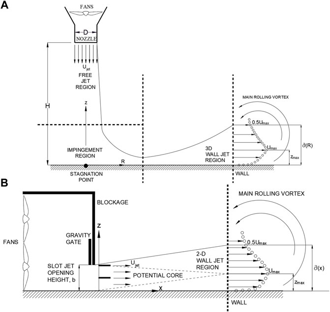
FIGURE 1. (A) Impingement jet model, credit: Sengupta and Sarkar, 2008. (B) 2-D Wall jet test model, credit: Lin and Savory, 2006; 2012.

The typical procedure for the IJ is to maintain a fixed height to diameter ratio H/D, where H is the distance from the nozzle tip to the orthogonal wall surface, and D is the nozzle diameter that represents the jet diameter of the flow before impingement into the orthogonal wall surface. The recommended value for H/D was found to be larger than one, in order to be able to develop a complete main ring vortex (Kim et al., 2007) so that a significant large 3-D outflow size with a maximum horizontal velocity is obtained downstream from the stagnation point. The outflow is dependent upon the lower values of Re but start to become independent at $\text{Re}=\mathrm{70,000}$ (Mason et al., 2007; Mason et al., 2009a; Lin et al., 2015). It is always recommended to maximize the Re in laboratory simulations as much as possible to mitigate possible scaling effects (Lin and Savory, 2006; Xu and Hangan, 2008). The 2-D plane wall jet application has shown great feasibility to create larger outflows than any other existing downburst simulation methods as shown in Figure 1B. The typical 2-D plane wall jet method can be achieved by using different means for redirecting the flow near the ground surface in a classic wind tunnel. The 2-D wall jet provides a simpler and more compact outflow to prevent lateral expansion as is the case of the 3-D radial wall jet flows from an IJ application (Van Hooff et al., 2012). A 2-D wall jet is defined as a shear flow along a wall that is produced by an inertial supplied momentum from a slot opening where the stream-wise velocity over some region within the shear flow exceeds that of the external stream (Launder and Rodi, 1983). The 2-D wall jet consists of an inner layer and outer layer. The inner layer (i.e., boundary layer) constitutes a highly turbulent viscous layer that starts from the wall to the height of maximum velocity $z_{\max }$ and it contains the characteristics of the conventional ABL properties. The outer layer extends from above $z_{\max }$ to the outer edge of the flow and consists of a free shear layer, also known as the mixing region. The strong interaction of these two layers at the interface form a complex turbulent outflow that is difficult to characterize. It is relevant to note that the wall jet thickness $\partial$ constitutes both layers up to where the velocity is reduced to that value above the shear layer. It is usually calculated up to the height where half of the maximum local velocity is reached. Several examples of previous 2-D wall jets used in downburst applications include the addition and/or modification at the lower part of a classic wind tunnel by introducing a slot jet near the wall region (Lin and Savory, 2006; Lin et al., 2007). Other 2-D wall jet examples include the operational control of strategic individual fans from a multi-fan assembly generating a gust front near the wall (Cao et al., 2002; Sassa et al., 2009; Zhao et al., 2009), the addition of rotating plates (Matsumoto, 1984) or shutters (Matsumoto, 2007), and the addition of blades connected to a stepper motor and rotated at different angles of incidence (Butler and Kareem, 2007; Aboutabikh et al., 2019; Le and Caracoglia, 2019). The advantage of the 2-D wall jet method over the IJ is that it enables the creation of larger sized outflows in smaller spaces. However, the Reynolds numbers achieved in the majority of the 2-D wall jet tests presented in Table 1 (except for the large-scale 2-D wall jet at the University of Western Ontario) have low values compared to the Reynolds number achieved by the largest IJ facility at WindEEE. The reason is because these previously tested 2-D wall jets have been implemented in small scales only. It is important to note that the 2-D wall jet simulation method is limited as it is does not enable the simulation of the downburst formation, free jet or impingement but only considers the outflow region that occurs after downdraft impingement (O’Donovan, 2005). This is particularly crucial for structural testing applications with the opportunity of reducing a Re dependency. The 2-D wall jet has a higher potential to achieve larger Reynolds numbers than the IJ method in a smaller space because it depends on fewer geometrical variables. For example, the 2-D wall jet depends on the height of the slot opening b, the jet velocity $U_{jet}$, and the surface roughness length $z_0$, whereas the IJ not only depends on these geometrical variables mentioned but also on the ratio H/D, where H is the height from the ground to the tip of the nozzle and D is the diameter of the nozzle. Thus, for IJ applications, a large space is required to maintain a reasonable H/D $\ge$ 1 and simulate proper 3-D outflows away from the center of impingement. In the case of the 2-D wall jet, a smaller space for testing can be utilized as demonstrated by Abdelwahab et al. (2022) for the design of a multi-purpose wind tunnel that allows the development of ABL, tornadoes, and 2-D downburst outflows in a reduced space. Other advantages of the 2-D wall jet are that it offers a more economical solution, ease of assembly, and simpler testing. On the other hand, the drawbacks of the 2-D wall jet include the limited size of the wind tunnel, possible boundary condition effects from the side walls, and roof or any other solid obstacles in the testing area, which could disturb the size and quality of the produced downburst outflow. Also, the 2-D wall jet discards relevant properties of the downbursts that the IJ include such as a strong viscous-inviscid interaction between a primary and secondary layer at impingement that can further increase $z_{\max }$ to higher elevations (Walker et al., 1987; Mason et al., 2010). Another example is the translating or tilt effect happening in real downbursts, which can only be carried out in the IJ. At the end, the 2-D wall jet outflow is just a representation of a “vertical slice” of the 3-D outflow field as obtained in a real full-scale downburst and IJ test set-up (Le and Caracoglia, 2020). The 2-D wall jet is very limited in only producing a single primary rolling vortex of significant size exiting the slot height b. Table 1 shows the various Reynolds number (Re) that represent the typical outflow sizes that can be attributed to various downburst real full-scale events, experimental IJ and 2-D wall jets. Several criteria have been previously adopted to estimate the Reynolds number in downburst applications as follow: for real downburst events are based on $z_{\max }$ (Fujita, 1981; Hjelmfelt, 1988), IJ tests are based on the nozzle diameter D (Junayed et al., 2019), and 2-D wall jet tests based on $z_{\max }$ (Lin et al., 2015) or the slot height b (Lin and Savory, 2006, 2010). The corresponding values of these experimental Re values will give an approximate outflow size despite the different parameters used to calculate Re. There must be a consistency in the calculation method used when comparing the Re of full-scale downburst events to the Re from experiments by using the same parameters. The most practical parameters to use would be the peak velocity ${\overline{U}}_{\max }$ and peak height $z_{\max }$ as presented in Table 1.

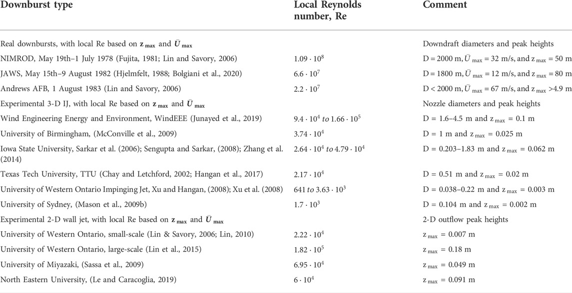
TABLE 1. Typical Reynolds numbers of full-scale and experimental downbursts.

IJ tests are widely used among wind engineers because these tests provide a closer approximation to real downbursts. It is noted from Table 1 that the largest IJ is the WindEEE facility with a Re value three orders of magnitude smaller than the average Re value from a real downburst like the NIMROD full-scale event. The smaller Re values of experimental tests demonstrate a mismatch of the kinematic similarities between full-scale and experimentally simulated downburst events. The main motivation of the current article is to simulate and characterize a reliable downburst outflow of significant size at the National Science Foundation (NSF)-designated Experimental Facility (EF) Wall of Wind (WOW) to further extend the current capabilities of the national facility. The study aims to identify and optimize the design concept of a large-scale downburst simulator that is suitable for structural aerodynamic and aeroelastic testing at larger scales. Also, to investigate how the peak height $z_{\max }$ is affected by the topography and increase of the surface roughness length $z_0$. This article outlines the development and comparison of results among five different downburst simulator designs: one of a 2-D IJ type and four 2-D wall jet types. One downburst simulator will be chosen and tested in a smooth terrain and two different roughnesses to determine the quality of the outflow and the turbulent statistical characteristics of the downburst outflow. The results are compared to published results from previous field measurements, numerical analysis, and experimental results.

Experimental set-up

Wall of Wind Experimental Facility

The NSF-Natural Hazard Engineering Research Infrastructure (NHERI) Wall of Wind (WOW) Experimental Facility (EF) located in Miami, Florida is a large-scale, conventional, and boundary layer open jet wind testing facility that is capable of testing small- to full-scale destructive and non-destructive models of various types of civil engineering structures. It consists of an arched plenum, contraction section, and a flow management box that allows an open jet flow to be discharged downstream into a testing section area. An airflow of 135.9 m³/s is achieved by using twelve propeller fans arranged in two rows by six columns arc pattern with an individual fan diameter of 1.83 m and operated by respective fan motors that deliver a total power of 6,264 kW altogether. The range of wind velocities are initialized from a minimum of 4.47 m/s to a maximum of 71.53 m/s, hence reaching Saffir–Simpson category five hurricane wind velocities. It also includes a set of vertical spires that help produce ABL characteristics in the exiting flow and consists of a mechanically operated roughness elements that allows the modification of various surface roughness conditions. Figure 2A shows the intake and Figure 2Bshows the exit of the WOW facility. The produced ABL wind flow field is equal to the size of the flow management box cross-sectional area of 6.1 m wide by 4.3 m high and passes through a 4.9 m diameter turntable center (where the test models are fixed at the base) located at 6 m from the flow management box outlet. The overall longitudinal fetch of the wind flow field exiting the flow management box outlet and passing through the turntable section is a total of 11.63 m long. More details on design, dimensions, and construction of the full-scale WOW can be found in the following articles by Chowdhury et al. (2017), Chowdhury et al. (2018). Strategic downstream horizontal locations away from the wind jet initiation (i.e., flow management outlet) are analyzed in this study including the turntable front (TTF), turntable center (TTC), and turntable back (TTB).

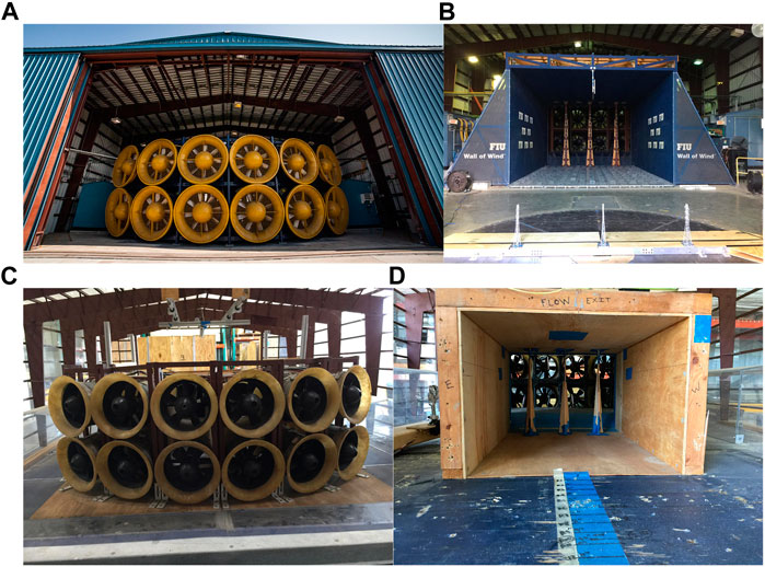
FIGURE 2. (A) Full-scale WOW intake; (B) full-scale WOW flow management box; (C) small-scale 1:15 WOW intake; and (D) small-scale 1:15 WOW flow management box.

Small-scale Wall of Wind

The WOW EF is equipped with a 1:15 replica of the flow simulator (called small-scale WOW thereafter), which contains identical components of the full-scale WOW flow management box including the spires, the arched plenum, and testing section. The small-scale WOW serves to carry out physical testing for new preliminary designs and concepts to assess the wind flow behavior before implementation at higher cost at the full-scale facility. The small-scale WOW is built out of wood and is run by a system of twelve electronic operating propeller fans of 127 mm diameter each. A piece of control software runs the twelve fans velocity and operation duration. The current study involves the tryouts of five different downburst simulators in the small-scale WOW so that one of these can be selected and be built in the large-scale WOW. In addition to a smooth plywood surface in the testing section floor of the small-scale WOW (assumed to be open terrain in this study), two different roughness with varying thicknesses were added to the test section floor to account for the effect of increasing surface roughness length $z_0$ on downburst flow fields. Figures 2C,D show the intake and exit of the small-scale WOW, respectively, as similarly presented in Figures 2A,B for the full-scale WOW. The dimensions of flow management box of small-scale WOW are 397 mm wide by 291 mm high and provide a characteristic ABL profile. A maximum wind velocity of 12 m/s at a height of 178 mm was measured with an anemometer when running all twelve fans at 10% of the rpm throttle capacity of the system, which was used for all downburst tests in this study.

Downburst simulator designs

As mentioned earlier, five different downburst simulator options were designed and tested in the small-scale WOW. One 2-D IJ simulator and four 2-D wall jet simulators were considered and tested in the small-scale WOW to simulate downburst flows. Figure 3 shows schematics of all five downburst simulator options. For Option A, as seen in Figure 3A, a blockage is installed in front of the flow management box, completely shutting the WOW flow field and redirecting the wind upward. The compartment with controllable louvers stores a volume of air of 1,282 cm³. When a downburst is desired, the venting louvers will be closed, and a second set of louvers will open, allowing wind to flow downward on the turntable side of the blockage wall, creating a 2-D impinging jet that collides with the ground and forms a downburst-like vortex. Controlling the duration of time for opening/closing the louvers would allow for control of the downburst event duration. After the IJ takes place, a single main rolling vortex is formed traveling across the testing section downstream. The three regions conforming the IJ, the free jet, the impingement and outflow region are maintained with this type of downburst simulator. This type of simulator is one of a kind as it enables converting a classic wind tunnel into a 2-D IJ like downburst simulator without the need of blowers and nozzles positioned vertically and oriented downward. Option B, shown in Figure 3B, consisted of an opening near the ground and a fixed set of venting louvers placed at an angle of ${45}^{\circ }$ upward, which were used to reduce the built-up wind and avoid any possible back flow pressure hindering the WOW fans while in operation. In this design, the downburst ramp-up and ramp-down wind speed time history behavior was obtained using a gravity gate (GG) placed between the flow management box exit and the downburst simulator. The GG was completely blocking the opening, then pulled up quickly so that it momentarily allowed the wind flow exit near the bottom region for a short period of time and then closed back by free fall so that it returned to the original position behind the slot opening. The use of the GG as a mechanism for opening and closing was abrupt. Option C in Figure 3C consisted of four louver slats, while both Option D in Figure 3D and Option E in Figure 3E consisted of two louver slats. The reduction in the number of the louver slats was to enable more simplicity in the construction and operation phases. For both options, D and E, the louver slats were placed at the lower region of the downburst simulator and were set to open and close in an automated rotational mechanism. This close–open–close actuator mechanism was operated by means of servo motors rotating the slat’s supporting rods about their cross-sectional axes. The louver slats were closed (i.e., placed in a vertical position) and opened while rotating gradually counterclockwise ${70}^{\circ }$ and staying at ${20}^{\circ }$ angle with reference to horizontal position. In Option E, Figure 3E has the same opening configuration and lower slat of Option D but with a different closing mechanism, consisting of a gravity gate (GG) that drops down to block the flow based on a preset time duration determined based on the desired downburst target duration. The experimental protocol used herein on all downburst simulator options included taking flow measurements of 26 horizontal downstream distances away from the 2-D wall jet initiation in increments of 25.4 mm, and mainly concentrating on three strategic positions within the testing section area indicated by the turntable front (TTF), turntable center (TTC), and turntable back (TTB) in order to study the wind flow field evolution and wall jet growth. For all downburst simulators herein, each test run lasted 20 s, and longitudinal wind velocity measurements were obtained at different heights. The opening and closing time for all downburst simulator systems were programmed to last 3 s. The opening started at the 8 s marker and closed at the 11 s marker.

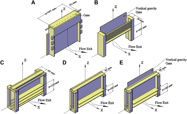
FIGURE 3. Downburst simulator options: (A) Option A, (B) Option B, (C) Option C, (D) Option D, and (E) Option (E)

Addition of roughness

The floor of the testing section consists of a plywood surface, representing a smooth terrain condition. In addition, two surface roughness of thickness 6 and 10 mm with a plastic and artificial grass texture were implemented to determine the variation in the outflow under the influence of surface roughness length $z_0$.

A schematic summary layout of the downburst simulator design process and selection is shown in Figure 4 to facilitate the work presented herein.

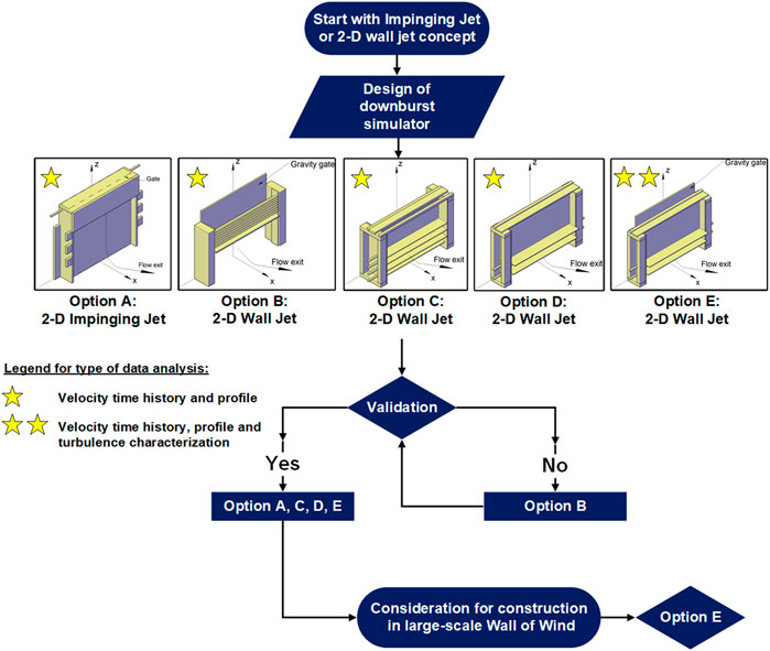
FIGURE 4. Schematic summary layout of the downburst simulation design process and selection.

Instrumentation and test plan

Two types of measurement probes were utilized to measure the wind velocities at different heights and horizontal distances in the test section. The two data acquisition systems consisted of a Scanivalve™ DSA 3217 with a sampling frequency of 500 Hz and a Turbulent Flow Instrumentation™ Series 100 Cobra probes with a sampling frequency of 2,500 Hz were used as shown in Figure 5A. The use of two different acquisition systems served as a validity cross-check between these two when repeated test runs were performed. Both acquisition systems complemented each other by providing an overall analysis of the downburst outflow development at strategic locations of the turntable as shown in Figure 5B. The Scanivalve™ DSA 3217 differential pressure measurements were obtained with sixteen pitot tubes made from brass hollow pipes of 0.36 mm internal diameter and were positioned in a vertical rake spaced at uniform height increments of 12.7 mm above the floor level reaching to a maximum height of 203.2 mm. The differential pressure or the dynamic wind pressure was obtained using the following Eq. 1:

where $\Delta p$ is the differential pressure, $p_{total}$ is the total pressure measured inside the pitot tube, $p_{static}$ is the static pressure, ${\rho }_{air}$ is the air density, and $U$ is the upstream longitudinal wind velocity. To check the test repeatability and as a cross-check, the Cobra probe’s rake was also placed at the same downstream horizontal distances coinciding with the Scanivalve™ pitot tube’s rake but this time considering different heights (because of the size difference), corresponding to z = 12.7, 50.8, 101.6, 152.4, and 203.2 mm, respectively.

FIGURE 5. (A) Side view of test section with measurement rakes. (B) Plan view of test section.

Discussion of results

Decomposition of downburst wind velocities

Downburst winds are non-stationary and localized in time with a sudden intense 2-D wall jet constituting a primary ring vortex growth. Downburst instantaneous total wind velocities are typically decomposed by a classical moving average filter into their moving mean and fluctuating wind velocities as suggested by Choi and Hidayat (2002), Chen and Letchford (2004), and Holmes et al. (2008), Solari et al. (2015). The total instantaneous wind velocity of a downburst at any height $z$ at any time $t$ and a downstream horizontal distance $x$ is defined as the vector summation of a central moving average wind velocity and a fluctuating wind velocity as follows:

where $U\left(x,y,z,t\right)$ is the total instantaneous wind velocity at height $z$ and time $t$; $\overline{U}\left(x,y,z,t\right)$ is the slowly varying, non-turbulent, and moving mean wind velocity, which is obtained from averaging the data using a convenient average time window $T_{ave}$; and $u^{\prime }\left(x,y,z,t\right)$ is the turbulent fluctuating wind velocity. The extraction of the slowly varying mean $\overline{U}\left(x,y,z,t\right)$ can also be carried out by different filtering methods other than the classical moving average such as the wavelet transform, Hilbert transform, and the empirical decomposition (Wang et al., 2013, 2014; Huang et al., 2015). The arbitrary selection of a suitable average time window $T_{ave}$ depends on a best visual fit. The filtering of the random fluctuations from the entire time domain should allow the moving mean wind velocity retain the changes found in the peak zone consisting of a ramp-up, plateau, and ramp-down (Lin and Savory, 2010). For any velocity time history decomposition of downburst winds, it can be noted that the residual fluctuating wind velocities also maintain a non-stationary pattern because of its transient, sharp, and sudden peak zone associated with the passage of a single rolling vortex. In order to analyze downbursts similarly to synoptic winds with a Gaussian behavior, a reduced turbulence fluctuation with a zero mean and unit standard deviation method was implemented by Solari et al. (2015) and shown in the following Eq. 3.

where $\stackrel{\sim }{u^{\prime }}$ is the reduced turbulence wind velocity; $u^{\prime }$ is the residual turbulence wind velocity, and ${\sigma }_{u^{\prime }}$ is the standard deviation of the residual turbulence wind velocity. A representative feature of downburst time history is the peak zone that demonstrates a sudden wind velocity rise composed of a ramp-up, plateau, and ramp-down. The sudden increase in the wind velocity is a result of the transient passage of a main rolling vortex which grows, decays, and eventually dissipates causing high turbulence. In this study, the instantaneous wind velocity time histories are decomposed into their slowly varying mean wind velocities $\overline{U}$ and residual fluctuating turbulent wind velocities $u^{\prime }$ using the classical moving average filter explained herein based on the ideal selection of a short and suitable average time $T_{ave}$ moving window (Holmes et al., 2008; Solari et al., 2015). Thus, arbitrary values of $T_{ave}$ were selected. The value $T_{ave}$ of 0.5 s was selected for simulator options C and D, while a smaller value $T_{ave}$ of 0.1 s was selected for simulator options A, B, and E, following the classical moving mean decomposition criteria. Figure 6 shows the moving mean horizontal velocity time histories for each of the five tested downburst simulators at the TTC in smooth terrain (i.e., Options A, B, C, D, and E in colored markers). The figure also shows the superposition of each of the tested simulations at the ramp-up and ramp-down to a measured downburst event moving mean velocity time history (black solid line) that occurred in port La Spezia, Italy (Solari et al., 2012; Romanic et al., 2020). This procedure was performed as a validation to a field downburst event and a check of performance for each downburst simulator. From this figure, the shape of the spike or “peak zone” is established for each downburst simulator.

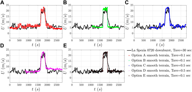
FIGURE 6. Velocity time history comparison among all downburst simulations for options a, b, c, d, e and a real downburst event Termed La Spezia 0720; courtesy of Professor Giovanni Solari and “Wind and Ports” and “Wind, Ports, and Sea” Campaigns.

In an attempt to validate whether the downburst main characteristics are obtained in the experimental simulations, the wind velocity time histories were scaled to match a full-scale downburst in time and velocity using Eqs 4, 5, respectively. The experimental results were superimposed to match the baseline and peak height mid-points of a real full-scale downburst, which is one of many recorded through the “Wind and Ports” (Solari et al., 2012) and “Wind, Ports, and Sea” (Repetto et al., 2018) ongoing campaign projects that have captured downburst outflows with high resolution anemometers.

where $U_{m,scaled}\left(t\right)$ and $T_{m,scaled}\left(t\right)$ are the scaled experimental velocity and time history of the small-scale downburst simulator, respectively; $U_m\left(t\right)$ and $T_m\left(t\right)$ are the actual velocity and time history obtained using the small-scale downburst simulators; and $B_m$ and $B_p$ are the corresponding horizontal baselines of the simulated and full-scale downburst flow, respectively. The baseline is drawn as a horizontal line by taking a mean wind velocity of the stationary process prior to the start of the ramp-up zone. A velocity scale ${\lambda }_U$ is defined as the ratio between the relative height from the baseline to the maximum velocity value of the small-scale downburst simulators (models) and the full-scale downburst (prototype). A time scale ${\lambda }_t$ is defined as the ratio between peak zone time duration of the experimental simulations and the peak zone time duration of the full-scale downburst. The peak zone time duration is defined herein as the difference between the time instant of the ramp-down mid-point minus the time instant of the ramp-up mid-point. Figure 6 shows that the shape of the time histories is not identical among the five different simulators. In some simulators the peak zone has a rectangular shape and others a triangular shape. The rectangular shape indicates a sudden, sharp, and abrupt change of wind velocities. This rectangular unique trend was found only in downburst simulator options B, D, and E from which B and E included the GG. The triangular peak zone shapes were found for the remaining downburst simulators A and C. In addition, as a second method to compare with field measurements, the slopes of the ramp-up and ramp-down, which represent the acceleration or deceleration respectively, were calculated. For example, the ramp-up acceleration values for the full-scale La Spezia 0720, option A, option B, option C, option D, and option E are 0.19, 0.18, 1.26, 0.16, 0.12, and 0.47 m/s², respectively. The ramp-down deceleration values are −0.11, −0.13, −0.87, −0.18, −0.11, and −0.92 m/s² for the same corresponding downbursts. All downburst exhibits a reasonable value for the accelerations that compares well with the acceleration value of the full-scale event. Option D is being on the low acceleration side, and Option B is on the high acceleration side. The use of a GG greatly increases the acceleration and deceleration happening in the ramp-up and ramp-down, respectively, in the case of Option B. This is because of the abrupt way the GG operates in the opening or closing mechanism. The opening of the slats in option E was shown to open much quicker than compared to option D despite being similar opening methods. This is due to a mechanical activation glitch found in the servo motors that open the louver slats at a faster rotational speed if the automation profile is set to open only and is slower for opening and closing mode. The rate of opening is fundamental in determining the ramp-up acceleration. Based on this result, in the author’s opinion, all the downburst simulator options tested herein are suited for the generation of typical downburst horizontal time histories. However, looking at the ramp-up and ramp-down zones, Option B should be excluded and considered failed.

Velocity profiles

The vertical velocity profile of the horizontal velocities with a typical “nose shape” is one of the primary downburst characteristics that differ significantly from the common atmospheric boundary layer (ABL) profile. Figure 7 shows the vertical profiles of the normalized moving mean horizontal velocities for all five tested simulators. Figure 7A shows the instantaneous velocity profiles measured at the time instant of the local maximum velocity at the TTC, and Figure 7B shows the envelope velocity profiles, which are defined as the local maximum velocities recorded across all times for each height. It can be seen from both figures that the shape of the nose is observed, with option A providing the largest peak height $z_{\max }$. It can also be seen that option E provides a steeper slope above the peak height than the rest of the options. The next steeper slope is exhibited by option B. Both options use a gravity gate, which confirms that the use of a gravity gate steepens the slope. Figure 7C shows the envelope of downburst vertical velocity profile for Option E at several downstream strategic locations of interest such as location of maximum velocity, TTF, TTC, and TTB. As in the case of Option E, it was noticed that all downburst simulators exhibit the global maximum velocity across the entire flow field ${\overline{U}}_{\max ,global}$ happening in the close vicinity of the louver slats opening. It can be seen that the slope of the vertical velocity profile becomes steeper as the outflow moves downstream. The figure also shows the velocity profile with the characteristic nose shape being preserved across the turntable at a further distance from the downburst simulator where scale models will be placed and tested at the WOW EF against downburst winds. Furthermore, from Figure 7D, it can be observed that the addition of roughness, representing an increase in the terrain surface roughness length $z_0$ at a distance downstream of the simulator, caused an increase of the peak height $z_{\max }$. This behavior is observed with smooth terrain obtaining a peak height of 12.7 mm, a surface roughness length of 6 mm resulting in a peak height of 25.4 mm, and a 10 mm surface roughness length resulting in a peak height of 50.8 mm. Figure 7E shows a comparison of the envelope normalized horizontal velocity profiles for all downburst simulators recorded at the TTC and compared with various other field, numerical, and experimental downburst measurements reported in the literature. All downburst simulator options provide a typical characteristic nose profile and prove that these downbursts simulator designs are readily applicable for conventional wind tunnel modification. It can also be seen from Figure 7E that Option A outflow tapers off sharper with height compared to the rest of the downburst simulator options. Option E profile from the pitot tube measurements provides a vertical velocity profile, resembling a nose shape outside of the shaded upper limit similarly to the study by Aboshosha et al. (2015).

FIGURE 7. Vertical velocity profiles of normalized horizontal wind velocities for: (A) instantaneous wind velocities at TTC; (B) envelope wind velocities at TTC; (C) envelope of Option E at different horizontal distances; (D) envelope of Option D and Option E at TTC for different roughness; and (E) horizontal velocity profile validation.

It is always recommended to maximize the simulated Re so that the flow becomes independent of the nozzle and jet initiation conditions and that the outflow simulation represents a proper downburst with a considerable surface friction and a wall jet thickness $\partial$ so that it can engulf large-scale models and minimize any scaling effects. As mentioned earlier, examples of Re for field and previously simulated downbursts are provided in Table 1. For the downburst simulator options A, B, C, D, and E tested herein, the local Reynolds numbers were calculated similarly in order to compare to previous Reynolds number from full-scale and previous downburst experiments. The results are presented in Table 2.

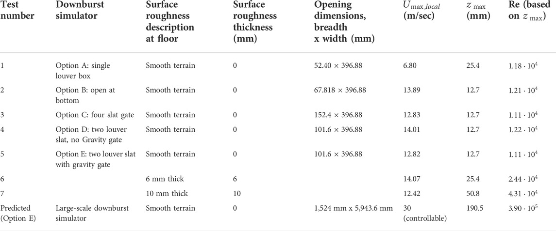
TABLE 2. Small-scale downburst test configurations at the WOW TTC.

From Table 2, it can be seen that Option A provides the higher peak height in smooth terrain over the other downburst simulator options. The range of Re obtained in the downburst simulators discussed herein vary between the smallest $R_e=1.11\cdot {10}^4$ from Option E to the largest $R_e=1.22\cdot {10}^4$ from Option D, using the pitot tubes in smooth terrain. Comparing this Re value range to the Re value range presented in Table 1 for those 2-D wall jet methods by previous researchers, the range presented herein for the tested simulators exceed the Re range values of previously reported studies. Since the small-scale WOW is 1:15 times smaller than the full-scale WOW EF, it can be predicted that the peak height $z_{\max }$ may reach as high as ∼190.5 mm, using the Reynold’s number formula described earlier, a predicted Reynold’s number of up to $3.90\cdot {10}^5$ can be obtained in the WOW EF, assuming a maximum wind speed of 30 m/s. Based on the adequate formation of a main rolling vortex observed from smoke visualization, simulation of the vertical profile of horizontal velocities resembling a “nose shape,” a peak zone or spike found within the velocity time history, and the large Re values obtained, in addition to practicality, constructability, and ease of operation, the downburst simulator Option E is the chosen simulator to be constructed in full-scale at the WOW. Thus, the focus of the remaining results discussion for the next sections will be on Options E and D. Figure 8 shows the time history for Option E at the TTC in smooth terrain for all 16 heights using the Scanivalve data acquisition system. A noticeable downburst peak zone of the wind velocity occurs at the lowest pitot tube height of 12.7 mm and as soon as the heights are increased, the downburst peak zone starts to diminish and disappears at a height of about 102 mm, which coincidentally is about the same value of the slot opening height of b = 102 mm. It was confirmed through smoke visualization that the main rolling vortex height passing through the TTC corresponds to those heights at which the downburst peak zone is still visible. At higher heights beyond 102 mm, the downburst peak zone has disappeared, but a turbulence perturbation is still visible within the peak zone.

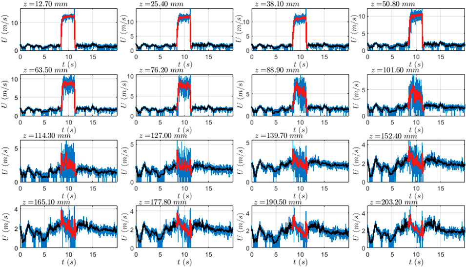
FIGURE 8. Downburst time history recorded at various heights using the 16 pitot tubes at the TTC using downburst simulator Option E in smooth terrain.

Figure 9A shows the temporal evolution of the instantaneous vertical velocity profile of the normalized mean horizontal wind velocities at TTC for downburst simulator Option E. Figure 9B shows the smoke visualization of the main rolling vortex provided by Option E. The passage of the main rolling vortex is marked by the presence of the nose shaped vertical velocity profile at specific time instants. At 10 s, the nose shape profile is observed. By 12 s, the downburst flow has already vanished at the TTC, and the wind velocities are back to almost zero as the gravity gate (GG) has shut down the flow.

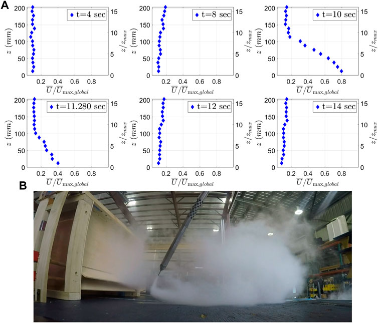
FIGURE 9. (A) Downburst evolution of the instantaneous vertical velocity profile of the mean horizontal wind velocities at TTC for simulator Option E. (B) Smoke flow visualization of main rolling vortex for Option E.

Figure 10 shows a snapshot of the growth of the wall jet thickness $\partial$, which is equal to the height at which the maximum velocity is half, $z_{0.5\cdot U_{\max }}$ (Knowles and Myszko, 1998; Mason et al., 2007; Mason et al., 2009a). The wall jet thickness is the result of the friction caused by the wall surface roughness on the flow that slides parallel to the wall surface. In smooth terrains, the wall jet thickness is very thin and tends to become quasi-inviscid or almost turbulent free. However, when the roughness length $z_0$ is large, the wall jet thickness is also large. This is what leads to the increase of the peak height $z_{\max }$ when the surface roughness $z_0$ is increased. The instantaneous time considered herein is the time at which the global peak velocity is occurring. It can be seen that the wall jet thickness measured at the location of the global maximum velocity, $x_{\max }$, is 46 mm and then starts to increase linearly as stipulated in the literature by Verhoff (1963). According to Mason et al. (2009b), the increase in the wall jet thickness leads to mean velocity gradients $\partial U/\partial z$ decrease, which is clearly observed here. There is an evident growth of the wall jet downstream of the downburst as well as retardation in each local maximum velocity downstream. The location of the global peak velocity was always in the near vicinity of the opening for all downburst simulators, despite trying out different downburst simulator designs with varying distances extending further away from the flow management box. The global peak velocity and horizontal distance downstream from the jet initiation were for option E, ${\overline{U}}_{\max ,global}=15.2m/s$, and $x_{\max }=152.4mm$.

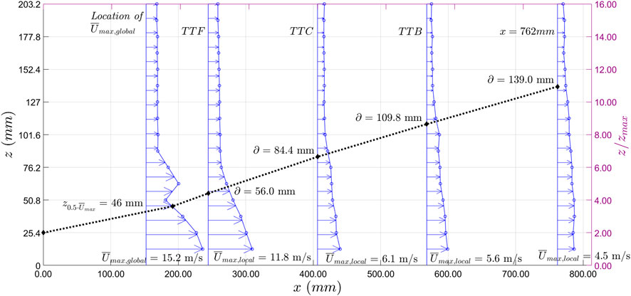
FIGURE 10. Downburst wall jet growth at the time of global peak velocity at various downstream distances for Option E.

Turbulence intensity

Turbulence, by definition, is the state of flow in which the inertial motion of turbulent eddies makes a dominant role in energy and momentum transfer (Makita, 1991). A great difficulty exists in obtaining these statistical quantities in downburst applications due to their non-stationary and transient properties. Thus, in the case of downbursts, it is difficult to quantify a turbulent flow structure in the same manner as it has been performed before for stationary processes such as atmospheric boundary layer (ABL) winds. The analysis herein evaluates the turbulence intensity, $I_{u^{\prime },T}$, quantities for downburst simulations for Option E to define the corresponding turbulence characterization. The turbulence intensity of non-stationary winds, as in the case of downbursts, can be defined as follows in Eq. 6:

where $E\left[\cdot \right]$ is the expected value within a short time interval $T$; ${\sigma }_{u^{\prime },T}$ is the standard deviation of the residual fluctuating wind velocity $u^{\prime }$ within a time interval $T$, and ${\overline{U}}_{\max ,T}\left(t\right)$ is the local maximum time varying mean wind velocity across all heights at the particular downstream horizontal of interest. A vertical profile of the longitudinal turbulence intensity indicates a measure of the strong fluctuating wind velocity deviations, occurring at different heights within the outflow. Figure 11 shows the turbulence intensity profile for downburst simulators D and E. The turbulence intensity increases with height for both system measurements. A similar trend was noticed from the literature by Jubayer et al. (2016), Le and Caracoglia (2019), and Aboutabikh et al. (2019) for different experimental simulations. The test measurements take into consideration smooth terrain for Option D and E as well as the addition of a 10 mm thick surface roughness for Option E. From these average measurements, it can be seen that the turbulence intensity values are higher for the thicker roughness, thus confirming that the increase of surface roughness increases the turbulence near the ground. For Option E, the measurements in the smooth terrain, $I_{u^{\prime },T}$, varies from 0.14 in the measurement near the ground up to a value of 0.17 at a higher height. For the 10 mm roughness, $I_{u^{\prime },T}$ varies from 0.20 in the measurement near the ground, then is reduced to 0.18 and increased again up to a value of 0.30 at higher heights. An average turbulence intensity value of 0.10 was reported by Aboshosha et al. (2015) in an open terrain using large-Eddy simulation (LES) models. In the case of Aboutabikh et al., 2019, the turbulence intensity values vary from 0.11 near the ground to a maximum value of 0.13 at a higher height. The values closer to the ground from the studies of Aboshosha et al. (2015), Aboutabikh et al. (2019), and Le and Caracoglia (2019) are smaller than the turbulence intensity values near the ground presented herein on smooth terrain. On the other hand, Jubayer et al., 2016 showed higher values.

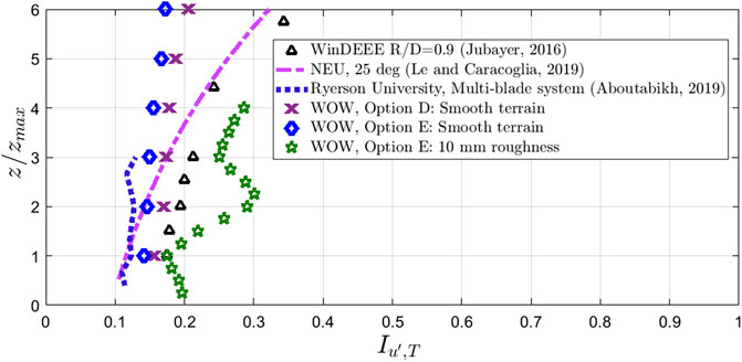
FIGURE 11. Turbulence intensity vertical profiles for downburst simulator Options D and E at the TTC for smooth terrain and 10-mm thick surface roughness.

The trend of the turbulence intensity profiles of Option D and Option E in Figure 11 agrees well with previous results from Jubayer et al., 2016 at the WindEEE dome IJ simulation, the multi-blade small-scale testing with louver slats tilted at 25° angle by Le and Caracoglia (2019) at North Eastern University (NEU) and the multi-blade 2-D wall jet by Aboutabikh et al. (2019). The magnitude of these values is related to the denominator selected in Eq. 6. Some authors like Wang and Kareem, 2004 and McCullough et al., 2014 select the denominator to be a mean of the moving mean value of the velocity and other authors like Elawady et al., 2017 prefer to select the maximum value of the moving mean velocity. This is one subjective decision of many that exist in the case of downbursts analysis. Another example is the selection of an adequate duration T. Several researchers select the start time of the downburst event before the ramp-up starts and sometime after the ramp-down to be the duration T. Others select the duration T to be at the start of the ramp-up and end of the ramp-down. The statistical characteristics within the peak duration of the event change significantly and differ from a stationary process. A ramp-up, a plateau zone, and a ramp-down contain their own duration and specific statistical characteristic. Thus, for downburst analysis, considering a combination of different statistical characteristics in one whole process is somewhat controversial. Usually the common trend for turbulence intensity profiles, both for synoptic and non-synoptic winds, tend to decrease as the height increases (Chay, 2001; Lombardo et al., 2018). In the case of downburst events in urban Beijing analyzed by Zhang et al. (2019), it can be observed that the turbulence intensity profiles have a variable “zigzag” trend with height, especially near the ground. This is not the case in the 2-D wall jet cases tested herein or the ones presented in the literature by Jubayer et al. (2016) or Le and Caracoglia (2019), where turbulence intensity increases with height. This situation may be due to the fact that these are tested in a limited space with side walls affecting the results from forming boundary layers. Also, the turbulent intensity values started to be measured at a height $z_{\max }$.This means that only the outer free shear layer of the 2-D wall jet is being considered and the inner ABL layer is being excluded. It is important to note that the fluctuation velocity $u^{\prime }$ and the slowly varying mean wind velocity ${\overline{U}}_T\left(t\right)$ are very high near the ground. However, as the height increases up to the center of the main rolling vortex, the moving mean velocity starts to reduce until it becomes almost zero, but the turbulence fluctuations are gradually reduced; hence, allowing the turbulence intensity to spike-up to the height at the center point of the rolling vortex as the denominator in Eq. 6 tends to zero. At further heights above the main rolling vortex center, the turbulence intensity then starts to decrease as the fluctuating velocities also decrease gradually. This unique trend is associated to a single main rolling vortex growing in size as it travels downstream across the testing section area. It is important to note that surrounding obstructions, side walls, and roof found in the testing area can also affect the quality of the 2-D outflow. The advantage of a large-scale wind tunnel facility with a 2-D wall jet application is that it allows a large main rolling vortex to pass through the testing section without boundary conditions formed by any side walls or roof in the near vicinity of the test section area with the possibility to measure the turbulence intensity at heights beneath $z_{\max }$. Measuring the turbulence intensity at lower heights than $z_{\max }$ is where the interest lies as these are the critical turbulence intensities affecting the low-rise buildings and transmission power line towers.

Power spectral density

Turbulence fluctuations can be visualized as the superposition of eddies or gusts of different sizes and frequencies. The integral length scale is an estimate of the average size of those eddies in the flow constituting turbulence. The difference between ABL and downburst turbulence characteristics is that the horizontal integral length scales are typically smaller in the case of downbursts because of their smaller scales, localized nature, and proximity to the ground (Solari et al., 2015). Three methods are commonly used by researchers in wind engineering to determine the integral length scales (Teunissen, 1980). These are the direct integration method, the exponential fit method and the power spectra fit method. Usually, the first and second methods derive the integral length scales from correlation functions. The third method can be used in two ways: first by applying a fast Fourier transform (FFT) in the residual fluctuation components $u^{\prime }$ as performed by Aboutabikh et al. (2019), which follows the same methodology for ABL stationary winds. The second way is by applying the FFT in the reduced fluctuation components $\stackrel{\sim }{u^{\prime }}$ as recommended by Solari et al. (2015) and followed by Le and Caracoglia (2019). Some of the available power spectral density (PSD) models in the literature that can be used for the residual and reduced turbulence fluctuations are presented in Table 3.

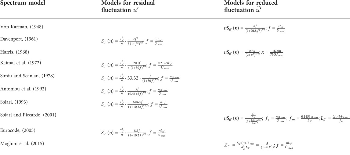
TABLE 3. Available power spectral density models in literature.

The preferred method for providing best results of the integral length scale among all methods presented for stationary systems is the exponential fit. In the case of downburst, given the difference in statistical quantities found in the ramp-up, plateau, and ramp-down, these methods may require modifications so that they can be utilized adequately. A common modification was discussed by Solari et al. (2015), where the PSD of a reduced fluctuation $\stackrel{\sim }{u^{\prime }}$ is taken into consideration so that the process is converted from a non-stationary to an equivalent stationary and that the conventional tools can be applied. In this case, both, application of the conventional PSD on residual fluctuations used for stationary process (Figure 12A) and application of PSD on reduced fluctuations for non-stationary process (Figure 12B) have been used. The PSD as well as the longitudinal integral length values were calculated for Option E at $z_{\max }$ at the TTC. From the PSD on residual fluctuations, the longitudinal integral length scale obtained for Option E was $L_{u^{\prime }}^x=0.087m$ by Von Karman PSD fit from Figure 12A and from exponential fit was $L_{u^{\prime }}^x=0.018m$. From Figure 12B, the longitudinal integral length scales obtained for Option E based on the PSD on the reduced fluctuations were $L_{\stackrel{\sim }{u^{\prime }}}^x=0.057m$ by Von Karman PSD fit and $L_{\stackrel{\sim }{u^{\prime }}}^x=0.059m$ by Solari and Piccardo PSD fit. The value from exponential fit on the reduced fluctuations was $L_{\stackrel{\sim }{u^{\prime }}}^x=0.022m.$ It can be seen that the integral length scale values obtained from the PSD on the reduced fluctuations were larger than the value obtained from the exponential fit. Also, the integral length scale values obtained from the PSD of the reduced fluctuations were smaller than the integral length scale value obtained from the PSD values on residual fluctuations. Solari et al., 2015 reported that for the La Spezia 0720 downburst event, the $L_{\stackrel{\sim }{u^{\prime }}}^x$ ranges from 27.5 to 32.7 m. From Figure 12B, the PSD fit between Option E and La Spezia 0720 event match very well in the low and high end of the turbulence spectrum. The ratio between the $L_{\stackrel{\sim }{u^{\prime }}}^x$ of the simulated small-scale downbursts in this study and the full-scale of La Spezia 0720 event indicates a length scale of about 1:500. The slope in the inertial subrange of the PSD of the reduced fluctuations is -1.24, which does not fully match previous observations for downburst PSD of the reduced fluctuations where the slope was reported to be close to −5/3 (Solari et al., 2015). This difference is expected to be a scaling issue due to the small size of the test. A similar slope was reported by Le and Caracoglia (2019) for their small-scale simulation, where the PSD slope was −1.44.

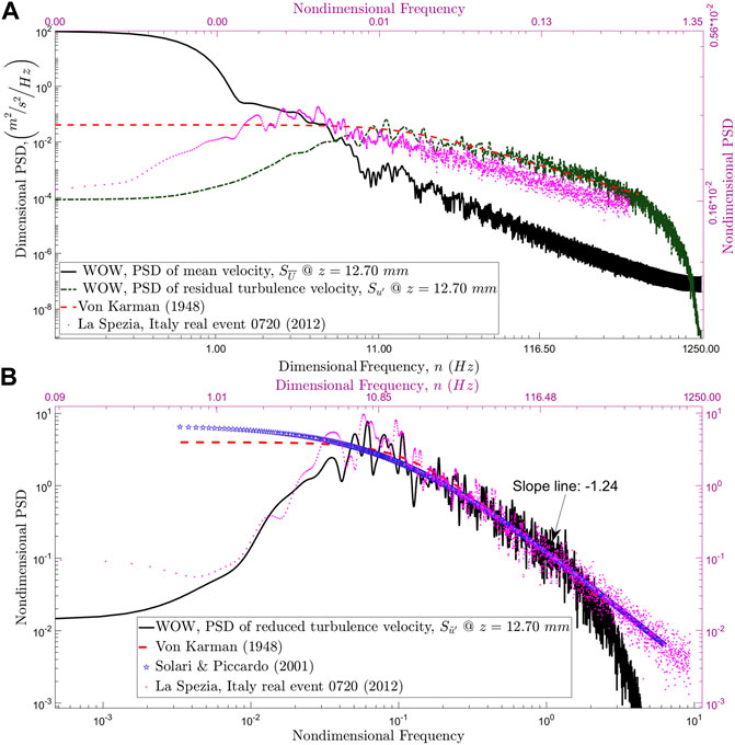
FIGURE 12. Power spectral density (PSD) of the (A) residual and (B) reduced fluctuations for downburst simulators option E at the TTC.

The intersection between the PSD of the residual turbulence and PSD of the moving mean reflects a shedding frequency, $f_{shed}$. It can be seen from Figure 12A that the shedding frequency of the main rolling vortex originated from Option E is 5.76 Hz. If an assumed time scale of 1:5 exists between the small-scale and full-scale downburst simulator at the WOW, then it is estimated that the full-scale downburst simulator will have a shedding frequency of the main rolling vortex of about 1.18 Hz. Fortunately, the duration of the peak zone is a controllable parameter at the WOW as to decide how long the slat opening duration can last. In addition to the PSD analysis, it is also important to compare the probability distribution function (PDF) of the residual $u^{\prime }$ and reduced velocity fluctuations $\stackrel{\sim }{u^{\prime }}$ and estimate the statistical moments that describe their corresponding level of Gaussianity such as mean, standard deviation, skewness, and kurtosis that determine the deviation from a random Gaussian distribution. According to Solari et al. (2015), the reduced velocity fluctuations $\stackrel{\sim }{u^{\prime }}$ can be dealt as a stationary Gaussian random process with zero mean and unit standard deviation as similarly considered in stationary ABL winds. The statistical moments such as mean ${\mu }_{\stackrel{\sim }{u^{\prime }}}$, standard deviation ${\sigma }_{\stackrel{\sim }{u^{\prime }}}$, skewness ${\gamma }_{\stackrel{\sim }{u^{\prime }}}$, and kurtosis ${\kappa }_{\stackrel{\sim }{u^{\prime }}}$ obtained for Option E in the residual fluctuations correspond to 0.001, 1.18, −0.20, and 4.27, respectively, and for the reduced fluctuations the values obtained are −0.007, 0.884, 0.006, and 2.84, respectively. The numbers obtained in the reduced fluctuations closely agree more with the recommended stationary Gaussian values of stationary ABL winds that correspond to be 0, 1, 0, and 3. The statistical moments in the residual fluctuations indicate a non-Gaussian behavior by having high kurtosis and skewness, which the latter is an indication of the offset from the centerline and is negative when shifting toward the right side.

Concluding remarks

Only four downburst simulators out of five designed and tested herein provide a suitable downburst outflow. By adding one of these downburst simulators to a conventional wind tunnel test section, the synoptic winds can be converted into non-stationary winds. Option A offers the design of redirecting the horizontal flow from the wind tunnel facility to a 2-D impinging jet coming vertically downward, hitting the ground and creating the main rolling vortex with a higher peak height $z_{\max }$. Options C, D, or E offer an alternative 2-D wall jet concept that enables the creation of a large-scale main rolling vortex with peak heights that are essential for testing larger scale models. Option B is not recommended because the use of a GG for opening and closing the flow showed inadequate flow characteristics. The incorporation of a gravity gate (GG) in Option E offered a practical, economical, and feasible closing operation. The drawback of the GG is that it increases the acceleration of the ramp-up or ramp-down zones. The selection of a proper time average window $T_{ave}$ for the decomposition of wind velocities in non-stationary and transient events is vital within the peak zone. The global maximum velocity was found in a close vicinity of the downburst slot opening and not obtained in the desired location, which is at the TTC for all tested simulators. However, the vertical velocity profiles still demonstrated a nose shape at the TTC. The increase of surface roughness lengths $z_0$ showed an increase in the peak height $z_{\max }$. It was noticed that the turbulence intensity increases with height, which is in good agreement with previous literature on 2-D wall jets. All the PSD models fitted appropriately in the residual $u^{\prime }$ and the reduced turbulence fluctuations $\stackrel{\sim }{u^{\prime }}$ in Option E. However, it was determined that the most recommended method to analyze and extract turbulence integral length scale near the ground for downbursts is with the use of the PSD on reduced fluctuations. The exponential fit method may need further revisions and modifications to analyze downbursts. It was noticed that the Von Karman model closely fitted the residual and reduced fluctuations in both corresponding PSD analyses for the downburst simulator option E. The PSD of the reduced fluctuation displayed a slope smaller than the −5/3 Kolmogorov’s slope in the inertial subrange. This is expected because of a scaling issue found in the small-scale downburst test. The reduced fluctuations followed statistical characteristics of stationary and Gaussian distribution similarly to ABL stationary winds. All the results and analyses herein indicate that the suggested downburst simulators discussed herein (Options A, C, D, and E) can be used to create downburst outflows with Reynolds numbers reaching up to $R_e=1.22\cdot {10}^4$ in the small-scale WOW EF. The large-scale construction of the recommended downburst simulators will enable the further understanding of wind-induced effects on large-scale structures and the possible codification of transient loading.

Data availability statement

The raw data supporting the conclusion of this article will be made available by the authors, without undue reservation.

Author contributions

The manuscript was prepared by AM and supervised by AE. KV assisted with the experimental procedures, data analysis and collection. DC and AC reviewed the manuscript and helped enhance it.

Funding

These tests were conducted at the NHERI Wall of Wind Experimental Facility (NSF CMMI #1520853 and #2037899). The authors of this manuscript wish to acknowledge the financial support offered by NSF (Award No. 1762968) to perform these tests.

Acknowledgments

The authors of this report wish to thank the WOW personnel, especially Jimmy Erwin, for their continuous assistance and support.

Conflict of interest

The authors declare that the research was conducted in the absence of any commercial or financial relationships that could be construed as a potential conflict of interest.

Publisher’s note

All claims expressed in this article are solely those of the authors and do not necessarily represent those of their affiliated organizations, or those of the publisher, the editors, and the reviewers. Any product that may be evaluated in this article, or claim that may be made by its manufacturer, is not guaranteed or endorsed by the publisher.

References

Abd-Elaal, E.-S., Mills, J. E., and Ma, X. (2018). Numerical simulation of downburst wind flow over real topography. J. Wind Eng. Ind. Aerodyn. 172, 85–95.
CrossRef Full Text | Google Scholar
Abdelwahab, M., Ghazal, T., and Aboshosha, H. (2022). Designing a multi-purpose wind tunnel suitable for limited spaces. Results Eng. 14, 100458. doi:10.1016/j.rineng.2022.100458
Aboshosha, H., Bitsuamlak, G., and El Damatty, A. (2015). Turbulence characterization of downbursts using LES. J. Wind Eng. Industrial Aerodynamics 136, 44–61. doi:10.1016/j.jweia.2014.10.020
Aboshosha, H. (2014). Response of transmission line conductors under downburst wind. London, ON: The University of Western Ontario.
Google Scholar
Aboutabikh, M., Ghazal, T., Chen, J., Elgamal, S., and Aboshosha, H. (2019). Designing a blade-system to generate downburst outflows at boundary layer wind tunnel. J. Wind Eng. Industrial Aerodynamics 186, 169–191. doi:10.1016/j.jweia.2019.01.005
Alahyari, A., and Longmire, E. K. (1994). Particle image velocimetry in a variable density flow: Application to a dynamically evolving microburst. Exp. Fluids 17, 434–440. doi:10.1007/bf01877047
Antoniou, I., Asimakopoulos, D., Fragoulis, A., Kotronaros, A., Lalas, D., and Panourgias, I. (1992). Turbulence measurements on top of a steep hill. J. Wind Eng. Industrial Aerodynamics 39, 343–355. doi:10.1016/0167-6105(92)90558-r
Asano, K., Iida, Y., and Uematsu, Y. (2019). Laboratory study of wind loads on a low-rise building in a downburst using a moving pulsed jet simulator and their comparison with other types of simulators. J. Wind Eng. Industrial Aerodynamics 184, 313–320. doi:10.1016/j.jweia.2018.11.034
Bolgiani, P., Santos-Muñoz, D., Fernández-González, S., Sastre, M., Valero, F., and Martin, M. L. (2020). Microburst detection with the WRF model: Effective resolution and forecasting indices. JGR. Atmos. 125, e2020JD032883. doi:10.1029/2020jd032883
Butler, K., and Kareem, A. (2007). “Physical and numerical modeling of downburst generated gust fronts,” in Proceedings of the 12th international conference on wind engineering (Cairns, Australia: IEEE).
Cao, S., Nishi, A., Kikugawa, H., and Matsuda, Y. (2002). Reproduction of wind velocity history in a multiple fan wind tunnel. J. Wind Eng. Industrial Aerodynamics 90, 1719–1729. doi:10.1016/s0167-6105(02)00282-9
Chay, M. T., and Letchford, C. W. (2002). Pressure distributions on a cube in a simulated thunderstorm downburst—Part A: Stationary downburst observations. J. Wind Eng. Industrial Aerodynamics 90, 711–732. doi:10.1016/s0167-6105(02)00158-7
Chay, M. T. (2001). Physical modeling of thunderstorm downbursts for wind engineering applications. Lubbock, TX: Texas Tech University.
Chen, L., and Letchford, C. W. (2004). A deterministic–stochastic hybrid model of downbursts and its impact on a cantilevered structure. Eng. Struct. 26, 619–629. doi:10.1016/j.engstruct.2003.12.009
Choi, E. C. C., and Hidayat, F. A. (2002). Gust factors for thunderstorm and non-thunderstorm winds. J. Wind Eng. Industrial Aerodynamics 90, 1683–1696. doi:10.1016/s0167-6105(02)00279-9
Chowdhury, A. G., Vutukuru, K. S., and Moravej, M. (2018). Full-and large-scale experimentation using the wall of wind to mitigate wind loading and rain impacts on buildings and infrastructure systems. Available at: https://www.academia.edu/43153499/Full_and_Large_Scale_Experimentation_Using_the_Wall_of_Wind_to_Mitigate_Wind_Loading_and_Rain_Impacts_on_Buildings_and_Infrastructure_Systems.
Chowdhury, A., Zisis, I., Irwin, P., Bitsuamlak, G., Pinelli, J. P., Hajra, B., et al. (2017). Large-scale experimentation using the 12-fan wall of wind to assess and mitigate hurricane wind and rain impacts on buildings and infrastructure systems. J. Struct. Eng. 143, 4017053. doi:10.1061/(asce)st.1943-541x.0001785
Davenport, A. G. (1961). The spectrum of horizontal gustiness near the ground in high winds. Q. J. R. Meteorol. Soc. 87, 194–211. doi:10.1002/qj.49708737208
Dunsavage, J. (2020). Evolving risks call for innovation to reduce costs. Drive Resil. 2020, 1–15.
Elawady, A., Aboshosha, H., El Damatty, A., Bitsuamlak, G., Hangan, H., and Elatar, A. (2017). Aero-elastic testing of multi-spanned transmission line subjected to downbursts. J. Wind Eng. Industrial Aerodynamics 169, 194–216. doi:10.1016/j.jweia.2017.07.010
Eurocode, B. (2005). Eurocode 1: Actions on structures–part1-4: General actions-wind actions; BS EN 1991-1-4: 2005. London: Br. Stand. Institution.
Fujita, T. (1990). Downbursts: Meteorological features and wind field characteristics. J. Wind Eng. Industrial Aerodynamics 36, 75–86. doi:10.1016/0167-6105(90)90294-m
Fujita, T. T. (1986). DFW (Dallas-Ft. Worth) microburst on august 2, 1985. Chicago, IL, United States: Chicago Univ.
Fujita, T. T. (1985). The downburst. SMRP 210, 112.
Fujita, T. T. (1981). Tornadoes and downbursts in the context of generalized planetary scales. J. Atmos. Sci. 38, 1511–1534. doi:10.1175/1520-0469(1981)038<1511:taditc>2.0.co;2
Hangan, H., Kim, J.-D., and Xu, Z. (2004). “The simulation of downbursts and its challenges,” in Structures 2004: Building on the past, securing the future (Springer), 1–8.
Hangan, H., Refan, M., Jubayer, C., Romanic, D., Parvu, D., LoTufo, J., et al. (2017). Novel techniques in wind engineering. J. Wind Eng. Industrial Aerodynamics 171, 12–33. doi:10.1016/j.jweia.2017.09.010
Harris, R. I. (1968). Measurements of wind structure at heights up to 598 ft above ground level. England, United Kingdom: Electrical Research Association.
Hjelmfelt, M. R. (1988). Structure and life cycle of microburst outflows observed in Colorado. J. Appl. Meteor. 27, 900–927. doi:10.1175/1520-0450(1988)027<0900:salcom>2.0.co;2
Hjelmfelt, M. R. (2002). Structure and life cycle of microburst outflows observed in Colorado. J. Appl. Meteor. 27, 900–927. doi:10.1175/1520-0450(1988)027<0900:salcom>2.0.co;2
Holmes, J. D., Hangan, H. M., Schroeder, J. L., Letchford, C. W., and Orwig, K. D. (2008). A forensic study of the Lubbock-Reese downdraft of 2002. Wind Struct. 11, 137–152. doi:10.12989/was.2008.11.2.137
Holmes, J. D. (1999). “Modeling of extreme thunderstorm winds for wind loading of structures and risk assessment,” inWind Engineering into the 21st Century, Proceedings of the 10th International Conference on Wind Engineering, Copenhagen, Denmark, 1409–1415.
Holmes, J. D., and Oliver, S. E. (2000). An empirical model of a downburst. Eng. Struct. 22, 1167–1172. doi:10.1016/s0141-0296(99)00058-9
Holmes, J. D. (1992). “Physical modelling of thunderstorm downdrafts by wind tunnel jet,” in 2nd AWES workshop (Victoria, Australia: Monash University), 29–32.
Hoogewind, K. A., Baldwin, M. E., and Trapp, R. J. (2017). The impact of climate change on hazardous convective weather in the United States: Insight from high-resolution dynamical downscaling. J. Clim. 30, 10081–10100. doi:10.1175/jcli-d-16-0885.1
Huang, G. (2015). Application of proper orthogonal decomposition in fast Fourier transform—Assisted multivariate nonstationary process simulation. J. Eng. Mech. 141, 4015015. doi:10.1061/(asce)em.1943-7889.0000923
Huang, G., Zheng, H., Xu, Y., and Li, Y. (2015). Spectrum models for nonstationary extreme winds. J. Struct. Eng. 141, 4015010. doi:10.1061/(asce)st.1943-541x.0001257
Ivan, M. (1986). A ring-vortex downburst model for flight simulations. J. Aircr. 23, 232–236. doi:10.2514/3.45294
Jesson, M., Sterling, M., Letchford, C., and Haines, M. (2015). Aerodynamic forces on generic buildings subject to transient, downburst-type winds. J. Wind Eng. Industrial Aerodynamics 137, 58–68. doi:10.1016/j.jweia.2014.12.003
Jubayer, C., Elatar, A., and Hangan, H. (2016). “Pressure distributions on a low-rise building in a laboratory simulated downburst,” in Proceedings of the 8th international colloquium on bluff body aerodynamics and applications (Boston, Massachusetts, USA: IEEE).
Junayed, C., Jubayer, C., Parvu, D., Romanic, D., and Hangan, H. (2019). Flow field dynamics of large-scale experimentally produced downburst flows. J. Wind Eng. Industrial Aerodynamics 188, 61–79. doi:10.1016/j.jweia.2019.02.008
Kaimal, J. C., Wyngaard, J. C. J., Izumi, Y., and Coté, O. R. (1972). Spectral characteristics of surface-layer turbulence. Q. J. R. Meteorol. Soc. 98, 563–589. doi:10.1002/qj.49709841707
Kim, J., Hangan, H., and Eric Ho, T. C. (2007). Downburst versus boundary layer induced wind loads for tall buildings. Wind Struct. 10, 481–494. doi:10.12989/was.2007.10.5.481
Kim, J., and Hangan, H. (2007). Numerical simulations of impinging jets with application to downbursts. J. Wind Eng. Industrial Aerodynamics 95, 279–298. doi:10.1016/j.jweia.2006.07.002
Knowles, K., and Myszko, M. (1998). Turbulence measurements in radial wall-jets. Exp. Therm. Fluid Sci. 17, 71–78. doi:10.1016/s0894-1777(97)10051-6
Landreth, C. C., and Adrian, R. J. (1990). Impingement of a low Reynolds number turbulent circular jet onto a flat plate at normal incidence. Exp. Fluids 9, 74–84. doi:10.1007/bf00575338
Launder, B. E., and Rodi, W. (1983). The turbulent wall jet measurements and modeling. Annu. Rev. Fluid Mech. 15, 429–459. doi:10.1146/annurev.fl.15.010183.002241
Le, V., and Caracoglia, L. (2020). Experimental investigation on non-stationary wind loading effects generated with a multi-blade flow device. J. Fluids Struct. 96, 103049. doi:10.1016/j.jfluidstructs.2020.103049
Le, V., and Caracoglia, L. (2019). Generation and characterization of a non-stationary flow field in a small-scale wind tunnel using a multi-blade flow device. J. Wind Eng. Industrial Aerodynamics 186, 1–16. doi:10.1016/j.jweia.2018.12.017
Letchford, C., and Illidge, G. (1999). “Turbulence and topographic effects in simulated downrafts by wind tunnel jet,” in Proceedings of the 10th international conference on wind engineering, copenhagen, Denmark, 21-24 june 1999 (Netherlands: Rotterdam).
Letchford, C. W., and Chay, M. T. (2002). Pressure distributions on a cube in a simulated thunderstorm downburst. Part B: Moving downburst observations. J. Wind Eng. Industrial Aerodynamics 90, 733–753. doi:10.1016/s0167-6105(02)00163-0
Letchford, C. W., Mans, C., and Chay, M. T. (2002). Thunderstorms—Their importance in wind engineering (a case for the next generation wind tunnel). J. Wind Eng. Industrial Aerodynamics 90, 1415–1433. doi:10.1016/s0167-6105(02)00262-3
Li, C., Li, Q. S., Xiao, Y. Q., and Ou, J. P. (2012). A revised empirical model and CFD simulations for 3D axisymmetric steady-state flows of downbursts and impinging jets. J. Wind Eng. Industrial Aerodynamics 102, 48–60. doi:10.1016/j.jweia.2011.12.004
Lin, W. E., Orf, L. G., Savory, E., and Novacco, C. (2007). Proposed large-scale modelling of the transient features of a downburst outflow. Wind Struct. 10, 315–346. doi:10.12989/was.2007.10.4.315
Lin, W. E., and Savory, E. (2010). Physical modelling of a downdraft outflow with a slot jet. Wind Struct. an Int. J. 13, 385–412. doi:10.12989/was.2010.13.5.385
Lin, W. E. (2010). Validation of a novel downdraff outflow simulator. A slot jet wind tunnel Ottawa, Canada: Library and Archives.
Lin, W., Mara, T., and Savory, E. (2015). “Wind velocity profiles from a pulsed wall jet over ground roughness,” in 14th international conference on wind engineering (Brazil: Porto Alegre), 1–16.
Lin, W. E. (2012). Validation of a novel downdraft outflow simulator: A slot jet wind tunnel. Ottawa, ON: Library and Archives
Lin, W., and Savory, E. (2006). Large-scale quasi-steady modelling of a downburst outflow using a slot jet. Wind Struct. 9, 419–440. doi:10.12989/was.2006.9.6.419
Lombardo, F. T., Mason, M. S., and de Alba, A. Z. (2018). Investigation of a downburst loading event on a full-scale low-rise building. J. Wind Eng. Industrial Aerodynamics 182, 272–285. doi:10.1016/j.jweia.2018.09.020
Lundgren, T. S., Yao, J., and Mansour, N. N. (1992). Microburst modelling and scaling. J. Fluid Mech. 239, 461–488. doi:10.1017/s002211209200449x
Makita, H. (1991). Realization of a large-scale turbulence field in a small wind tunnel. Fluid Dyn. Res. 8, 53–64. doi:10.1016/0169-5983(91)90030-m
Mason, M. S., Fletcher, D. F., and Wood, G. S. (2010). Numerical simulation of idealised three-dimensional downburst wind fields. Eng. Struct. 32, 3558–3570. doi:10.1016/j.engstruct.2010.07.024
Mason, M. S., Letchford, C. W., and James, D. L. (2005). Pulsed wall jet simulation of a stationary thunderstorm downburst, Part A: Physical structure and flow field characterization. J. Wind Eng. Industrial Aerodynamics 93, 557–580. doi:10.1016/j.jweia.2005.05.006
Mason, M. S., Wood, G. S., and Fletcher, D. F. (2007). Impinging jet simulation of stationary downburst flow over topography. Wind Struct. 10, 437–462. doi:10.12989/was.2007.10.5.437
Mason, M. S., Wood, G. S., and Fletcher, D. F. (2009b). Influence of tilt and surface roughness on the outflow wind field of an impinging jet. Wind Struct. an Int. J. 12, 179–204. doi:10.12989/was.2009.12.3.179
Mason, M. S., Wood, G. S., and Fletcher, D. F. (2009a). Numerical simulation of downburst winds. J. Wind Eng. Industrial Aerodynamics 97, 523–539. doi:10.1016/j.jweia.2009.07.010
Matsumoto, M. (2007). “Drag forces on 2-D cylinders due to sudden increase of wind velocity,” in Proceedings of 12th international conference on wind engineering (IEEE), 1727–1734.
Matsumoto, M. (1984). Study on unsteady aerodynamic in unsteady wind flow. Kyoto, Japan: Kyoto University.
McConville, A. C., Sterling, M., and Baker, C. J. (2009). The physical simulation of thunderstorm downbursts using an impinging jet. Wind Struct. an Int. J. 12, 133–149. doi:10.12989/was.2009.12.2.133
McCullough, M., Kwon, D. K., Kareem, A., and Wang, L. (2014). Efficacy of averaging interval for nonstationary winds. J. Eng. Mech. 140, 1–19. doi:10.1061/(asce)em.1943-7889.0000641
Moghim, F., Xia, F. T., and Caracoglia, L. (2015). Experimental analysis of a stochastic model for estimating wind-borne compact debris trajectory in turbulent winds. J. Fluids Struct. 54, 900–924. doi:10.1016/j.jfluidstructs.2015.02.007
NOAA (2018). National oceanic and atmospheric administration, office for coastal management. Available at: https://www.noaa.gov/.
O’Donovan, T. S. (2005). Fluid flow and heat transfer of an impinging air jet.&hairsp; Dublin, Ireland: Univ. Dublin.
Oseguera, R. M., and Bowles, R. L. (1988). A simple, analytic 3-dimensional downburst model based on boundary layer stagnation flow. Available at: https://ntrs.nasa.gov/api/citations/19880018674/downloads/19880018674.pdf.
Peng, L., Huang, G., Chen, X., and Kareem, A. (2017). Simulation of multivariate nonstationary random processes: Hybrid stochastic wave and proper orthogonal decomposition approach. J. Eng. Mech. 143, 4017064. doi:10.1061/(asce)em.1943-7889.0001273
Proctor, F. H. (1988). Numerical simulations of an isolated microburst. Part I: Dynamics and structure. J. Atmos. Sci. 45, 3137–3160. doi:10.1175/1520-0469(1988)045<3137:nsoaim>2.0.co;2
Proctor, F. H. (1989). Numerical simulations of an isolated microburst. Part II: Sensitivity experiments. J. Atmos. Sci. 46, 2143–2165. doi:10.1175/1520-0469(1989)046<2143:nsoaim>2.0.co;2
Repetto, M. P., Burlando, M., Solari, G., De Gaetano, P., Pizzo, M., and Tizzi, M. (2018). A web-based GIS platform for the safe management and risk assessment of complex structural and infrastructural systems exposed to wind. Adv. Eng. Softw. 117, 29–45. doi:10.1016/j.advengsoft.2017.03.002
Richter, A., Ruck, B., Mohr, S., and Kunz, M. (2018). Interaction of severe convective gusts with a street canyon. Urban Clim. 23, 71–90. doi:10.1016/j.uclim.2016.11.003
Romanic, D., Chowdhury, J., Jubayer, C., and Hangan, H. (2020). Investigation of the transient nature of thunderstorm winds from Europe, the United States, and Australia using a new method for detection of changepoints in wind speed records. Mon. Weather Rev. 148, 3747–3771.
Sarkar, P. P., Haan Fred, L, J., Balaramudu, V., and Sengupta, A. (2006). “Laboratory simulation of tornado and microburst to assess wind loads on buildings,” in Structures congress 2006: Structural engineering and public safety (Springer), 1–10.
Sassa, K., Inoue, A., and Miyagi, H. (2009). “Gust fronts generated in a multi-fan wind tunnel,” in The seventh asia-pacific conference on wind engineering (Taipei, Taiwan: IAWE).
Selvam, R. P., and Holmes, J. D. (1992). Numerical simulation of thunderstorm downdrafts. J. Wind Eng. Industrial Aerodynamics 44, 2817–2825. doi:10.1016/0167-6105(92)90076-m
Sengupta, A., and Sarkar, P. P. (2008). Experimental measurement and numerical simulation of an impinging jet with application to thunderstorm microburst winds. J. Wind Eng. Industrial Aerodynamics 96, 345–365. doi:10.1016/j.jweia.2007.09.001
Simiu, E., and Scanlan, R. H. (1978). Wind effects on structures. Wiley.
Solari, G., Burlando, M., De Gaetano, P., and Repetto, M. P. (2015). Characteristics of thunderstorms relevant to the wind loading of structures. Wind Struct. 20, 763–791. doi:10.12989/was.2015.20.6.763
Solari, G. (1993). Gust buffeting. II: Dynamic alongwind response. J. Struct. Eng. 119, 383–398. doi:10.1061/(asce)0733-9445(1993)119:2(383)
Solari, G. (2018). “Mixed climatology, non-synoptic phenomena and downburst wind loading of structures,” in Conference of the Italian association for wind engineering (Springer), 17–31.
Solari, G., and Piccardo, G. (2001). Probabilistic 3-D turbulence modeling for gust buffeting of structures. Probabilistic Eng. Mech. 16, 73–86. doi:10.1016/s0266-8920(00)00010-2
Solari, G., Rainisio, D., and De Gaetano, P. (2017). Hybrid simulation of thunderstorm outflows and wind-excited response of structures. Meccanica 52, 3197–3220. doi:10.1007/s11012-017-0718-x
Solari, G., Repetto, M. P., Burlando, M., De Gaetano, P., Pizzo, M., Tizzi, M., et al. (2012). The wind forecast for safety management of port areas. J. Wind Eng. Industrial Aerodynamics 104, 266–277. doi:10.1016/j.jweia.2012.03.029
Solari, G. (2016). Thunderstorm response spectrum technique: Theory and applications. Eng. Struct. 108, 28–46. doi:10.1016/j.engstruct.2015.11.012
Teunissen, H. W. (1980). Structure of mean winds and turbulence in the planetary boundary layer over rural terrain. Bound. Layer. Meteorol. 19, 187–221. doi:10.1007/bf00117220
Van Hooff, T., Blocken, B., Defraeye, T., Carmeliet, J., and Van Heijst, G. J. F. (2012). PIV measurements of a plane wall jet in a confined space at transitional slot Reynolds numbers. Exp. Fluids 53, 499–517. doi:10.1007/s00348-012-1305-5
Verhoff, A. (1963). The two-dimensional, turbulent wall jet with and without an external free stream. Princeton, NJ: Princeton Univ NJ.
Vermeire, B. C., Orf, L. G., and Savory, E. (2011). A parametric study of downburst line near-surface outflows. J. Wind Eng. Industrial Aerodynamics 99, 226–238. doi:10.1016/j.jweia.2011.01.019
Vicroy, D. D. (1992). Assessment of microburst models for downdraft estimation. J. Aircr. 29, 1043–1048. doi:10.2514/3.46282
Von Karman, T. (1948). Progress in the statistical theory of turbulence. Proc. Natl. Acad. Sci. U. S. A. 34, 530–539. doi:10.1073/pnas.34.11.530
Walker, J. D. A., Smith, C. R., Cerra, A. W., and Doligalski, T. L. (1987). The impact of a vortex ring on a wall. J. Fluid Mech. 181, 99–140. doi:10.1017/s0022112087002027
Wang, L., and Kareem, A. (2004). “Modeling of non-stationary winds in gust-fronts,” in 9th ASCE specialty conference on probabilistic mechanics and structural reliability (American Society of Civil Engineers, Sandia National Laboratories), 1–6.
Wang, L., McCullough, M., and Kareem, A. (2013). A data-driven approach for simulation of full-scale downburst wind speeds. J. Wind Eng. Industrial Aerodynamics 123, 171–190. doi:10.1016/j.jweia.2013.08.010
Wang, L., McCullough, M., and Kareem, A. (2014). Modeling and simulation of nonstationary processes utilizing wavelet and Hilbert transforms. J. Eng. Mech. 140, 345–360. doi:10.1061/(asce)em.1943-7889.0000666
Wood, G. S., Kwok, K. C. S., Motteram, N. A., and Fletcher, D. F. (2001). Physical and numerical modelling of thunderstorm downbursts. J. Wind Eng. Industrial Aerodynamics 89, 535–552. doi:10.1016/s0167-6105(00)00090-8
Xu, Z., and Hangan, H. (2008). Scale, boundary and inlet condition effects on impinging jets. J. Wind Eng. Industrial Aerodynamics 96, 2383–2402. doi:10.1016/j.jweia.2008.04.002
Xu, Z., Hangan, H., and Yu, P. (2008). Analytical solutions for a family of Gaussian impinging jets. J. Appl. Mech. 75, 21019. doi:10.1115/1.2775502
Zhang, S., Yang, Q., Solari, G., Li, B., and Huang, G. (2019). Characteristics of thunderstorm outflows in Beijing urban area. J. Wind Eng. Industrial Aerodynamics 195, 104011. doi:10.1016/j.jweia.2019.104011
Zhang, Y., Hu, H., and Sarkar, P. P. (2014). Comparison of microburst-wind loads on low-rise structures of various geometric shapes. J. Wind Eng. Industrial Aerodynamics 133, 181–190. doi:10.1016/j.jweia.2014.06.012
Zhang, Y., Hu, H., and Sarkar, P. P. (2013a). Modeling of microburst outflows using impinging jet and cooling source approaches and their comparison. Eng. Struct. 56, 779–793. doi:10.1016/j.engstruct.2013.06.003
Zhang, Y., Sarkar, P., and Hu, H. (2013b). An experimental study of flow fields and wind loads on gable-roof building models in microburst-like wind. Exp. Fluids 54, 1511. doi:10.1007/s00348-013-1511-9
Zhao, Y., Cao, S., Tamura, Y., Duan, Z., and Ozono, S. (2009). “Simulation of downburst in a multiple fan wind tunnel and research on its load on high-rise structure by wind tunnel experiment,” in 2009 international conference on mechatronics and automation (IEEE), 4506–4511.
Zhu, S., and Etkin, B. (1985). Model of the wind field in a downburst. J. Aircr. 22, 595–601. doi:10.2514/3.45171
Keywords: downburst, thunderstorm, wind tunnel testing, wall of wind, non-synoptic wind
Citation: Mejia AD, Elawady A, Vutukuru KS, Chen D and Chowdhury AG (2022) Examination of different wall jet and impinging jet concepts to produce large-scale downburst outflow. Front. Built Environ. 8:980617. doi: 10.3389/fbuil.2022.980617
Received: 28 June 2022; Accepted: 16 August 2022;
Published: 27 September 2022.
Edited by:
Sukanta Basu, Delft University of Technology, Netherlands
Reviewed by:
Haitham Aboshosha, Ryerson University, Canada
Arnab Sarkar, Indian Institute of Technology (BHU), India
Copyright © 2022 Mejia, Elawady, Vutukuru, Chen and Chowdhury. This is an open-access article distributed under the terms of the Creative Commons Attribution License (CC BY). The use, distribution or reproduction in other forums is permitted, provided the original author(s) and the copyright owner(s) are credited and that the original publication in this journal is cited, in accordance with accepted academic practice. No use, distribution or reproduction is permitted which does not comply with these terms.
*Correspondence: Alvaro Danilo Mejia, ameji023@fiu.edu
Present address:Krishna Sai Vutukuru, Thornton Tomasetti, Fort Lauderdale, FL, United States