A New Method for Numerical Integration of Higher-Order Ordinary Differential Equations Without Losing the Periodic Responses

Katsikadelis, John T.

doi:10.3389/fbuil.2021.621037

ORIGINAL RESEARCH article

Front. Built Environ., 22 April 2021
Sec. Computational Methods in Structural Engineering
Volume 7 - 2021 | https://doi.org/10.3389/fbuil.2021.621037

A New Method for Numerical Integration of Higher-Order Ordinary Differential Equations Without Losing the Periodic Responses

John T. Katsikadelis^*

School of Civil Engineering, National Technical University of Athens, Athens, Greece

A new numerical method is presented for the solution of initial value problems described by systems of N linear ordinary differential equations (ODEs). Using the state-space representation, a differential equation of order n > 1 is transformed into a system of L = n×N first-order equations, thus the numerical method developed recently by Katsikadelis for first-order parabolic differential equations can be applied. The stability condition of the numerical scheme is derived and is investigated using several well-corroborated examples, which demonstrate also its convergence and accuracy. The method is simply implemented. It is accurate and has no numerical damping. The stability does not require symmetrical and positive definite coefficient matrices. This advantage is important because the scheme can find the solution of differential equations resulting from methods in which the space discretization does not result in symmetrical matrices, for example, the boundary element method. It captures the periodic behavior of the solution, where many of the standard numerical methods may fail or are highly inaccurate. The present method also solves equations having variable coefficients as well as non-linear ones. It performs well when motions of long duration are considered, and it can be employed for the integration of stiff differential equations as well as equations exhibiting softening where widely used methods may not be effective. The presented examples demonstrate the efficiency and accuracy of the method.

1. Introduction

The great majority of problems in engineering and mathematical physics are described by first-order (parabolic) and second-order (hyperbolic) differential equations, modeling the diffusion in bodies, the motion of systems, and other responses. A reason that equations of order higher than the second do not appear often is that many classical mathematical models of the physical world are derived from Newton's law of motion. However, there are many phenomena in engineering, physics, and biology that are described by higher-order equations, e.g., the entry-flow, the variation of the thyroid hormone, and several other phenomena are described by third-order differential equations (Padhi and Pati, 2014). Plenty of analytical methods have been developed for solving higher-order ordinary differential equations (ODEs) of a specific form. Many efficient numerical methods have also been developed for solving such equations with the Runge–Kutta method and its modifications playing an essential role (Butcher, 2000, 2008). Therefore, the question of why to develop a new numerical method to solve such equations looks plausible. The answer comes from the following fact. In recent years, the use of differential models to describe the dynamic response of viscoelastic structures leads to discrete ODEs of order higher than two, whose solution exhibits periodic behavior (Nerantzaki and Babouskos, 2012; Katsikadelis, 2014, 2016a). It is known that the periodic response cannot be captured by the available numerical methods (Simos, 1997) unless they are symmetric or are adapted to a specific problem. Otherwise, they lead to inaccurate results. Actually, the motivation for developing the present method mainly was to cope with such problems. The proposed method solves efficiently and accurately these equations, and it is problem-independent.

The initial value problem (IVP) for the n > 0 order linear ODE is stated as:

\begin{array}{l} y^{(n)} + a_{1} y^{(n - 1)} + a_{2} y^{(n - 2)} + \dots + a_{n - 1} y^{'} + a_{n} y = f (t), \\ t \in [0, T], T > 0 & (1.1a) \end{array}

\begin{array}{l} y (0) = y_{0}, y^{'} (0) = y_{0}^{'}, y^{″} (0) = y_{0}^{″}, \dots, y^{(n - 1)} (0) \\ = y_{0}^{(n - 1)} & (1.1b) \end{array}

where, a₁, a₂, … a_n−1, a_n are N × N real matrices, $y = y (t) = {\begin{matrix} y_{1} (t) & y_{2} (t) & \dots & y_{n} (t) \end{matrix}}^{T}$ is the vector of the unknown functions, $f (t) = {\begin{matrix} f_{1} (t) & f_{2} (t) & \dots & f_{n} (t) \end{matrix}}^{T}$ the vector of external sources, and $y_{0}, y_{0}^{'}, y_{0}^{″}, \dots, y_{0}^{(n - 1)}$ are N × 1 given vectors representing the initial conditions.

In the presented method, the systems of N linear ODEs (1.1a) is transformed into a system of L = n × N first-order ODEs, which is subsequently solved using the numerical method developed by Katsikadelis for systems of first-order ODEs (Katsikadelis, 2016b). The latter method is based on the principle of the analog equation, which converts the L coupled first-order ODEs equations into a set of L single term uncoupled first-order ODEs with fictitious sources.

The investigation of the stability of the numerical scheme results in the condition that the coefficient matrices of the equation must satisfy. Besides, well-corroborated numerical examples show the accuracy and convergence of the method. The method is simply implemented, self-starting, and accurate. The stability does not demand symmetrical and positive definite coefficient matrices a₁, a₂, … a_n−1, a_n. This advantage is important because the scheme can find the solution of differential equations resulting from methods in which the space discretization does not result in symmetrical coefficient matrices but only satisfies the stability condition, for example, the boundary element method. Moreover, it captures the periodic behavior of the solution, where many of the standard numerical methods may be ineffective or highly inaccurate. The present method also solves equations having variable coefficients, i.e., a₁(t), a₂(t), … a_n−1(t), a_n(t), as well as non-linear ones. The efficiency of the method is illustrated by solving several equations, including linear and non-linear benchmark ODEs.

2. Linear Equations

The n-th Order Linear ODE

We consider now the n-th order ODE, Equation (1.1). If we set:

\begin{array}{l} x_{1} = y \\ x_{2} = {x^{'}}_{1} = y^{'} \\ x_{3} = {x^{'}}_{2} = y^{″} \\ \dots = \dots \dots \dots \\ x_{n} = {x^{'}}_{n - 1} = y^{(n - 1)} & (2.1) \end{array}

Equation (2.1) is reduced to the system of L = n × N first-order ODEs:

\begin{array}{l} [\begin{matrix} I & 0 & 0 & \dots & 0 & 0 \\ 0 & I & 0 & \dots & 0 & 0 \\ 0 & 0 & I & \dots & 0 & 0 \\ ⋮ & ⋮ & ⋮ & ⋱ & ⋮ & ⋮ \\ 0 & 0 & 0 & \dots & I & 0 \\ 0 & 0 & 0 & \dots & 0 & I \end{matrix}] {\begin{matrix} {x^{'}}_{1} \\ {x^{'}}_{2} \\ {x^{'}}_{3} \\ ⋮ \\ {x^{'}}_{n - 1} \\ {x^{'}}_{n} \end{matrix}} \\ + [\begin{matrix} 0 & - I & 0 & \dots & 0 & 0 \\ 0 & 0 & - I & \dots & 0 & 0 \\ 0 & 0 & 0 & \dots & 0 & 0 \\ ⋮ & ⋮ & ⋮ & ⋱ & ⋮ & ⋮ \\ 0 & 0 & 0 & \dots & 0 & - I \\ a_{n} & a_{n - 1} & a_{n - 2} & \dots & a_{2} & a_{1} \end{matrix}] {\begin{matrix} x_{1} \\ x_{2} \\ x_{3} \\ ⋮ \\ x_{n - 1} \\ x_{n} \end{matrix}} = {\begin{matrix} 0 \\ 0 \\ 0 \\ ⋮ \\ 0 \\ f \end{matrix}} & (2.2) \end{array}

Equation (2.2) is of the form:

\begin{array}{l} C \dot{u} + K u = p & (2.3) \end{array}

where now,

\begin{array}{l} C = {[\begin{matrix} I & 0 & 0 & \dots & 0 & 0 \\ 0 & I & 0 & \dots & 0 & 0 \\ 0 & 0 & I & \dots & 0 & 0 \\ ⋮ & ⋮ & ⋮ & ⋱ & ⋮ & ⋮ \\ 0 & 0 & 0 & \dots & I & 0 \\ 0 & 0 & 0 & \dots & 0 & I \end{matrix}]}_{L \times L} K = {[\begin{matrix} 0 & - I & 0 & \dots & 0 & 0 \\ 0 & 0 & - I & \dots & 0 & 0 \\ 0 & 0 & 0 & \dots & 0 & 0 \\ ⋮ & ⋮ & ⋮ & ⋱ & ⋮ & ⋮ \\ 0 & 0 & 0 & \dots & 0 & - I \\ a_{n} & a_{n - 1} & a_{n - 2} & \dots & a_{2} & a_{1} \end{matrix}]}_{L \times L} & (2.4a,b) \end{array}

\begin{array}{l} u = {\begin{matrix} x_{1} \\ x_{2} \\ x_{3} \\ ⋮ \\ x_{n - 1} \\ x_{n} \end{matrix}}_{L \times 1} p = {\begin{matrix} 0 \\ 0 \\ 0 \\ ⋮ \\ 0 \\ f \end{matrix}}_{L \times 1} & (2.4c,d) \end{array}

Then, the method presented in Katsikadelis (2016b) is used to solve Equation (2.3) with initial conditions.

\begin{array}{l} u_{0} = {\begin{matrix} x_{1} (0) \\ x_{2} (0) \\ x_{3} (0) \\ ⋮ \\ x_{n - 1} (0) \\ x_{n} (0) \end{matrix}} = {\begin{matrix} y_{0} \\ {y^{'}}_{0} \\ {y^{″}}_{0} \\ ⋮ \\ y_{0}^{(n - 2)} \\ y_{0}^{(n - 1)} \end{matrix}}_{L \times 1} & (2.5) \end{array}

Table 1 shows the solution algorithm.

TABLE 1

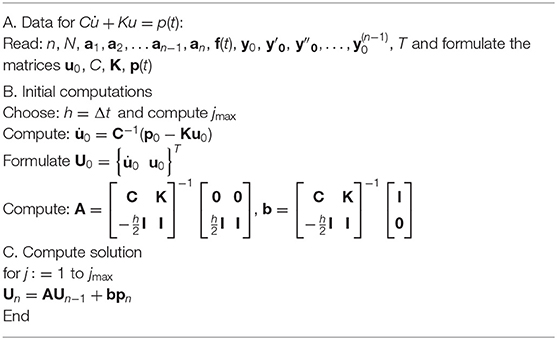
Table 1. Algorithm for the numerical solution of the linear equations n-th order ODEs in the interval [0, T].

Stability of the Numerical Scheme

As it was proved in Katsikadelis (2016b), the numerical scheme in Table 1 is stable if all eigenvalues λ_i of the matrix K have a non-negative real part. In the following, it is proved that this condition is satisfied if the N roots of the n-th order polynomial,

\begin{array}{l} Π (λ) = I λ^{n} - A_{1} λ^{(n - 1)} + A_{2} λ^{(n - 2)} - \dots + {(- 1)}^{n} A_{N} & (2.6) \end{array}

have a non-negative real part. A₁, A₂, ⋯ , A_N are the diagonal matrices of the eigenvalues of a₁, a₂, … a_n−1, a_n.

Proof

According to Katsikadelis (2016b), the numerical scheme is stable if the eigenvalues of the matrix $\hat{K} = C^{- 1} K$ , where C and K are defined by Equations (2.4a,b), have a non-negative real part. Apparently, since C = I, it is $\hat{K} = K$ . For convenience, we illustrate the proof with second-order ODE. Then, the proof is easily extended to the n-th order ODE.

For the second order ODE, it is:

\begin{array}{l} K = [\begin{matrix} 0 & - I \\ a_{2} & a_{1} \end{matrix}] & (2.7) \end{array}

The pertinent eigenvalue problem for K is:

\begin{array}{l} [\begin{matrix} K_{11} - λ I & K_{12} \\ K_{21} & K_{22} - λ I \end{matrix}] {\begin{matrix} x_{1} \\ x_{2} \end{matrix}} = {\begin{matrix} 0 \\ 0 \end{matrix}} & (2.8) \end{array}

The matrix in Equation (2.8) is transformed to an upper triangular matrix by employing Gauss elimination. To avoid inversion of the singular matrix(K₁₁ − λI), Equation (2.7) is rewritten as:

\begin{array}{l} \begin{matrix} K_{12} x_{2} + (K_{11} - λ I) x_{1} = 0 \\ (K_{22} - λ I) x_{2} + K_{21} x_{1} = 0 \end{matrix}} & (2.9) \end{array}

which after elimination of x₂ from the second equation gives:

\begin{array}{l} [\begin{matrix} K_{12} & K_{11} - λ I \\ 0 & - (K_{22} - λ I) {\hat{K}}_{12}^{- 1} (K_{11} - λ I) + K_{21} \end{matrix}] {\begin{matrix} x_{2} \\ x_{1} \end{matrix}} = {\begin{matrix} 0 \\ 0 \end{matrix}} & (2.10) \end{array}

The characteristic polynomial of the matrix in Equation 2.10 is:

\begin{array}{l} Π (\hat{λ}) = det K_{12} det [- (K_{22} - λ I) K_{12}^{- 1} (K_{11} - λ I) + K_{21}] = 0 & (2.11) \end{array}

which by virtue of Equation (2.7) becomes:

\begin{array}{l} Π (\hat{λ}) = det (- I) det [- (a_{1} - λ I) {(- I)}^{- 1} (0 - λ I) + a_{2}] = 0 \\ = det [I λ^{2} - a_{1} λ + a_{2}] = 0 & (2.12) \end{array}

We apply now the spectral decomposition for the matrix a₁:

\begin{array}{l} A_{1} = X_{1}^{- 1} a_{1} X_{1} & (2.13) \end{array}

where A₁ represents the diagonal matrix of the eigenvalues α_1i (i = 1, 2, …, N) of a₁ and X₁ (det(X₁) ≠ 0) the matrix of its eigenvectors.

Thus, Equation (2.12) may be written as:

\begin{array}{l} Π (\hat{λ}) = det (X_{1}^{- 1} [I λ^{2} - A_{1} λ + a_{2}] X_{1}) = 0 \\ = det [I λ^{2} - A_{1} λ + X_{1}^{- 1} a_{2} X_{1}] = 0 & (2.14) \end{array}

The matrices $X_{1}^{- 1} a_{2} X_{1}$ and a₂ are similar. Therefore, they have the same eigenvalues, i.e.,

\begin{array}{l} A_{2} = X_{2}^{- 1} (X_{1}^{- 1} a_{2} X_{1}) X_{2} = X_{2}^{- 1} a_{2} X_{2} & (2.15) \end{array}

where A₂ represents the diagonal matrix of the eigenvalues α_2i (i = 1, 2, …, N) of a₂ and X₂ (det(X₂) ≠ 0) the matrix of its eigenvectors.

Based on Equation (2.15), Equation (2.14) is written as:

\begin{array}{l} Π (\hat{λ}) = det (X_{2}^{- 1} [I λ^{2} - A_{1} λ + X_{1}^{- 1} a_{2} X_{1}] X_{2}) = 0 \\ = det [I λ^{2} - A_{1} λ + A_{2}] = 0 & (2.16) \end{array}

Equation (2.16) yields a set of 2 equations:

\begin{array}{l} λ_{i}^{2} - α_{1 i} λ_{i} + α_{2 i} = 0, i = 1, 2 & (2.17) \end{array}

Each of the Equations (2.17) has two roots, λ_i1, λ_i2, which have a non-negative real part if the sum of the roots and their product are non-negative, that is:

\begin{array}{l} λ_{i 1} + λ_{i 2} = α_{1 i} \geq 0 and λ_{i 1} λ_{i 2} = α_{2 i} \geq 0 & (2.18) \end{array}

For the n-th order ODE, the eigenvalue problem for the matrix K reads:

\begin{array}{l} (K - λ I_{L \times L}) = [\begin{matrix} - λ I & - I & 0 & \dots & 0 & 0 \\ 0 & - λ I & - I & \dots & 0 & 0 \\ 0 & 0 & - λ I & \dots & 0 & 0 \\ ⋮ & ⋮ & ⋮ & ⋱ & ⋮ & ⋮ \\ 0 & 0 & 0 & \dots & - λ I & - I \\ a_{n} & a_{n - 1} & a_{n - 2} & \dots & a_{2} & a_{1} - λ I \end{matrix}] \\ = {\begin{matrix} 0 \\ 0 \\ 0 \\ ⋮ \\ 0 \\ 0 \end{matrix}}, (L = n \times N) & (2.19) \end{array}

Using Gauss elimination, reordering the columns to avoid inversion of singular matrices, and working as for the second-order equation, we obtain the following n-th order eigenvalue problem corresponding to Equation (2.16):

\begin{array}{l} Π (\hat{λ}) = det [I {\hat{λ}}^{n} - α_{1} {\hat{λ}}^{(n - 1)} + α_{2} {\hat{λ}}^{(n - 2)} - \dots + {(- 1)}^{n} α_{n}] = 0 & (2.20) \end{array}

where A_k, k = 1, 2, …, n are the diagonal matrices of the eigenvalues a_ki, i = 1, 2, …, N of the coefficient matrix a_k.

Equation (2.20) yields the set of N equations:

\begin{array}{l} λ^{n} - a_{1 i} λ^{(n - 1)} + a_{2 i} λ^{(n - 2)} - \dots + {(- 1)}^{n} a_{n i} = 0, \\ i = 1, 2, \dots, N & (2.21) \end{array}

The stability of the scheme demands that all roots of Equations (2.21) have a non-negative real part. Because this procedure requires the evaluation of the eigenvalues of the matrices A_k, k = 1, 2, …, n, and the subsequent examination of the sign of the real part of the roots of the Equations (2.21), it is more convenient for large coefficient matrices to establish first the coefficients of the characteristic polynomial of the matrix K using the Faddeev–LeVerrier algorithm, and then examine the sign of the real part of the eigenvalues using the Routh–Hurwitz criterion (Lambert, 1991).

Numerical Examples

Based on the developed numerical scheme, MATLAB codes have been written and various example problems have been solved. Note that the exact solutions, where no reference is made, have been obtained using the inverse method developed by Katsikadelis and employed in Katsikadelis (2016b). According to this method, a solution is assumed, which yields the corresponding source after inserting it into the equation. It is avoided to show the inefficiency of the available methods to solve the higher-order ODEs under consideration in this paper because this might be a deviation from the main purpose of the paper.

Example 1. Second-Order ODE. One-Degree-of-Freedom System

In this example, the IVP is studied:

\begin{array}{l} y^{″} + a_{1} y^{'} + a_{2} y = f (t), t \in [0, T], T > 0 & (2.22a) \end{array}

\begin{array}{l} y (0) = y_{0}, y^{'} (0) = y_{0}^{'} & (2.22b) \end{array}

where a₁ ≥ 0, a₂ > 0. Obviously, the stability criterion is satisfied.

Apparently, the following five cases may be considered:

Case (i): a₁ = 0, a₂ = 25, f(t) = 0 $y_{0} = 1, y_{0}^{'} = 0$

In this case, Equation (2.22a) represents free undamped vibrations of a system with one-degree-of-freedom. The problem admits an exact solution (Katsikadelis, 2020).

\begin{array}{l} y (t) = \frac{y_{0}^{'}}{ω} sin ω t + y_{0} cos ω t, ω = \sqrt{a_{2}} & (2.23) \end{array}

The solution and its derivative are shown in Figure 1A together with the errors e = y − y_ex and $e = y^{'} - {y^{'}}_{e x}$ . Moreover, the response of the system for a long duration is shown in Figure 1B. The scheme shows no amplitude decay and negligible period elongation [(PE = 0.048%) for h = 0.001].

FIGURE 1

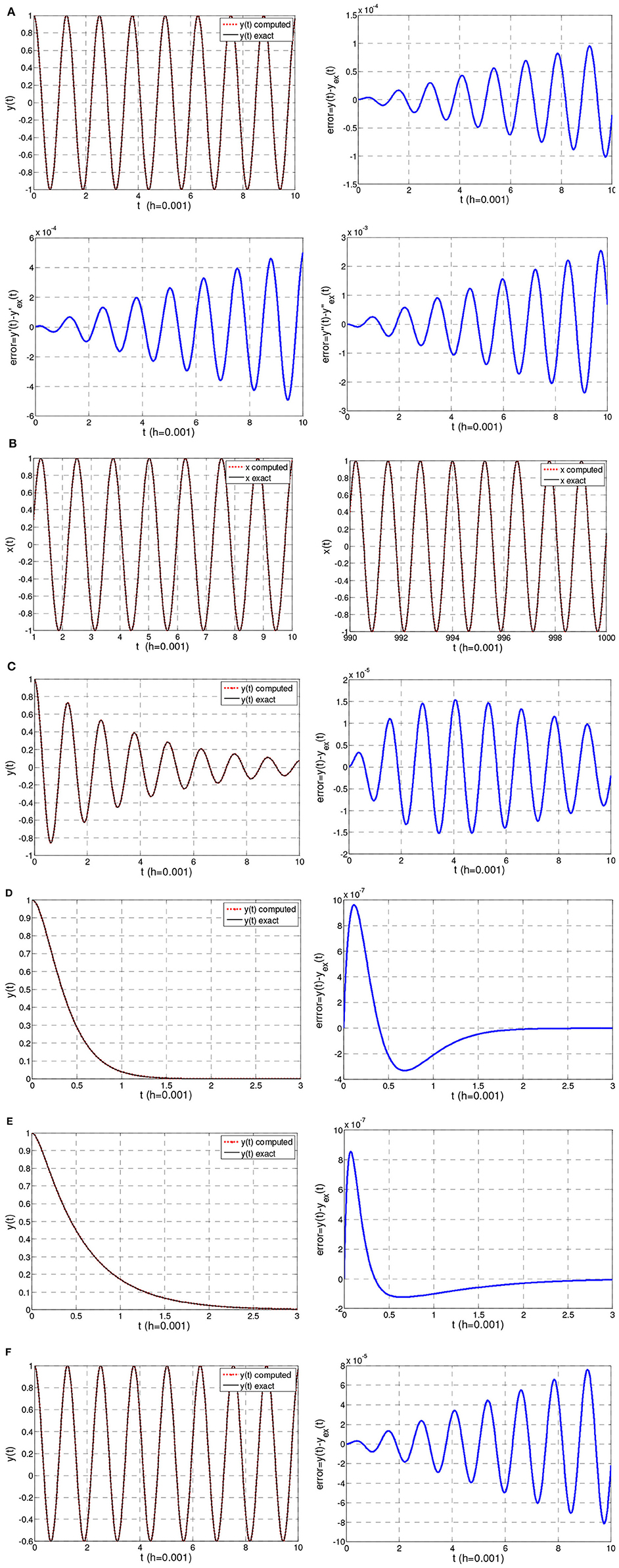
Figure 1. (A) Solution in Example 1, case (i). (B) Response for long duration in Example 1, case (i). (C) Solution in Example 1, case (ii). (D) Solution in Example 1, case (iii). (E) Solution in Example 1, case (vi). (F) Solution in Example 1, case (v).

Case (ii): a₁ = 0.5, a₂ = 25, f(t) = 0 $y_{0} = 1, y_{0}^{'} = 0$

In this case, Equation (2.22a) represents free underdamped vibrations of a system with one-degree-of-freedom. The problem admits an exact solution (Katsikadelis, 2020)

\begin{array}{l} y (t) = [\frac{y_{0}^{'} + y_{0} ξ ω}{ω_{D}} sin ω_{D} t + y_{0} cos ω_{D} t] e^{- ξ ω t} & (2.24) \end{array}

where $ω_{D} = ω \sqrt{1 - ξ^{2}}$ , ξ = a₁/2ω < 1, $ω = \sqrt{a_{2}}$ . The obtained solution together with the error e = y−y_ex is shown in Figure 1C. The motion is oscillatory.

Case (iii): a₁ = 10, a₂ = 25, f(t) = 0 $y_{0} = 1, y_{0}^{'} = 0$

In this case, it is ξ = a₁/2ω = 1, and Equation (2.22a) represents the motion of an one-degree-of-freedom system with critical damping. The problem admits an exact solution (Katsikadelis, 2020)

\begin{array}{l} y (t) = [y_{0} + (y_{0} ω + y_{0}^{'}) t] e^{- ω t}, ω = \sqrt{a_{2}} & (2.25) \end{array}

The obtained solution together with the error e = y−y_ex is shown in Figure 1D. The motion is non-oscillatory.

Case (iv): a₁ = 15, a₂ = 25, f(t) = 0 y₀ = 1, y₀ = 0

In this case, it is ξ = a₁/2ω = 1.5, and Equation (2.22a) represents the free motion of an overdamped one-degree-of-freedom system. The problem admits an exact solution (Katsikadelis, 2020).

\begin{array}{l} y (t) = (y_{0} cosh Ω t + \frac{y_{0}^{'} + y_{0} ξ ω}{Ω} sinh Ω t) e^{- ξ ω t}, \\ Ω = ω \sqrt{ξ^{2} - 1}, \\ ω = \sqrt{a_{2}} & (2.26) \end{array}

The obtained solution together with the error e = y − y_ex is shown in Figure 1E. The motion is non-oscillatory.

Case (v): a₁ = 0, a₂ = 25, f(t) = f₀H(t) $y_{0} = 1, y_{0}^{'} = 0$ (f₀ = 5)

where H(t) is the Heaviside step function. In this case, Equation (2.22a) represents the forced undamped vibrations of an one-degree-of-freedom system subjected to a suddenly applied load f₀ at t = 0. The problem admits an exact solution (Katsikadelis, 2020).

\begin{array}{l} y (t) = \frac{y_{0}^{'}}{ω} sin ω t + y_{0} cos ω t + \frac{f_{0}}{a_{2}} (1 - cos ω t), \\ ω = \sqrt{a_{2}} & (2.27) \end{array}

Figure 1F shows the obtained solution together with the error e = y − y_exact.

Example 2. Second-Order ODE. Three-Degree-of-Freedom System

In this example, we solve the IVP:

\begin{array}{l} {\begin{matrix} y_{1}^{″} \\ y_{2}^{″} \\ y_{3}^{″} \end{matrix}} + [\begin{matrix} 2.0090 & 0.6166 & 2.0863 \\ 0.3798 & 0.9195 & 0.2483 \\ 1.1996 & 1.1998 & 4.5136 \end{matrix}] {\begin{matrix} y_{1}^{'} \\ y_{2}^{'} \\ y_{3}^{'} \end{matrix}} \\ + [\begin{matrix} 9.4479 & 3.3772 & 1.1120 \\ 4.9086 & 9.0005 & 7.8025 \\ 4.8925 & 3.6925 & 3.8974 \end{matrix}] {\begin{matrix} y_{1} \\ y_{2} \\ y_{3} \end{matrix}} = {\begin{matrix} f_{1} (t) \\ f_{2} (t) \\ f_{3} (t) \end{matrix}} & (2.28a) \end{array}

\begin{array}{l} y_{0} = {\begin{matrix} 1 & 0 & 0 \end{matrix}}^{T}, {y^{'}}_{0} = {\begin{matrix} 0 & 2 & 0.2 \end{matrix}}^{T} & (2.28b) \end{array}

The matrix K, [see Equation (2.4b)] and its eigenvalues are:

\begin{array}{l} K = {[\begin{matrix} 0 & - I \\ a_{3} & a_{2} \end{matrix}]}_{6 \times 6}, & (2.29a) \end{array}

\begin{array}{l} e i g (K) = {\begin{matrix} λ_{1} \\ λ_{2} \\ λ_{3} \\ λ_{4} \\ λ_{5} \\ λ_{6} \end{matrix}} = {\begin{matrix} 3.0431 + 0.0000 i \\ 1.2844 + 2.9891 i \\ 1.2844 - 2.9891 i \\ 0.6193 + 2.1419 i \\ 0.6193 - 2.1419 i \\ 0.5915 + 0.0000 i \end{matrix}} & (2.29b) \end{array}

We observe that Re(λ_i) > 0. Hence, the stability criterion is satisfied and the proposed method can be applied.

Equation (2.28a) for

\begin{array}{l} {\begin{matrix} f_{1} (t) \\ f_{2} (t) \\ f_{3} (t) \end{matrix}} = {\begin{matrix} 0.2224 t + 9.6811 cos t + 4.7454 sin t + 0.41726 \\ 1.5605 t + 6.7476 cos t + 15.6212 sin t + 0.04966 \\ 0.77948 t + 7.2921 cos t + 6.1854 sin t + 0.90272 \end{matrix}} & (2.30) \end{array}

admits the exact solution $y_{e x} = {cos (t) 2 sin (t) t / 5}^{T}$ . Figure 2 shows the solution as compared with the exact one as well as the error e = y − y_ex.

FIGURE 2

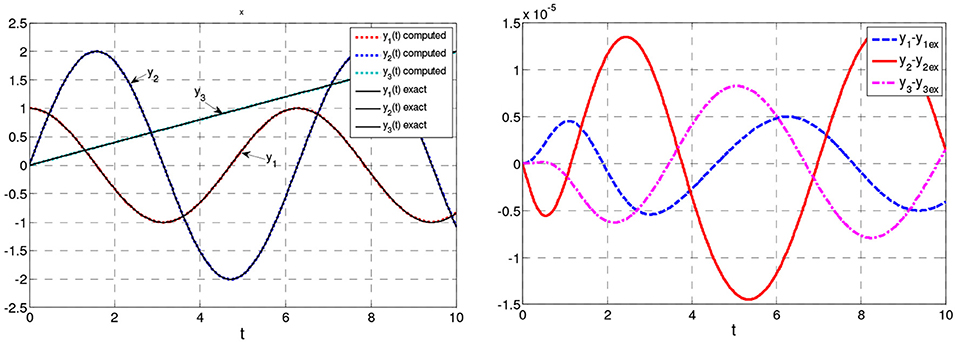
Figure 2. Solution and error in Example 2.

Example 3. Third-Order ODE. Two-Degree-of Freedom System

In this example, we solve the third-order IVP:

\begin{array}{l} {\begin{matrix} y_{1}^{‴} \\ y_{2}^{‴} \end{matrix}} + [\begin{matrix} 4.0735 & 0.6350 \\ 4.5290 & 4.5670 \end{matrix}] {\begin{matrix} y_{1}^{″} \\ y_{2}^{″} \end{matrix}} + [\begin{matrix} 0.6323 & 0.2784 \\ 0.09754 & 0.5468 \end{matrix}] {\begin{matrix} y_{1}^{'} \\ y_{2}^{'} \end{matrix}} \\ + [\begin{matrix} 0.9575 & 0.1576 \\ 0.9649 & 0.9706 \end{matrix}] {\begin{matrix} y_{1} \\ y_{2} \end{matrix}} = {\begin{matrix} f_{1} \\ f_{2} \end{matrix}} & (2.31a) \end{array}

\begin{array}{l} y_{0} = {\begin{matrix} 0 & 2 \end{matrix}}^{T}, y_{0}^{'} = {\begin{matrix} 1 & - 1 \end{matrix}}^{T}, y_{0}^{″} = {\begin{matrix} - 1 & - 1.5 \end{matrix}}^{T} & (2.31b) \end{array}

The matrix K and its eigenvalues are:

\begin{array}{l} K = {[\begin{matrix} 0 & - I & 0 \\ 0 & 0 & - I \\ a_{3} & a_{2} & a_{1} \end{matrix}]}_{6 \times 6}, & (2.32a) \end{array}

\begin{array}{l} e i g (K) = {\begin{matrix} λ_{1} \\ λ_{2} \\ λ_{3} \\ λ_{4} \\ λ_{5} \\ λ_{6} \end{matrix}} = {\begin{matrix} 5.9076 + 0.0000 i \\ 2.6155 + 0.0000 i \\ 0.0209 + 0.5037 i \\ 0.0209 - 0.5037 i \\ 0.0378 + 0.4432 i \\ 0.0378 - 0.4432 i \end{matrix}} & (2.32b) \end{array}

We observe that Re(λ_i) > 0. Hence, the stability criterion is satisfied, and the proposed method can be applied.

Equation (2.31a) for

\begin{array}{l} f = e^{- 0.5 t} [\begin{matrix} - 4.6069 cos t - 1.3023 sin t / 4 \\ 30.2989 sin t / 5 - 178.439 cos t / 25 \end{matrix}] & (2.33) \end{array}

admits an exact solution:

\begin{array}{l} y_{e x} = e^{- 0.5 t} {\begin{matrix} sin t \\ cos t \end{matrix}} & (2.34) \end{array}

Figure 3A shows the computed solution for h = 0.01 as compared with the exact one. Figure 3B shows the error of the solution and its derivatives for h = 0.01. Moreover, Figure 3C shows the error max |y_k(t_i) − (y_ex)_k(t_i)|, (k = 1, 2, 0 < t_i ≤ 100) vs. the time step h. Apparently, this validates the convergence of the numerical scheme. Finally, Figure 3D verifies that the convergence is of O(h²) (Katsikadelis, 2016b).

FIGURE 3

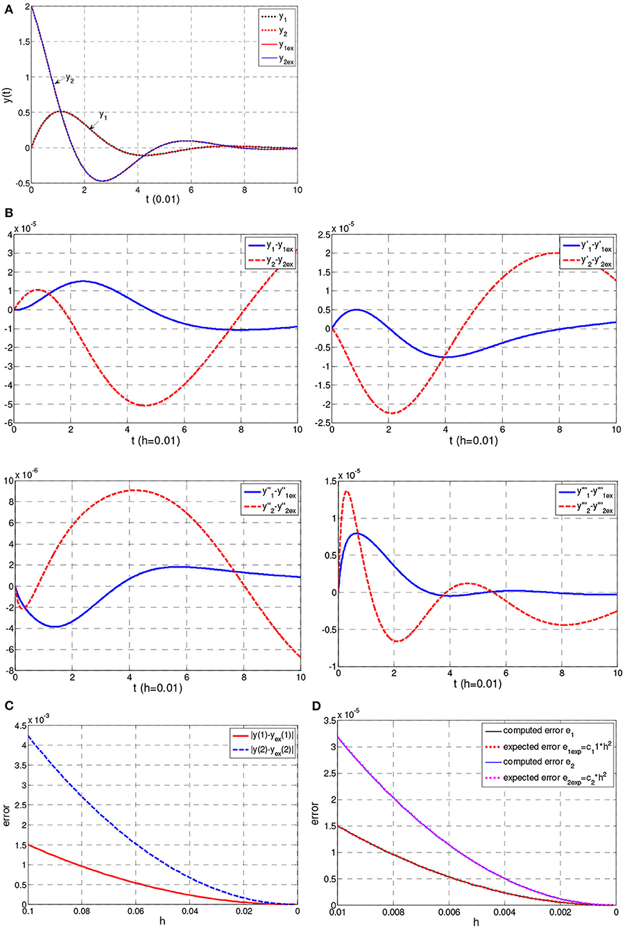
Figure 3. (A) Solution $y = {\begin{matrix} y_{1} & y_{2} \end{matrix}}^{T}$ in Example 3. (B) Error in Example 3. (C) Error max |y_k(t_i) − (y_ex)_k(t_i)| (k = 1, 2, 0 < t_i ≤ 100) in Example 3. (D) Computed and expected error e_k = e_k(h); $c_{k} = e_{k} (1) / h {(1)}^{2}$ (k = 1, 2) in Example 3.

Example 4. Third-Order ODE. One-Degree-of-Freedom System. Stable Solution

In this example, we study the IVP:

\begin{array}{l} y^{‴} + 2 y^{″} + 10 y^{'} + y = 0 & (2.35a) \end{array}

\begin{array}{l} y (0) = 1, y^{'} (0) = - 1, y^{″} (0) = 1 & (2.35b) \end{array}

Equation (2.35a) admits an exact solution:

\begin{array}{l} y_{e x} = c_{1} exp (r_{1} t) + c_{2} exp (r_{2} t) + c_{3} exp (r_{3} t) \end{array}

where,

\begin{array}{l} {\begin{matrix} r_{1} \\ r_{2} \\ r_{3} \end{matrix}} = {\begin{matrix} - 0.9490 + 2.9843 i \\ - 0.9490 - 2.9843 i \\ - 0.1020 + 0.0000 i \end{matrix}}, \\ {\begin{matrix} c_{1} \\ c_{2} \\ c_{3} \end{matrix}} = {\begin{matrix} 0.0371 + 0.1399 i \\ 0.0371 - 0.1399 i \\ 0.9257 - 0.0000 i \end{matrix}} \end{array}

The matrix K and its eigenvalues are:

\begin{array}{l} K = {[\begin{matrix} 0 & - 1 & 0 \\ 0 & 0 & - 1 \\ 1 & 10 & 2 \end{matrix}]}_{3 \times 3} & (2.36a) \end{array}

\begin{array}{l} eig (K) = {\begin{matrix} λ_{1} \\ λ_{2} \\ λ_{3} \end{matrix}} = {\begin{matrix} 0.1020 + 0.0000 i \\ 0.9490 + 2.9843 i \\ 0.9490 - 2.9843 i \end{matrix}} & (2.36b) \end{array}

Obviously, it is Re(λ_i) > 0. Therefore, the solution is stable as it satisfies the stability condition. Figure 4 shows the solution and the corresponding error.

FIGURE 4

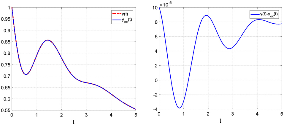
Figure 4. Solution and error in Example 4.

Example 5. Third-Order ODE. One-Degree-of-Freedom System. Unstable Solution

In this example, we study the IVP:

\begin{array}{l} y^{‴} + 2 y^{″} + 10 y^{'} + 25 y = 0 & (2.37a) \end{array}

\begin{array}{l} y (0) = 1, y^{'} (0) = - 1, y^{″} (0) = 1 & (2.37b) \end{array}

Equation (2.37a) admits an exact solution:

\begin{array}{l} y_{e x} = c_{1} exp (r_{1} t) + c_{2} exp (r_{2} t) + c_{3} exp (r_{3} t) \end{array}

where

\begin{array}{l} {\begin{matrix} r_{1} \\ r_{2} \\ r_{3} \end{matrix}} = {\begin{matrix} 0.1623 + 3.2754 i \\ 0.1623 - 3.2754 i \\ - 2.3246 + 0.0000 i \end{matrix}}, \\ {\begin{matrix} c_{1} \\ c_{2} \\ c_{3} \end{matrix}} = {\begin{matrix} 0.1429 + 0.0937 i \\ 0.1429 - 0.0937 i \\ 0.7142 - 0.0000 i \end{matrix}} \end{array}

The matrix K and its eigenvalues are:

\begin{array}{l} K = {[\begin{matrix} 0 & - 1 & 0 \\ 0 & 0 & - 1 \\ 25 & 10 & 2 \end{matrix}]}_{3 \times 3}, & (2.38a) \end{array}

\begin{array}{l} e i g (K) = {\begin{matrix} λ_{1} \\ λ_{2} \\ λ_{3} \end{matrix}} = {\begin{matrix} 5.0000 + 0.0000 i \\ - 1.5000 + 4.7697 i \\ - 1.5000 - 4.7697 i \end{matrix}} & (2.38b) \end{array}

Obviously, it is Re(λ₂) < 0, Re(λ₃) < 0. Therefore, the solution is unstable because it does not satisfy the stability condition. Figure 5 shows the solution and the corresponding error.

FIGURE 5

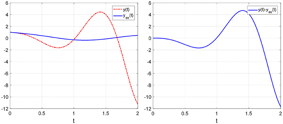
Figure 5. Solution and error in Example 5.

3. Linear Equation With Variable Coefficients

To this point, we have developed the method for the solution of Equation (1.1a) with constant coefficients matrices. If the matrices a₁, a₂, … a_n depend on the variablet, i.e., a₁(t), a₂(t), … a_n(t), the solution procedure described previously remains the same except that the elements in the last row of K, Equation (2.4b) depend on time. Therefore, this matrix must be reevaluated in each time step of the solution procedure. In the following, the efficiency of the method is demonstrated by solving ODEs with variable coefficients.

Example 6. Variable Coefficients. Second-Order ODE. One-Degree-of-Freedom System

In this example, we solve the IVP:

\begin{array}{l} (1 + t^{2}) y^{″} + t y^{'} + e^{1 / (1 + t)} y = p (t) & (3.1a) \end{array}

\begin{array}{l} y_{0} = 1, y_{0}^{'} = - 0.1 & (3.2b) \end{array}

This problem for

\begin{array}{l} p (t) = e^{(- t / 10)} {[e^{1 / (t + 1)} - \frac{99}{100} (t^{2} + 1) - \frac{t}{10}] cos t \\ + (1 - \frac{sin t}{5}) sin t} \end{array}

admits an exact solution $y_{e x} (t) = e^{- 0.1 t} cos (t)$ .

We observe that $a_{1} = \frac{t}{1 + t^{2}} \geq 0$ , $a_{2} = \frac{e^{1 / (1 + t)}}{1 + t^{2}} > 0$ . Therefore, the stability condition is satisfied for all values of t, and the developed solution procedure can be employed. The computed solution in the interval 0 ≤ t ≤ 20 is shown in Figure 6 as compared with the exact one together with the error e = y − y_ex.

FIGURE 6

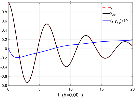
Figure 6. Solution y and error y − y_ex in Example 6.

4. Non-Linear Equations

The n-th Order Non-linear ODE

The solution procedure developed for the linear equations can be straightforwardly extended to non-linear equations. However, in this case, the stability condition applies locally, which demands adequate reduction of the time step to ensure linearization.

The IVP for the non-linear N-degree of freedom systems can be formally stated as:

\begin{array}{l} y^{(n)} + G (t, y, y^{'}, y^{″}, \dots y^{(n - 1)}, y^{(n - 1)}) = f (t), \\ t \in [0, T], T > 0 & (4.1a) \end{array}

\begin{array}{l} y (0) = y_{0}, y^{'} (0) = {y^{'}}_{0}, y^{″} (0) = {y^{″}}_{0}, \dots, y^{(n - 1)} (0) \\ = y_{0}^{(n - 1)} & (4.1b) \end{array}

where G(t, y, y′, y″, … y⁽ⁿ⁻¹⁾, y⁽ⁿ⁻¹⁾) is an N × 1 vector whose elements are in general non-linear functions of the components of the vectors: y, y′, y″, … y⁽ⁿ⁻¹⁾, y⁽ⁿ⁻¹⁾.

Using the transformation (2.1), Equation (4.1a) becomes:

\begin{array}{l} {\begin{matrix} {x^{'}}_{1} \\ {x^{'}}_{2} \\ {x^{'}}_{3} \\ ⋮ \\ {x^{'}}_{n - 1} \\ {x^{'}}_{n} \end{matrix}} + {\begin{matrix} - x_{2} \\ - x_{3} \\ - x_{4} \\ ⋮ \\ - x_{n} \\ G (t, x_{1}, x_{2}, \dots x_{n},) \end{matrix}} = {\begin{matrix} 0 \\ 0 \\ 0 \\ ⋮ \\ 0 \\ f \end{matrix}} & (4.2) \end{array}

Thus, the IVP (4.1a,b) is written in matrix form:

\begin{array}{l} \dot{u} + F (u) = p (t) & (4.3a) \end{array}

\begin{array}{l} u (0) = u_{0} & (4.3b) \end{array}

where

\begin{array}{l} u = {\begin{matrix} x_{1} \\ x_{2} \\ x_{3} \\ ⋮ \\ x_{n - 1} \\ x_{n} \end{matrix}}_{L \times 1}, & (4.4a) \end{array}

\begin{array}{l} F (u) = {\begin{matrix} - x_{2} \\ - x_{3} \\ - x_{4} \\ ⋮ \\ - x_{n} \\ G (t, x_{1}, x_{2}, \dots x_{n},) \end{matrix}}_{L \times 1}, p = {\begin{matrix} 0 \\ 0 \\ 0 \\ ⋮ \\ 0 \\ f \end{matrix}}_{L \times 1} & (4.4b,c) \end{array}

Equation (4.3) is solved using the procedure developed in Katsikadelis (2016b) for the non-linear parabolic equation. Thus, Equation (4.3a) for t = 0 gives:

\begin{array}{l} q_{0} = [p_{0} - F (u_{0})] & (4.5) \end{array}

in which the vector q₀ denotes $\dot{u}$

Then, Equation (4.3a) is applied for t = t_n:

\begin{array}{l} q_{n} + F (u_{n}) = p_{n} & (4.6) \end{array}

Moreover, we have [see (Katsikadelis, 2016b)]:

\begin{array}{l} u_{n} = u_{n - 1} + \frac{h}{2} q_{n - 1} + \frac{h}{2} q_{n} & (4.7) \end{array}

Eqations (4.6) and (4.7) are combined and solved for q_n, u_n with n = 1, 2, … . The solution can be obtained using an iterative procedure in each step. A simple procedure is to substitute Equation (4.7) into Equation (4.6) and solve the resulting non-linear algebraic equation for q_n. The solution can be obtained by employing any ready-to-use subroutine for non-linear algebraic equations. In our examples, the MATLAB function fsolve has been employed to obtain the numerical results. The efficiency of the described procedure to solve non-linear equations is demonstrated by the following examples. All equations satisfy the stability condition locally.

Example 7. Non-linear Second-Order ODE. One-Degree-of-Freedom System

The described numerical procedure is used to solve the IVP for the Duffing equation:

\begin{array}{l} y^{″} + 0.2 y^{'} + y + y^{3} = f (t) & (4.8a) \end{array}

\begin{array}{l} y (0) = 0, y^{'} (0) = 1 & (4.8b) \end{array}

For f(t) = e^−3t(sin t)³/10 − e^−t/10 sin t/100, the IVP (4.8a,b) admits an exact solution $u_{e x} (t) = e^{- 0.1 t} sin t$ .

In this case, the vectors involved in Equations (4.3a,b) are:

\begin{array}{l} u = {\begin{matrix} x_{1} \\ x_{2} \end{matrix}}, G (u) = {\begin{matrix} - x_{2} \\ 0.2 x_{2} + x_{1} + x_{1}^{3} \end{matrix}}, \\ p (t) = {\begin{matrix} 0 \\ f (t) \end{matrix}}, u_{0} = {\begin{matrix} 0 \\ 1 \end{matrix}} \end{array}

The solution together with the error y − y_ex for Δt = 0.01 is shown in Figure 7A. Besides, Figure 7B shows the phase plane of the solution.

FIGURE 7

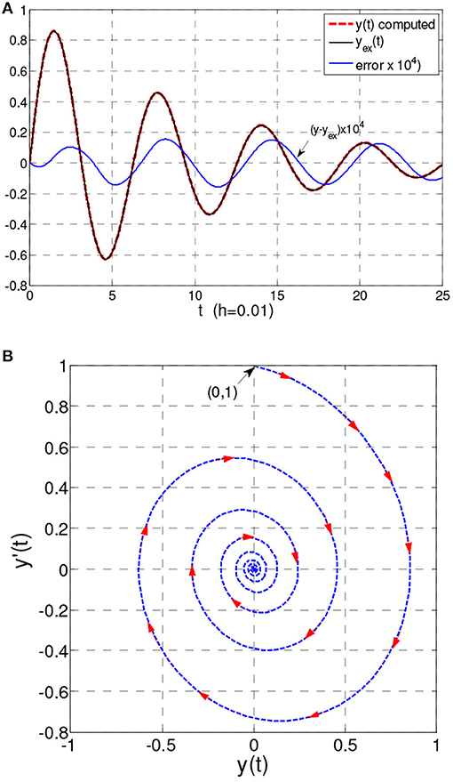
Figure 7. (A) Solution y(t) and error y − y_ex in Example 7. (B) Phase plane (0 ≤ t ≤ 500, h = 0.1) in Example 7.

Example 8. Non-linear Second-Order ODE. One-Degree-of-Freedom System Exhibiting Softening

The numerical procedure for non-linear equations is employed to solve the IVP describing the response of a system exhibiting softening, namely,

\begin{array}{l} y^{″} + 0.2 y^{'} + 40 y - y^{3} = f (t) & (4.9a) \end{array}

\begin{array}{l} y (0) = 0, y^{'} (0) = 1 & (4.9b) \end{array}

For f(t) = 38.99e^−0.1t sin t − e^−0.3t(sin t)³, the IVP (4.9a,b) admits an exact solution $y_{e x} (t) = e^{- 0.1 t} sin t$ .

In this case, the vectors involved in Equations (4.3a,b) are:

\begin{array}{l} u = {\begin{matrix} x_{1} \\ x_{2} \end{matrix}}, G (u) = {\begin{matrix} - x_{2} \\ 0.2 x_{2} + 40 x_{1} - x_{1}^{3} \end{matrix}}, \\ p (t) = {\begin{matrix} 0 \\ f (t) \end{matrix}}, u_{0} = {\begin{matrix} 0 \\ 1 \end{matrix}} \end{array}

The computed solution and its derivative are shown in Figures 8A,B, respectively, as compared with the exact ones. Moreover, the computed error y − y_ex for Δt = 0.01 is shown in Figure 8C. Apparently, the obtained results show that the proposed method can solve efficiently systems exhibiting softening.

FIGURE 8

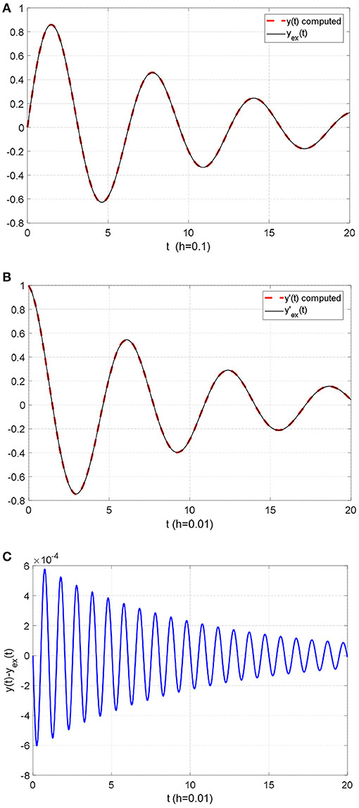
Figure 8. (A) Solution y(t) in Example 8. (B) Derivative y′(t) of the solution in Example 8. (C) Error y − y_ex in Example 8.

Example 9. The Van Der Pol Equation

In this example, the IVP for the Van der Pol equation is solved, namely,

\begin{array}{l} y^{″} + μ (1 - y^{2}) y^{'} + y = 0 & (4.10a) \end{array}

\begin{array}{l} y (0) = 0, y^{'} (0) = 0.1 & (4.10b) \end{array}

The solution obtained for various values of the parameter μ is shown in Figure 9. Apparently, the method works for a long duration and large values of μ, where the system becomes stiff.

FIGURE 9

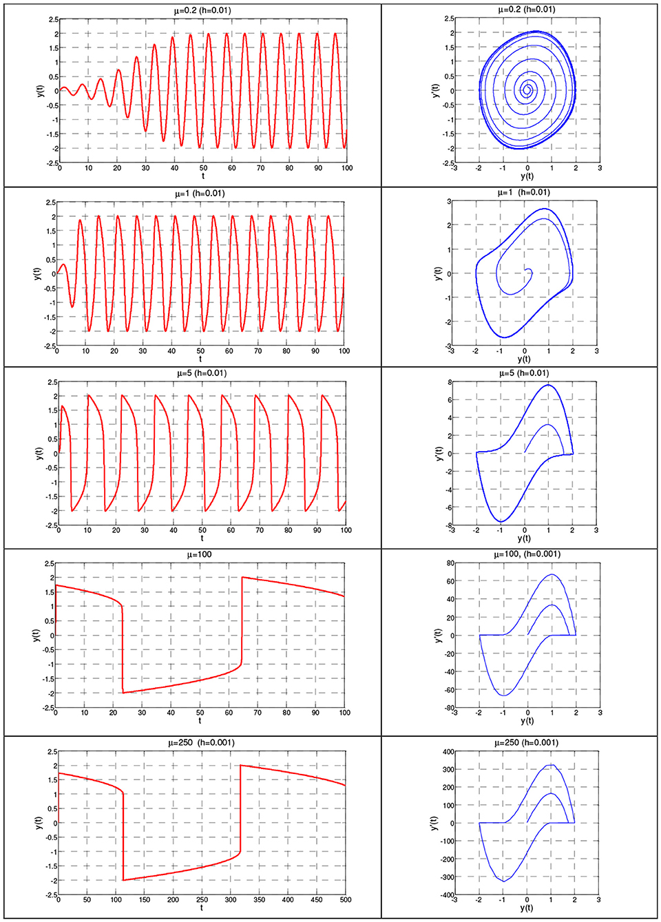
Figure 9. Solution y(t) and phase plane in Example 9.

Example 10. The Elastic Pendulum

The elastic pendulum (Figure 10A) is chosen as a two-degree-of-freedom non-linear system. In this pendulum, the rod is assumed elastically extensible with an axial stiffness k = EA/l, where A is the area of the cross-section of the rod and E the modulus of elasticity of its material.

FIGURE 10

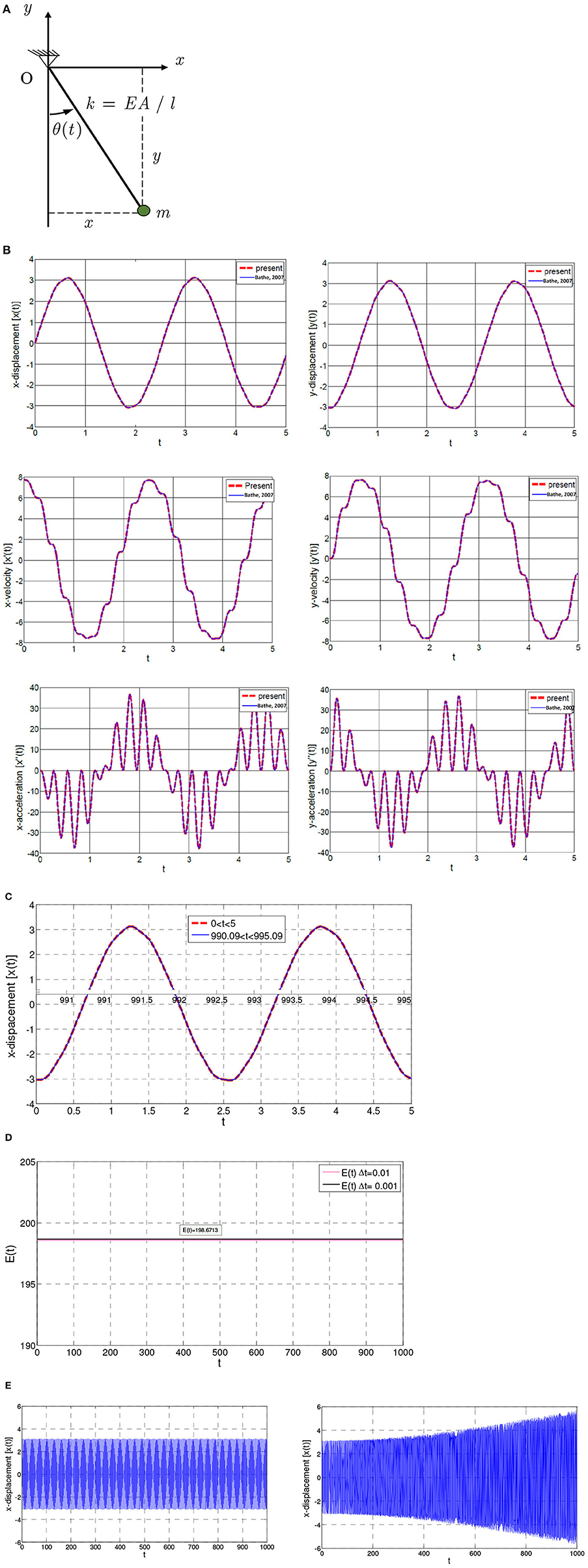
Figure 10. (A) Elastic pendulum in Example 10. (B) Elastic pendulum using the present scheme with Δt = 0.001 in Example 10. (C) The x-displacement in the time intervals 0 < t < 5 and 990.09 < t < 995.09 with Δt = 0.01 in Example 10. (D) Energy variation in Example 10. (E) The x-displacement using (left) current scheme with Δt = 0.01 and (right) Newmark's trapezoidal rule with Δt = 0.00001 in Example 10.

In Cartesian coordinates x(t) y(t), the motion of the pendulum is governed by the two non-linear equations of motion (Katsikadelis, 2020).

\begin{array}{l} m \ddot{x} + \frac{E A}{L} (1 - \frac{L}{\sqrt{x^{2} + y^{2}}}) x = 0 & (4.11a) \end{array}

\begin{array}{l} m \ddot{y} + \frac{E A}{L} (1 - \frac{L}{\sqrt{x^{2} + y^{2}}}) y = - m g & (4.11b) \end{array}

with the initial conditions.

\begin{array}{l} x (0) = x_{0}, \dot{x} (0) = {\dot{x}}_{0}, y (0) = y_{0}, \dot{y} (0) = {\dot{y}}_{0} & (4.12) \end{array}

This problem, in absence of gravity, i.e., mg = 0, has been used as a benchmark problem by earlier investigators (Bathe, 2007) to check the performance of their method in an effort to overcome the instability of the Newmark method arising when long-duration motions are considered in non-linear structural dynamics.

The pendulum is studied using the procedure presented in Section Non-linear Equations with data: l = 3.0443m, EA = 10⁴N, x₀ = 0, $ẋ_{0} = 7.72 {ms}^{- 1},$ y₀ = −l, ẏ₀ = 0, m = 6.667 kg, ρA = 6.57kg/m, which are the data employed in Bathe (2007). The response of the system obtained with Δt = 0.001 is presented in Figure 10B and is identical with the exact solution (Beléndez et al., 2007). In Figure 10C, the x-displacement obtained with Δt = 0.001 in the intervals 0 ≤ t ≤ 5 and 990.09 ≤ t ≤ 995.09 has been plotted. This demonstrates that the response remains unchanged after a long duration of motion. Figure 10D shows that the total energy of the system is conserved. It is apparent that the proposed method does not exhibit a period elongation and an amplitude decay when analyzing the dynamic response of non-linear systems (Kuhl and Crisfield, 1999). Finally, Figure 10E shows the response of the elastic pendulum obtained using the current scheme with Δt = 0.01 and Newmark's trapezoidal scheme with Δt = 0.00001. Apparently, the present scheme performs well for a relatively large time step, while Newmark's scheme shows instability even for a very small time step.

Example 11. Variable Coefficients. Second-Order Non-linear ODEs. Two-Degree-of-Freedom System

The motion of a planet around the Sun is described by the system of differential equations:

\begin{array}{l} \frac{d}{d t} (m_{p} \dot{x}) + G m_{p} M_{S} \frac{x}{r^{3}} = 0 & (4.13a) \end{array}

\begin{array}{l} \frac{d}{d t} (m_{p} \dot{y}) + G m_{p} M_{S} \frac{y}{r^{3}} = 0 & (4.13b) \end{array}

subject to the initial conditions

\begin{array}{l} {x (0), y (0)} = {x_{0}, y_{0}}, \dot{x} (0), ẏ (0)} = {{\dot{x}}_{0}, {\dot{y}}_{0}} & (4.13c,d) \end{array}

where r = (x² + y²)^1/2; m_p, M_S the mass of the planet and Sun, respectively, and G the universal gravitation constant (Murray and Dermott, 1999). For variable planet mass m_p = m₀m(t) and variable Sun mass M_S = M₀M(t), Equations (4.13a,b) are generalized as:

\begin{array}{l} ẍ + \frac{ṁ}{m} ẋ + μ M (t) \frac{x}{r^{3}} = 0 & (4.14a) \end{array}

\begin{array}{l} \ddot{y} + \frac{\dot{m}}{m} \dot{y} + μ M (t) \frac{y}{r^{3}} = 0 & (4.14b) \end{array}

in which μ = GM₀ is the standard gravitational parameter.

Equations (4.14a,b) are solved numerically with μ = 1 and initial conditions:

\begin{array}{l} {x (0), y (0)} = {\begin{matrix} 0 & 13.3333 \end{matrix}}^{T}, \\ {\dot{x} (0), ẏ (0)} = {\begin{matrix} - 0.2738 & 0.09129 \end{matrix}}^{T} & (4.15a,b) \end{array}

First, the solution is obtained for constant Sun mass M(t) = 1, constant planet mass m(t) = 1, and the specified initial conditions (4.15a,b). The exact orbit is the ellipse with r_min = 10 and r_max = 20 (see Figure 11A). Figures 11B,C show the solution as compared with the exact one. Moreover, Figure 11D shows the error = r − r_ex for long the duration of the motion. Note that for h ≤ 0.01, the error does not increase.

FIGURE 11

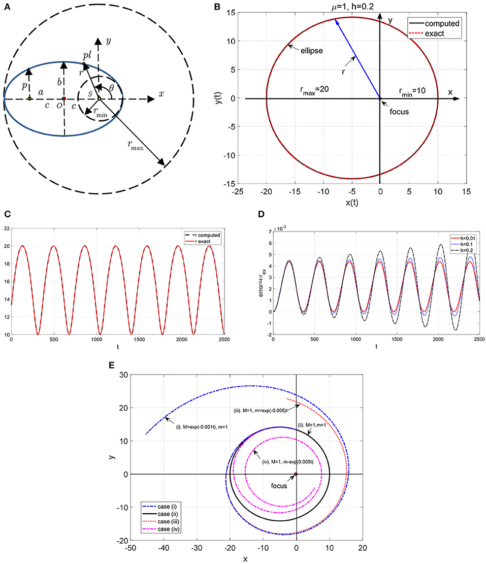
Figure 11. (A) The heliocentric coordinate system (r, θ) for the ellipse in Example 11. (B) Plot of the solution using polar coordinates in Example 11. (C) Plot of the solution r(t) in Example 11. (D) Error = r − r_ex in Example 11. (E) Orbit of a planet when the mass of the planet or the mass of Sun varies with time in Example 11.

The IVP is now solved for a variable mass of the planet and the Sun. Results for the following four cases have been obtained with Δt = 0.2.

(i) Variable Sun mass M(t) = exp(−0.001t) and constant planet mass m(t) = 1.

(ii) Constant Sun mass M(t) = 1 and constant planet mass m(t) = 1.

(iii) Constant Sun mass M(t) = 1 and decreasing planet mass m(t) = exp(−0.005t),

(iv) Constant Sun mass M(t) = 1 and increasing planet mass m(t) = exp(0.005t).

The results have been plotted using polar coordinates in Figure 11E. This figure gives an insight into the behavior of the system Sun-planet when either the mass of the Sun or the mass of the planet varies with time.

Example 12. Fourth-Order ODE. One-Degree-of-Freedom System

In this example, we study the IVP

\begin{array}{l} y^{(i v)} + y^{3} = cos t + {cos}^{3} t & (4.16a) \end{array}

\begin{array}{l} y (0) = 1, y^{'} (0) = 0, y^{″} (0) = - 1, y^{‴} (0) = 0 & (4.16b) \end{array}

The problem admits the exact solution y_ex(t) = cos t.

In this case, the vectors involved in Equations (4.3 a,b) are:

\begin{array}{l} u = {\begin{matrix} x_{1} \\ x_{2} \\ x_{3} \\ x_{4} \end{matrix}}, G (u) = {\begin{matrix} - x_{2} \\ - x_{3} \\ - x_{4} \\ x_{1}^{3} \end{matrix}}, \\ p (t) = {\begin{matrix} 0 \\ 0 \\ 0 \\ cos t + {cos}^{3} t \end{matrix}}, u_{0} = {\begin{matrix} 1 \\ 0 \\ - 1 \\ 0 \end{matrix}} \end{array}

Figure 12A shows the solution with Δt = 0.005 as compared with the exact one. Moreover, Figure 12B shows the computed error y − y_ex for various values of the time step Δt. The local stability requires a very small time step to reduce the error (see Figure 12B).

FIGURE 12

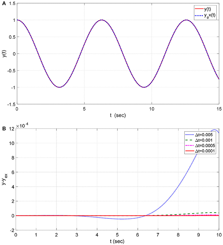
Figure 12. (A) Solution in Example 12 (Δt = 0.005). (B) Error y − y_ex for various values Δtin Example 12.

5. Conclusions

The paper presents a direct time integration method for solving numerically higher-order linear and non-linear ODEs. The quintessence of the method is to use the well-known state-space representation to transform the differential equation of order n > 1 into a system of L = n × N simultaneous first-order equations, and subsequently, to solve it using the numerical method developed recently by Katsikadelis for systems of first-order parabolic differential equations (Katsikadelis, 2016b). An important advantage of the developed method is that it captures the periodic behavior of the solution, where many of the standard numerical methods may be ineffective or produce highly inaccurate results.

The investigation of the stability of the numerical scheme results in the condition that the coefficient matrices of the differential equation must satisfy. The stability does not require symmetrical and positive definite coefficient matrices. This advantage is important because the scheme can find the solution of differential equations resulting from methods in which the space discretization does not result in symmetrical matrices, for example, the boundary element method.

The present method also solves equations having variable coefficients if the stability condition is satisfied in all instances. For non-linear equations, the derived stability condition should be satisfied locally. The method is simply implemented and self-starting. It has second-order accuracy and does not have numerical damping or period elongation. It performs well when motions of long duration are considered, and it can be employed as a practical method for integration of stiff higher-order differential equations as well as equations with stiffness softening, where widely used methods may not be effective. Several well-corroborated examples and numerical experiments are presented, including linear as well as non-linear equations of benchmark problems, which demonstrate the efficiency and accuracy of the developed method.

Data Availability Statement

The raw data supporting the conclusions of this article will be made available by the authors, without undue reservation.

Author Contributions

The author confirms being the sole contributor of this work and has approved it for publication.

Conflict of Interest

The author declares that the research was conducted in the absence of any commercial or financial relationships that could be construed as a potential conflict of interest.

References

Bathe, K. J. (2007). Conserving energy and momentum in non-linear dynamics: a simple implicit time integration scheme. Comput. Struct. 85, 437–445. doi: 10.1016/j.compstruc.2006.09.004

CrossRef Full Text | Google Scholar

Beléndez, A., Pascual, C., Méndez, D. I., Beléndez, T., and Neipp, C. (2007). Exact solution for the non-linear pendulum. Rev Brazil Ensi Fisica 29, 645–648. doi: 10.1590/S1806-11172007000400024

CrossRef Full Text | Google Scholar

Butcher, J. C. (2000). Numerical methods for ordinary differential equations in the 20th century. J. Comp. Appl. Math. 125, 1–29 doi: 10.1016/S0377-0427(00)00455-6

CrossRef Full Text | Google Scholar

Butcher, J. C. (2008). Numerical Methods for Ordinary Differential Equations, second ed., Chichester: John Wiley & Sons Ltd. doi: 10.1002/9780470753767

CrossRef Full Text | Google Scholar

Katsikadelis, J. T. (2014). The Boundary Element Method for Plate Analysis. Oxford: Academic Press, Elsevier.

Google Scholar

Katsikadelis, J. T. (2016a). The Boundary Element Method for Engineers and Scientists. Oxford: Academic Press, Elsevier. doi: 10.1016/B978-0-12-804493-3.00005-9

CrossRef Full Text | Google Scholar

Katsikadelis, J. T. (2016b). A new direct tim integration method for the semi-discrete parabolic equations. Eng. Analy. Bound. Elem. 73, 181–190. doi: 10.1016/j.enganabound.2016.09.009

CrossRef Full Text | Google Scholar

Katsikadelis, J. T. (2020). Dynamic Analysis of Structures. Oxford: Academic Press, Elsevier.

Kuhl, D., and Crisfield, M. A. (1999). Energy-conserving and decaying algorithms. Int. J. Numer. Methods Eng. 45, 569–599. doi: 10.1002/(SICI)1097-0207(19990620)45:5<569::AID-NME595>3.0.CO;2-A

CrossRef Full Text | Google Scholar

Lambert, J. D. (1991). Numerical Methods for Ordinary Differential Systems. The Initial Value Problem. New York, NY: John Wiley & Sons Ltd.

Google Scholar

Murray, C. D., and Dermott, S. F. (1999). Solar System Dynamics. Cambridge: Cambridge University Press. doi: 10.1017/CBO9781139174817

CrossRef Full Text | Google Scholar

Nerantzaki, M. S., and Babouskos, N. G. (2012). Vibrations of inhomogeneous anisotropic viscoelastic bodies described with fractional derivative models. Eng. Analy. Bound. Elem. 36, 1894–1907. doi: 10.1016/j.enganabound.2012.07.003

CrossRef Full Text | Google Scholar

Padhi, S., and Pati, S. (2014). Theory of Third-Order Differential Equations. New Delhi: Springer. doi: 10.1007/978-81-322-1614-8

CrossRef Full Text | Google Scholar

Simos, T. E. (1997). Modifying the Runge-Kutta method for the numerical solution of ODEs with oscillating solutions. Appl. Math. Comp. 84, 131–143. doi: 10.1016/S0096-3003(96)00083-5

CrossRef Full Text | Google Scholar

Keywords: ordinary differential equations, higher-order, numerical method, analog equation method, linear equations, non-linear equations, variable coefficients, boundary element method

Citation: Katsikadelis JT (2021) A New Method for Numerical Integration of Higher-Order Ordinary Differential Equations Without Losing the Periodic Responses. Front. Built Environ. 7:621037. doi: 10.3389/fbuil.2021.621037

Received: 24 October 2020; Accepted: 10 March 2021;
Published: 22 April 2021.

Edited by:

Eleni N. Chatzi, ETH Zürich, Switzerland

Reviewed by:

Dimitrios Lignos, École Polytechnique Fédérale de Lausanne, Switzerland
Aram Soroushian, International Institute of Earthquake Engineering and Seismology, Iran

Copyright © 2021 Katsikadelis. This is an open-access article distributed under the terms of the Creative Commons Attribution License (CC BY). The use, distribution or reproduction in other forums is permitted, provided the original author(s) and the copyright owner(s) are credited and that the original publication in this journal is cited, in accordance with accepted academic practice. No use, distribution or reproduction is permitted which does not comply with these terms.

*Correspondence: John T. Katsikadelis, jkats@central.ntua.gr

ORIGINAL RESEARCH article

A New Method for Numerical Integration of Higher-Order Ordinary Differential Equations Without Losing the Periodic Responses

1. Introduction

2. Linear Equations

The n-th Order Linear ODE

Stability of the Numerical Scheme

Proof

Numerical Examples

Example 1. Second-Order ODE. One-Degree-of-Freedom System

Example 2. Second-Order ODE. Three-Degree-of-Freedom System

Example 3. Third-Order ODE. Two-Degree-of Freedom System

Example 4. Third-Order ODE. One-Degree-of-Freedom System. Stable Solution

Example 5. Third-Order ODE. One-Degree-of-Freedom System. Unstable Solution

3. Linear Equation With Variable Coefficients

Example 6. Variable Coefficients. Second-Order ODE. One-Degree-of-Freedom System

4. Non-Linear Equations

The n-th Order Non-linear ODE

Example 7. Non-linear Second-Order ODE. One-Degree-of-Freedom System

Example 8. Non-linear Second-Order ODE. One-Degree-of-Freedom System Exhibiting Softening

Example 9. The Van Der Pol Equation

Example 10. The Elastic Pendulum

Example 11. Variable Coefficients. Second-Order Non-linear ODEs. Two-Degree-of-Freedom System

Example 12. Fourth-Order ODE. One-Degree-of-Freedom System

5. Conclusions

Data Availability Statement

Author Contributions

Conflict of Interest

References

People also looked at