Serial monitoring of the audiogram in hearing conservation using Gaussian processes

1 Introduction

Audiometric serial monitoring is the act of evaluating changes in hearing thresholds. Audiologists identify changes in a patient's hearing by comparing audiogram results over time. The rationale is that pure tone sensitivity, as measured by the audiogram, is susceptible to damage from audiopathic exposures such as noise or ototoxic medications, and reflect changes associated with normal aging and certain disease conditions. A change in pure-tone sensitivity is taken as evidence of potential audiopathic injury, motivating follow-up care and/or removal from the audiopathic exposure.

There are many serial monitoring criteria described in the audiology literature (reviews in King and Brewer, 2018 and Moore et al., 2022). There are three particular difficulties with all existing approaches:

1) Lack of a gold standard: since there is no gold standard for audiopathic injury and thus no way to evaluate the accuracy of these various criteria, it is up to the clinician or employer to choose among serial monitoring criteria based on clinical objectives, convention, intuition, invasiveness, time, expense, or any other priority. Priorities differ among the end users such as the audiologist, primary care clinician, employer, and patient. The various monitoring criteria can not simultaneously achieve the objectives of all stakeholders resulting in inefficient care.

2) Bias due to no response: the audiologist must also decide how to handle thresholds that exceed audiometer test limits, called “No Response” (NR), or how to handle missing thresholds due to patient non-response. The latter is particularly challenging in pediatric applications, while the former often occurs in older populations of patients. How NR and missing thresholds are handled will impact clinical judgements.

3) Bias due to regression to the mean: regression to the mean is the (almost) ineluctable fact that, barring any real changes, bigger than average baselines are always expected to get smaller and that smaller than average baselines are always expected to get bigger. This is necessarily true in (almost) any homeostatic system, real or imaginary. The previous parenthetical statements invoke certain technical points that can be studied in Samuels (1991). In the absence of audiopathic injury, regression to the mean (Royston, 1995) guarantees that on average a “large” or “high” baseline threshold will be followed by a “smaller” or “lower” one, and that a “small” baseline threshold will be followed by a “larger” one. This is expected regardless of any audiopathic injury that may have occurred. This clearly confounds any attempt to judge audiometric changes in terms of potential injury to the patient, because any observed changes are at least partially due to regression to the mean. A proper approach is to statistically condition the expected follow-up measurement on the previously observed baseline (Royston, 1995). The clinical expectation about a patient at follow-up naturally depends on what was observed at baseline, and a proper statistical expectation for a patient at follow-up must also depend on the previously observed baseline. Regression to the mean induces bias in all existing serial monitoring criteria (Royston, 1995).

Point (1) impacts most every facet of audiology or medicine. Points (2) and (3) occur in most hearing monitoring criteria because standard methods of evaluating changes in pure tone sensitivity are based on the computed difference between baseline and follow-up audiograms. While intuitive, the computed difference approach will cause bias and loss of information. The audiologist must manually perform the differencing computations to determine if a given criterion has been met. Subsequently, the audiologist must communicate the results to the patient and other stakeholders in their care (family, care team). There is a need for rapid or even real-time communication of these results, particularly when results indicate the need for care coordination, for example to eliminate or reduce the audiopathic exposure, or promote timely access to treatment. An unbiased, rapid and transparent way to communicate serial monitoring results would promote more efficient care.

We propose a different approach in this paper to address points (2) and (3). In our view, serial monitoring occurs under the assumption that pure tone sensitivity does not change between the baseline and follow-up time point. We call this the “Homeostasis Hypothesis,” and audiometric serial monitoring is conducted to evaluate whether or not the Homeostasis Hypothesis is true. In this paper we develop a statistical model of the relationship between the audiogram and a patient's underlying pure tone sensitivity under the assumption that the Homeostasis Hypothesis is true. If the follow-up audiogram is unusual with respect to the expectations of the Homeostasis Hypothesis, then the audiologist has evidence against the assumption that pure tone sensitivity has remained constant over the course of exposure. Follow-up action is therefore warranted.

Figure 1 illustrates our approach as described in this paper. Given the patient's baseline audiogram as an input, we compute the predictive distribution of the follow-up audiogram under the assumption that the Homeostasis Hypothesis is correct. Correlations between thresholds in each ear and at neighboring frequencies, as well as population-based pure-tone threshold data are used to narrow the patient-specific predictive distribution. This predictive distribution is expressed as a simultaneous prediction region, which can be easily interpreted: nine out of 10 follow-up audiograms on the patient will be entirely within the region if the Homeostasis Hypothesis is correct. A follow-up audiogram that exceeds the audiogram prediction region at any frequency in either ear is evidence that the Homeostasis Hypothesis is false and that pure tone sensitivity has changed.

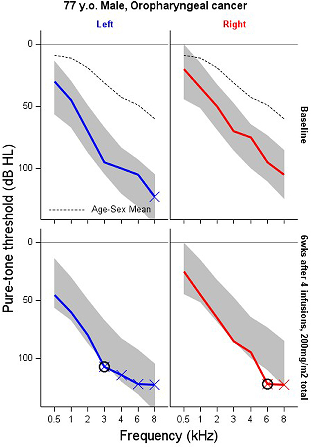
Figure 1. Serial monitoring an adult male, 77 years old, being treated for Oropharyngeal cancer with 40 mg/m², weekly. Solid lines show the pre-treatment baseline audiogram (top row) and 6-week follow-up (bottom row) after four infusions of cisplatin equaling a cumulative dose 200 mg/m². The dashed line is the ISO 1999-2013 (ISO, 2013) age-sex specific mean threshold obtained from population-based pure-tone threshold data. The “X” indicates No Response at that test frequency. The shaded area is a 90% prediction region for this patient's audiogram under the assumption that pure tone sensitivity hasn't changed from their baseline test. Follow-up thresholds exceeding the prediction region (circled) are “significant” changes to the audiogram that warrant follow-up.

In this paper we will take advantage of recent interest in Gaussian Processes in audiology (Song et al., 2015; Bao et al., 2017; Barbour et al., 2019). This methodology provides an alternative to traditional grading or binary scales that are prone to the biases discussed above. This methodology is suitable for patients and employees at risk of audiopathic injury from any type of exposure (e.g., noise, bactericidal or antineoplastic therapies, etc.) as long as baseline audiometry is available. We do not make recommendations about pure tone test frequencies, testing intervals, or procedures for treating patients with audiopathic injury. These decisions are specific to each exposure and are left to the serial monitoring program. Our approach avoids bias and loss of information that affects current approaches, and we believe it can serve a wider range of clinical objectives and stakeholder priorities than standard criteria currently in use. These benefits are achieved at the cost of computational efficiency; i.e., a computer is required, though this burden is small since all computation is automated and done offline. This is an additional benefit of our approach over existing criteria since it maximizes time efficiency and can be administered using computer-based portable audiometry systems at the point of care. The prediction region such as seen in Figure 1 are computed prior to the follow-up exam, and thus do not impinge on patient-audiologist contact time.

2 Methods

The clinical problem for the audiologist is that of deciding whether a follow-up audiogram measured on a patient demonstrates evidence that pure tone sensitivity has degraded and that the Homeostasis Hypothesis is false. The statistical problem is that of defining (1) the relationship between pure tone sensitivity—a theoretical construct that we cannot observe directly—and its representation as the audiogram, and (2) defining the expected relationship between baseline and follow-up audiograms under the assumption that the Homeostasis Hypothesis is correct.

We assume that pure tone sensitivity δ in each ear e and across the frequency spectrum f at baseline time 0 and follow-up time t are Gaussian Processes with covariance functions K₀ and K_t, and population gender- and age-specific mean function μ(e, f ):

This model contains the important assumption that the time that passes between baseline and follow-up measurements (i.e. t) is less than the amount of time that is required before the population age-specific mean function μ(e, f) changes. In other words, the model assumes that monitoring occurs over months, during which time normal presbycusis is effectively unmeasurable, and not decades, when many accumulated factors unrelated to the exposure of concern can induce hearing changes. An expanded model is described in Bao et al. (2017).

The pure tone sensitivity δ(e, f) is measured by the audiogram at test frequencies defined by the clinical protocol. Viewed in this way, the baseline and follow-up audiograms are each an error-susceptible sample from the pure tone sensitivity processes δ₀(e, f) and δ_t(e, f). For our purposes, the audiogram Y is comprised of {Left Ear thresholds at 0.5, 1, 2, 3, 4, 6, 8}, {Right Ear thresholds at 0.5, 1, 2, 3, 4, 6, 8} so that Y has 14 elements. The ordering of ears and frequencies in Y must be consistent for intelligibility. Y₀ and Y_t correspond to audiometry at baseline and follow-up. Moving forward, we use δ₀ and δ_t to represent the functions δ₀(e, f) and δ_t(e, f) evaluated in the ears and pure tone frequencies specified by the testing protocol. The process mean μ is defined the same way.

By virtue of the Gaussian process model, Y₀ and Y_t are multivariate normal random variables with respective means δ₀ and δ_t and residual covariance matrices ∑₀ and ∑_t:

The Homeostasis Hypothesis states that pure tone sensitivity has not changed, i.e. that δ_t=δ₀. An important, but often tacit assumption is that variance components, such as ∑ and K (see below) are assumed constant over the monitoring period, so that any contradiction to the Homeostasis Hypothesis is taken as evidence of audiopathic injury and not to changes model variance components. With these assumptions, the joint distribution of the audiograms at baseline and follow-up time points conditional on δ₀ according to the Homeostasis Hypothesis is

We don't know the baseline pure tone sensitivity δ₀ so we integrate expression (1) with respect to the distribution of δ₀. This gives the unconditional joint distribution of Y_t and Y₀ as

where K is a matrix of evaluations of the covariance function K at the frequencies and ears specified by the testing protocol. The conventional squared exponential covariance model between binary ear indicators (0 = left, 1 = right) e and e^* and log₂ frequencies f and f^* is used for this purpose:

which implies between-ear correlation of $\frac{1}{e^{\alpha }}$ and between-octave correlation of $\frac{1}{e^{\beta }}$. We also assume that ∑ is a diagonal matrix with constant diagonal elements σ². Expression (2) is the multivariate form of the “Linear mixed model” (McCulloch and Searle, 2004).

We can think of two uses of expression (2) in serial monitoring. First, we can compute the distribution of the difference between the baseline and follow-up audiograms as

and then develop prediction regions based on this model. Application of this approach is hampered by missing data or NR at either baseline or follow-up, and regression to the mean is in effect so that unusually large differences are often incorrectly interpreted as evidence of physiological change (Royston, 1995).

Instead, we use the pre-exposure baseline audiogram as an unbiased estimate of pure tone sensitivity in the absence of any audiopathic injury caused by the exposure. Having first observed the baseline audiogram, prior to any exposure, it's natural to think of the follow-up audiogram as a test of stability within the auditory system that generated the baseline audiogram, i.e. the follow-up audiogram is a test that the Homeostasis Hypothesis is correct. This motivates computing the conditional distribution of the follow-up audiogram given the observed baseline under Homeostasis. The multivariate Normal model of Y_t and Y₀ implies that the conditional distribution Y_t|Y₀ is also multivariate Normal with expected value

and covariance

McCulloch and Searle (2004) and Rasmussen and Williams (2005).

The goal is to evaluate whether the follow-up audiogram is consistent with expectations given by the baseline audiogram assuming that the Homeostasis Hypothesis is true. We do this by comparing the follow-up audiogram to the multivariate Normal distribution parameterized by expressions (3) and (4). To facilitate clinical applications, the predictive distribution is typically distilled into one or more prediction intervals. A follow-up threshold that lies outside the prediction interval is unexpected and worthy of further consideration, either by clinical referral or even ignoring the result. This decision is left to the attending audiologist.

Ninety percent pointwise prediction intervals for the follow-up threshold at each frequency are given by expression (3) ± 1.64 times the square root of the diagonal elements of expression (4) (a 95% prediction interval substitutes 1.96 for 1.64 and so forth). The result is a vector of lower and upper 90% prediction limits for each ear and test frequency within which each follow-up threshold is predicted to lie. These 90% pointwise prediction intervals are called “pointwise” because they provide 90% prediction intervals for that specific test ear and frequency “point” only. This distinction is important: A 90% pointwise prediction interval for one ear and test frequency is an interval such that 9 in 10 follow-up thresholds in that ear and test frequency will be within the interval. However, we usually want to monitor multiple frequencies in both ears rather than single frequencies in any one ear. A 90% simultaneous prediction region is one in which 9 in 10 audiograms are completely inside the region. We can't use the pointwise intervals for this purpose because potentially far more than one in 10 follow-ups will yield one or more audiometric thresholds outside the 90% pointwise limits if the Homeostasis Hypothesis is correct. Such a naïve application will yield more false-referrals than expected.

We require a 90% simultaneous prediction region for the entire left and right ear audiogram, and not for each ear and frequency individually. Nine in 10 follow-up audiograms should lie entirely within the prediction region if the Homeostasis Hypothesis is correct. Any frequency in either ear with a threshold outside the interval is cause for concern. We define this prediction region following the “volume tube” methodology outlined in Krivobokova et al. (2010), McMillan and Hanson (2014), and Bao et al. (2017). The idea is to numerically expand the width of all the pointwise prediction intervals until exactly 90% of the predicted audiograms are completely contained within the adjusted intervals in both ears and at each test frequency. Let m_j, l_j, and u_j denote the expected value, upper and lower 90% pointwise prediction limits for the j^th ear-by-frequency combination. We first simulate a large number of audiograms from multivariate Normal parameterized by expressions (3) and (4). A 90% simultaneous prediction region is found by numerically searching for a constant c > 1 that adjusts the lower and upper prediction limits at each frequency by m_j−c(m_j−l_j) and m_j+c(u_j−m_j) so that 90% of the simulated audiograms completely lie within the adjusted intervals at all frequencies in both ears.

2.1 Estimation

The predictive distribution of the follow-up audiogram given its baseline is given by the parameters in expressions (3) and (4) and requires as inputs the age-sex specific population mean audiogram μ, the baseline audiogram y₀ and estimates of σ, φ, α, and β. The population mean thresholds for men and women are taken from ISO 1999-2013 (ISO, 2013). We use these population mean estimates to center the distribution of pure tone sensitivities, though the model allows for considerable variation with respect to the population. Unless there are NR thresholds in the baseline response, the model parameters are easily estimated by maximizing the marginal likelihood in expression (2) (Rasmussen and Williams, 2005). We prefer a Bayesian approach so as to easily propagate uncertainty about the parameter estimates into the predictions. This is done through MCMC evaluation of the joint posterior distribution of the model parameters and using those same MCMC evaluations to compute the predictive distribution of Y_t given Y₀. These predictions are then used in the volume-tube methodology for computing prediction regions for the entire audiogram.

A pure tone threshold that exceeds the audiometer's test limits is called “No Response” (NR) in audiology and more generally called “Right-Censored” at the detection limit d in statistics. This feature is commonly observed in time-to-event data such as patient survivorship in biomedical research or equipment reliability in manufacturing. There are several approaches to handling NR thresholds in hearing research, such as imputing the NR threshold to d plus 5 dB or some other constant. Another approach is to treat the NR measurement as completely missing. Neither of these approaches is appealing because imputation by adding an arbitrary constant implies an observation (the NR limit + 5 dB) that was never made, which implies greater certainty about pure tone thresholds than the audiologist can legitimately claim. This will increase the false-referral rate beyond the nominal levels dictated by the monitoring protocol. Conversely, treating the NR measurement as completely missing isn't a valid approach either, since the audiologist knows that the pure tone threshold exceeds the detection limit d. Thresholds that exceed the audiometer detection limit provide valuable information for making accurate inferences about K and ∑ so that more accurate predictions about the follow-up audiogram can be made.

We approach NR thresholds using censored-data models. Expression (1) represents the likelihood σ, φ, α, and β conditional on δ. Without creating additional notation, the Gaussian Process model for δ(e, f) implies that δ is also a multivariate normal random variable, δ ~ N(μ, K). In the absence of any NR thresholds, we eliminate dependence on δ by marginalizing the likelihood in (1) giving expression (2). However, when there are one or more NR in the audiogram we factor the likelihood into scalar contributions from thresholds that we observe as N(y; δ, σ²) and into scalar contributions from NR thresholds as 1−Φ(d; δ, σ²). This latter expression is one minus the Normal cumulative distribution function evaluated at the audiometer's detection limit d.

There is no closed form integral of this factored likelihood with respect to the distribution of δ (Ertin, 2007) meaning that the simplicity achieved with a complete baseline audiogram is lost. However, we can use MCMC to evaluate the joint distribution of δ and the parameters σ, φ, α, and β conditional on the baseline audiogram. Each of these MCMC evaluations generate a predicted follow-up audiogram according to expressions (3) and (4). The 90% pointwise prediction interval are the 5th and 95th percentiles of the generated predictions at each frequency and ear. The volume tube methodology is applied to these predictive distributions to achieve 90% prediction regions over the entire audiogram. The result is a shaded region (Figures 1, 3–5) that expresses the clinical expectation that 9 in 10 follow-up audiograms will lie completely within the shaded region if the Homeostasis Hypothesis is correct.

The width of the interval can be changed, depending on the clinical application. Chemotherapy monitoring may demand a very low false referral rate so as not to withhold life-saving anti-cancer therapy. Larger apparent changes are admissible before alerting the audiologist to deleterious side effects of the therapy. A 95% reference interval may be preferable in this instance instead of the 90% intervals used throughout this paper. Workplace noise damage monitoring may prefer a higher false-referral rate to avoid financial liability. Smaller threshold changes in the noise exposure context will therefore provoke a response from administrators, so that an 80% reference interval may be preferred. These considerations illustrate the relationship between the consequences of a false-referral and the desired width of the reference interval. If false-referrals provoke little harm, then a narrower interval is acceptable, but if the ramifications of a false-referral are serious, then wider reference intervals are desirable. Our approach provides the user complete control over the nominal false-referral rate.

2.2 Priors

We establish priors on α and β by recalling that the between-ear correlation is $\frac{1}{e^{\alpha }}$ and between-octave correlation is $\frac{1}{e^{\beta }}$. We believe that the between-ear correlation in pure tone sensitivity is likely to be >0.5. We also believe that the between-octave correlation is likely to be >0.5, but we admit much greater uncertainty since this feature may vary widely among patients. These requirements suggest to us that α ~ Half−Normal(0.5²) and β ~ Half−Normal(1²). We also take advantage of the fact that of Y_t, Y₀, and δ₀ are multivariate normal random variables, such that the expected value of the absolute difference over time between any two corresponding elements of Y_t and Y₀ is $\frac{2\sigma }{\sqrt{\pi }}$ and between any two pure tone sensitivities across ears and frequencies on the same person is $\frac{2\phi }{\sqrt{\pi }}$. Average absolute test-retest differences are expected below about 15 dB and average between 5 and 10 dB. This suggests the prior σ ~ Gamma(4, 0.6), which has expected value $\frac{4}{0.6}$ and variance $\frac{4}{{0.6}^2}$. The range of pure tone sensitivities across frequencies is expected to vary markedly among patients, though we expect no more than about 135 dB range among pure tone sensitivities within a patient. We assume the prior φ ~ Gamma(1, 0.025), which is parameterized as for the prior on σ. Summary statistics for each of these priors, as well as the induced priors on the correlations and test-retest differences are shown in Table 1. Prior histograms are shown in Figure 2, along with posterior distributions for the patient shown in Figure 1.

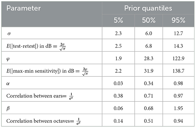
Table 1. Priors on the parameters and the induced parameters of the proposed model.

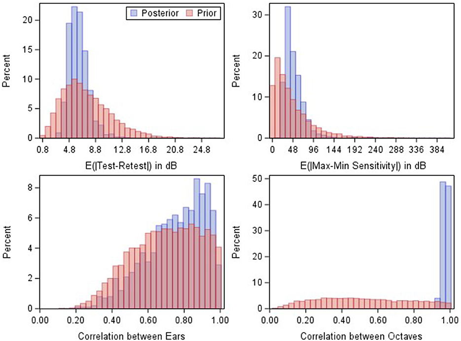
Figure 2. Prior (red) and posterior (blue) MCMC samples for the induced parameters in the model fit to the baseline data shown in Figure 1.

2.3 Computation

The sampler is started at the posterior means from the model in expression (1), initializing NR thresholds at the test limit d. These initial values are fed into a new MCMC sampler replacing expression (2) with expression (1). We find it sufficient to run the MCMC sampler for 500,000 iterations using SAS Enterprise Guide Software, v. 8.3, PROC MCMC, though visual confirmation of efficient mixing is advisable, particularly for unusual audiograms having, for example, elevated left-right asymmetry or many NR thresholds.

3 Results

Figures 3–5 illustrate model results in the context of additional case studies, following the format of Figure 1. The prediction region shown for these patients were generated by inputting the baseline audiogram thresholds, age, and sex into expressions (3) and (4), and following the Volume Tube methodology. Figure 3 shows results for a patient with Cystic Fibrosis who was treated with IV Tobramycin for a bacterial lung infection. Figure 4 shows results for a patient with cancer who was treated with cisplatin, and Figure 5 shows results for an individual exposed to workplace noise over a five-year period. Note that this subject did not provide baseline 3 and 6 kHz thresholds, though the model structure still allows predictions at these frequencies.

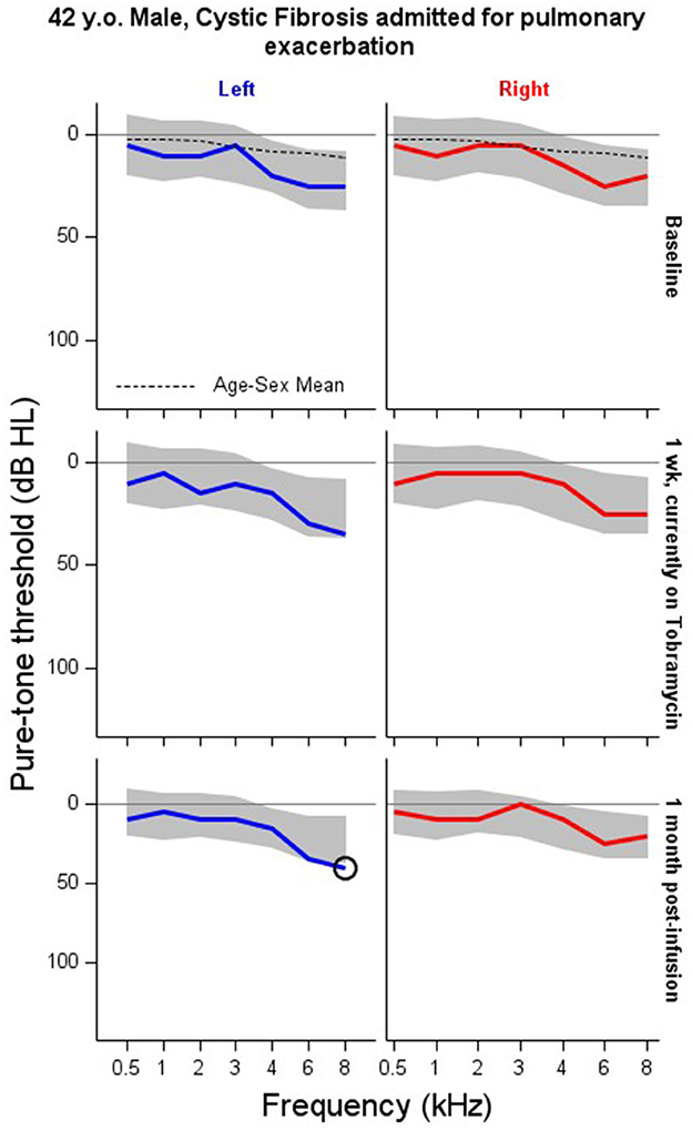
Figure 3. Serial monitoring of a 42 year-old male with a history of pancreatic insufficiency and diabetes mellitus related to his Cystic Fibrosis. The patient presented to emergency unit with a pulmonary infection and was admitted to the hospital where they received between 6.75 to 12.5 ml of IV tobramycin. Visit A: baseline audiogram. Visit B: audiogram taken 1 week after the baseline exam during their course on IV tobramycin therapy as an inpatient. Visit C: first follow-up visit conducted about 1 month after end of IV course of treatment. X = no response, NR. Circled thresholds are significant changes.

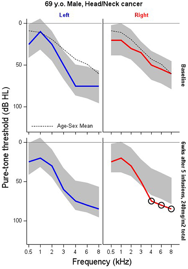
Figure 4. Serial monitoring of a 66 year old patient with a tumor of the suraglottis larynx who received cisplatin-based chemotherapy prior to surgical removal. The patient received five infusions of cisplatin for a total of 240 mg/m². X = no response, NR. Circled thresholds are significant changes.

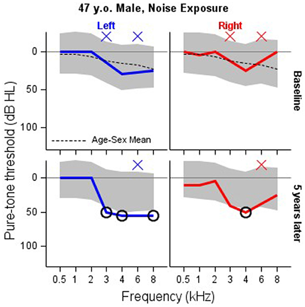
Figure 5. Serial monitoring of a 47 year old patient who worked as a chemical engineer and reported exposure to loud machine noise. His initial audiogram was completed at age 47, with a follow up occurring at age 52. Baseline thresholds are missing at 3 and 6 kHz. 3 kHz thresholds are missing at five-year followup. X = no response, NR. Circled thresholds are significant changes.

4 Discussion

In this paper we describe a Gaussian process regression model of the audiogram that is suitable for serial monitoring in clinical and industrial applications. Additional applications suitably addressed with our approach include monitoring patients for improvements in hearing, for example following surgical intervention such as ossicular reconstruction. The innovative aspects of our approach are three-fold. First, it uses a patient's baseline hearing, known correlations among test frequencies and ears, together with population-based hearing data, to calculate an individualized prediction region for that patient. Second, it provides a unified framework for monitoring the audiogram that is much more intuitive than the various shift criteria commonly used in clinical practice. The automated audiogram region estimated using our approach is simply the region where the follow-up audiogram is predicted to land if that patient's hearing has remained stable. Follow-up thresholds that exceed the predicted region at ANY audiometric frequency can be interpreted as evidence for a statistically significant hearing change. Third, our approach overcomes the problem of regression to the mean, which is a nearly ubiquitous but largely overlooked problem in serial monitoring. The flexibility and ease of interpretation of this model allows for the implementation of the criteria directly into audiometers and other computerized hearing testing platforms, increasing the potential user base and uptake of serial monitoring across contexts.

4.1 Limitations

Our proposal doesn't include any explicit model training commonly used in prediction algorithms. We embed information about the population into the informative priors on the model parameters. An expanded approach is to further train the model in a large sample to identify the joint distribution of model parameters. Training must be done in a population for which the Homeostasis Hypothesis is unequivocally true. Furthermore, this is computationally challenging because of the factored likelihood in the presence of NR thresholds. Training model parameters is the subject of ongoing work by our research group.

Our approach mitigates some of the difficulty of NR thresholds in serial monitoring, though it cannot solve the problem entirely. We can generate prediction regions in the presence of baseline NR, however, any NR observed during follow-up measurements can create difficulties. These are illustrated in Figure 1. The baseline, left-ear, 8 kHz threshold is NR, but our methodology still allows one to identify the prediction region for follow-up thresholds at that frequency and ear. The left-ear, 3 kHz threshold is NR at follow-up, which is outside the expectations established by proposed methodology. In these instances our approach is handling the NR measurement without any trouble as expected. Difficulties arise when the prediction region “straddles” the NR level such as left-ear, 4, 6, and 8 kHz. The observed NR are consistent with the prediction region that spans the test limit, so that no violation of the Homeostasis Hypothesis is observed. However, this isn't exactly true: an NR threshold may actually be outside the prediction region, but the test limit doesn't permit the audiologist to observe this. There is thus some degree of uncertainty one has to accept in these instances.

Although we have developed and described this approach to address the clinical challenge of determining when audiopathic damage has occurred for an adult patient or worker, the framework is easily extended to pediatric applications as long as suitable priors for this population can be identified. This methodology is also easily generalized to “objective measures” of auditory sensitivity that can be obtained reliably in infants and young children. Otoacoustic emissions are an attractive measure to use due to their sensitivity to noise and ototoxic exposures (Dreisbach et al., 2023) and the large literature of test-retest data in unexposed young controls (Bao et al., 2017; Konrad-Martin et al., 2020). Digital audiometry platforms to determine what constitutes a statistically significant hearing change for that patient, will also provide important efficiencies for future clinical trials.

5 Conclusions

Audiogram forecasting such as described in this paper can substantially improve serial monitoring over traditional approaches. Our method avoids sources of bias that reduce diagnostic accuracy and standardizes the definition of a “significant hearing change”. This has the added benefit of leaving clinical interpretations about the functional impacts, implications for follow-up, and treatment options up to the treating audiologist and other clinical stakeholders.

Data availability statement

The raw data supporting the conclusions of this article will be made available by the authors, without undue reservation.

Ethics statement

The studies involving humans were approved by Oregon Health and Science University/VA Portland Joint IRB. The studies were conducted in accordance with the local legislation and institutional requirements. The participants provided their written informed consent to participate in this study.

Author contributions

GM: Conceptualization, Data curation, Formal analysis, Methodology, Software, Visualization, Writing – original draft, Writing – review & editing. JD: Conceptualization, Data curation, Investigation, Methodology, Project administration, Supervision, Visualization, Writing – original draft, Writing – review & editing. MH: Data curation, Investigation, Project administration, Visualization, Writing – review & editing. DK-M: Conceptualization, Formal analysis, Funding acquisition, Investigation, Methodology, Resources, Supervision, Visualization, Writing – original draft, Writing – review & editing.

Funding

The author(s) declare that financial support was received for the research, authorship, and/or publication of this article. This material was the result of work supported with resources and the use of facilities at the VA Rehabilitation Research and Development (RR&D) National Center for Rehabilitative Auditory Research (NCRAR) [Center Award #C2361C/I50 RX002361] at the VA Portland Health Care System in Portland, Oregon and through funding from a VA RR&D Merit Review Award to DK-M [#C3127R/ I01 RX003127].

Acknowledgments

Edward J. Bedrick provided valuable comments that enhanced the manuscript.

Conflict of interest

DK-M is listed as a co-inventor on a patent for a portable hearing test and testing device.

The remaining authors declare that the research was conducted in the absence of any commercial or financial relationships that could be construed as a potential conflict of interest.

Publisher's note

All claims expressed in this article are solely those of the authors and do not necessarily represent those of their affiliated organizations, or those of the publisher, the editors and the reviewers. Any product that may be evaluated in this article, or claim that may be made by its manufacturer, is not guaranteed or endorsed by the publisher.

Author disclaimer

The views expressed in this article are those of the authors and do not necessarily reflect the position or policy of the US Veterans Health Administration or the United States Government.

References

Bao, J., Hanson, T., McMillan, G. P., and Knight, K. (2017). Assessment of DPOAE test-retest difference curves via hierarchical Gaussian processes. Biometrics 73, 334–343. doi: 10.1111/biom.12550
Barbour, D. L., Howard, R. T., Song, X. D., Metzger, N., Sukesan, K. A., DiLorenzo, J. C., et al. (2019). Online machine learning audiometry. Ear Hear. 40, 918–926. doi: 10.1097/AUD.0000000000000669
Dreisbach, L., Konrad-Martin, D., Gagner, C., Reavis, K. M., and Jacobs, P. G. (2023). Descriptive characterization of high-frequency distortion product otoacoustic emission source components in children. J. Speech Lang. Hear. Res. 66, 1–17. doi: 10.1044/2023_JSLHR-23-00013
Ertin, E. (2007). “Gaussian process models for censored sensor readings,” in 2007 IEEE/SP 14th Workshop on Statistical Signal Processing (Madison, WI: IEEE), 665–669. Available online at: http://ieeexplore.ieee.org/document/4301342/ (accessed December 26, 2023).
ISO (2013).14:00–17.00. ISO 1999:2013. Available online at: https://www.iso.org/standard/45103.html (accessed January 8, 2024).
King, K. A., and Brewer, C. C. (2018). Clinical trials, ototoxicity grading scales and the audiologist's role in therapeutic decision making. Int. J. Audiol. 57, S89–S98. doi: 10.1080/14992027.2017.1417644
Konrad-Martin, D., Knight, K., McMillan, G. P., Dreisbach, L. E., Nelson, E., Dille, M., et al. (2020). Long-term variability of distortion-product otoacoustic emissions in infants and children and its relation to pediatric ototoxicity monitoring. Ear Hear. 41:239. doi: 10.1097/AUD.0000000000000536
Krivobokova, T., Kneib, T., and Claeskens, G. (2010). Simultaneous confidence bands for penalized spline estimators. J. Am. Stat. Assoc. 105, 852–863. doi: 10.1198/jasa.2010.tm09165
McCulloch, C. E., and Searle, S. R. (2004). Generalized, Linear, and Mixed Models. Hoboken, NJ: John Wiley and Sons, 358.
McMillan, G. P., and Hanson, T. E. (2014). Sample size requirements for establishing clinical test-retest standards. Ear Hear. 35, 283–286. doi: 10.1097/01.aud.0000438377.15003.6b
Moore, B. C. J., Lowe, D. A., and Cox, G. (2022). Guidelines for diagnosing and quantifying noise-induced hearing loss. Trends Hear. 26:23312165221093156. doi: 10.1177/23312165221093156
Rasmussen, C. E., and Williams, C. K. I. (2005). Gaussian Processes for Machine Learning. Cambridge, MA: MIT Press, 266. doi: 10.7551/mitpress/3206.001.0001
Royston, P. (1995). Calculation of unconditional and conditional reference intervals for foetal size and growth from longitudinal measurements. Stat Med. 14, 1417–1436. doi: 10.1002/sim.4780141303
Samuels, M. L. (1991). Statistical reversion toward the mean: more universal than regression toward the mean. Am. Stat. 45, 344–346. doi: 10.2307/2684474
Keywords: serial monitoring, test-retest, Gaussian process, Bayesian analysis, hearing conservation
Citation: McMillan GP, DeBacker JR, Hungerford M and Konrad-Martin D (2024) Serial monitoring of the audiogram in hearing conservation using Gaussian processes. Front. Audiol. Otol. 2:1389116. doi: 10.3389/fauot.2024.1389116
Received: 21 February 2024; Accepted: 01 April 2024;
Published: 01 May 2024.
Edited by:
Laura Coco, San Diego State University, United StatesReviewed by:
William Bologna, Towson University, United StatesLauren Dillard, Medical University of South Carolina, United States
Copyright © 2024 McMillan, DeBacker, Hungerford and Konrad-Martin. This is an open-access article distributed under the terms of the Creative Commons Attribution License (CC BY). The use, distribution or reproduction in other forums is permitted, provided the original author(s) and the copyright owner(s) are credited and that the original publication in this journal is cited, in accordance with accepted academic practice. No use, distribution or reproduction is permitted which does not comply with these terms.
*Correspondence: J. Riley DeBacker, debacker@ohsu.edu