Bias reduction of maximum likelihood estimation in exponentiated Teissier distribution

Ahmed, Ahmed Abdulhadi; Algamal, Zakariya Yahya; Albalawi, Olayan

doi:10.3389/fams.2024.1351651

ORIGINAL RESEARCH article

Front. Appl. Math. Stat., 20 March 2024
Sec. Statistics and Probability
Volume 10 - 2024 | https://doi.org/10.3389/fams.2024.1351651

Bias reduction of maximum likelihood estimation in exponentiated Teissier distribution

Ahmed Abdulhadi Ahmed¹

Zakariya Yahya Algamal¹^*^†

Olayan Albalawi²^†

¹Department of Statistics and Informatics, University of Mosul, Mosul, Iraq
²Department of Statistics, Faculty of Science, University of Tabuk, Tabuk, Saudi Arabia

The exponentiated Teissier distribution (ETD) offers an alternative for modeling survival data, taking into account flexibility in modeling data with increasing and decreasing hazard rate functions. The most popular method for parameter estimation of the ETD distribution is the maximum likelihood estimation (MLE). The MLE, on the other hand, is notoriously biased for its small sample sizes. We are therefore driven to generate virtually unbiased estimators for ETD parameters. More specifically, we focus on two methods of bias correction, bootstrapping and analytical approaches, to reduce MLE biases to the second order of bias. The performances of these approaches are compared through Monte Carlo simulations and two real-data applications.

1 Introduction

Time-to-event data analysis can be performed statistically using survival data analysis. The time until an event of interest occurs is the main result of interest in survival analysis (1). This could be a number of things, such as the amount of time until a patient relapses, a machine breaks down, or a customer leaves. Statistical modeling of survival data entails modeling and analyzing the amount of time until an event of interest through statistical techniques.

An essential component of survival analysis is selecting a statistical distribution to model survival data (2). The instantaneous failure rate at any given moment is represented by the underlying hazard function, about which different distributions make different assumptions. The properties of the survival data and the underlying biological or physical processes should direct the choice of distribution. Visual evaluations, domain expertise, and goodness-of-fit tests can all be used to guide the selection of a model (3, 4).

In the area of survival analysis, the Teissier distribution is frequently utilized for modeling survival data (5–7). Sharma and Singh (5) presented exponentiated Teissier distributions (ETDs) by adding an extra shape parameter to a well-known baseline distribution. The Teissier distribution is different from other distributions such as Weibull, Gompertz, gamma, and Maxwell distributions in modeling bathtub and upside-down bathtub failure rate functions (5).

The capacity of the Teissier distribution to represent many survival rate phases, such as the growing, constant, and decreasing phases seen in a bathtub failure rate function, is its main advantage. Because it can support many forms and changes in these stages, it is a helpful tool for simulating intricate survival issues.

The Tessier distribution has the following cumulative distribution function (CDF):

\begin{array}{l} F_{T} (z; θ) = 1 - e^{(θ y - e^{θ y} + 1)}; θ > 0, z > 0 & (1) \end{array}

The ETD is defined by CDF:

\begin{array}{l} F_{X} (x; α; θ) = {[F_{T} (x; θ)]}^{α} = {(1 - e^{(θ x - e^{θ x} + 1)})}^{α}; α > 0, θ > 0, x > 0 & (2) \end{array}

The probability density function (PDF) of the ETD is:

\begin{array}{l} f_{X} (x; α; θ) = α θ (e^{θ x} - 1) e^{(θ x - e θ x + 1)} \\ {(1 - e^{(θ x - e θ x + 1)})}^{α - 1}; α > 0, θ > 0, x > 0 \end{array} (3)

2 Maximum likelihood estimation

Suppose that $X = (x_{1}, x_{2}, \dots \dots, x_{n})$ be a random sample of size $n$ from the ETD distribution. The log-likelihood function of $θ$ and $α$ is given by:

\begin{array}{l} L (θ, α) = n + n ln (θ) + n ln (α) - θ \sum_{i = 1}^{n} x_{i} - \sum_{i = 1}^{n} e^{θ x_{i}} + \sum_{i = 1}^{n} ln (e^{θ x_{i}} - 1) \\ + (α - 1) \sum ln (1 - e^{θ x_{i} - e^{θ x_{i}} + 1}) . \end{array} (4)

Maximize Eq. (4) with respect to $θ$ and $α$ in order to obtain the MLE ( $\hat{θ}$ and $\hat{α}$ ) of $θ$ and $α$ _, respectively. We have the following equations:

\begin{array}{l} \frac{\partial}{\partial θ} L (θ, α) = \frac{n}{θ} + \sum_{i = 1}^{n} x_{i} - \sum_{i = 1}^{n} \frac{x_{i} (2 - e^{θ x_{i}})}{1 - e^{θ x_{i}}} \\ + (α - 1) \sum_{i = 1}^{n} \frac{x_{i} (e^{θ x_{i}} - 1)}{e^{- θ x_{i} + e^{θ x_{i}} - 1} - 1} = 0 \end{array} (5)

\begin{array}{l} \frac{\partial}{\partial α} L (θ, α) = \frac{n}{θ} + \sum_{i = 1}^{n} ln (1 - e^{θ x_{i} - e^{θ x_{i}} + 1}) = 0 & (6) \end{array}

Since Eqs. (5) and (6) are non-linear, they cannot be solved analytically. MLE will be biased by small sample sizes. Therefore, it gives misleading results, which affects the interpretation of phenomena in real-life applications. This motivates us to consider unbiased estimates, almost to reduce the bias of this MLE distribution of these parameters.

3 Bias-corrected MLEs

A statistical method called bias-corrected maximum likelihood estimation (BC-MLE) is used to account for bias in parameter estimations that are derived from MLE. When the average value of the estimates, computed across a large number of samples, differs from the true parameter value, the concept of bias in MLE emerges. In order to give more accurate parameter estimates, bias-corrected (BC) approaches try to minimize or completely remove this systematic mistake (8–10).

To evaluate the bias and apply corrections, methods such as the corrective approach (CA) and bootstrapping are frequently used (11). This method is useful when bias could compromise the validity of statistical conclusions. In the literature, inspired by these two approaches, a large number of authors tackled the BC-MLE issue. Among them are: (12–41).

3.1 A corrective approach

Suppose $L (τ)$ is the log-likelihood function of a p-dimensional parameter $τ = (τ_{1}, τ_{2}, \dots \dots, τ_{n})$ based on a sample of observations $x$ . The joint cumulants of the derivatives of the log-likelihood function for $i, j = 1, 2, 3, \dots \dots, p$ are given by:

\begin{array}{l} M_{i j} = E [\frac{\partial^{2} L (τ)}{\partial τ_{i} \partial τ_{j}}], & (7) \end{array}

\begin{array}{l} M_{i j l} = E [\frac{\partial^{3} L (τ)}{\partial τ_{i} \partial τ_{j} d τ_{l}}], & (8) \end{array}

\begin{array}{l} M_{i j, l} = E [(\frac{\partial^{2} L}{\partial τ_{i} \partial τ_{j}}) (\frac{dL}{d τ_{l}})], & (9) \end{array}

where the derivatives of the joint cumulants are given by:

\begin{array}{l} M_{i j}^{(l)} = \frac{\partial M_{i j}}{\partial τ_{l}} & (10) \end{array}

The log-likelihood function is well-behaved and regular for all derivatives up to third order.

Cox and Snell (42) showed that when sample data are independent but not always identically distributed, the bias of the sth element of the MLE of τ is:

\begin{array}{l} Bias ({\hat{τ}}_{s}) = \sum_{i = 1}^{p} \sum_{i = 1}^{p} \sum_{i = 1}^{p} M^{s i} M^{j l} [\frac{1}{2} M_{i j l} + M_{i j, l}] + o (n^{- 2}) . s = 1, 2, . \dots \dots, p & (11) \end{array}

where M^ij is the (i, j)th element of the inverse of the Fisher information matrix. Then, Cordeiro and Cribari-Neto (8) observed that the bias expression still holds if the observations are not independent. They recommended the following convenient form as appropriate instead of Eq. (11).

\begin{array}{l} Bias ({\hat{τ}}_{s}) = \sum_{i = 1}^{p} M^{s i} \sum_{i = 1}^{p} \sum_{i = 1}^{p} [M_{i j}^{(l)} - \frac{1}{2} M_{i j l}] M^{j l} + o (n^{- 2}) . s = 1, 2, . \dots, p & (12) \end{array}

Since, Eq. (12) does not contain the terms of the form defined in Eqs. (10), (12) has a computational advantage over Eq. (11).

Then, let $M = \{- M_{i j}\}$ It is Fisher’s information matrix of τ, and let $a_{i j}^{(l)} = M_{I J}^{(l)} - \frac{1}{2} M_{i j l}$ they are elements $A^{(l)} = a_{i j}^{(l)}$ matrix for $i, j, l = 1, 2, 3 \dots ., p$ . We have $A = [A^{(1)} | A^{(2)} | A^{(3)} | .. \dots | A^{(P)}]$ , with $A^{(l)} = [a_{i j}^{(l)}]$ .

Accordingly, the bias expression of $\hat{τ}$ can then be written in matrix form as:

\begin{array}{l} Bias (\hat{τ}) = M^{- 1} A \cdot v e c (M^{- 1}) + O (n^{- 2}) & (13) \end{array}

Thus, this shows that the BC-MLE of $τ$ using the CA-MLE, ${\hat{τ}}^{C A - M L E}$ , is given by:

\begin{array}{l} {\hat{τ}}^{CMLE} = \hat{τ} - M^{- 1} A \cdot v e c (M^{- 1}) & (14) \end{array}

where $\hat{τ}$ is the MLE of $τ$ , $\hat{M} = M |_{τ = \hat{τ}}$ , and $\hat{A} = A |_{τ = \hat{τ}}$ . Whereas the bias of ${\hat{τ}}^{C A - M L E}$ is quadratic. Related to ETD distribution, the derivatives are obtained (Supplementary Material).

Then,

A = [A^{(1)} | A^{(2)} (15)] = A = [\begin{array}{c} a_{11}^{(1)} & a_{12}^{(1)} & a_{11}^{(2)} & a_{12}^{(2)} \\ a_{21}^{(1)} & a_{22}^{(1)} & a_{21}^{(2)} & a_{22}^{(2)} \end{array}]

with

\begin{array}{l} a_{11}^{(1)} = M_{11}^{(1)} - \frac{1}{2} M_{111} \\ a_{11}^{(2)} = M_{11}^{(2)} - \frac{1}{2} M_{112} \\ a_{12}^{(2)} = M_{12}^{(2)} - \frac{1}{2} M_{122} = a_{21}^{(2)} \\ a_{12}^{(1)} = M_{12}^{(1)} - \frac{1}{2} M_{112} = a_{21}^{(1)} \\ a_{22}^{(1)} = M_{22}^{(1)} - \frac{1}{2} M_{122} \\ a_{22}^{(2)} = M_{22}^{(2)} - \frac{1}{2} M_{222} \end{array} (16)

where $M_{i j l}$ is defined in the Appendix section. Therefore, the bias MLE of ETD distribution is given by:

Bias (\begin{array}{c} \hat{θ} \\ \hat{α} \end{array} (17)) = M^{- 1} AVec (M^{- 1}) + O (n^{- 2})

And then,

(\begin{array}{c} {\hat{θ}}_{C A - M L E} \\ {\hat{α}}_{C A - M L E} \end{array} (18)) = (\begin{array}{c} {\hat{θ}}_{M L E} \\ {\hat{α}}_{M L E} \end{array}) - Bias (\begin{array}{c} \hat{θ} \\ \hat{α} \end{array})

3.2 Bootstrap approach

An alternative method based on the parametric bootstrap resampling methodology is used to produce second-order BC estimators (43, 44). Let $X = (x_{1}, x_{2}, x_{3}, .. \dots, x_{n})$ be a random sample of size $n$ from the random variable $X$ with the distribution function $F$ . By generating $B$ independent bootstrap samples from distribution function $F$ , the estimated bias of the MLE of $\overset{⌢}{τ}$ is:

\begin{array}{l} Bias ({\hat{τ}}_{M L E}) = \frac{1}{B} \sum_{j = 1}^{B} ({\hat{τ}}_{j, M L E}^{*} - {\hat{τ}}_{M L E}) & (19) \end{array}

where ${\hat{τ}}_{j}^{*}$ is the MLE of $τ$ from the $j^{t h}$ bootstrap sample generated from the ETD distribution. Then, the BC bootstrap (BC-Boot) approach is defined as:

\begin{array}{l} {\hat{τ}}_{B C - Boot} = 2 {\hat{τ}}_{M L E} - \frac{1}{B} \sum_{j = 1}^{B} {\hat{τ}}_{j, M L E}^{*} & (20) \end{array}

4 Simulation results

This simulation study’s objective is to assess how well the several estimators of the ETD distribution’s parameters: MLE, CA-MLE, and BC-Boot perform. The ETD distribution was used to generate samples with sizes n = 10, 30, 50, and 100, with parameters $(θ = 1.5, α = 2)$ , $(θ = 2.2, α = 3)$ , and $(θ = 5, α = 7)$ . Each case was generated with Monte Carlo samples 5,000 times and 1,000 bootstrap samples each time. To evaluate the accuracy of the parameter estimates, the bias and root mean squared error (RMSE) of the estimates, which are defined in Eqs. (21) and (22), respectively, are reported. All results of the averaged biases and RMSE are summarized in Tables 1–3.

\begin{array}{l} Bias (\hat{τ}) = \frac{1}{N} \sum_{i = 1}^{N} ({\hat{τ}}_{i, B C - M L E} - {\hat{τ}}_{M L E}) & (21) \end{array}

\begin{array}{l} RMSE (τ) = \sqrt{\frac{1}{N} \sum_{i = 1}^{N} {({\hat{τ}}_{i, B C - M L E} - {\hat{τ}}_{M L E})}^{2}} & (22) \end{array}

From Tables 1–3, there are a few conclusions that can be reached:

1. For all the simulations considered, the MLE estimators of $α$ seem to be biased in the positive direction. This illustrates how, in general, they overstate the parameter $α$ value, particularly in cases where the sample size is small. Furthermore, when the real value of the parameter $θ$ is equal to or larger than 1.5, the MLE estimators frequently exhibit a positive bias, that is, they continuously overestimate the true value of the parameter $θ$ for various sample sizes.

2. The MLE estimators underperformed the CA-MLE and BC-Boot of $α$ and $θ$ in terms of bias and RMSE in all simulations for different sample sizes. Further, the BC-Boot of $θ$ and $α$ outperformed the CA-MLE in terms of RMSE. Additionally, in terms of bias, BC-Boot attained better performance than CA-MLE for $θ$ . Conversely, CA-MLE attained better performance than BC-Boot for $α$ .

3. The biases and RMSEs of all examined estimators will naturally decline as sample size n increases. This is mostly because most estimators in statistical theory perform better as sample size n increases. As previously stated, for small sample numbers, both CA-MLE and BC-Boot show extremely significant reductions in bias and RMSE. For instance, from Table 3, in the case of n = 10, it can be seen that the reduction in RMSE of both CA-MLE and BC-Boot was approximately 13.13 and 13.42% for $θ$ , and 62.96 and 60.63% for $α$ lower than that of the MLE. On the other hand, the reduction for the same case of both CA-MLE and BC-Boot in terms of bias was 16.86 and 16.99% for $θ$ , and 58.37 and 58.63% for $α$ lower than that of the MLE, respectively.

4. Finally, although the two approaches, CA-MLE and BC-Boot, are equally efficient, BC-Boot is computationally easier than CA-MLE.

Table 1

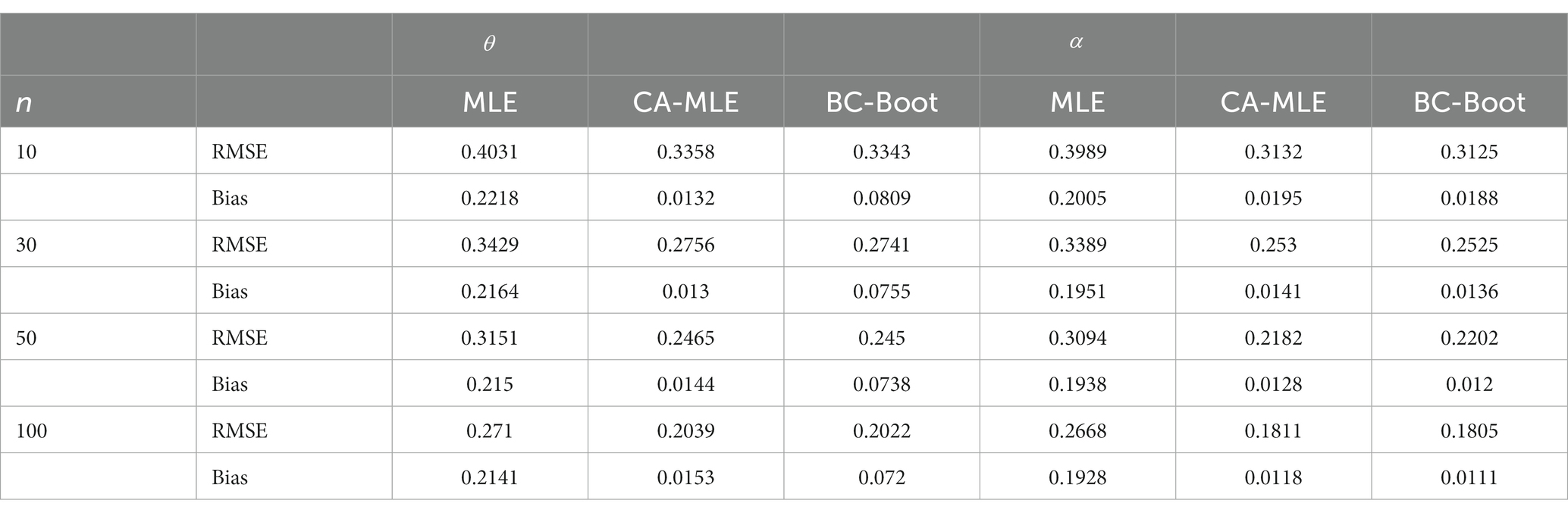
Table 1. Average RMSE and bias when $(θ = 1.5, α = 2)$ .

Table 2

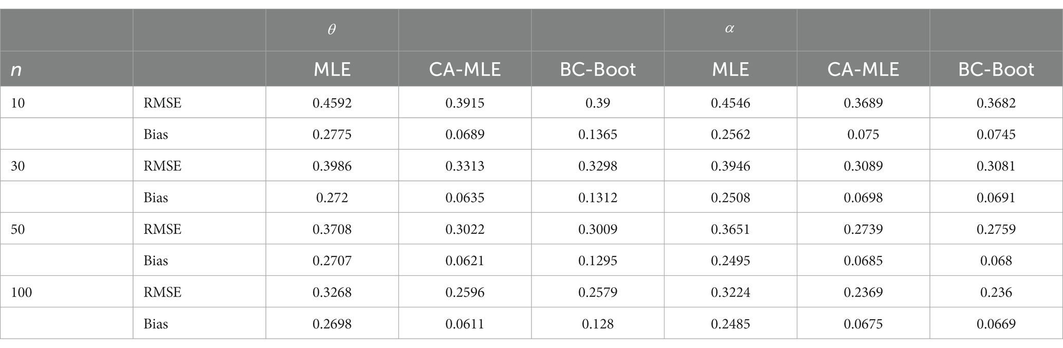
Table 2. Average RMSE and bias when $(θ = 2.2, α = 3)$ .

Table 3

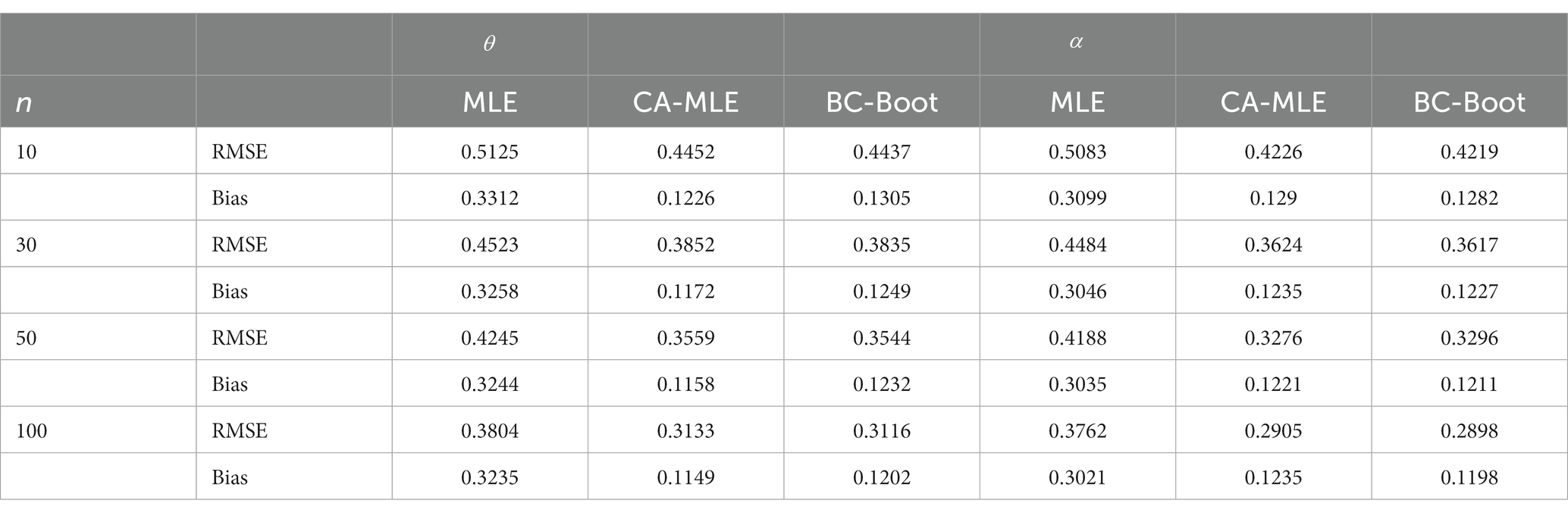
Table 3. Average RMSE and bias when $(θ = 5, α = 7)$ .

5 Real data application

In this part, we use two real datasets with a small sample to demonstrate the usefulness of the suggested BC estimators for the ETD distribution. The first dataset represents the life time failure of 18 electronic devices (45). This data was further analyzed by Wang and Wang (38). The second dataset represents the tubes that show leaks under a 120 psi stress level (46). The sample size of this data is 30. This data was further analyzed by Çetinkaya and Bulut (17).

To check whether the first and second data belong to the ETD distribution, the Kolmogorov–Smirnov test as a goodness-of-fit is used. The result of the test for the first data set is 6.281, with a p-value of 0.611. On the other hand, the result of the goodness-of-fit for the second data set equals 8.068, with a p-value of 0.744. These results indicate that the ETD distribution can fit very well with these data.

Tables 4, 5 show the estimated values for the parameters of the alpha power exponential distribution. Tables 4, 5 demonstrate that the CA-MLE and BC-Boot estimates of $θ$ and $α$ are less than the MLE estimate, indicating that the MLE approach overestimates this parameter.

Table 4

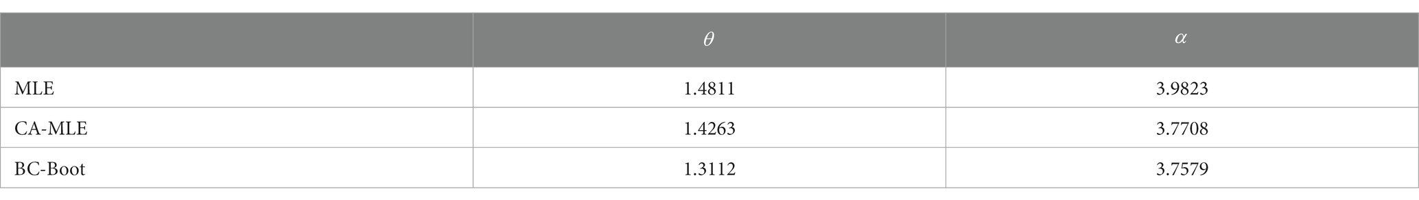
Table 4. Point estimates of the $θ$ and $α$ of ETD distribution for the electronic device data.

Table 5

Table 5. Point estimates of the $θ$ and $α$ of ETD distribution for the show leak data.

The analysis of the ETD distribution pdf in relation to Tables 4, 5 for $θ$ and $α$ values of both datasets is shown in Figures 1, 2, respectively. We suggest using CA-MLE and BC-Boot estimates for both datasets because the density shape based on the MLE method may be deceptive, as this figure illustrates.

Figure 1

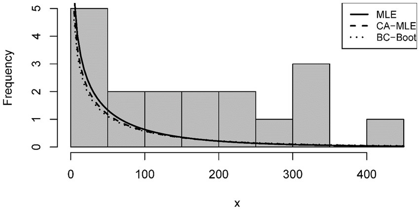
Figure 1. Estimated fitted density functions of the first dataset.

Figure 2

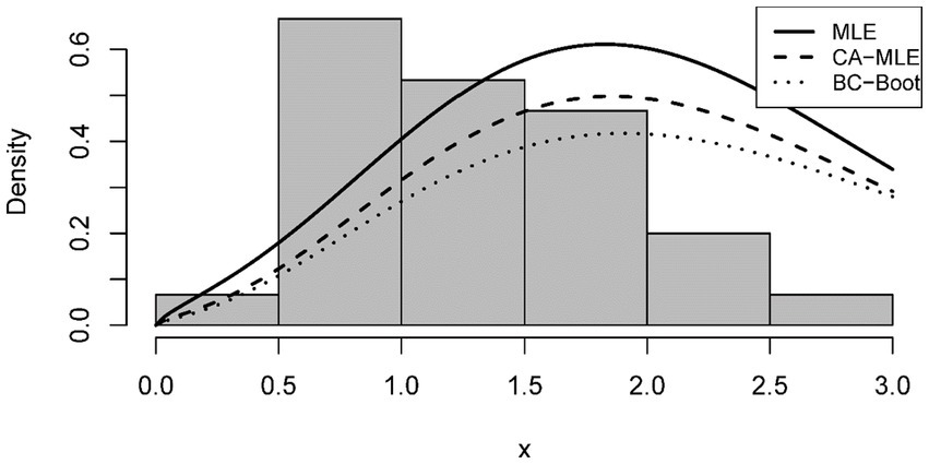
Figure 2. Estimated fitted density functions of the second dataset.

6 Conclusion

In order to obtain straightforward closed-form equations for the second-order biases of the MLE of the parameters of the ETD distribution, the corrective method was proposed in this paper. Namely: CA-MLE and BC-Boot. The newly proposed estimators converge to their real value significantly faster than the MLE, as evidenced by their biases being of order $O (n^{- 2})$ as opposed to $O (n^{- 1})$ for the MLE. The suggested approaches exceed the MLE in terms of bias and RMSE, as demonstrated by the numerical data, making them highly appealing. The suggested BC estimators are highly advised, particularly in cases where the sample size is small.

Data availability statement

The raw data supporting the conclusions of this article will be made available by the authors, without undue reservation.

Author contributions

AA: Formal analysis, Validation, Writing – original draft. ZA: Supervision, Writing – original draft, Writing – review & editing. OA: Methodology, Software, Writing – review & editing.

Funding

The author(s) declare that no financial support was received for the research, authorship, and/or publication of this article.

Conflict of interest

The authors declare that the research was conducted in the absence of any commercial or financial relationships that could be construed as a potential conflict of interest.

Publisher’s note

All claims expressed in this article are solely those of the authors and do not necessarily represent those of their affiliated organizations, or those of the publisher, the editors and the reviewers. Any product that may be evaluated in this article, or claim that may be made by its manufacturer, is not guaranteed or endorsed by the publisher.

Supplementary material

The Supplementary material for this article can be found online at: https://www.frontiersin.org/articles/10.3389/fams.2024.1351651/full#supplementary-material

References

1. Alanaz, MM, and Algamal, ZY. Neutrosophic exponentiated inverse Rayleigh distribution: properties and applications. Int. J. Neutrosophic Sci. (2023) 21:36–42. doi: 10.54216/IJNS.210404

ORIGINAL RESEARCH article

Bias reduction of maximum likelihood estimation in exponentiated Teissier distribution

1 Introduction

2 Maximum likelihood estimation

3 Bias-corrected MLEs

3.1 A corrective approach

3.2 Bootstrap approach

4 Simulation results

5 Real data application

6 Conclusion

Data availability statement

Author contributions

Funding

Conflict of interest

Publisher’s note

Supplementary material

References

People also looked at