Why strengthening gap junctions may hinder action potential propagation
 Erin Munro Krull
 Christoph Börgers
- 1Department of Mathematical Sciences, Ripon College, Ripon, WI, United States
- 2Department of Mathematics, Tufts University, Medford, MA, United States
Gap junctions are channels in cell membranes allowing ions to pass directly between cells. They are found throughout the body, including heart myocytes, neurons, and astrocytes. In cardiac tissue and throughout the nervous system, an action potential (AP) in one cell can trigger APs in neighboring cells connected by gap junctions. It is known experimentally that there is an ideal gap junction conductance for AP propagation—lower or higher conductance can lead to propagation failure. We explain this phenomenon geometrically in branching networks by analyzing an idealized model that focuses exclusively on gap junction and AP-generating currents. As expected, the gap junction conductance must be high enough for AP propagation to occur. However, if the gap junction conductance is too high, then it dominates the cell's intrinsic firing conductance and disrupts AP generation. We also identify conditions for semi-active propagation, where cells in the network are not individually excitable but still propagate action potentials.
1 Introduction
Gap junctions are found throughout the body [1–3]. In particular, gap junctions connect astrocytes [4], neurons [5–8], especially during development [9, 10] and heart myocytes [11–13]. More recently, gap junctions were observed in cancer cells [14, 15] and between soma and germline cells [16].
Gap junctions allow ions to pass between cells, and so the voltage in one cell directly influences the voltage in the neighboring cell. Suppose two excitable cells are connected, a “trigger” cell and a downstream neighbor, and both are at rest. If there is a small voltage deflection in the trigger cell, then we will see a proportional deflection in the neighbor. This proportion is often referred to as the coupling coefficient [17]. If the gap junction conductance is low, then an action potential (AP) in the trigger cell may only yield a subthreshold response in the neighbor. This response is called passive propagation since the neighbor's firing currents are never fully activated. On the other hand, if the gap junction conductance is high, then an AP in the trigger cell may yield an AP in the neighbor. We call this active propagation since the neighbor's firing currents amplify the response.
Active propagation of APs across gap junctions is seen in cardiac tissue [11–13] and throughout the nervous system [18–25]. More recently, gap junctions were found to mediate propagating calcium waves through smooth muscle tissues [26], neural progenitor cells [27], possibly astrocytes [28–30], and retinal cells [31].
Several studies have reported that APs propagate most easily across a given network for intermediate gap junction conductances; see Figure 1. Experiments in heart tissue show that reducing the gap junction conductance can allow APs to propagate through expanding tissue [12, 32, 33]. These results are corroborated in computational models of heart tissue, which show that there is an ideal gap junction conductance that maximizes the number of downstream neighbors that APs may propagate across [34] and that maximizes the “safety factor,” a measure of ease of propagation in terms of source-sink mismatch [34–38].
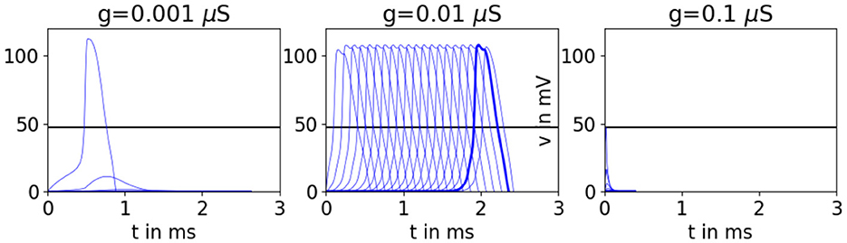
Figure 1. Simulations of Hodgkin-Huxley-type neurons [39] connected by gap junctions in a 20-layer tree network where each cell has one upstream neighbor and two downstream neighbors. The lead cell is stimulated until its voltage reaches approximately 1/2 the AP height of an unconnected cell, marked by a black horizontal line. (See section 4 for simulation details.) We see propagation failure when the gap junction conductance g is either too high or too low, and AP propagation when g is set to a medium amount.
To understand these results, we consider a network of cells connected by gap junctions with possibly many downstream neighbors. If the gap junction conductance between cells is zero, clearly APs cannot propagate through the network. As the gap junction conductance is raised, propagation becomes possible. However, if the conductance is raised too much, current shunted to downstream neighbors may prevent APs from propagating.
Extending the study in [40] and [41], we use a one-dimensional simplification of the FitzHugh-Nagumo equations to analyze when active AP propagation is possible in branching networks. In particular, our framework explains why increasing gap junction conductance may hinder AP propagation beyond pointing to a source-sink mismatch: AP propagation is the easiest when the total gap junction conductance is large enough to overcome the cell's intrinsic conductance below the firing threshold, but small enough to not interfere with the cell's conductance above the firing threshold. We illustrate this phenomenon for AP propagation into a single cell and branching networks. We then verify that our conclusions hold qualitatively for more realistic biophysical models. Our analysis also predicts that if the gap junction conductance reaches a threshold, we may see semi-active propagation where individual cells in the network cannot fire an AP independently from their neighbors, but the network can still propagate APs.
2 Propagation into a single cell
2.1 Model of a single cell
We model a single cell using the equation
where vT is a parameter with 0 < vT < 1. We let F(v) stand for the right-hand side of Eq. (1), illustrated in Figure 2. We think of v as a non-dimensionalized membrane potential and will therefore refer to it as voltage. We also think of F(v) as the inward activation current (more accurately, current divided by capacitance) and therefore may interpret F′(v) as the intrinsic conductance of the cell. Equation (1) is one half of the FitzHugh-Nagumo model [42]. We omit the other half, the slow variable that drives v down when it is high. Our focus, for now, is on the initiation, not on the termination of spikes. Single cell simulations in the Supplementary material show that slow gating variables do not appreciably change during AP initiation.
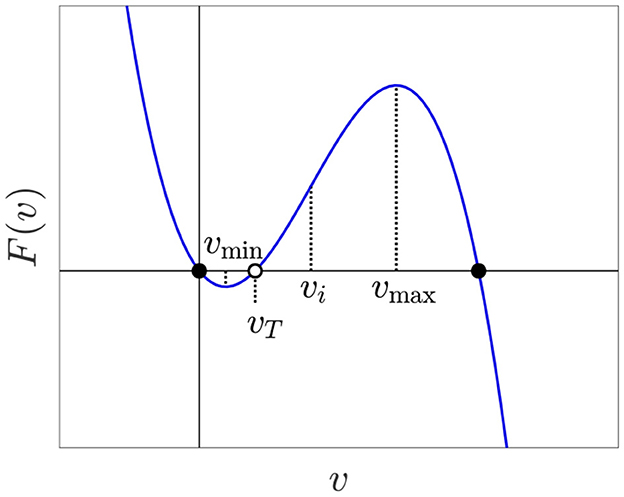
Figure 2. Graph of F with intrinsic threshold vT = 0.2.
Equation (1) has a stable equilibrium at v = vR = 0, an unstable one at v = vT representing the intrinsic threshold, and a stable one at v = vF = 1 representing the AP firing voltage. If v is perturbed slightly from 0, it returns to 0, but if it is raised above vT, it rises further to 1 instead. While we technically have a bi-stable differential equation, since we are using this model to focus on AP initiation, we still think of this as a model for excitability. In this study, excitability always means the co-existence of a stable resting state and an unstable threshold, with the property that perturbation away from the stable resting state and past the threshold results in a large excursion to the AP firing voltage. Once the voltage reaches the AP firing voltage, we assume the recovery currents of the full FitzHugh-Nagumo model would take the voltage back to rest.
The graph of F has a local minimum vmin and an inflection point at vi = (vT + 1)/3. We assume vT < vi, which is equivalent to
For neurons and myocytes, this is a natural assumption: The firing threshold is closer to the resting voltage (v = 0) than to the peak voltage (v = 1). So
as illustrated in Figure 2.
2.2 Gap junction connections with neighbors held at fixed voltage
Consider a cell described in the previous section that is connected by gap junctions to one upstream neighbor with voltage vu and k downstream neighbors with voltage vd = 0. The upstream and downstream voltages are assumed fixed for now. Only the central cell has dynamics. Simulations (not shown) verify that the assumption vd = 0 is reasonable as long as the central cell's voltage is below threshold. We assume that all gap junction conductances have the same strength g, and stimulation comes from the upstream neighbor. See Figure 3 for an illustration with k = 3.
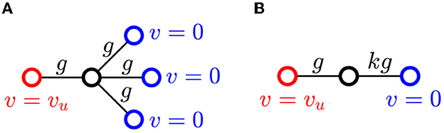
Figure 3. (A) Cell with upstream and downstream neighbors at fixed voltages. (B) By symmetry, we can collapse the downstream neighbors into a single cell.
Our model now becomes
As is customary, we assume here that gap junctions are governed by Ohm's law—current is proportional to voltage difference. The term g(vu − v) models the effect of the upstream cell and −gkv models the effect of the downstream cells. With the notation
Eq. (2) becomes
Figure 4A shows F and G in one figure. The graph of G intersects the horizontal axis at (vu/(k + 1), 0), and the vertical axis at (0, −gvu).
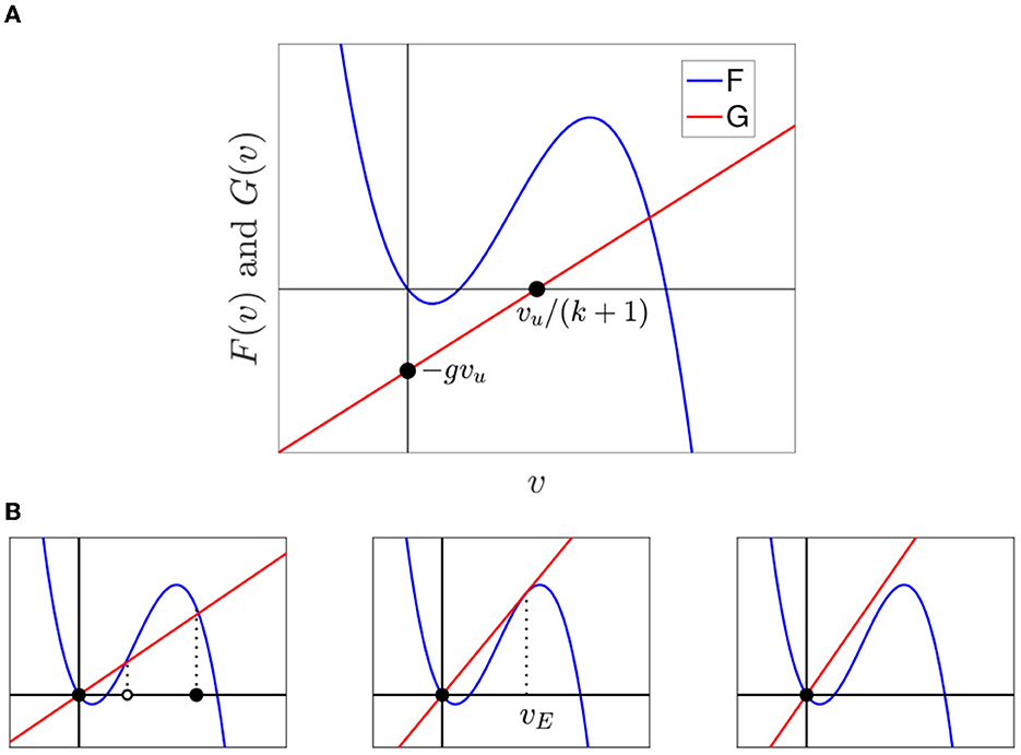
Figure 4. (A) Graph of F with the graph of G, a straight line with vertical intercept (0, −gvu) and v-intercept . In this example, vT = 0.2, g = 0.2, and k = 1. (B) F and G for vu = 0 at different values of g(k + 1).
In general, there may be more upstream cells than just one. There may also be more or fewer downstream cells coupled to the central cell with varying conductances. What matters is that g is the total gap junction conductance of connections between the central cell and upstream cells and kg is the total gap junction conductance of connections between the central cell and downstream cells. Therefore, we will not assume k to be an integer any more, simply thinking of it as the ratio of total downstream conductance over total upstream conductance.
2.3 All neighbors at rest
We first discuss the equilibria of the central cell when the upstream neighbors of the central cell are at rest (vu = 0) just like the downstream neighbors. The formula for G(v) is now
Fixed points of Eq. (2) are solutions of
If g(k + 1) is not too large, then there are three equilibria, depicted in the left panel of Figure 4B. As g(k + 1) increases, the graph of G becomes steeper. This raises the threshold vt and lowers the AP firing voltage vf but does not affect the resting voltage. Eventually, the threshold and firing equilibrium points collide at a voltage which we denote by vE; see the middle panel of Figure 4B. For larger g(k + 1), there is only one equilibrium at v = 0.
We say that the cell is excitable if there are three equilibria—an unstable threshold surrounded by two stable equilibria. This is consistent with the common notion of an excitable cell, where a small deflection in voltage across a threshold can cause a large excursion to a much higher voltage. Hence, the cell is excitable if
and is not for higher values of g(k + 1). So gap junction connections with neighbors held at rest, if they have high conductance or are numerous enough, can make excitability disappear altogether. We will see below that non-excitable cells can still amplify a response—just not independently from other cells.
2.4 Firing triggered by raising the upstream voltage
As vu is raised from 0 to some maximum value Vu > 0, the graph of G moves downward. Depending on the values of Vu, k, and g, the threshold and resting voltages may eventually collide and annihilate each other in a saddle-node bifurcation, leaving the AP firing voltage as the only equilibrium. We let vu,c be the bifurcation point, where vmin < vu,c < vi; see Figure 5A.
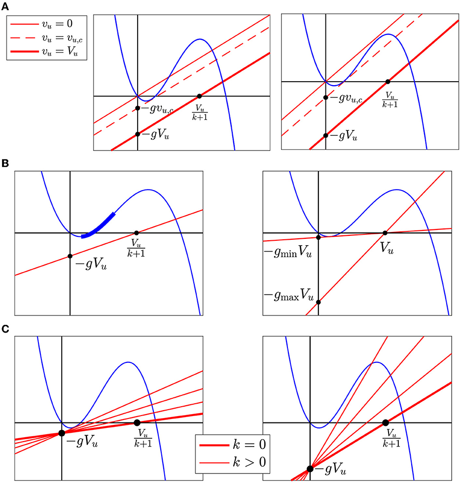
Figure 5. (A) Raising vu shifts the graph of G. (B) The left panel shows an example of an admissible line Lg,k. The critical segment is the bold blue segment along F. The right panel shows the lines Lg,k for the minimum and maximum values of g allowing a firing response. Both occur when k = 0. (C) The left panel shows an example where the maximum k occurs when Lg,k is tangent to the graph of F. The right panel shows an example where the maximum k occurs when Lg,k reaches .
As the right panel of Figure 5A shows, even when the central cell is not excitable because it is too strongly connected to resting neighbors, raising vu may restore excitability by making the threshold and AP firing voltage equilibria re-appear via a saddle-node bifurcation. Then, at vu = vu,c, the resting and threshold equilibria collide and disappear.
Definition 1. We say that the central cell fires or has a firing response when vu rises from 0 to Vu if there is a saddle-node bifurcation between the rest and threshold fixed points at some critical value vu = vu,c with vmin < vu,c < vi.
Definition 2. The critical segment is the segment between v = vmin and v = vi on the graph of F.
The left panel of Figure 5B shows the critical segment in bold. The collision between the rest and threshold fixed points must occur on the critical segment. Therefore, the following proposition holds.
Proposition 1. Let g > 0 and k ≥ 0. The central cell fires when vu is raised from 0 to Vu if and only if Lg,k (the graph of G with vu = Vu) satisfies the following two conditions.
(1) Lg,k lies strictly below the critical segment
(2) Lg,k has slope .
We say Lg,k is admissible if it satisfies the conditions in Proposition 1, as illustrated in the left panel of Figure 5B.
2.5 Region in (g,k)-plane with firing response
We use Proposition 1 to derive a detailed description of the set of the parameter pairs (g, k) for which the central cell has a firing response. First, we note that Lg,k cannot be admissible if Vu ≤ vT. We will therefore assume
Furthermore, since lowering k rotates Lg,k clockwise around the point (0, −gVu), lowering k makes it easier to fire: For Lg,k to be admissible for a given g, Lg,0 has to be admissible (this makes sense, since lowering k lowers the current shunted to the downstream neighbors). Therefore, we first analyze the case k = 0. Note that Lg,0 passes through (Vu, 0). For Lg,0 to be admissible, g must satisfy
where Lgmin, 0 is tangent to the critical segment and Lgmax, 0 has slope , as illustrated by the right panel of Figure 5B. Since the slope of Lg,0 is g, then .
Now, we consider k > 0. Suppose g lies between gmin and gmax. Then, Lg,0 is admissible. Other admissible lines, for the same value of g, are obtained by rotating this line around the point (0, −gVu) in the counter-clockwise direction until it touches the critical segment or reaches slope —whichever comes first.
Which of these two does come first depends on g. If g is smaller than some threshold value g* (discussed further below), then as the line rotates counter-clockwise around (0, −gVu), it touches the critical segment before it reaches slope ; see the left panel of Figure 5C. If g is larger than g*, the line reaches slope before it touches the critical segment; see the right panel of the figure.
From Figure 5C, we see that g* is determined by the tangent to F at (vi, F(vi)), which intersects the vertical axis at −g*Vu. That is,
Is it possible that ? According to (6), this means
or
The right-hand side of this inequality is the v-intercept of the tangent to F at (vi, F(vi))). So, g* ≥ gmax only if Vu happens to be very small, just above vT.
For every g ∈ (gmin, gmax), the slope g(k + 1) of the admissible line Lg,k is bounded above and the upper bound on g(k + 1) translates into an upper bound on k. So, the parameter regime where there is a firing response is of the form
and our next goal will be to understand what the graph of the function kmax looks like.
When g* ≤ g < gmax, the constraint on the slope of Lg,k is , and therefore
For gmin < g < g*, kmax(g) is obtained by computing the k where Lg,k is tangent to the critical segment. The two pieces match up continuously at g*, and we set
Our conclusions are summarized in Figure 6A. When Vu is so small that g* ≥ gmax, the dashed part of the blue boundary in Figure 6A is simply absent. The dotted and dashed parts of the upper boundary of the blue region in Figure 6A fit together continuously but not differentiably.
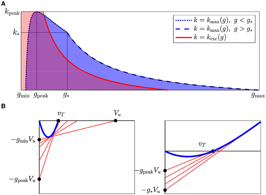
Figure 6. (A) Firing occurs in the region in the (g, k)-plane below kmax (blue), and the region where the cell is excitable with all neighbors at rest is below kexc (red). vT = 0.15, Vu = 1. (B) As g increases from gmin to g*, the v-intercept of the tangent through (0, −gVu) first moves left (left panel), then right (right panel). Therefore, kmax(g) first increases until reaches vT and then decreases.
In Figure 6A, we also indicate the regions in the (g, k)-plane, where the central cell is excitable when the upstream cell is at rest (vu = 0). From Eq. 5, the boundary of this region is defined by
We let kexc(g) stand for the right-hand side of (9) and describe how excitability affects behavior in more detail in section 2.7.
2.6 Ideal gap junction conductance
In Figure 6A, we see that kmax(g) reaches a maximum point at (gpeak, kpeak) at some g ∈ (gmin, g*). We also see that for all k < kpeak, as g increases AP propagation will first appear and then disappear as illustrated in Figure 1. To understand precisely how (gpeak, kpeak) corresponds to our model, we will examine what happens to Lg,k when it is tangent to the critical segment. In particular, we will follow what happens to the v-intercept (Vu/(kmax(g) + 1)) as g increases. As shown in Figure 6B, initially, the v-intercept falls as g increases until it reaches vT. As g continues to increase, the v-intercept rises again. Therefore, kmax rises until the v-intercept reaches vT and then falls. We can solve for (gpeak, kpeak) by setting Vu/(kpeak + 1) = vT, and therefore
and since ,
In other words, AP propagation is the easiest when the total conductance g(k + 1) is the same as the cell's intrinsic conductance when v = vT. At lower conductances, the gap junction current may not overcome the cell's current below threshold. At higher conductances, the gap junction current may interfere with the cell's firing currents.
2.7 Active, semi-active, and passive propagation
In Figure 6A, we see several distinct regions defined by kmax(g) and kexc(g). Notably, kexc(g) intersects kmax(g) so that a cell may fire without being excitable. Here, we describe these parameter regions.
Definition 3. The propagation region is the region of parameter pairs (g, k) with 0 ≤ k < kmax(g). The active propagation region is the section of the propagation regions where k < kexc(g), while the semi-active propagation region is the section where k ≥ kexc(g). The passive propagation region is the region where k ≥ kmax(g).
When (g, k) lies in the active propagation region (illustrated in Figure 6A where the red and blue regions overlap), the central cell is excitable for vu = 0 and fires when vu is set to Vu. When (g, k) lies in the semi-active propagation region, the central cell is not excitable for vu = 0, but as vu rises from 0 to Vu, first excitability is restored, and then there is a firing response. In the passive propagation region, raising vu from 0 to Vu still causes the voltage of the central cell to rise but does not trigger firing.
To illustrate the difference between the three parameter regions, Figure 7A shows solutions of (2) with v(0) = 0 and
In the active propagation region, the central cell's voltage rises and converges to the AP firing voltage, indicating an AP would occur in the full FitzHugh-Nagumo model. (Recall that our model includes no explicit mechanism for bringing the voltage back down after firing.) In the semi-active propagation region, the central cell's voltage also rises but drops back down to rest once vu is set back to 0—no matter how high the central cell's voltage gets. In the passive propagation region, the voltage rises much less and returns to zero soon after vu is switched back to zero.
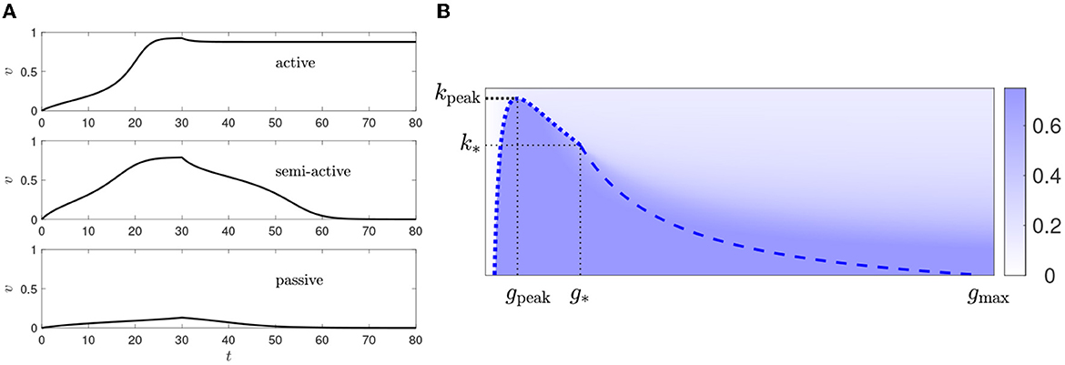
Figure 7. (A) Responses to setting vu = 1 for 0 ≤ t ≤ 30 and then setting it back to 0, for k = 2 and g = 0.03 (top), g = 0.07 (middle), and g = 0.01 (bottom). (B) Heat plot of v∞ as a function of g and k for vT = 0.15, Vu = 1. The blue curves are from Figure 6A. We see that v∞ is discontinuous along the dotted blue curve but not along the dashed blue curve.
2.8 AP height can depend discontinuously on g and k
For g > 0 and k ≥ 0, let v = v(t) be the solution of (2) with vu = Vu and v(0) = 0. Let
In other words, v∞ is the voltage obtained by setting the voltage in the upstream cell to Vu, letting the voltage in the central cell equilibrate, starting at v = 0; so, v∞ is the smallest equilibrium. We view v∞ as a function of g and k, as illustrated in Figure 7B. Notably, there is a discontinuous jump along the boundary defined by kmax (the dotted blue curve). This boundary is discontinuous in general, as stated in the following theorem.
Theorem 1. v∞(g, k) has jump discontinuities at parameter pairs (g, k) with gmin ≤ g < g* and k = kmax(g) and is continuous everywhere else.
Proof. Let g > 0 and k ≥ 0. As before, denote by Lg,k the graph of G with vu = Vu. Then, v∞(g, k) is the v-coordinate of the left-most intersection point of Lg,k and the graph of F. As illustrated in Figure 5A, v∞ depends discontinuously on (g, k) if and only if Lg,k is tangent to the graph of F along the critical segment. The (g, k) for which Lg,k is tangent to the graph of F at the critical segment are precisely the ones that define kmax(g) where g < g*.
3 Propagation through branching networks
3.1 Model
For motivation, first think about AP propagation through a tree of cells connected by gap junctions, as shown in Figure 8A. Assume that the cells are identical and each cell has exactly one upstream and k downstream neighbors. Propagation is triggered by raising the voltage of the leftmost cell to v = 1.
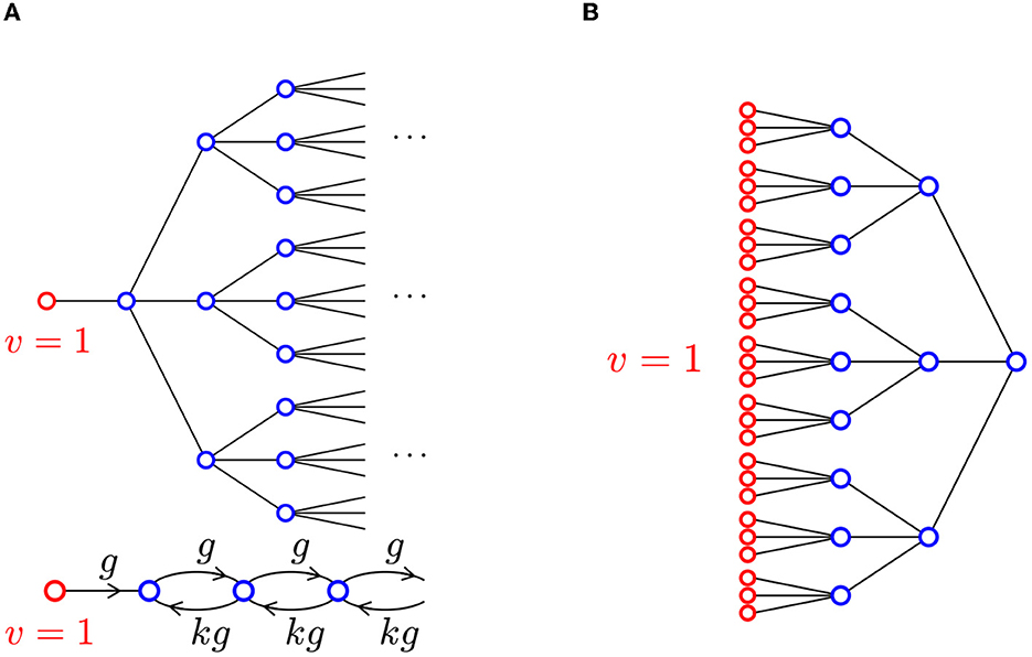
Figure 8. (A) A tree network, where each cell has one upstream neighbor and k = 3 downstream neighbors. Propagation is triggered by setting the voltage in the left-most cell to v = 1 (highlighted in red). The equivalent collapsed network is shown below. (B) A branching network where each cell has three upstream neighbors and one downstream neighbor, so k = 1/3. The collapsed network is the same as panel A but now k < 1.
By symmetry, the voltages in cells that are vertically aligned in Figure 8A are identical. We therefore collapse vertically aligned cells into a single cell and obtain the equivalent chain shown at the bottom of Figure 8A. In this chain, gap junction conductances are not symmetric: g for upstream connections and kg for downstream connections.
As we did earlier, we now drop the assumption that k is an integer, viewing it more abstractly as the ratio of downstream conductance over upstream conductance. We even allow k to be less than 1. This models a situation in which a signal originates from a large array of cells, propagating into a narrowing network: Think of a signal propagating through a tree from the tips of the outermost branches to the root, as shown in Figure 8B. We therefore consider the collapsed chain in Figure 8A as a mathematical idealization of many different kinds of branching networks.
We make the additional simplification that each cell responds only to the voltage upstream of it and behaves as though its downstream neighbors were held at zero voltage; its voltage therefore rises to v∞, as defined in Eq. 12. Propagation through the chain amounts to iterating the map
which maps [0, 1] into [0, 1].
3.2 AP propagation determined by sequence of max voltages
A complication in our analysis is that the map φ need not be continuous. To see this, first note that for any equilibrium v∞ of eq. (2), that is, for any solution v∞ of
we can solve for vu in terms of v∞:
We denote the right-hand side of this equation by ψ(v∞); Figure 9A shows an example. The graph of φ is obtained by swapping the v∞- and vu-axes, and using the minimum value of v∞ for a given vu when there is ambiguity; see Figure 9B.
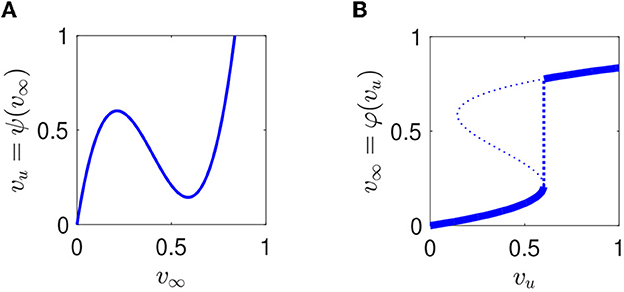
Figure 9. (A) Function ψ mapping equilibria of Eq. (2) onto vu. In this example, vT = 0.2, g = 0.058, and k = 2. (B) Corresponding function φ mapping vu onto the smallest equilibrium of Eq. (2), highlighted in bold.
Because of the discontinuity, we will not use the standard theory of iterated one-dimensional maps to understand the effect of iterating φ, but explicitly construct the iterates. Starting with v0 = 1, we define v1, v2, … by vj+1 = φ(vj) and j = 0, 1, 2, …. Given vj, vj+1 is the smallest solution of F(v) + g(vj − v) − gkv = 0 or
The graph of the right-hand side of this equation is the line Lg,k with Vu = vj, which passes through the point (vj, gkvj). To find vj+1 from vj, we first draw the line P(v) = gkv as a reference and then draw Lg,k through the point (vj, gkvj). The v-coordinate of the smallest intersection of Lg,k with F is vj+1. The construction of vj+1 from vj is illustrated by Figures 10A–C.
Figure 10. (A–C) Construction of vj+1 = φ(vj) starting with v0 = 1. For each iterate, we follow the dotted black line up to P(v) = gkv (black solid line) and then Lg,k (red solid line) down to the lowest intersection with F. In (A) P does not intersect F above v = 0 and so the iterates of φ converge to 0. In (B) P intersects F above v = 0, but Lg,k through the point (v0, gkv0) is not admissible and so the iterates of φ also converge to 0. In (C) P intersects F above v = 0 and all Lg,k through (vj, gkvj) are admissible, so the iterates of φ converge to v+ (the highest intersection between P and F). (D) Definitions of v+, v−. Note that v− ≤ vE ≤ v+, where vE is illustrated in Figure 4. (E) Illustration of the condition for persistent propagation. The line P(v) = gkv (black) must intersect, or at least tangentially touch, F(v) to the right of v = 0, and Lg,k through the point (v+, F(v+)) (red) must clear the critical segment, or at most touch it tangentially. (F) Construction of gmin, below which no persistent propagation is possible.
From Figure 10, we read off the following theorem on the convergence of the vj. In this theorem, vE is defined as in Section 2.3 (Figure 4).
Theorem 2. Suppose and v+ is the maximum solution to F(v) = gkv. Then if the line Lg,k through (v+, F(v+)) is admissible or is tangent to F(v) along the critical segment. In all other cases, .
If , we say that there is persistent propagation. If the line Lg,k through (v+, F(v+)) is tangent to F(v), we say it satisfies the tangency condition.
3.3 The region of persistent propagation
Our aim now is to understand for which values of g and k—that is, for which total upstream gap junction conductances and degree of expansion in our branching network—there can be persistent propagation. The result will be that the region of persistent propagation in the (g, k)-plane is of the form g ≥ gmin and 0 ≤ k ≤ kprop(g), as shown in Figure 11. In particular, there is an “ideal” conductance which maximizes the k that can support persistent propagation.

Figure 11. Region of propagation in the (g, k)-plane for vT = 0.2. The dotted part of the curve indicates where kprop(g) is determined by the tangency condition; the dashed part indicates where .
The geometric construction described by Figures 10A–C and theorem 2 mean that there is persistent propagation precisely if the line P(v) = gkv (depicted in black in Figure 10E) intersects or at least touches F(v) at some positive value v+ ≥ vE and with vu = v+ (depicted in red) lies below the critical segment or at most touches it in a single tangency point.
To better understand the shape of the region of persistent propagation (Figure 11), we fix g and ask how Figure 10E changes as k is increased (illustrated in Figure 12). The slopes of both P(v) (black) and Lg,k (red) increase with k. Because the slope of P(v) increases, v+ decreases. Therefore, the vertical intercept of Lg,k (−gv+) also increases. This implies that Lg,k rises and is closer to the critical segment if it was admissible before.
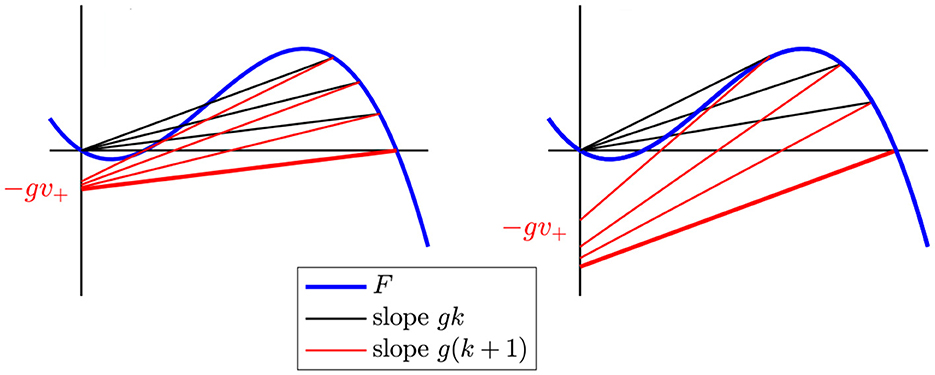
Figure 12. Left: For small g, the largest k for which there is persistent propagation is determined by the condition that the line Lg,k through (v+, gkv+) with slope g(k + 1) touches F tangentially. Here, we see P(v) and Lg,k for k = 0 (highlighted in bold) and then see how P(v) and Lg,k move as k increases, until Lg,k is tangent to F. Right: For large g, the largest k for which there is persistent propagation is determined by the condition . Again, the case k = 0 is highlighted in bold.
We conclude that for a fixed g, the range of values of k that allow persistent propagation is either empty or an interval of the form [0, kprop(g)] with kprop(g) ≥ 0. In particular, if there is persistent propagation for any k at all, there is persistent propagation for k = 0. Since the vertical intercept of Lg,0 (red) is −g, the minimum possible g is gmin, where Lgmin, 0 is tangent to the critical segment (Figure 10F).
For a given g > gmin, we obtain the range of values of k for which there is propagation by watching how P(v) = gkv and Lg,k (black and red lines) rotate as k increases, starting at k = 0. Figure 12 shows two examples. This leads to the following result.
Theorem 3. The region of persistent propagation in the (g, k)-plane is defined by
where Lgmin, 0 is tangent to the critical segment and kprop is continuous with kprop(gmin) = 0. For small g, kprop is defined by the tangency condition (described in Theorem 2 and illustrated in Figure 10E). For large g, .
Since kprop is 0 at gmin and tends to zero as g → ∞, there is always a value of g that is “optimal” for propagation in the sense that kprop is maximal. Figure 11 shows the region of propagation for vT = 0.2. Numerical simulations suggest that the peak still occurs approximately where . This reflects our results for a single cell, that AP propagation is the easiest when the total gap junction conductance and cell's intrinsic conductance at the threshold balance.
4 Comparison with more realistic models
We apply our analysis to see if we can predict AP propagation in simulations using more realistic models of a neuron and a cardiac myocyte. We use a four-dimensional Hodgkin-Huxley-type model of the neuronal axon [39], which serves as a base model for hippocampal axons connected by gap junctions in several studies [43, 44]. For the cardiac myocyte, we use the eight-dimensional Luo-Rudy model [45], which captures many of the complexities in the cardiac action potential [46]. We used Anaconda Jupyter notebooks [47] with Python 3 to run simulations and apply our analysis. Numerical simulations were conducted using solve_ivp in the Scipy Integrate library (version 1.10.1, [48]) using implicit differentiation specified by the ‘BDH' option. The code for all simulations and analysis are available in the Supplementary material.
4.1 A neuronal model
To start, we compare the single cell analysis of Section 2 with simulation results for a model of the neuronal axon. We consider a single cell with downstream neighbors held at rest (vR = 0 in [39]). To apply our analysis, we construct the activation curve for this model, FHH, by taking the right-hand-side of the voltage differential equation and replacing m with m∞(v), and keeping n and h (which are slower than v near vR) fixed at resting values. Using FHH, we calculate vF, the AP firing voltage of the disconnected cell, and vE, the maximum possible threshold voltage (see Figure 4 and the Supplementary material).
Using the full four-dimensional model, we run simulations of a single cell connected to fixed up- and downstream neighbors (Figure 3) for many (g, k) pairs under two different conditions:
1. The upstream cell is held at v = vF for the entire simulation.
2. The upstream cell is held at v = vF until the cell's voltage reaches vE.
For each simulation, we calculate the maximum voltage of the cell over the entire simulation for conditions 1 and 2. If the cell's voltage rises beyond vE under both conditions, then we say that active propagation is possible. However, if the cell's maximum voltage goes beyond vE only under the first condition, then only semi-active propagation is possible since the cell cannot maintain a full AP on its own. These results are shown in Figure 13A.
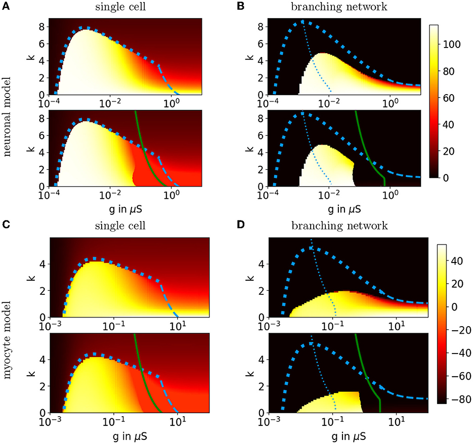
Figure 13. Behavioral regions for a Hodgkin-Huxley-type neuronal model and the Luo-Rudy myocyte model. (A) The heat map in the top graph shows the maximum voltage in mV over the entire simulation for a single Hodgkin-Huxley-type neuron where the upstream cell's voltage is held at vu = vF. The heat map in the bottom graph shows the maximum voltage when we only hold vu = vF until v = vE and then set vu = 0. Both heat maps range from vR to vF. The dashed blue curves show the predicted kmax. The solid green curve shows the predicted active-passive boundary kexc. (B) The heat maps show the maximum voltage in mV for the penultimate cell in a branching network of Hodgkin-Huxley-type neurons, where v0 = vF for the entire simulation in the top graph and v0 = vF only until v1 = vE in the bottom graph. Both heat maps range from vR to vF. The curves kprop (dashed blue), (dotted blue), and kexc (solid green) are both adjusted for the assumption that the downstream cell's voltage is proportional to the cell's voltage. (C, D) Single cell and branching network results for the Luo-Rudy myocyte model. Interestingly, the shape of the simulated propagation region in the branching network is different than the predicted shape and the shape for a single cell possibly due to activation of slower calcium currents.
We then calculate kmax(g) and kexc(g) using FHH, and compare them directly to the simulation results. Figure 13A shows that kmax(g) for a single cell matches the simulated active propagation region boundary quite well for small g, with a discontinuous jump in the voltage height up to g*. While the simulated boundary for the semi-active propagation is sharp as predicted in our framework, the simulated boundary lies to the left of the predicted boundary. The boundary matches the simulated active propagation regions, especially for g < g*, which confirms that fast activation currents are primarily responsible for AP initiation in a single cell.
For the branching network, we make modifications in both the analysis and the simulations. In the simulations, we model 20 layers of cells and record the maximum voltage of the penultimate cell to indicate whether APs propagated through the network. We also only hold downstream neighbors for the last cell fixed at v = 0. In our analysis, we therefore adjust the assumption that downstream neighbors are held at v = 0. Instead, we make a cell's downstream neighbor voltages proportional to the cell's voltage [49], which follows the steady-state condition when there are only passive currents. The details of this modification are explained in the Appendix in the Supplementary material.
In Figure 13B, we see that the simulated active propagation region for the branching network lies entirely within the predicted region and has a similar shape. That kprop over-estimates the boundary for AP propagation is to be expected since our analysis does not take the duration of an AP into account. (Though higher-order factors may shape the region as well, see section 5.) Regardless, we may still use the curve to estimate the peak, where the total gap junction conductance matches the cell's conductance at the intrinsic threshold. In Figure 13B, we see that the peak of the simulated active propagation region lies to the right of the peak curve. As predicted, there is a sharp boundary between the simulated semi-active propagation and active propagation regions. However, kexc(g) lies to the right of the simulated boundary. Figure 14 illustrates the behavior seen in each region of Figure 13B for k = 2, and Figure 15 gives an example of AP propagation on both sides of the simulated semi-active propagation boundary. In particular, in Figure 15, we see APs propagate in the branching network only if cells in multiple layers are depolarized enough to fire.
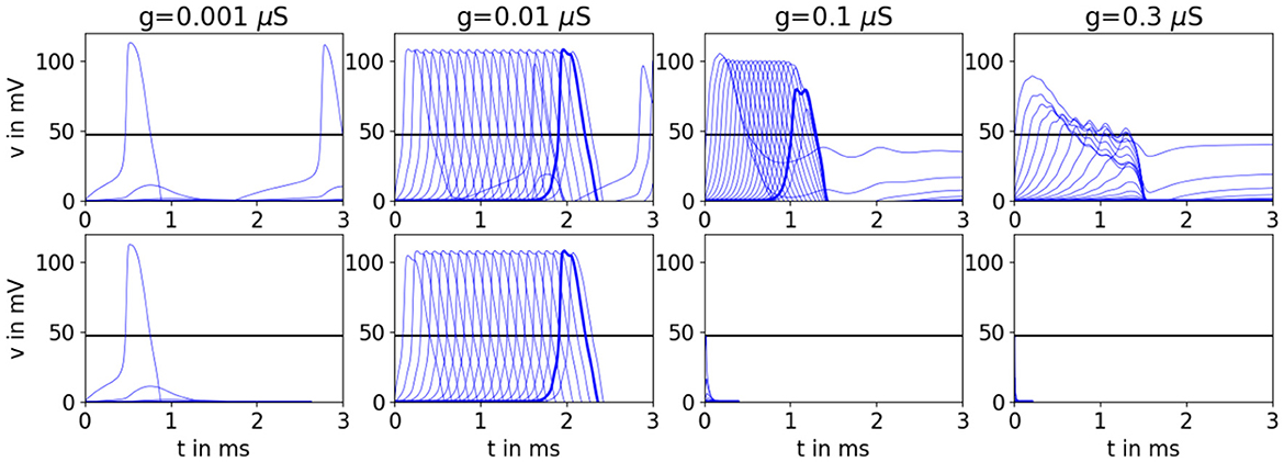
Figure 14. Simulations of the branching network for Hodkin-Huxley-type neurons with k = 2 showing the full range of behaviors. The top row shows results for condition 1, while the bottom panel shows results for condition 2 (also shown in Figure 1). In Figure 1, we saw propagation failure for g = 0.1 μS. In this figure, we see that the network will propagate if we hold the stimulation until more of the network is depolarized. However, we will always get propagation failure for very high values of g, such as g = 0.3 μS. The black horizontal line marks vE. There are 20 cell layers in the network. The penultimate cell is highlighted in bold.
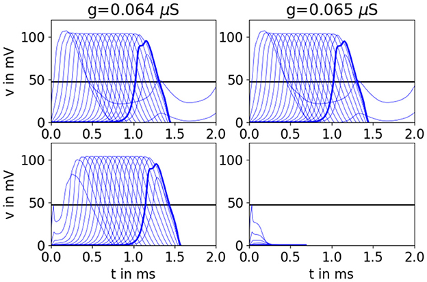
Figure 15. Simulations on both sides of the semi-active propagation boundary reveal that AP propagation may depend on depolarization of multiple downstream cells. Simulations of the branching network for Hodkin-Huxley-type neurons with k = 2. Top panels show results for condition 1, bottom panels show results for condition 2. Under condition 2 on the left, the first cell's voltage dips down immediately after stimulation ends but is eventually pulled up when multiple layers fire. On the right, the downstream cells pull the first cell down, and they never recover. They all fail to propagate an AP at once. The black horizontal line marks vE. There are 20 cell layers in the network. The penultimate cell is highlighted in bold.
4.2 A myocyte model
We compare simulations using the full eight-dimensional Luo-Rudy myocyte model [45] to our analysis in a similar manner to the neuron model above. We construct the activation curve FLR by replacing m with m∞(v) and holding all other gating variables (which are slower than v near vR) fixed at their resting values. For ease of calculation, we also re-center FLR(v) so that the resting fixed point is vR = 0. Using the same simulation setup as in section 4.1, in Figures 13C, D, we again see that simulated AP propagation into a single cell matches the predicted boundaries very well, especially for small g. Similarly, for the branching network, the simulated active propagation region lies entirely within the predicted boundary but does not quite have a similar shape. This may be due to the fact that slower calcium currents in the Luo-Rudy myocyte model allow APs to propagate for low g [38]. Similar to the neural model, the peak of the simulated active propagation region lies to the right of the peak curve. There is a sharp boundary between the semi-active and active propagation regions, which lies to the left of the predicted boundary.
5 Discussion
We explained why AP propagation through a branching network of excitable cells connected by gap junctions depends non-monotonically on gap junction conductance. We did this by reducing models to one-dimensional firing currents, which allows us to visualize how the firing currents and gap junction currents interact. From this visualization, we estimate that AP propagation is easiest when the total gap junction conductance matches the cell's conductance at its intrinsic threshold. We also found a discrete behavioral region where cells may propagate APs but are so strongly connected that they are no longer individually excitable.
We believe this framework can give a simple and efficient method for understanding where AP propagation may occur and may add guidelines on whether to raise or lower gap junction conductance to enhance propagation. For example, cells in realistic networks have a heterogenous number of connections. Our framework may predict when AP propagation failure and subsequent re-entry occurs at cells with higher connectivity [12, 43, 50]. Currently, simulations are used to determine whether APs will propagate through any given network. For instance, whole heart simulations are a promising diagnostic tool in heart patients but can be computationally costly [51]. While cellular automata may alleviate the computational cost [52], our framework can inform phenomenological rules and greatly reduce the parameter space that needs to be searched. Finally, our framework outlines how the AP height, threshold, and subthreshold response changes with gap junction conductance [53]. These measures may be useful in determining the state of a network and predicting network-wide phenomena such as synchronization.
Moreover, this framework may be used to understand how network behavior may change with changes in connectivity, gap junction conductance, and firing currents. Cardiac arrhythmia can be brought about by pathogenic stressors [54, 55], adrenergic stimulation [56], or myocardial ischemia (buildup of plaques) associated with decreased gap junction coupling [57, 58]. Abnormal gap junction ubiquitination can affect both the heart and nervous system [59]. Gap junctions may be sensitive to toxins [60]. Epilepsy has been tied to gap junctions connecting networks of pyramidal cell axons, interneurons, and astrocytes, each of which play a different role in network excitability [61–64]. Furthermore, gap junctions are indicated in Parkinson's disease [65], Alzheimer's disease [66], nerve injury [67–69], and degenerative diseases in the retina [70]. Modulating gap junction conductance may help with several of these conditions; however, questions remain on how much gap junctions can be modulated without producing adverse side effects [71, 72]. An alternative may be to modulate firing currents through gene therapy [73]. There are also many conditions where external stimulation is applied as a part of therapeutic treatment [51, 74–77]. We hope that our framework can give insight on appropriate ranges to maintain proper function in a variety of networks.
Our study is closely related to several other studies. We directly extend the theory presented by Keener [40], which addresses the conditions where AP propagation may occur in a chain of cells with no branching. Our study also extends the study of Kouvaris et al. [41], who analyzed a bistable system where both the high and low resting voltages are fixed. This matches our analysis for AP propagation into a single cell, so their bifurcation diagram matches our bifurcation diagram for a single cell (Figure 6). We take a more geometric approach, which clearly shows that the analysis depends only on the qualitative shape of the activation curve. This allows us to analyze the peak value of k for AP propagation. We also show how connectivity affects the AP firing voltage, which then determines whether persistent propagation is possible. Wang and Rudy first showed a biphasic relationship between gap junction conductance and an expansion ratio using simulations of cardiac tissue [34]. Several experimental and computational studies show a biphasic relationship between gap junction conductance and the safety factor [34, 38, 78, 79]. While our framework can predict where AP propagation is possible, the safety factor measures the source-sink mismatch from a recording or simulation based on the incoming current vs. outgoing current in a single cell. Finally, there are other studies that show an ideal gap junction conductance for propagation using a mean-field model [80], in a network using small-world topology [81], and an ideal cable diameter for AP propagation [82, 83].
We note that our framework only provides simple guidelines outlining where AP propagation may occur. While this theory can give a first estimate on when to expect AP propagation, there are many ways we could increase the accuracy of this prediction. For instance, we could link different versions of φ(v) to model AP propagation through a network with heterogenous numbers of downstream neighbors. We may also improve the prediction by taking the connectivity of downstream neighbors more fully into account. In fact, AP propagation may not only depend on the number of immediate downstream neighbors, but on the number of neighbors several steps away [43]. Future studies may incorporate multiple layers of downstream neighbors. The predicted AP propagation regions in our framework overestimate the regions found in the original models. Preliminary results show that for the Fitzhugh-Nagumo model, the simulated boundary may be better predicted by taking into account the time to reach the threshold. However, a correction based on the timing still does not quantitatively predict the region in higher-order models. This may be due to higher-dimensional interactions within the cell, such as calcium currents in the Luo-Rudy myocyte model which may allow APs to propagate for low g [38].
Our framework studies propagation assuming the first cell is firing. It does not address getting the first cell to fire in the first place but rather reproduces the situation where the cell is voltage clamped. As gap junction conductance increases, it may take an increasing amount of current to bring the first cell to the desired voltage. In some cases, we may need to depolarize multiple downstream neighbors in the network to get AP propagation, similar to what is seen in semi-active propagation.
Overall, reduction of cell models to one-dimensional firing currents gives insight into how gap junction currents allow active propagation, semi-active propagation, or passive propagation. The shape of the firing currents explains how the threshold and peak firing voltage change with gap junction conductance and allows us to approximate an ideal gap junction conductance for AP propagation. This framework gives further insight into the mechanisms of these networks - which play a key role in both normal biophysiological function and disease.
Data availability statement
The original contributions presented in the study are included in the article and Supplementary material. Further inquiries can be directed to the corresponding author.
Author contributions
EM developed the original concept and analysis. EM and CB revised the analysis and visualization and wrote and edited the manuscript.
Funding
We thank Tufts University for paying for the open access page charges through a Faculty Research Awards Committee (FRAC) grant. EM was partially funded by a National Science Foundation (NSF) Mathematical Sciences Postdoctoral Research Fellowship, NSF Award Number 0802889.
Acknowledgments
The authors thank Nancy Kopell for many insightful comments on this study, and students who participated in this research, especially Abel Gonzalez and Mitra Kermani.
Conflict of interest
The authors declare that the research was conducted in the absence of any commercial or financial relationships that could be construed as a potential conflict of interest.
Publisher's note
All claims expressed in this article are solely those of the authors and do not necessarily represent those of their affiliated organizations, or those of the publisher, the editors and the reviewers. Any product that may be evaluated in this article, or claim that may be made by its manufacturer, is not guaranteed or endorsed by the publisher.
Supplementary material
The Supplementary Material for this article can be found online at: https://www.frontiersin.org/articles/10.3389/fams.2023.1186333/full#supplementary-material
Presentation 1. Appendix.
Data Sheet 1. Code for all simulations and analysis.
References
2. Goodenough DA, Paul DL. Gap junctions. Cold Spring Harb Perspect Biol. (2009) 1:a002576. doi: 10.1101/cshperspect.a002576
3. Rackauskas M, Neverauskas V, Skeberdis VA. Diversity and properties of connexin gap junction channels. Medicina (Kaunas). (2010) 46:1–12. doi: 10.3390/medicina46010001
4. Bennett MVL, Contreras JE, Bukauskas FF, Sez JC. New roles for astrocytes: gap junction hemichannels have something to communicate. Trends Neurosci. (2003) 26:610–7. doi: 10.1016/j.tins.2003.09.008
5. Bennett MVL, Zukin RS. Electrical coupling and neuronal synchronization in the mammalian brain. Neuron. (2004) 41:495–511. doi: 10.1016/S0896-6273(04)00043-1
6. Connors BW, Long MA. Electrical synapses in the mammalian brain. Annu Rev Neurosci. (2004) 27:393–418. doi: 10.1146/annurev.neuro.26.041002.131128
7. Hormuzdi SG, Filippov MA, Mitropoulou G, Monyer H, Bruzzone R. Electrical synapses: a dynamic signaling system that shapes the activity of neuronal networks. Biochim Biophys Acta. (2004) 1662:113–37. doi: 10.1016/j.bbamem.2003.10.023
8. Söhl G, Maxeiner S, Willecke K. Expression and functions of neuronal gap junctions. Nat Rev Neurosci. (2005) 6:191–200. doi: 10.1038/nrn1627
9. Montoro RJ, Yuste R. Gap junctions in developing neocortex: a review. Brain Res Brain Res Rev. (2004) 47:216–26. doi: 10.1016/j.brainresrev.2004.06.009
10. Sutor B, Hagerty T. Involvement of gap junctions in the development of the neocortex. Biochim Biophys Acta. (2005) 1719:59–68. doi: 10.1016/j.bbamem.2005.09.005
11. Bernstein SA, Morley GE. Gap junctions and propagation of the cardiac action potential. Adv Cardiol. (2006) 42:71–85. doi: 10.1159/000092563
12. Kleber AG, Jin Q. Coupling between cardiac cells an important determinant of electrical impulse propagation and arrhythmogenesis. Biophys Rev. (2021) 2:031301. doi: 10.1063/5.0050192
13. Roerig B, Feller MB. Neurotransmitters and gap junctions in developing neural circuits. Brain Res Brain Res Rev. (2000) 32:86–114. doi: 10.1016/S0165-0173(99)00069-7
14. Bonacquisti EE, Nguyen J. Connexin 43 (Cx43) in cancer: implications for therapeutic approaches via gap junctions. Cancer Lett. (2019) 442:439–44. doi: 10.1016/j.canlet.2018.10.043
15. Osswald M, Jung E, Sahm F, Solecki G, Venkataramani V, Blaes J, et al. Brain tumour cells interconnect to a functional and resistant network. Nature. (2015) 528:93–8. doi: 10.1038/nature16071
16. Landschaft D. Gaps and barriers: gap junctions as a channel of communication between the soma and the germline. Semin Cell Dev Biol January. (2020) 97:167–71. doi: 10.1016/j.semcdb.2019.09.002
17. Welzel G, Schuster S. A direct comparison of different measures for the strength of electrical synapses. Front Cell Neurosci. (2019) 13:43. doi: 10.3389/fncel.2019.00043
18. Chorev E, Brecht M. In vivo dual intra- and extracellular recordings suggest bidirectional coupling between CA1 pyramidal neurons. J Neurophysiol. (2012) 108:1584–93. doi: 10.1152/jn.01115.2011
19. Draguhn A, Traub RD, Schmitz D, Jefferys JGR. Electrical coupling underlies high-frequency oscillations in the hippocampus in vitro. Nature. (1998) 394:189–92. doi: 10.1038/28184
20. Mercer A, Bannister AP, Thomson AM. Electrical coupling between pyramidal cells in adult cortical regions. Brain Cell Biol. (2006) 35:13–27. doi: 10.1007/s11068-006-9005-9
21. Papasavvas CA, Parrish RR, Trevelyan AJ. Propagating activity in neocortex, mediated by gap-junctions and modulated by extracellular potassium. eNeuro. (2020) 7:ENEURO.0387-19.2020. doi: 10.1523/ENEURO.0387-19.2020
22. Sheffield MEJ, Best TK, Mensh BD, Kath WL, Spruston N. Slow integration leads to persistent action potential firing in distal axons of coupled interneurons. Nat Neurosci. (2011) 14:200–7. doi: 10.1038/nn.2728
23. Shimizu K, Stopfer M. Gap junctions. Curr Biol. (2013) 23:R1026–31. doi: 10.1016/j.cub.2013.10.067
24. Smedowski A, Akhtar S, Liu X, Pietrucha Dutczak M, Podracka L, Toropainen E, et al. Electrical synapses interconnecting axons revealed in the optic nerve head a novel model of gap junctions involvement in optic nerve function. Acta Ophthalmol. (2020) 98:408–17. doi: 10.1111/aos.14272
25. Wang Y, Barakat A, Zhou H. Electrotonic coupling between pyramidal neurons in the neocortex. PLoS ONE. (2010) 5:e10253. doi: 10.1371/journal.pone.0010253
26. Borysova L, Dora KA, Garland CJ, Burdyga T. Smooth muscle gap-junctions allow propagation of intercellular Ca2+ waves and vasoconstriction due to Ca2+ based action potentials in rat mesenteric resistance arteries. Cell Calcium. (2018) 75:21–9. doi: 10.1016/j.ceca.2018.08.001
27. Malmersj S, Rebellato P, Smedler E, Uhln P. Small-world networks of spontaneous Ca2+ activity. Commun Integr Biol. (2013) 6:e24788. doi: 10.4161/cib.24788
28. Goldberg M, Pitt MD, Volman V, Berry H, Ben-Jacob E. Nonlinear Gap Junctions enable long-distance propagation of pulsating calcium waves in astrocyte networks. PLoS Comput Biol. (2010) 6:e1000909. doi: 10.1371/journal.pcbi.1000909
29. Spray DC, Hanani M. Gap junctions, pannexins and pain. Neurosci Lett. (2019) 695:46–52. doi: 10.1016/j.neulet.2017.06.035
30. Verhoog QP, Holtman L, Aronica E, Vliet EAv. Astrocytes as guardians of neuronal excitability: mechanisms underlying epileptogenesis. Front Neurol. (2020) 11:591690. doi: 10.3389/fneur.2020.591690
31. Kähne M, Rdiger S, Kihara AH, Lindner B. Gap junctions set the speed and nucleation rate of stage I retinal waves. PLoS Comput Biol. (2019) 15:e1006355. doi: 10.1371/journal.pcbi.1006355
32. Kucera JP, Rohr S, Kleber AG. Microstructure, cell-to-cell coupling, and ion currents as determinants of electrical propagation and arrhythmogenesis. Circulation. (2017) 10:e004665. doi: 10.1161/CIRCEP.117.004665
33. Morley GE, Danik SB, Bernstein S, Sun Y, Rosner G, Gutstein DE, et al. Reduced intercellular coupling leads to paradoxical propagation across the Purkinje-ventricular junction and aberrant myocardial activation. Proc Natl Acad Sci USA. (2005) 102:4126–9. doi: 10.1073/pnas.0500881102
34. Wang Y, Rudy Y. Action potential propagation in inhomogeneous cardiac tissue: safety factor considerations and ionic mechanism. Am J Physical Heart Circ Physical. (2000) 278:H1019–29. doi: 10.1152/ajpheart.2000.278.4.H1019
35. Aslanidi OV, Stewart P, Boyett MR, Zhang H. Optimal velocity and safety of discontinuous conduction through the heterogeneous purkinje-ventricular junction. Biophys J. (2009) 97:20–39. doi: 10.1016/j.bpj.2009.03.061
36. Hubbard ML, Henriquez CS. Increased interstitial loading reduces the effect of microstructural variations in cardiac tissue. Am J Physiol Heart Circ Physiol. (2010) 298:H1209–18. doi: 10.1152/ajpheart.00689.2009
37. Rudy Y, Quan W, A. model study of the effects of the discrete cellular structure on electrical propagation in cardiac tissue. Circ Res. (1987) 61:815–23. doi: 10.1161/01.RES.61.6.815
38. Shaw RM, Rudy Y. Ionic mechanisms of propagation in cardiac tissue. Roles of the sodium and L-type calcium currents during reduced excitability and decreased gap junction coupling. Circ Res. (1997) 81:727–41. doi: 10.1161/01.RES.81.5.727
39. Traub RD, Schmitz D, Jefferys JGR, Draguhn A. High-frequency population oscillations are predicted to occur in hippocampal pyramidal neuronal networks interconnected by axoaxonal gap junctions. Neuroscience. (1999) 92:407–26. doi: 10.1016/S0306-4522(98)00755-6
40. Keener JP. Propagation and its failure in coupled systems of discrete excitable cells. SIAM J Appl Math. (1987) 47:556–72. doi: 10.1137/0147038
41. Kouvaris NE, Kori H, Mikhailov AS. Traveling and pinned fronts in bistable reaction-diffusion systems on networks. PLoS ONE. (2012) 7:e45029. doi: 10.1371/journal.pone.0045029
43. Munro E, Borgers C. Mechanisms of very fast oscillations in networks of axons coupled by gap junctions. J Comput Neurosci. (2010) 28:539–55. doi: 10.1007/s10827-010-0235-6
44. Mushtaq M, Haq RU, Anwar W, Marshall L, Bazhenov M, Zia K, et al. A computational study of suppression of sharp wave ripple complexes by controlling calcium and gap junctions in pyramidal cells. Bioengineered. (2021) 12:2603–15. doi: 10.1080/21655979.2021.1936894
45. Luo Ch, Rudy Y. A model of the ventricular cardiac action potential. Depolarization, repolarization, and their interaction. Circ Res. (1991) 68:1501–26. doi: 10.1161/01.RES.68.6.1501
46. Rappel WJ. The physics of heart rhythm disorders. Phys Rep. (2022) 978:1–45. doi: 10.1016/j.physrep.2022.06.003
47. Anaconda Navigator. Version 2.4.1. Anaconda Software Distribution. (2016). Available online at: https://anaconda.com (accessed June 5, 2023).
48. Virtanen P, Gommers R, Oliphant TE, Haberland M, Reddy T, Cournapeau D, et al. SciPy 1. 0: fundamental algorithms for scientific computing in python. Nat Methods. (2020) 17:261–72. doi: 10.1038/s41592-020-0772-5
49. Ramasamy L, Sperelakis N. Cable properties and propagation velocity in a long single chain of simulated myocardial cells. Theor Biol Med Model. (2007) 4:36. doi: 10.1186/1742-4682-4-36
50. Carmeliet E. Conduction in cardiac tissue. Historical reflections Physiol Rep. (2019) 7:e13860. doi: 10.14814/phy2.13860
51. Prakosa A, Arevalo HJ, Deng D, Boyle PM, Nikolov PP, Ashikaga H, et al. Personalized virtual-heart technology for guiding the ablation of infarct-related ventricular tachycardia. Nat Biomed Eng. (2018) 2:732–40. doi: 10.1038/s41551-018-0282-2
52. Serra D, Romero P, Garcia-Fernandez I, Lozano M, Liberos A, Rodrigo M, et al. An automata-based cardiac electrophysiology simulator to assess arrhythmia inducibility. Mathematics. (2022) 10:1293. doi: 10.3390/math10081293
53. Connolly A, Kelly A, Campos FO, Myles R, Smith G, Bishop MJ. Ventricular endocardial tissue geometry affects stimulus threshold and effective refractory period. Biophys J. (2018) 115:2486–98. doi: 10.1016/j.bpj.2018.11.003
54. Calhoun PJ, Phan AV, Taylor JD, James CC, Padget RL, Zeitz MJ, et al. Adenovirus targets transcriptional and posttranslational mechanisms to limit gap junction function. FASEB J. (2020) 34:9694–712. doi: 10.1096/fj.202000667R
55. Kim E, Fishman GI. Designer gap junctions that prevent cardiac arrhythmias. Trends Cardiovasc Med. (2013) 23:33–8. doi: 10.1016/j.tcm.2012.08.008
56. Salameh A, Dhein S. Adrenergic control of cardiac gap junction function and expression. Naunyn-Schmiedebergs Arch Pharmacol. (2011) 383:331–46. doi: 10.1007/s00210-011-0603-4
57. Dhein S. Cardiac ischemia and uncoupling: gap junctions in ischemia and infarction. Adv Cardiol. (2006) 42:198–212. doi: 10.1159/000092570
58. Kieval RS, Spear JF, Moore EN. Gap junctional conductance in ventricular myocyte pairs isolated from postischemic rabbit myocardium. Circ Res. (1992) 71:127–36. doi: 10.1161/01.RES.71.1.127
59. Totland MZ, Rasmussen NL, Knudsen LM, Leithe E. Regulation of gap junction intercellular communication by connexin ubiquitination: physiological and pathophysiological implications. Cell Mol Life Sci. (2020) 77:573–91. doi: 10.1007/s00018-019-03285-0
60. Vitale ML, Pelletier RM. The anterior pituitary gap junctions: potential targets for toxicants. Reprod Toxicol. (2018) 79:72–8. doi: 10.1016/j.reprotox.2018.06.003
61. Carlen PL, Skinner F, Zhang L, Naus CC, Kushnir M, Perez Velazquez JL. The role of gap junctions in seizures. Brain Res Brain Res Rev. (2000) 32:235–41. doi: 10.1016/S0165-0173(99)00084-3
62. Lapato AS, Tiwari Woodruff SK. Connexins and pannexins: at the junction of neuro glial homeostasis & disease. J Neurosci Res. (2018) 96:31–44. doi: 10.1002/jnr.24088
63. Szente M, Gajda Z, Ali KS, Hermesz E. Involvement of electrical coupling in the in vivo ictal epileptiform activity induced by 4-aminopyridine in the neocortex. Neuroscience. (2002) 115:1067–78. doi: 10.1016/S0306-4522(02)00533-X
64. Traub RD, Cunningham MO, Whittington MA. Chemical synaptic and gap junctional interactions between principal neurons: partners in epileptogenesis. Neural Netw. (2011) 24:515–25. doi: 10.1016/j.neunet.2010.11.007
65. Schwab BC, Heida T, Zhao Y. Gils SAv, Wezel RJAv. Pallidal gap junctions triggers of synchrony in Parkinson's disease? Mov Disord. (2014) 29:1486–94. doi: 10.1002/mds.25987
66. Wang Y, Zhang G, Zhou H, Barakat A, Querfurth H. Opposite effects of low and high doses of Abeta42 on electrical network and neuronal excitability in the rat prefrontal cortex. PLoS ONE. (2009) 4:e8366. doi: 10.1371/journal.pone.0008366
67. Chang Q, Pereda A, Pinter MJ, Balice-Gordon RJ. Nerve injury induces gap junctional coupling among axotomized adult motor neurons. J Neurosci. (2000) 20:674–84. doi: 10.1523/JNEUROSCI.20-02-00674.2000
68. Murphy AD, Hadley RD, Kater SB. Axotomy-induced parallel increases in electrical and dye coupling between identified neurons of Helisoma. J Neurosci. (1983) 3:1422–9. doi: 10.1523/JNEUROSCI.03-07-01422.1983
69. Nagaoka T, Oyamada M, Takamatsu T, Okajima S, Takamatsu T. Differential expression of gap junction proteins connexin26, 32, and 43 in normal and crush-injured rat sciatic nerves: close relationship between connexin43 and occludin in the perineurium. J Histochem Cytochem. (1999) 47:937–48. doi: 10.1177/002215549904700711
70. O'Brien J, Bloomfield SA. Plasticity of retinal gap junctions: roles in synaptic physiology and disease. Annu Rev Vis Sci. (2018) 4:79–100. doi: 10.1146/annurev-vision-091517-034133
71. Li Q, Li QQ, Jia JN, Liu ZQ, Zhou HH, Mao XY. Targeting gap junction in epilepsy: Perspectives and challenges. Biomed Pharmacother. (2019) 109:57–65. doi: 10.1016/j.biopha.2018.10.068
72. Manjarrez-Marmolejo J, Franco-Prez J. Gap junction blockers: an overview of their effects on induced seizures in animal models. Curr Neuropharmacol. (2016) 14:759–71. doi: 10.2174/1570159X14666160603115942
73. Hucker WJ, Hanley A, Ellinor PT. Improving atrial fibrillation therapy: is there a gene for that? J Am Coll Cardiol. (2017) 69:2088–95. doi: 10.1016/j.jacc.2017.02.043
74. Bikson M, Inoue M, Akiyama H, Deans JK, Fox JE, Miyakawa H, et al. Effects of uniform extracellular DC electric fields on excitability in rat hippocampal slices in vitro. J Physiol. (2004) 557:175–90. doi: 10.1113/jphysiol.2003.055772
75. Dell KL, Cook MJ, Maturana MI. Deep brain stimulation for epilepsy: biomarkers for optimization. Curr Treat Options Neurol. (2019) 21:47. doi: 10.1007/s11940-019-0590-1
76. Trayanova NA, Rantner LJ. New insights into defibrillation of the heart from realistic simulation studies. Europace. (2014) 16:705–13. doi: 10.1093/europace/eut330
77. Zangiabadi N, Ladino LD, Sina F, Orozco-Hernndez JP, Carter A, Tllez-Zenteno JF. Deep brain stimulation and drug-resistant epilepsy: a review of the literature. Front Neurol. (2019) 10:601. doi: 10.3389/fneur.2019.00601
78. Boyle PM, Vigmond EJ. An intuitive safety factor for cardiac propagation. Biophys J. (2010) 98:L57–9. doi: 10.1016/j.bpj.2010.03.018
79. Boyle PM, Franceschi WH, Constantin M, Hawks C, Desplantez T, Trayanova NA, et al. New insights on the cardiac safety factor: Unraveling the relationship between conduction velocity and robustness of propagation. J Mol Cell Cardio. (2019) 128:117–28. doi: 10.1016/j.yjmcc.2019.01.010
80. Gonzlez-Ramrez LR, Mauro AJ. Investigating the role of gap junctions in seizure wave propagation. Biol Cybern. (2019) 113:561–77. doi: 10.1007/s00422-019-00809-6
81. Isele T, Schll E. Effect of small-world topology on wave propagation on networks of excitable elements. New J Phys. (2015) 17:023058. doi: 10.1088/1367-2630/17/2/023058
82. Gansert J, Golowasch J, Nadim F. Sustained rhythmic activity in gap-junctionally coupled networks of model neurons on depends on the diameter of coupled dendrites. J Neurophysiol. (2007) 98:3450–60. doi: 10.1152/jn.00648.2007
83. Nadim F, Golowasch J. Signal transmission between gap-junctionally coupled passive cables is most effective at an optimal diameter. J Neurophysiol. (2006) 95:3831–43. doi: 10.1152/jn.00033.2006
Glossary
active response: a cell is excitable and fires as vu increases from 0 to Vu
admissible: Lg,k lies below the critical segment
AP: action potential
critical segment: segment on the graph of F between vmin and vi
excitable cell: a cell with a stable resting voltage and unstable threshold when vu = 0
fire: in a single cell, a saddle-node bifurcation occurs on the critical segment as vu increases from 0 to Vu
F(v): inward activation current
g: total upstream gap junction conductance
gmin: minimum g where firing is possible
gmax: maximum g where firing is possible in a single cell
gpeak: g where kmax(g) attains its maximum
g*: value of g where the condition determining kmax(g) changes
G(v): outward gap junction current (see Eq. 3)
k: ratio of downstream gap junction conductance over upstream conductance
kexc(g): maximum k where a single cell is excitable
kmax(g): maximum k where a single cell can fire
kpeak: maximum value of kmax(g)
kprop(g): maximum k where as a function of g
k*: kmax(g*)
Lg,k: graph of G when vu = Vu
passive response: single cell doesn't fire as vu increases from 0 to Vu
semi-active response: single cell isn't excitable but fires as vu increases from 0 to Vu
vd: voltage of a downstream cell
vE: value v where a saddle-node bifurcation occurs as g(k + 1) increases and vu is fixed at 0, rendering the cell unexcitable
vF: intrinsic AP height of single cell without gap junction connections
vf: AP height of a single cell with gap junction connections
vi: inflection point of F(v)
vj: voltage of cells in the jth layer of a branching network
vmin: v where F(v) attains its local minimum
vR: the resting equilibrium point of a single cell
vT: intrinsic threshold of single cell without gap junction connections
vt: threshold of a single cell with gap junction connections
vu: voltage of an upstream cell
Vu: maximum voltage or AP height of an upstream cell
vu,c: bifurcation value of vu as a single cell fires
v∞: lowest fixed point in a single cell when vu = Vu
v+: maximum intersection of F and P(v) = gkv if
φ(vu): v∞ as a function of vu
ψ(v): vu that will produce a fixed point at v
Keywords: gap junctions, excitability, excitable tissue, action potential propagation, cardiac tissue, safety factor, reaction-diffusion
Citation: Munro Krull E and Börgers C (2024) Why strengthening gap junctions may hinder action potential propagation. Front. Appl. Math. Stat. 9:1186333. doi: 10.3389/fams.2023.1186333
Received: 14 March 2023; Accepted: 04 December 2023;
Published: 08 January 2024.
Edited by:
Dumitru Trucu, University of Dundee, United KingdomReviewed by:
Kunichika Tsumoto, Kanazawa Medical University, JapanArran B. J. Hodgkinson, Queen's University Belfast, United Kingdom
Copyright © 2024 Munro Krull and Börgers. This is an open-access article distributed under the terms of the Creative Commons Attribution License (CC BY). The use, distribution or reproduction in other forums is permitted, provided the original author(s) and the copyright owner(s) are credited and that the original publication in this journal is cited, in accordance with accepted academic practice. No use, distribution or reproduction is permitted which does not comply with these terms.
*Correspondence: Erin Munro Krull, munrokrulle@ripon.edu