A NSFD Discretization of Two-Dimensional Singularly Perturbed Semilinear Convection-Diffusion Problems

Kehinde, Olawale O.; Munyakazi, Justin B.; Appadu, Appanah R.

doi:10.3389/fams.2022.861276

ORIGINAL RESEARCH article

Front. Appl. Math. Stat., 21 April 2022
Sec. Mathematical Biology
Volume 8 - 2022 | https://doi.org/10.3389/fams.2022.861276

A NSFD Discretization of Two-Dimensional Singularly Perturbed Semilinear Convection-Diffusion Problems

Olawale O. Kehinde¹^†

Justin B. Munyakazi¹^*

Appanah R. Appadu²

¹Department of Mathematics and Applied Mathematics, University of the Western Cape, Bellville, South Africa
²Department of Mathematics and Applied Mathematics, Nelson Mandela University, Port Elizabeth, South Africa

Despite the availability of an abundant literature on singularly perturbed problems, interest toward non-linear problems has been limited. In particular, parameter-uniform methods for singularly perturbed semilinear problems are quasi-non-existent. In this article, we study a two-dimensional semilinear singularly perturbed convection-diffusion problems. Our approach requires linearization of the continuous semilinear problem using the quasilinearization technique. We then discretize the resulting linear problems in the framework of non-standard finite difference methods. A rigorous convergence analysis is conducted showing that the proposed method is first-order parameter-uniform convergent. Finally, two test examples are used to validate the theoretical findings.

1. Introduction

The study of singularly perturbed problems has flourished since the publication of Prandtl's seminal work in 1904 on “boundary layers” [1]. Many researchers have paid attention to the theoretical and computational aspects of those problems. The usual task has been to provide means of dealing with the challenges that come with the perturbation parameter and its impact on the solution behavior. While countless successes have been recorded in the case of linear singularly perturbed problems [see for example [2–7]], little attention has been paid to the non-linear case.

In this article, we study the two-dimensional singularly perturbed semilinear convection-diffusion problems

\begin{array}{l} - ε (u_{x x} + u_{y y}) + a_{1} (x, y) u_{x} + a_{2} (x, y) u_{y} = - f (x, y, u (x, y)), (x, y) \in Ω : = (0, 1) \times (0, 1), & (1.1) \end{array}

subject to boundary conditions

\begin{array}{l} u (x, y) = u_{0} (x, y), (x, y) \in \partial Ω, & (1.2) \end{array}

where ε is the perturbation parameter with 0 < ε ≪ 1. The semilinear source term f(x, y, u(x, y)) and the coefficient functions a₁(x, y), a₂(x, y) are assumed to be sufficiently smooth and satisfy

\begin{array}{l} a_{1} (x, y) ⩾ α_{1} > 0, a_{2} (x, y) ⩾ α_{2} > 0, \forall (x, y) \in \bar{Ω}, & (1.3) \end{array}

\begin{array}{l} f_{u} (x, y, u) ⩾ β > 0, \forall (x, y) \in \bar{Ω}, & (1.4) \end{array}

where α₁, α₂ and β are constants and ∂Ω is the boundary of Ω. Under these conditions (1.1)-(1.4) has a unique solution which displays boundary layers at x = 1 and y = 1 when ε approaches zero.

Problems such as (1.1)-(1.4) are encountered in diverse areas of applied mathematics and engineering such as aerodynamics, liquid crystal modeling, chemical reactor theory, magnetohydrodynamics, oceanography, fluid mechanics, heat conduction, quantum mechanics [see [8–13]]. The difficulty with such problems is that researchers have to deal with both the perturbation parameter and the complexity due to the semilinearity, besides the higher-dimensional aspect. Perhaps, that is the reason why only few people have shown some interest in them.

Sirotkin and Tarvainen [14] proposed the parallel two-level Schwarz methods and studied their convergence properties. Boglaev proposed a number of methods. In [15], he constructed a blocked domain decomposition algorithm. He achieved a first-order rate of convergence on both meshes. In [16], he proposed a uniform monotone iterative method on layer adapted meshes. In [17], he developed a monotone Schwarz algorithm. Boglaev and Duoba [18] designed a multi-domain decomposition algorithm to solve a singularly perturbed advection-diffusion problem with a parabolic layer. The authors achieved a first-order convergence result. Kopteva [19] and Stynes [20] propose finite element methods. Also, Newton and Picard methods were described as the numerical solver for the concerned problems by Vulkov and Zadorin in [21].

All the methods above are based on the use of non-uniform meshes and are essentially first order accurate. Due to the design of the mesh-grid and hence, that of the methods, the order of convergence is usually affected adversely by a logarithmic factor. In this article, we propose a method based on the non-standard finite difference rules of Mickens [22]. It is worth mentioning that these methods are designed on uniform grids. To the best of our awareness, this is the first time that such methods are used on elliptic singularly perturbed semilinear problems in two dimensions. These methods were used in [23, 24] for linear elliptic reaction-diffusion and reaction-convection-diffusion problems in two dimensions, respectively.

We adopt the quasilinearization approach to convert the semilinear problem into a sequence of linear problems. Then, we design a fitted operator numerical method on the converted problems. We show that the method is first order uniformly convergent in both x and y variables with respect to the perturbation parameter. Numerical experiments corroborate the theoretical results.

The rest of the article is structured as follows: In Section 2, we use the quasilinearization technique to linearize the concerned problem and present some qualitative properties of the solution and its derivatives. In Section 3, we present the proposed fitted operator finite difference method while in Section 4, we perform the convergence analysis. In Section 5, we provide some test models to show the efficiency of the presented scheme as well as to validate the theoretical result. The article ends with a brief conclusion in Section 6.

2. Quasilinearization

We transform the semilinear equation (1.1) using the quasilinearization approach. We choose a reliable initial guess $u^{(0)} (x, y) = u_{0} (x, y) \equiv u^{(0)} .$ Then, we consider a truncated Taylor series expansion of f(x, y, u) about the initial approximation as follows.

\begin{array}{l} f (x, y, u^{(1)}) = f (x, y, u^{(0)}) + (u^{(1)} - u^{(0)}) {(\frac{\partial f}{\partial u})}_{(x, y, u^{(0)})} + \dots . & (2.1) \end{array}

We then derive the following iterates through the process by deriving the steps that involve u⁽²⁾(x, y), u⁽³⁾(x, y), and so on. Assuming that this process converges, we obtain the recurrence relations

\begin{array}{l} f (x, y, u^{(r + 1)}) = f (x, y, u^{(r)}) + (u^{(r + 1)} - u^{(r)}) {(\frac{\partial f}{\partial u})}_{(x, y, u^{(r)})} + \dots, & (2.2) \end{array}

where r is the iteration number (or iteration index) with r = 0, 1, ⋯ .

Substituting (2.2) into (1.1) results in a 2D linear singularly perturbed convection diffusion problem of the form

\begin{array}{l} \begin{matrix} L u (x, y) \equiv - ε (u_{x x} + u_{y y}) + a_{1} (x, y) u_{x} + a_{2} (x, y) u_{y} \\ + b (x, y) u = z (x, y), (x, y) \in \bar{Ω}, \end{matrix} & (2.3) \end{array}

\begin{array}{l} u (x, y) = u_{0} (x, y), & (2.4) \end{array}

where

\begin{array}{l} b (x, y) = \frac{\partial f}{\partial u}, and z (x, y) = f (x, y, u^{(r)}) - u^{(r)} \frac{\partial f}{\partial u} . & (2.5) \end{array}

We solve the linear problem (2.3)–(2.4) using fitted operator finite difference scheme. The successive iteration of the 2D linear equations(2.3)–(2.4), with iteration function (2.5) converges to the solution of the semilinear problem (1.1)–(1.4). We take the convergence stopping criteria as

‖ u^{r + 1} - u^{r} ‖ < T o l,

where Tol is the tolerance.

The solution of (2.3)-(2.4) enjoys the properties below [25].

Lemma 2.1. (Continuous maximum principle) Assume that ν(x, y) is sufficiently smooth function which satisfy ν(x, y) ⩾ 0, ∀ (x, y) ∈ ∂ Ω. Then $L ν (x, y) ⩾ 0, \forall x \in Ω$ , implies that $ν (x, y) ⩾ 0, \forall (x, y) \in \bar{Ω}$ .

Lemma 2.2. (Uniform stability estimate) Let u(x,y) be the solution of (2.3)-(2.4) then we have

\begin{array}{l} ∥ u (x, y) ∥ ⩽ α^{- 1} ∥ z ∥, \forall x \in Ω, & (2.6) \end{array}

where α = min{α₁, α₂} is independent of ε.

Lemma 2.3. Let u(x,y) be the solution of (2.3)-(2.4) and a(x), b(x), z(x) be smooth functions. Then

\begin{array}{l} | u^{(i, j)} (x, y) | ⩽ C (1 + ε^{- (i + j)} exp (- \frac{α_{1} (1 - x)}{ε}) exp (- \frac{α_{2} (1 - y)}{ε})), (x, y) \in \bar{Ω}, & (2.7) \end{array}

where α₁, α₂ and C positive constant independent of ε.

3. Scheme for the Problem

Let n and m be two positive integers, we partition the domain Ω: = [0, 1] × [0, 1] into n and m equal intervals so the step sizes are h = 1/n and k = 1/m, we obtain the nodes as x_i = x₀ + ih, i = 1, …, n − 1 and y_j = y₀ + jk, j = 1, …, m − 1 where x₀ = y₀ = 0 and x_n = y_n = 1. We denote the approximation of u(x_i, y_j) at the grid points of x_i and y_j by the unknown U_ij.

We write the discrete version of (2.3)–(2.4) as

\begin{array}{l} \begin{matrix} L^{h, k} (U_{i, j}) \equiv - ε [\frac{U_{i + 1, j} - 2 U_{i j} + U_{i - 1, j}}{{(ϕ_{i j})}_{h}^{2}}] - ε [\frac{U_{i, j + 1} - 2 U_{i j} + U_{i, j - 1}}{{(ϕ_{i j})}_{k}^{2}}] + a_{1 i j} \frac{U_{i j} - U_{i - 1, j}}{h} \\ + a_{2 i j} \frac{U_{i j} - U_{i, j - 1}}{k} + b_{i j} U_{i j} = z_{i j}, i = 1, \dots, n - 1, j = 1, \dots, m - 1, \end{matrix} & (3.1) \end{array}

with boundary conditions of the four sides as

\begin{array}{l} U_{i, 0} = U_{0, j} = U_{i, m} = U_{n, j} = u_{0 i j}, i = 0, 1, \dots, n, j = 0, 1, \dots, m . & (3.2) \end{array}

The denominator functions $ϕ_{i j}^{2}$ are given by

\begin{array}{l} {(ϕ_{i j})}_{h}^{2} = \frac{ε h}{a_{1 i j}} (exp (\frac{a_{1 i j} h}{ε}) - 1) = h^{2} + O (\frac{h^{3}}{ε}), & (3.3) \end{array}

and

\begin{array}{l} {(ϕ_{i j})}_{k}^{2} = \frac{ε k}{a_{2 i j}} (exp (\frac{a_{2 i j} k}{ε}) - 1) = k^{2} + O (\frac{k^{3}}{ε}) . & (3.4) \end{array}

We rewrite (3.1) in five term recurrence relation as

\begin{array}{l} \begin{matrix} - r_{l}^{h +} U_{i + 1, j} - r_{l}^{h -} U_{i - 1, j} + r_{l}^{c} U_{i j} - r_{l}^{k +} U_{i, j + 1} - r_{l}^{k -} U_{i, j - 1} = z_{i j}, \\ i = 1 (1) n - 1, j = 1 (1) m - 1, \end{matrix} & (3.5) \end{array}

where

\begin{array}{l} \begin{matrix} r_{l}^{h +} = \frac{ε}{{(ϕ_{i j})}_{h}^{2}}, r_{l}^{h -} = (\frac{ε}{{(ϕ_{i j})}_{h}^{2}} + \frac{a_{1 i j}}{h}), r_{l}^{k +} = \frac{ε}{{(ϕ_{i j})}_{k}^{2}}, r_{l}^{k -} = (\frac{ε}{{(ϕ_{i j})}_{k}^{2}} + \frac{a_{2 i j}}{k}), \\ r_{l}^{c} = \frac{2 ε}{{(ϕ_{i j})}_{h}^{2}} + \frac{2 ε}{{(ϕ_{i j})}_{k}^{2}} + \frac{a_{1 i j}}{h} + \frac{a_{2 i j}}{k} + b_{i j}, and l = (i - 1) (m - 1) + j . \end{matrix} \end{array}

We form a linear system

A U = G,

where $U = {[U_{i 0}, \dots U_{n - 1, 0}; U_{1, 1} \dots U_{n - 1, 1}; \dots; U_{1, j} \dots U_{n - 1, m - 1}]}^{T}$ .

A is pentadiagonal matrix of size (n − 1)(m − 1) × (n − 1)(m − 1) and G is a column vector of size (n − 1)(m − 1) with their entries respectively described as follows.

\begin{array}{l} \begin{matrix} A_{l, l + 1} = - r_{l}^{k +}, i = 1 (1) n - 1, j = 1 (1) m - 2, \\ A_{l, l - 1} = - r_{l}^{k -}, i = 1 (1) n - 1, j = 2 (1) m - 1, \\ A_{l, l} = r_{l}^{c}, i = 1 (1) n - 1, j = 1 (1) m - 1, \\ A_{l, l + (n - 1)} = - r_{l}^{h +}, i = 1 (1) n - 2, j = 1 (1) m - 1, \\ A_{l, l - (n - 1)} = - r_{l}^{h -}, i = 2 (1) n - 1, j = 1 (1) m - 1, \end{matrix} & (3.6) \end{array}

and

\begin{array}{l} \begin{matrix} G_{l} = z_{l} + r_{l}^{h -} \times U (0, y_{1}) + r_{l}^{k -} \times U (x_{1}, 0), i = 1, j = 1, \\ G_{l} = z_{l} + r_{l}^{h -} \times U (0, y_{j}), i = 1, j = 2 (1) m - 2, \\ G_{l} = z_{l} + r_{l}^{h -} \times U (0, y_{m - 1}) + r_{l}^{k +} \times U (x_{1}, 1), i = 1, j = m - 1, \\ G_{l} = z_{l} + r_{l}^{k -} \times U (x_{i}, 0), i = 2 (1) n - 2, j = 1, \\ G_{l} = z_{l}, i = 2 (1) n - 2, j = 2 (1) m - 2, \\ G_{l} = z_{l} + r_{l}^{k +} \times U (x_{i}, 1), i = 2 (1) n - 2, j = m - 1, \\ G_{l} = z_{l} + r_{l}^{h +} \times U (1, y_{1}) + r_{l}^{k -} \times U (x_{n - 1}, 0), i = n - 1, j = 1, \\ G_{l} = z_{l} + r_{l}^{h +} \times U (1, y_{j}), i = n - 1, j = 2 (1) m - 2, \\ G_{l} = z_{l} + r_{l}^{h +} \times U (1, y_{m - 1}) + r_{l}^{k +} \times U (x_{n - 1}, 1), i = n - 1, j = m - 1 . \end{matrix} & (3.7) \end{array}

We provide some results that we will use to prove the convergence of the proposed method. These results are similar to those presented in [24] and can be proven in a similar manner.

Lemma 3.1. (Discrete maximum principle). Let ϑ_i,j be a discrete function define on Ω satisfying ϑ_0,j ⩾ 0, ϑ_n,j ⩾ 0, j = 1(1)m − 1, ϑ_{i, 0} ⩾ 0, ϑ_i,m ⩾ 0, i = 1(1)n − 1 and $L^{h, k} ϑ_{i, j} \leq 0, \forall i = 1 (1) n - 1, j = 1 (1) m - 1$ then ϑ_i,j ⩾ 0 ∀ i = 0(1)n, j = 0(1)m.

Lemma 3.2. (Uniform stability estimate) if μ_i,j is any mesh function such that μ_i,j = 0 on ∂Ω^(N,M). Then

\begin{array}{l} | μ_{l, s} | ⩽ \frac{1}{α} max_{1 \leq j \leq n - 1, 1 \leq j \leq m - 1} | L^{h, k} μ_{i, j} | \forall l = 0 (1) n, s = 0 (1) m, & (3.8) \end{array}

where α = min{α₁, α₂}.

4. Convergence Analysis

The truncation error of the scheme presented in Section 3 is

\begin{array}{l} \begin{matrix} L^{h, k} {(u - U)}_{i j} = (L - L^{h, k}) u_{i j} \\ = - ε {(u_{x x})}_{i j} - ε {(u_{y y})}_{i j} + a_{1 i j} {(u_{x})}_{i j} + a_{2 i j} {(u_{y})}_{i j} \\ + \frac{ε}{{(ϕ_{i j})}_{h}^{2}} (u_{i + 1, j} - 2 u_{i} j + u_{i - 1, j}) + \frac{ε}{{(ϕ_{i j})}_{k}^{2}} (u_{i, j + 1} - 2 u_{i} j + u_{i, j - 1}) \\ - \frac{a_{1 i j}}{h} (u_{i j} - u_{i - 1, j}) - \frac{a_{2 i j}}{k} (u_{i j} - u_{i, j - 1}) \\ = - ε {(u_{x x})}_{i j} - ε {(u_{y y})}_{i j} + (\frac{ε}{h^{2}} - \frac{a_{1 i j}}{h} + \frac{a_{1 i j}^{2}}{ε} - \frac{a_{1 i j}^{3}}{ε^{2}}) \\ \times (h^{2} {(u_{x x})}_{i j} + \frac{h^{4}}{12} {(u_{x x x x})}_{i j} η_{1 i j}) + (\frac{ε}{k^{2}} - \frac{a_{2 i j}}{k} + \frac{a_{2 i j}^{2}}{ε} - \frac{a_{2 i j}^{3}}{ε^{2}}) \\ \times (k^{2} {(u_{y y})}_{i j} + \frac{h^{4}}{12} {(u_{y y y y})}_{i j} η_{2 i j}) + (\frac{a_{1 i j} h}{2} {(u_{x x})}_{i j} + \frac{a_{1 i j} h^{2}}{6} {(u_{x x x})}_{i j}) \\ + (\frac{a_{2 i j} k}{2} {(u_{y y})}_{i j} + \frac{a_{2 i j} k^{2}}{6} {(u_{y y y})}_{i j}) \\ where η_{1 i j} \in (u_{i + 1, j}, u_{i - 1, j}), η_{2 i j} \in (u_{i, j + 1}, u_{i, j - 1}) \\ = - \frac{a_{1 i j} h}{2} {(u_{x x})}_{i j} + (\frac{a_{1 i j}^{2}}{ε} {(u_{x x})}_{i j} - \frac{a_{1 i j}^{2}}{6} {(u_{x x x})}_{i j} + \frac{ε}{12} {(u_{x x x x})}_{i j} η_{1 i j}) h^{2} \\ + (\frac{a_{1 i j}}{12} {(u_{x x x x})}_{i j} η_{1 i j} - \frac{a_{1 i j}^{3}}{ε^{3}} {(u_{x x})}_{i j} η_{1 i j}) h^{3} + (\frac{a_{1 i j}^{2}}{12 ε} {(u_{x x x})}_{i j}) h^{4} \\ - (\frac{a_{1 i j}^{3}}{12 ε^{2}} {(u_{x x x x})}_{i j} η_{1 i j}) h^{5} - \frac{a_{2 i j} k}{2} {(u_{y y})}_{i j} \\ + (\frac{a_{2 i j}^{2}}{ε} {(u_{y y})}_{i j} - \frac{a_{2 i j}^{2}}{6} {(u_{y y y})}_{i j} + \frac{ε}{12} {(u_{y y y y})}_{i j} η_{2 i j}) k^{2} \\ + (\frac{a_{2 i j}}{12} {(u_{y y y y})}_{i j} η_{2 i j} - \frac{a_{2 i j}^{3}}{ε^{3}} {(u_{y y})}_{i j} η_{2 i j}) k^{3} + (\frac{a_{2 i j}^{2}}{12 ε} {(u_{y y y})}_{i j}) k^{4} \\ - (\frac{a_{2 i j}^{3}}{12 ε^{2}} {(u_{y y y y})}_{i j} η_{2 i j}) k^{5} \end{matrix} \end{array}

Applying the bound on the solution and its derivatives in Lemma 2.3 and by Lemma 5.2 of [26], we obtain

\begin{array}{l} | L^{h, k} {(u - U)}_{i j} | ⩽ C (h + k) . \end{array}

Now, using Lemma (3.2) we have

\begin{array}{l} max_{0 \leq i \leq n, 0 \leq j \leq m} | {(u - U)}_{i j} | ⩽ C (h + k) . & (4.1) \end{array}

The analysis above is the proof of the following theorem:

Theorem 4.1. Let u(x, y) be the solution of (2.3)-(2.4) and U(x, y) be the numerical approximation of u(x, y) using the scheme (3.1)-(3.2). If a₁(x, y), a₂(x, y), b(x, y) and z(x, y) are sufficiently smooth functions, then there exists a constant C independent of ε, h and k such that

\begin{array}{l} max_{0 \leq i \leq n, 0 \leq j \leq m} | {(u - U)}_{i j} | ⩽ C (h + k) . & (4.2) \end{array}

5. Numerical Results

In order to validate and confirm our theoretical results, we present two test examples. Since the exact solutions of our models are not available; we oblige to use the double mesh principle [27] to evaluate the maximum pointwise error and the ε-uniform error as follows

\begin{array}{l} E_{ε}^{n, m} = max_{(x_{i}, y_{j}) \in {\bar{Ω}}^{n, m}} | U_{i, j}^{n, m} - U_{i, j}^{2 n, 2 m} |, E^{n, m} = max_{ε} E_{ε}^{n, m}, & (5.1) \end{array}

where $U_{i, j}^{n, m}$ is the discrete solution on the mesh Ω^{n, m} and $U_{i, j}^{2 n, 2 m}$ is the discrete solution on the mesh Ω^{2n, 2m}. The corresponding rate of convergence and the ε-uniform rate of convergence are formulated as

\begin{array}{l} P_{ε}^{n, m} = {log}_{2} (\frac{E_{ε}^{n, m}}{E_{ε}^{2 n, 2 m}}), P^{n, m} = max_{ε} P_{ε}^{n, m} . & (5.2) \end{array}

We define the iteration stopping criterion as

\begin{array}{l} ∥ U^{(r + 1)} - U^{(r)} ∥ ⩽ 1 0^{- 8}, r = 1, 2, \dots . & (5.3) \end{array}

Example 5.1. Boglaev [16], Consider the following singularly perturbed semilinear problem

\begin{array}{l} \begin{matrix} - ε (u_{x x} + u_{y y}) + a_{1} (x, y) u_{x} + a_{2} (x, y) u_{y} + f (x, y, u) = 0, \\ (x, y) \in Ω : = {(0, 1)}^{2}, \end{matrix} \end{array}

u = 1 o n \partial Ω,

where $a_{1} (x, y) = a_{2} (x, y) = 0.1, f (x, y, u) = \frac{u - 4}{5 - u} .$

Example 5.2. Boglaev [15], Consider the following singularly perturbed semilinear problem

\begin{array}{l} \begin{matrix} - ε (u_{x x} + u_{y y}) + a_{1} (x, y) u_{x} + a_{2} (x, y) u_{y} + f (x, y, u) = 0, \\ (x, y) \in Ω : = {(0, 1)}^{2}, \end{matrix} \end{array}

u = 1 o n \partial Ω,

where a₁(x, y) = a₂(x, y) = 1, f(x, y, u) = 1−exp(−u).

To demonstrate the efficiency of the proposed scheme, we tabulate the maximum pointwise errors and the corresponding order of convergence. For the sake of simplicity, we considered same values of m and n as shown in Tables 1, 2. These tables indicate a first-order uniform rate of convergence that conforms to the theoretical findings in Section 4. In producing our tables, we were limited by the software used as it could not handle large matrices. Had we been able to produce the tables for larger values of n and m (say, 64, 128, 512, etc.), we would have seen that the rate of convergence is one for Example 5.2 as well.

TABLE 1

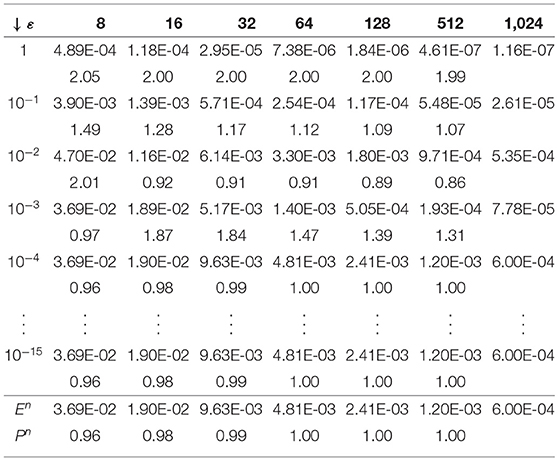
Table 1. Maximum pointwise errors and rate of convergence for Example 5.1 when n = m = {4, 8, 16, 32, 64, 128, 512, 1, 024}.

TABLE 2

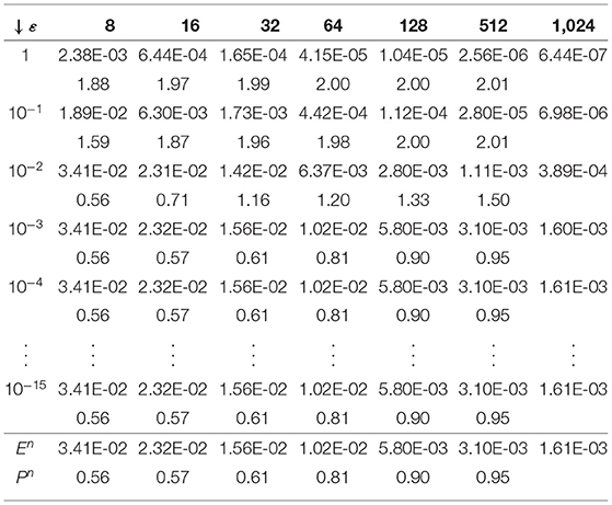
Table 2. Maximum pointwise errors and rate of convergence for Example 5.2 when n = m = {4, 8, 16, 32, 64, 128, 512, 1, 024}.

Figures 1, 2 are plots of the numerical solution of examples 5.1 and 5.2, respectively, for n = m = 32 and different values of ε. These plots exhibit the layer behavior of the numerical solution as ε approaches zero.

FIGURE 1

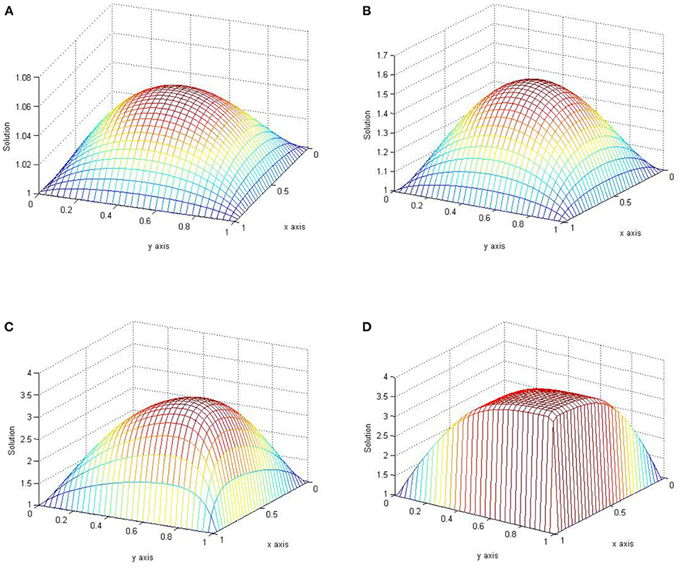
Figure 1. Plots of the approximate solution of Example 5.1 with n = m = 32. (A) ε = 1. (B) ε = 10⁻¹. (C) ε = 10⁻². (D) ε = 10⁻⁴.

FIGURE 2

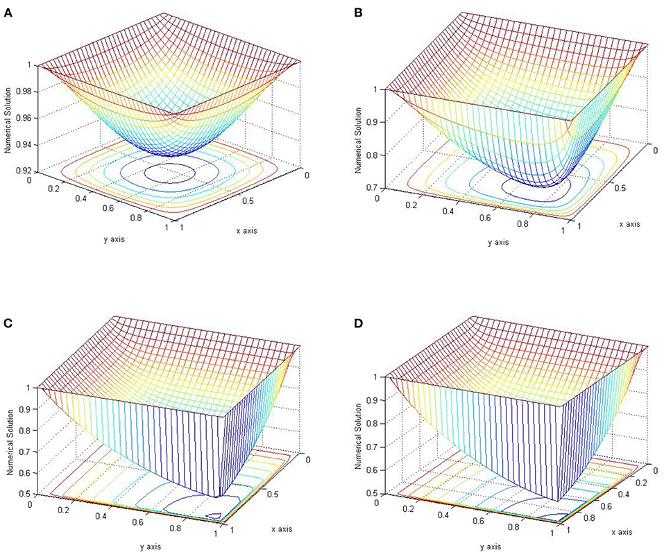
Figure 2. Plots of the approximate solution of Example 5.2 with n = m = 32. (A) ε = 1. (B) ε = 10⁻¹. (C) ε = 10⁻². (D) ε = 10⁻⁴.

We wished to compare our results with those existing in the literature however we noticed that authors that published work on this problem focused more on the number of iterations while our focus is on maximum nodal errors and rates of convergence.

6. Conclusion

In this article, we constructed a fitted operator finite difference method to solve two-dimensional semilinear singularly perturbed convection-diffusion problems. First, we converted the semilinear problems into a sequence of linear two-dimensional singularly perturbed convection-diffusion problems via the quasilinearization technique. Next, we discretized the problem using the presented non-standard numerical scheme. Then, we performed the error analysis of the method and found that it is first order uniformly convergent in both x and y variables with respect to the perturbation parameter ε. We used two test examples to illustrate the robustness of the method and to validate the theoretical findings.

Data Availability Statement

The original contributions presented in the study are included in the article/supplementary material, further inquiries can be directed to the corresponding author/s.

Author Contributions

Plan was prepared by JM and AA. Computations and analysis were done by OK under JM's supervision. Write up was done by all authors. All authors agree to be accountable for the content of this article. All authors contributed to the article and approved submitted version.

Conflict of Interest

The authors declare that the research was conducted in the absence of any commercial or financial relationships that could be construed as a potential conflict of interest.

Publisher's Note

All claims expressed in this article are solely those of the authors and do not necessarily represent those of their affiliated organizations, or those of the publisher, the editors and the reviewers. Any product that may be evaluated in this article, or claim that may be made by its manufacturer, is not guaranteed or endorsed by the publisher.

Acknowledgments

The research of JM and AA was supported by the National Research Foundation of South Africa. The authors wish to thank the reviewers for their valuable comments and suggestions that helped improve the quality of this paper.

References

1. Prandtl L. Über Flussigkeitsbewegung bei sehr kleiner Reibung. In: Proc. III Intern. Congr Math. Heildeberg (1904).

2. He X, Wang K. New finite difference methods for singularly perturbed convection-diffusion equations. Taiwanese J Math. (2018) 22:949–78. doi: 10.11650/tjm/171002

CrossRef Full Text | Google Scholar

3. Kadalbajoo MK, Patidar KC. Spline approximation method for solving self-adjoint singular perturbation problems on nonuniform grids. J Comput Anal Appl. (2003) 5:425–51. doi: 10.1155/S0161171203112094

CrossRef Full Text | Google Scholar

4. Nhan TA, Vulanovic R. The Bakhvalov mesh: a complete finite-difference analysis of two-dimensional singularly perturbed convection-diffusion problems. Num Algorith. (2021) 87:203–21. doi: 10.1007/s11075-020-00964-z

CrossRef Full Text | Google Scholar

5. Rao SCS, Chaturvedi AK. Parameter-uniform numerical method for a two-dimensional singularly perturbed convection-reaction-diffusion problem with interior and boundary layers. Math Comput Simul. (2021) 187:656–86. doi: 10.1016/j.matcom.2021.03.016

CrossRef Full Text | Google Scholar

6. Roos HG, Line T. Gradient recovery for singularly perturbed boundary value problems II: Two-dimensional convection-diffusion. Math Models Methods Appl Sci. (2001) 11:1169–79. doi: 10.1142/S0218202501001288

CrossRef Full Text | Google Scholar

7. Stynes M, Tobiska L. Necessary L2-uniform convergence conditions for difference schemes for two-dimensional convection-diffusion problems. Comput Math Appl. (1995) 29:45–53. doi: 10.1016/0898-1221(94)00237-F

CrossRef Full Text | Google Scholar

8. Alexandrov VM, Pozharskii DA, Tielking JT. Three-dimensional contact problems. Solid Mech Appl. (2002) 55:B73–4. doi: 10.1115/1.1483357

CrossRef Full Text | Google Scholar

9. Beebe NH. A Complete Bibliography of Lecture Notes in Computational Science and Engineering. (2017).

10. Gryanik V, Hartmann J. Towards a Solution of the Closure Problem for Convective Atmospheric Boundary-Layer Turbulence. Trieste: The Abdus Salam International Centre for Theoretical Physics (2017).

11. Gutkowski W, Kowalewski TA. Mechanics of the 21st century. In: Proceedings of the 21st International Congress of Theoretical and Applied Mechanics. Warsaw (2006). doi: 10.1007/1-4020-3559-4

CrossRef Full Text | Google Scholar

12. Sivertsen OI, Andrianov I. Virtual testing of mechanical systems: theories and techniques. Adv Eng. (2002) 55:B66–7. doi: 10.1115/1.1483349

CrossRef Full Text | Google Scholar

13. Ventsel E, Krauthammer T, Carrera E. Thin plates and shells: theory, analysis, applications. Appl Mech Rev. (2002) 55:B72–3. doi: 10.1115/1.1483356

CrossRef Full Text | Google Scholar

14. Sirotkin V, Tarvainen P. Parallel Schwarz methods for convection-dominated semilinear diffusion problems. J Comput Appl Math. (2002) 145:189–211. doi: 10.1016/S0377-0427(01)00575-1

CrossRef Full Text | Google Scholar

15. Boglaev I. A block monotone domain decomposition algorithm for semilinear convection-diffusion problem. J Comput Appl Math. (2005) 173:259–77. doi: 10.1016/j.cam.2004.03.011

CrossRef Full Text | Google Scholar

16. Boglaev I. Uniform convergence of monotone iterative methods for semilinear singularly perturbed problems of elliptic and parabolic types. Electron Trans Num Anal. (2005) 20:86–103.

17. Boglaev I. A monotone Schwarz algorithm for a semilinear convection-diffusion problem. J Num Math. (2004) 12:169–91. doi: 10.1515/1569395041931455

CrossRef Full Text | Google Scholar

18. Boglaev I, Duoba V. Domain decomposition for an advection-diffusion problem with parabolic layers. Appl Math Comput. (2003) 146:27–53. doi: 10.1016/S0096-3003(02)00514-3

CrossRef Full Text | Google Scholar

19. Kopteva N. How accurate is the streamline-diffusion FEM inside characteristic (boundary and interior) layers. Comput Methods Appl Mech Eng. (2004) 193:4875–89. doi: 10.1016/j.cma.2004.05.008

CrossRef Full Text | Google Scholar

20. Stynes M. Convection-diffusion-reaction problems, SDFEM/SUPG and a priori meshes. Int J Comput Sci Math. (2007) 1:412–31. doi: 10.1504/IJCSM.2007.016543

CrossRef Full Text | Google Scholar

21. Vulkov L, Zadorin AI. Two-grid algorithms for the solution of 2D semilinear singularly-perturbed convection-diffusion equations using an exponential finite difference scheme. In: AIP Conference Proceedings. American Institute of Physics (2009). p. 371–379. doi: 10.1063/1.3265351

CrossRef Full Text | Google Scholar

22. Mickens RE. Nonstandard Finite Difference Models of Differential Equations. World Scientific (1994). doi: 10.1142/2081

CrossRef Full Text | Google Scholar

23. Munyakazi JB, Patidar KC. Higher order numerical methods for singularly perturbed elliptic problems. Neural Parallel Sci Comput. (2010) 18:75–88.

24. Munyakazi JB, Patidar KC. Novel fitted operator finite difference methods for singularly perturbed elliptic convection-diffusion problems in two dimensions. J Diff Equat Appl. (2012) 18:799–813. doi: 10.1080/10236198.2010.513330

CrossRef Full Text | Google Scholar

25. Miller JJ, O'riordan E, Shishkin GI. Fitted Numerical Methods for Singular Perturbation Problems: Error Estimates in the Maximum Norm for Linear Problems in One and Two Dimensions. World Scientific (1996). doi: 10.1142/2933

CrossRef Full Text | Google Scholar

26. Kadalbajoo MK, Patidar KC. ε-uniformly convergent fitted mesh finite difference methods for general singular perturbation problems. Appl Math Comput. (2006) 179:248–66. doi: 10.1016/j.amc.2005.11.096

CrossRef Full Text | Google Scholar

27. Doolan EP, Miller JJ, Schilders WH. Uniform Numerical Methods for Problems With Initial and Boundary Layers. Eindhoven: Boole Press (1980).

Keywords: semilinear singularly perturbed problems, two-dimensional partial differential equations, fitted operator finite difference method, quasilinearization, error analysis, uniform convergence

Citation: Kehinde OO, Munyakazi JB and Appadu AR (2022) A NSFD Discretization of Two-Dimensional Singularly Perturbed Semilinear Convection-Diffusion Problems. Front. Appl. Math. Stat. 8:861276. doi: 10.3389/fams.2022.861276

Received: 24 January 2022; Accepted: 29 March 2022;
Published: 21 April 2022.

Edited by:

Dumitru Trucu, University of Dundee, United Kingdom

Reviewed by:

Yang Liu, Inner Mongolia University, China
Omar Abu Arqub, Al-Balqa Applied University, Jordan

Copyright © 2022 Kehinde, Munyakazi and Appadu. This is an open-access article distributed under the terms of the Creative Commons Attribution License (CC BY). The use, distribution or reproduction in other forums is permitted, provided the original author(s) and the copyright owner(s) are credited and that the original publication in this journal is cited, in accordance with accepted academic practice. No use, distribution or reproduction is permitted which does not comply with these terms.

*Correspondence: Justin B. Munyakazi, jmunyakazi@uwc.ac.za

^†Deceased

ORIGINAL RESEARCH article

A NSFD Discretization of Two-Dimensional Singularly Perturbed Semilinear Convection-Diffusion Problems

1. Introduction

2. Quasilinearization

3. Scheme for the Problem

4. Convergence Analysis

5. Numerical Results

6. Conclusion

Data Availability Statement

Author Contributions

Conflict of Interest

Publisher's Note

Acknowledgments

References

This article is part of the Research Topic

People also looked at