Curtailing crime dynamics: A mathematical approach
 Theophilus Kwofie
 Matthias Dogbatsey
 Stephen E. Moore
- 1School of Mathematical and Statistical Sciences, Arizona State University, Tempe, AZ, United States
- 2Department of Mathematics, The University of Alabama, Tuscaloosa, AL, United States
- 3Department of Mathematics, University of Cape Coast, Cape Coast, Ghana
- 4Africa Centre of Excellence, Regional Transport Research and Education Centre (TRECK), Kumasi, Ghana
Introduction: Crime and criminal activities have huge influences on society and societal development. The social makeup of the society has a significant impact on the propagation of crime within a population. It is a well-known reality that crime spreads across society like an infectious disease, despite the fact that there are many elements that might affect this dynamic. So, understanding crime and the factors influencing its spread are essential in formulating policies to reduce the prevalence and impacts of crime.
Methods: We formulate a deterministic mathematical model using a system of nonlinear ordinary differential equations incorporating education programs as tools to assess the population-level impact on the spread of crime. The model has a global asymptotically stable crime-free equilibrium whenever a certain criminological threshold, known as the effective reproduction number , is less than unity.
Results and discussion: The model is fitted with prison data reported from July 2021 to June 2022 by the State of Illinois in The United States. The simulations are carried out to assess the population-level impact of the widespread use of the intervention programs and the compliance rate in the State of Illinois. We hypothetically fixed the efficacy of the intervention programs at 25% while varying the compliance rate (by the general public). With no compliance, a high level of active criminal population was recorded. As the compliance rates were significantly improved, the active population level decreased. The global sensitivity analysis is performed primarily to determine the parameters with the most effect on the spread of crime in the State of Illinois. The results demonstrate that the effective community contact rate, βc, for the criminally active individuals is the main driver of crime in the State of Illinois.
1. Introduction
One of the illegal ways to undermine human civilized society is through crime. It is crucial to thoroughly handle this issue because it has existed for a very long time [1]. Crime is a significant sociological problem that has been researched extensively in the scientific literature [2]. It is difficult to provide a concrete definition of crime because every society has its own norms and values. However, what constitutes a crime is an illegal act or a perpetrator's deviant conduct, its effective punishment can be imposed by a criminal legislating institution [3, 4], and the victims of these acts. Crime mainly rises from the combination of three factors: a driven offender, a suitable target, and the absence of an able guardian [5–7]. In view of this, all crimes require opportunity but not every opportunity is followed by crime. The spread of crime usually happens as a result of coming into contact with criminally active groups of people. We may not realize the spread of crime until it becomes predominant. Consequently, it goes without saying that crime imposes costs on society.
Mathematical modeling is a powerful tool that has been employed to examine the spread of crime. One of its main goals is to understand the condition under which the spread of crime within a population will disappear or persist. For instance, the United States (U.S) government spends more on the criminal justice system than any other country. Public spending on its prison system has increased by six times the rate of government spending on higher education over the past two decades [8]. A statistical model of criminal behavior is demonstrated [10]. The role of technology in combating social crime is studied using a deterministic model [11]. Here, authors considered a deterministic compartment model and emphasized the need for technology to combat crime in society. A mathematical model considering serious and minor criminal activities are formulated and analyzed [12]. In González-Parra et al. [2], authors have studied a mathematical model by considering crime as a social epidemic. Here, authors have considered several compartments and have assumed that a judge or a police officer can also become a criminal if they come into contact with criminals. An interesting mathematical model for the dynamics of the spread of crime is formulated and analyzed [8], where authors have shown that if they relax the assumption that crime initiates only through contagion, then the crime-free equilibrium is no longer possible and the model system can tend to either lower the crime equilibrium or increase the crime equilibrium. For example, the epidemic spread of drug use has been modeled using differential equations [13–15]. In Gonzalez et al. [16], the authors constructed a model examining the dynamics of peer pressure on college-age bulimia, focusing on the effects of the intervention at two stages of the disease. The Optimal control for crime at its minimal level during festive periods such as Christmas and Valentine's day, and entertainment events, such as music awards, have also been studied and presented [17].
Introducing fear to combat crime, will reduce the expectation of a benefit, and consequently the intention to engage in crime after considering the cost. Similar research on mathematical models of crime stems from Becker's perspective of crime as a rational decision-making [18] mechanism whereby the individual compares the benefits and costs (punishment) associated with criminal activity against criminal alternatives. For example, Freedman et al. [19] developed a model that depicts that crime is concentrated in places where the possible monetary benefit from committing a crime (the probability of not being convicted due to the reward of the crime) exceeds the cost of criminal opportunity. Wang et al. [20] generalized this approach allowing for the cost of an opportunity to be heterogeneous across future criminals and depending on the level of crime in a given society and estimated the amount of group crime activity in equilibrium. Another study focused on sanction policies that reduce crime through general or specific deterrence [21, 22]. Recently, Durlauf and Nagin [23] reviewed this research and concluded that incarceration is not the optimal approach to combat crime. From several research studies, increase in prison sentence lengths are associated with weak to modest declines in crime, while micro-level studies suggest that experiencing incarceration does not seem to prevent reoffending. Their findings show that the most significant deterrent effects come from implementing tactics that increase the perceived risk of apprehension. Recidivism rates in the United States vary depending on the crime. In the case of property and drug-related offenses, the likelihood of rearrest within 3 years after release is about 70% [24]. The present study is a development of a new mathematical model for studying crime dynamics and incorporating education programs as a tool to curtailing the menace of crime and criminality in the United States of America (particularly in the State of Illinois). The model takes the form of Kermack-McKendrick, a compartmental, deterministic system of nonlinear differential equations [25]. We consider some relevant aspects of the crime dynamics, including incarceration, desistance by criminals, and how released criminals return to their previous crime life. It is worth mentioning that the model under study exhibits certain features as illustrated in Srivastav et al. [1]. The model parameterized using available crime data obtained from the Illinois Department of Corrections Prison Population Data Sets. In addition, the parameterization of the model provides an insight into the assessment of some of the education programs.
The rest of the article is organized as follows; In Section 2, we present the model formulation while the basic properties of the model are presented in Section 3. The local and global stability analysis of the Crime-free equilibrium is presented in Section 4. In Section 5, we present both the global and local sensitivity analysis of the model, and finally, we present numerical simulations and discussions in Section 6.
2. Model formulation
We present a model to assess the various education programs to curtail criminality in the State of Illinois. The total population denoted as N(t) is subdivided into mutually exclusive compartments of susceptible individuals (i.e., individuals who are at risk of becoming criminals) S(t), criminally active individuals (i.e., individuals who are actively involved in crime at any given time) C(t), criminals in prison (i.e., individuals who are caught in the act of crime and are put in prison) P(t), and reformed Individuals (i.e., individuals who have come out of prison and leading a normal life), R(t). We consider the following assumptions: (a) a homogeneously-mixed population [i.e., all individuals (both susceptible and criminals)] in the community are assumed to have an equal probability of coming into contact with one another), (b) exponentially-distributed waiting time in each criminological compartment, and (c) human demographic processes (i.e., migration, births or deaths due to causes other than the crime being modeled). Susceptible individuals join the criminal group when there is effective interaction with either criminal or prison individuals. A standard incidence
measures the force of crime, where βc and βp are community contact rates for both active criminals and criminals in prison, respectively, 0 < η ≤ 1 is the proportion of community members who observe the education programs introduced, 0 < ε ≤ 1 is the efficacy of the education programs (low values of η imply limited compliance of the intervention programs by the public, whiles values of η near unity signify widespread observance of the intervention programs). Again, values of ε close to zero imply that the intervention programs may not be a major tool to stop or reduce the spread of crime in the community.
Based on this fact (and noting the flow diagram in Figure 1), the basic model for the spread of crime dynamics in a community is given by the following deterministic system of nonlinear differential equations (where a dot represents differentiation with respect to time t):
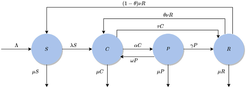
Figure 1. Flow diagram of the model (Equations 1–4).
Equation (1) describes the dynamics of the law-abiding individuals in the community S(t). The first term Λ refers to a fixed number of individuals who join the susceptible population either through migration or birth. The term (1 − θ)νR refers to the proportion of individuals who recover fully and return to the susceptible class. Equations (2) and (3) describe the dynamics within the active criminal population C(t) and prison population P(t), respectively, either through incarceration, desistance, recidivism, or proportion of individuals that return to their previous criminal life after they have been released from prison. Equation (4) highlights the modification in the reformed class R(t), which describes the movement from R(t) to C(t) and C(t) to R(t). The term ν describes the rate at which reformed individuals recover fully and return to the susceptible class S(t). We assume natural deaths occurrence in all compartments. The description of the variables and parameters are given in Tables 1, 2, respectively.
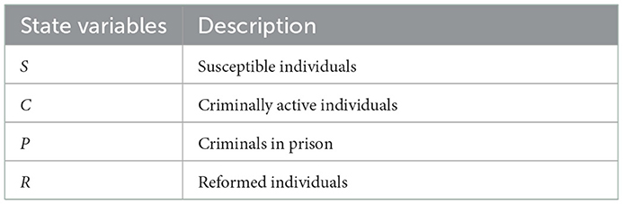
Table 1. Description of state variables of the model (Equations 1–4).

Table 2. Description of parameters of the model (Equations 1–4).
3. Basic properties of the model
Lemma 1. (Positivity) Let t > 0. In this model, if the initial conditions satisfy S(0) > 0, C(0) > 0, P(0) > 0, R(0) > 0, then for all t ∈ [0, t0], S(t), C(t), P(t), and R(t) will remain positive in for arbitrary t0.
Proof. With all the parameters used in the system being non-negative, we can thus place a lower bound on each of the equations making up the model. Thus,
By applying basic differential equations method (separation of variables), we can resolve these inequalities to produce
where Thus, for all t ∈ [0, t0], S(t), C(t), P(t), and R(t) will be positive and remain in
Lemma 2. (Boundedness) There exists an SM, CM, PM, RM > 0 such that for S(t), C(t), P(t), R(t) limsupt → ∞(S(t)) ≤ SM, limsupt → ∞(C(t)) ≤ CM, limsupt → ∞(P(t)) ≤ PM, limsupt → ∞(R(t)) ≤ RM for all t ∈ [0, t0] for arbitrary t0.
Proof. Since the model Equations (1)–(4) monitors human populations, all the associated parameters and state variables are positive, and adding the four equations of the model Equations (1)–(4) gives us
Solving Equation (9) yields
The upper bound can be found by taking the lim sup of both sides as t → ∞ to get . So N is bounded below by 0 and above by . Therefore for t ∈ [0, t0], S(t), C(t), P(t), R(t) are bounded.
The model (Equations 1–4) is biologically and mathematically well-posed in the domain
Thus, the domain, is positively invariant.
4. Stability analysis of crime-free equilibrium
4.1. Crime-free equilibrium
The model has a crime-free equilibrium (CFE), obtained by setting the right-hand sides of Equations (1)–(4) to zero, given by
with N* = S* + C* + P* + R* = Λ/μ.
4.2. Crime effective reproduction number
For infectious diseases, one of the most important threshold parameters is the basic reproduction number, denoted by which is required to determine the transmission dynamics of an infectious disease in a population. However, in criminal dynamic models, is a threshold parameter that measures the average number of new criminals produced by the relapse and interaction of the criminal population with the susceptible population [26].
The basic tool for examining epidemic thresholds in complex, structured models is the so-called next-generation matrix [27]. We use the next-generation method to compute the crime effective reproduction number for our model. Here, we assumed that each function is at least twice continuously differentiable in each variable
where f is the rate of appearance of a new crime in a compartment and v is the rate of transfer of individuals into and out of a compartment. We linearized the two expressions earlier with respect to C and P to obtain
since S* = N*. The effective or control reproduction number, denoted by , is then given by where ρ(·) denotes the spectral radius (dominant eigenvalue). It follows that
where
Thus by expressing in terms of , we obtain
In the absence of intervention strategies (i.e., ε = 0 = η), the effective reproduction number is given by
where
Remark 1. The expression ψ represents the proportion of active criminals incarcerated and reverted back to be criminals or the likelihood that a criminal will return to being a criminal again. The terms and are the duration of stay in compartments C and P, respectively. The expression is the proportion of active criminals that are imprisoned or the probability that a criminal will be sent to prison, and is the proportion of prisoners that are released and go back into criminality.
is the number of individuals a criminal activist can influence during the period of successful criminal behavior where intervention programs are introduced into the community. The effective reproduction number of the model (Equations 1–4) is expressed as the sum of two constituents reproduction numbers, namely the average number of new crimes generated by a typical active criminal in a community, denoted by , and the average number of crimes generated by a typical criminal in prison, denoted by
4.3. Local stability analysis of crime-free equilibrium
Theorem 4.1. The CFE () of the model (Equations 1–4) is locally asymptotically stable (LAS) if . If , the crime rises to a peak and then eventually declines to zero.
Proof. The local stability of the CFE () is determined by using the eigenvalues of the Jacobian matrix at , given by
where K1 = (μ + α + τ), K2 = (μ + γ + ω), and K3 = (μ + ν). It is easy to see that the first negative eigenvalue is λ1 = − μ. The remaining eigenvalues are obtained below:
The characteristic polynomial of the aforementioned matrix J⋆ is given by
where
Applying the Routh-Hurwitz criterion [28], it is clear that a1 > 0 if K1 + K2 + K3 > βc(1 − ε η). It should be emphasized that makes a3 > 0. Furthermore, if , then a3 < 0. The condition , makes
The two inequalities (Equations 13–14) imply that a2 > 0. Finally, we need to show that a1a2 > a3. After algebraic manipulations, we have that a1a2 > a3. Thus, the crime-free equilibrium of the model (Equations 1–4) is locally asymptotically stable whenever otherwise unstable.
The criminological implication of Theorem 4.1 is that a small influx of active criminal individuals in the community will not generate an outbreak of crime in the community if . That is, the spread of crime rapidly dies out (when ) if the initial number of active criminal individuals in the community are in the basin of attraction of the CFE (). For instance, when , one active criminal in the community will, on average, influence two other individuals during the duration of his/her successful criminal behavior. Hence, in this case, the crime will be spreading exponentially until intervention strategies are implemented in the community and/or a certain proportion of the public is educated. In this article, since intervention measures are put in place to help stop or reduce the spread of crime, the rate at which crime spreads will be minimized. In order for crime elimination to be independent of the initial size of the sub-populations of the model, it is necessary to show that the crime-free equilibrium () is globally asymptotically stable.
4.4. Global asymptotic stability of the crime-free equilibrium
The global asymptotic stability of the crime-free equilibrium of the model (Equations 1–4) can be established for the special case, that is in the absence of re-committing the crime (i.e., θ = 0).
Theorem 4.2. Consider the special case of the model (Equations 1–4) in the absence of re-committing the crime (i.e., θ = 0), the crime-free equilibrium () of the model (Equations 1–4) is globally asymptotically stable in whenever .
The proof of Theorem 4.2 is based on using a comparison theorem [29].
Proof. Consider the special case of the model (Equations 1–4) in the absence of re-committing the crime. Let us assume that . The equations for the crime compartments for the special case of the model (Equations 1–4) can be re-written in terms of the next generation matrices ( and ) as follows:
where (with S* and N* as defined in Section 11),
and
Since S ≤ N for all t > 0 in , it follows that the matrix , defined in Equation (16), is non-negative. Hence, the Equation (15) can be re-written in terms of the following inequality:
If , this implies that all eigenvalues of the next generation matrix are negative. Equivalently, we can claim that is a stable matrix [27]. Thus, it can be concluded that the linearized differential inequality system (Equation 17) is stable whenever . Hence, it follows from aforementioned analysis that
Eventually after substituting C(t) = P(t) = 0 into the differential equations for the rate of change of the R(t) and S(t) compartments shows that
Hence, we can finally claim that the CFE (given in Section 11) for the special case of the model (Equations 1–4) (with θ = 0) is globally asymptotically stable in whenever .
The criminological implication of Theorem 4.2 shows that, for the special case of the model (Equations 1–4) with θ = 0, the overall crime can be eliminated from the community if is brought to and maintained to a value less than unity.
5. Sensitivity analysis
We use sensitivity analysis to determine the robustness of model predictions to parameter values since there usually are errors in data collection and presumed parameter values [30]. Sensitivity indices also enable us to quantify the change in the state variables that results from changes in the parameters [9]. Sensitivity analysis is used to discover parameters that have a high impact on the crime reproductive number and should be targeted by intervention strategies. We define the normalized forward sensitivity index (NFSI) of the effective crime reproduction number as the relative change in occasioned by the relative change in each of the parameters. The normalized forward sensitivity index of a variable to a parameter is the ratio of the relative change in the variable to the relative change in the parameter. Since the effective crime reproduction number is differentiable with respect to all the parameters, we define the sensitivity index as follows:
Definition 1. For an effective crime reproduction number, , differentiable with respect to the parameter q, the normalized forward sensitivity index (NFSI) is defined as
Using this definition, we estimate the sensitivity indices of the parameters of the effective crime reproduction number as follows:
The final sign of the last index is dependent on the value of the numerator. It is easily verifiable that all the index values are less than 1. Since the effective crime reproductive number plays a critical role in the spread of crime, it is important to identify the most effective approach in bringing down our . To this end, we perform numerical simulations using the baseline parameter values given in Tables 3, 4 to identify which parameters are sensitive to the effective reproductive number.
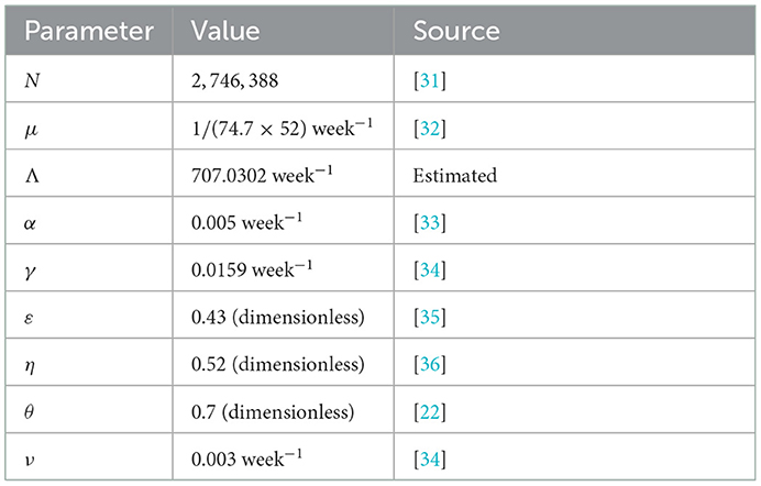
Table 3. Baseline values of the fixed parameters of the model (Equations 1–4).
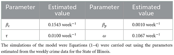
Table 4. Baseline values of fitted (estimated) parameters of the model (Equations 1–4), obtained by fitting the model with the weekly crime data for Illinois for the period July 1st, 2021 to June 30th, 2022.
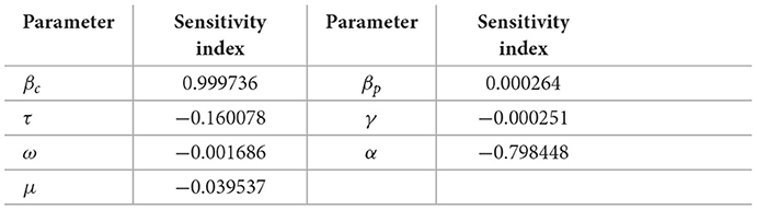
We observe that community contact rate for active criminals βc has nearly one to one corresponding relationship with the crime reproductive number such that a 10% change in βc results in a 9.9% change in So the crime reproductive number is most sensitive to βc. The crime reproductive number also has a direct proportional relationship with the parameter βp. However, the effect is much lower, a 100% change in βp only leads to 0.26% change in the crime reproductive number. The crime reproductive number has an inverse proportional relationship with parameters τ, ω, γ, α, μ; an increase in any of them will bring about a decrease in crime reproductive number
5.1. Data fitting and parameter estimation
In this section, we have fitted the observed weekly cumulative crime data for Illinois from the period of 1 July 2021 to 30 June 2022 [37]. The time series illustration of the least squares fit of the model (Equations 1–4) is depicted in Figure 2, showing the model estimation (i.e., blue curve which is plotted for the criminals in prisons as formulated in Equation 3) represents the cumulative weekly crimes compared to the observed cumulative weekly crime data (i.e., red dots) for the aforementioned time period.
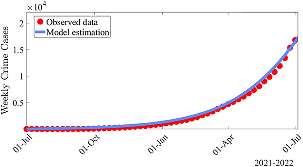
Figure 2. Data fitting of the model (Equations 1–4) using weekly crime data for Illinois from 1 July 2021 to 30 June 2022. The simulations of the model (Equations 1–4) carried out using the parameters estimated from the weekly crime data for the Illinois. The values of the fixed and fitted parameters used for the purpose of the data fitting and parameter estimation are shown in Tables 3, 4, respectively.
The developed model has a total of 13 different parameters, out of which 8 parameters are known from the existing literature which is shown in Table 3. We have calculated the daily recruitment rate (Λ) as a product of the total population (N) of Illinois, which is based on the projections of the latest U.S. census [31] and the weekly natural mortality rate (µ) The developed model was fitted using a standard nonlinear least squares approach, which involved using the inbuilt Matlab R2022a optimizer function “lsqcurvefit,” which will be used to obtain the best values of the remaining four unknown parameters. SSE minimizes the sum of the squared differences between each observed cumulative crime data points and the corresponding cumulative crime points obtained from the model (Equations 1–4). The estimated values of the unknown parameters which are obtained from the fitting are shown in Table 4. The effective reproduction number for the set of the fixed and fitted parameters for the model (Equations 1–4) is .
6. Numerical simulations and discussions
To demonstrate some of the various theoretical results contained in this paper, the model (Equations 1–3) is simulated using the baseline values shown in Table 3 (unless otherwise stated), to assess the population-level impact of the interventions programs (in a form of education) against crime level in Illinois. It is worth noting that throughout the simulations, Matlab R 2022a was used, and the initial conditions considered are S(0) = 2, 742, 386, C(0) = 3, 950, P(0) = 2, and R(0) = 50. We also simulated the model (Equations 1–3) using the calibrated parameters in Table 4, coupled with other estimated parameters in Table 3 to assess the population-level impact of mitigation strategies. First of all, we simulated the model to assess the population-level impact of the incarceration on the active criminal population. The population-level impact of incarceration is measured by the reduction of the active criminal population.
One thing that is important in the fight against crime is the rate of uptake into correctional facilities of criminals. We varied the rate of uptake into rehabilitation (α) and we found that as the rate of incarceration increases, the number of criminals in the population reduces as a result. Thus, the more criminals are incarcerated and put in rehabilitation programs, the more crime reduces. This can be seen in Figure 3. This observation is consistent with the conclusion from similar studies done by Nyabadza et al. [9] and Berenji et al. [38]. Liedka et al. [39] observed that there exists a negative relationship between prison(incarceration) and crime. Rose et al. [40] observed that within 3 years of incarceration, the risk of committing new assault crimes, property crimes, and drug crimes reduced by 38%, 24%, and 30%, respectively.
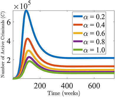
Figure 3. Effect of varying the incarceration rate α on the criminal population. Simulation displaying the active criminal population, as a function of time. The values of the parameters are used from Tables 3, 4 with the values of α being varied.
In Figure 4, the simulations are carried out to assess the population-level impact of the widespread use of the intervention programs and the compliance rate in the Illinois. This Figure shows a marked decrease in the active criminal population with varying efficacy and compliance rates. For (a), we hypothetically fixed the efficacy of the intervention programs at 25% while varying the compliance rate (by the general public). With no compliance, a high level of the active criminal population (approximately 2,020,650) was recorded. As the compliance rates were significantly improved, the active population level decreased. For (b), we hypothetically improved the efficacy rate by fixing it at 50% and realized that increasing the compliance rates by 25% dramatically flattens the active criminal population curves. However, with such an efficacy level coupled with the varying compliance rates, the crime level in the community may still persist. Even though the use of intervention programs with low-level of efficacy rates may not lead to the elimination of crime in the community, they have the potential of reducing the burden of crime in the community (Figure 4B). An interesting observation was made when the efficacy and compliance were 75 and 25%, respectively. The burden of active criminal populations reduces, almost leading to the eventual eradication of crime in the population. In order to effectively measure the impact of the intervention programs, it is imperative to consider further increasing the efficacy levels while varying the compliance rates. For a case where 100% of the populace in Illinois complies with the intervention programs with a low-efficacy rate of 50%, the number of active criminals in the community will be reduced. As it is clear that it will be impossible to have everyone comply with the education programs. However, with the right set of strategies, many of the populace may understand the message and eventually comply with it.
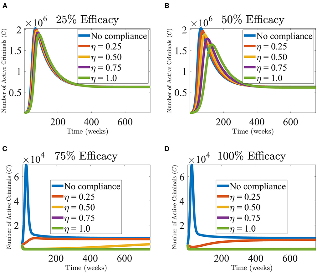
Figure 4. Effect of intervention programs in the Illinois community. The simulation of the model (Equations 1–3), showing the weekly crime levels, as a function of time, for the assessment of the impact of the intervention programs (ε) and the compliance rate (η); (A) 25% efficacy of intervention programs, (B) 50% efficacy of intervention programs, (C) 75% efficacy of intervention programs, and (D) 100% efficacy of intervention programs for Illinois. Allowing for the assessment of the combined effect of the intervention strategies and how the masses comply with the policies. The improvement in the intervention strategies and compliance rate are measured in terms of the percentage reduction of crime levels in Illinois. The other parameter values used are given in Tables 3, 4.
Authors in Zitko [41] made a comparison of state-level education data and crime and incarceration rates, and they realized that states that have focused the most on education (in general, financial support) tend to have lower rates of violent crime and incarceration. Although education cannot be seen as a “cures all” or a panacea that will ensure declines in criminal behavior or crime rates, research indicates that increased spending on high-quality education can have a favorable impact on public safety. Many trends have been supported by contemporary research that has examined possible connections between education and criminal behavior. Both the idea that people with learning difficulties are more likely to engage in violent behavior and the idea that education levels (both greater and lower) are important in the manifestation of criminal behavior have empirical backing. Numerous criminologists have examined the connection between intelligence and crime in their writings, frequently discovering an inverse link between the two. In other words, criminologists have discovered that those with lower IQs are more likely to commit a crime than people with higher IQs [42]. However, James Oleson's “Criminal Genius” sheds light on the offenses–drawn from self-reports and interviews–committed by high-IQ individuals, a group understudied in the field of criminology [42].
6.1. Global sensitivity analysis
The model (Equations 1–3) has 12 parameters and the purpose of the sensitivity analysis is to measure the impact of the sensitivities of the parameters on the outcome of the numerical simulation results (with respect to a particular response function). The standard uncertainty and sensitivity analysis, using the Latin Hypercube Sampling technique and partial rank correlation coefficients (PRCCs) were applied to ascertain the sensitivities of the parameters against the crime compartment which is a function of time (as a response function) [43]. Other response functions, such as the crime effective reproduction number (), could have been used to measure such sensitivities of the parameters. To do the sensitivity analysis, each model parameter's range (lower and upper bound) and distribution must first be defined, followed by the division of each range into 1,000 equal sub-intervals. A 1,000 × 12 matrix is created by randomly selecting parameter sets from this space without replacing them [44, 45]. The values of the response function (crime compartment which is a function of time) are obtained for each row of this matrix, and then PRCCs are computed to analyze the contributions of uncertainty and variability in specific parameters to uncertainty and variability in the response function. High PRCC values near 1 or -1 are seen as significantly correlated with the response function, whereas low PRCC values are regarded as negatively (or positively) correlated with the response function. We assume, for simplicity, that each of the 12 parameters of the model (Equations 1–3) obeys a uniform distribution, and the range for each parameter is obtained by taking 20% to the left, and then 20% to the right, of its baseline value (given in Tables 3, 4) [43].
In Figure 5, the parameters that have a great impact on the response variable are the community effective contact rate for criminally active individuals (βc), the rate of desistance by criminals (τ), and the recidivism rate (ω). This explains that the effective community contact rate for criminally active individuals is the main driver of crime in our society.
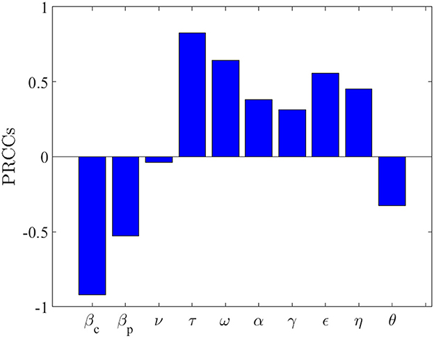
Figure 5. Partial rank correlation coefficients (PRCCs) showing the effects of the model parameters on the response variable (which in our case is the crime population as a function of time). The baseline values of the parameters used are given in Tables 3, 4.
We depict the contour plots of the effective reproduction number as a function of the intervention programs (ϵ) and the compliance rate (η) at steady-state in Figure 6. As expected, the increment in the efficacy of the intervention programs along with the increment in the proportion of community members who observe the education program (i.e., the compliance rate) has a significant impact on the reduction of . Furthermore, it is notable from Figure 6 that to keep and maintain to a value less than unity, we need to keep the intervention programs and the compliance rate above 95%. On the contrary, if due to any reasons, the intervention programs and the compliance rate both drop down drastically to 20% or even much lower than it, so for this scenario, we could observe that the value of increases dramatically to 14 or even above. Overall, our study shows that to effectively control crime in the community, it is necessary and sufficient to keep the efficacy of the intervention programs and the compliance rate of the education programs above 95%. Thus, a strategy that emphasizes the significant increments in ϵ and η would notably enhance the prospects of crime elimination in the state of Illinois.
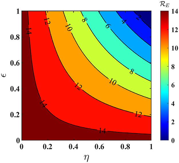
Figure 6. The contour plot of the effective (or control) reproduction number , as a function of the intervention programs (ϵ) and the compliance rate (η). The other parameter values used for the contour plot are given in Tables 3, 4, respectively.
7. Conclusion
In this paper, we developed a mathematical model that incorporates programs in curtailing crime dynamics. The deterministic model was fitted with crime data from Illinois [37] in the United States (U.S.) by means of a least squares method. We present both local and global asymptotic analysis for the crime free equilibrium. We observed globally asymptotically stable crime-free equilibrium whenever the effective crime reproduction number is less than one, i.e., By using the partial rank correlation coefficients (PRCCs) method, we are able to estimate the parameters that have a significant influence on the model. We observed that the community effective contact rate for criminally active individuals (βc), the rate of desistance by criminals (τ), and the recidivism rate (ω) tend to have a great impact on the spread of crime, see, Figure 5. The numerical simulation shows that with an efficacy level of 75% with varying compliance levels (0 − 100%), the burden of crime will be reduced drastically.
Data availability statement
Publicly available datasets were analyzed in this study. This data can be found at: https://www2.illinois.gov/idoc/reportsandstatistics/Pages/Prison-Population-Data-Sets.aspx.
Author contributions
TK, MD, and SM: conceptualization, methodology, formal analysis, writing—original draft, writing—review, and editing. All authors contributed to the article and approved the submitted version.
Funding
SM was supported by a grant from UNESCO-TWAS and the Swedish International Development Cooperation Agency (SIDA).
Acknowledgments
Thanks to the reviewers whose comments helped improve the article.
Conflict of interest
The authors declare that the research was conducted in the absence of any commercial or financial relationships that could be construed as a potential conflict of interest.
Publisher's note
All claims expressed in this article are solely those of the authors and do not necessarily represent those of their affiliated organizations, or those of the publisher, the editors and the reviewers. Any product that may be evaluated in this article, or claim that may be made by its manufacturer, is not guaranteed or endorsed by the publisher.
Author disclaimer
The views expressed herein do not necessarily represent those of UNESCO-TWAS, SIDA or its Board of Governor.
References
1. Srivastav AK, Ghosh M, Chandra P. Modeling dynamics of the spread of crime in a society. Stochastic Anal Appl. (2019) 37:991–1011. doi: 10.1080/07362994.2019.1636658
2. González-Parra G, Chen-Charpentier B, Kojouharov HV. Mathematical modeling of crime as a social epidemic. J Interdisc Math. (2018) 21:623–43. doi: 10.1080/09720502.2015.1132574
3. Block CR, Block RL. Crime definition, crime measurement, and victim surveys. J Soc Issues. (1984) 40:137–59. doi: 10.1111/j.1540-4560.1984.tb01086.x
4. Garside R. Criminal justice since 2010. What happened, and why? Richard Garside considers the divergent policy developments within the three jurisdictions. Crim Justice Matters. (2015) 100:4–8. doi: 10.1080/0268117X.2015.1061331
5. Ajayi J, Adefolaju T. Crime prevention and the emergence of self-help security outfits in South-western Nigeria. Int J Humanities Soc Sci. (2013) 3:287–99.
6. Ayodele JO. Crime-reporting practices among market women in oyo, nigeria. SAGE Open. (2015) 5:940. doi: 10.1177/2158244015579940
7. Squires P, Grimshaw R, Solomon E. (2008). English ‘Gun crime': A Review of Evidence and Policy. Whose Justice? (Centre for Crime and Justice Studies). © Centre for Crime and Justice Studies (2008).
8. McMillon D, Simon CP, Morenoff J. Modeling the underlying dynamics of the spread of crime. PLoS ONE. (2014) 9:e88923. doi: 10.1371/journal.pone.0088923
9. Nyabadza F, Ogbogbo C, Mushanyu J. Modelling the role of correctional services on gangs: insights through a mathematical model. R Soc Open Sci. (2017) 4:170511. doi: 10.1098/rsos.170511
10. Pasour V, Tita G, Brantingham P, Bertozzi A, Short M, D'Orsogna M, et al. A statistical model of crime behavior. Math Methods Appl Sci. (2008) 107:1249–67. doi: 10.1142/S0218202508003029
11. Shukla JB, Goyal A, Agrawal K, Kushwah H, Shukla A. Role of technology in combating social crimes: a modeling study. Eur J Appl Math. (2013) 24:501–14. doi: 10.1017/S0956792513000065
12. Lacey A, Tsardakas M. A mathematical model of serious and minor criminal activity. Eur J Appl Math. (2016) 1:1–19. doi: 10.1017/S0956792516000139
13. Behrens D, Caulkins J, Tragler G, Haunschmied J, Feichtinger G. A dynamic model of drug initiation: implications for treatment and drug control. Math Biosci. (1999) 159:1–20. doi: 10.1016/S0025-5564(99)00016-4
14. Song B, Castillo-Garsow M, Rios-Soto K, Mejran M, Henso L, Castillo-Chávez C. Raves, clubs and ecstasy: the impact of peer pressure. Math Biosci Eng. (2006) 3:249. doi: 10.3934/mbe.2006.3.249
15. White E, Comiskey C. Heroin epidemics, treatment and ODE modelling. Math Biosci. (2007) 208:312–24. doi: 10.1016/j.mbs.2006.10.008
16. Gonzalez B, Huerta-Sánchez E, Ortiz-Nieves A, Vázquez-Alvarez T, Kribs-Zaleta C. Am I too fat? Bulimia as an epidemic. J Math Psychol. (2003) 47:515–26. doi: 10.1016/j.jmp.2003.08.002
17. Ohene Opoku NKD, Bader G, Fiatsonu E. Controlling crime with its associated cost during festive periods using mathematical techniques. Chaos Solitons Fractals. (2021) 145:110801. doi: 10.1016/j.chaos.2021.110801
18. Becker GS. Crime and punishment: an economic approach. J Political Econ. (1968) 76:169–217. doi: 10.1086/259394
19. Freeman S, Grogger J, Sonstelie J. The spatial concentration of crime. J Urban Econ. (1996) 40:216–31. doi: 10.1006/juec.1996.0030
20. Wang SJ, Batta R, Rump C. Stability of a crime level equilibrium. Soc Econ Plann Sci. (2005) 39:229–44. doi: 10.1016/j.seps.2004.01.001
21. Nagin DS. Deterrence in the twenty-first century. Crime Justice. (2013) 42:199–263. doi: 10.1086/670398
22. Nagin D. Deterrence: a review of the evidence by a criminologist for economists. Ann Rev Econ. (2012) 5:1310. doi: 10.1146/annurev-economics-072412-131310
23. Durlauf S, Nagin D. Overview of imprisonment and crime: can both be reduced?”. Criminol Public Policy. (2011) 10:9–12. doi: 10.1111/j.1745-9133.2010.00681.x
24. Nagin DS, Cullen FT, Jonson CL. Imprisonment and reoffending. Crime Justice. (2009) 38:115–200. doi: 10.1086/599202
25. Kermack WO, McKendrick AG. A contribution to the mathematical theory of epidemics. Proc R Soc Lond A. (1927) 115:700–21. doi: 10.1098/rspa.1927.0118
26. van den Driessche P, Watmough J. Further Notes on the Basic Reproduction Number. Berlin; Heidelberg: Springer Berlin Heidelberg (2008).
27. Van den Driessche P, Watmough J. Reproduction numbers and sub-threshold endemic equilibria for compartmental models of disease transmission. Math Biosci. (2002) 180:29–48. doi: 10.1016/S0025-5564(02)00108-6
29. Lakshmikantham V, Leela S, Martynyuk AA. Stability Analysis of Nonlinear Systems. Springer (1989).
30. Chitnis N, Hyman JM, Cushing JM. Determining important parameters in the spread of malaria through the sensitivity analysis of a mathematical model. Bull Math Biol. (2008) 70:1272–96. doi: 10.1007/s11538-008-9299-0
31. Chicago IP. 020 US Census Updated (2022). Available online at: https://worldpopulationreview.com/us-cities/chicago-il-population (accessed August 11, 2022).
32. Kekatos M. Life Expectancy in Chicago Declined During 1st Year of COVID Pandemic, Especially for People of Color (2022). Available online at: https://abcnews.go.com/Health/life-expectancy-chicago-declined-1st-year-covid-pandemic/story?id=84314520 (accessed August 11, 2022).
33. Initiative PP. Illinois Incarceration Rate (2022). Available online at: https://www.prisonpolicy.org/profiles/IL.html (accessed August 11, 2022).
34. Chicago L. A Plan to Help Returning Citizens Succeed in Chicago (2022). Available online at: http://www.lightfootforchicago.com/wp-content/uploads/2019/02/LL_ReturningCitizens_policy.pdf (accessed August 11, 2022).
35. Zitko PA. The Efficacy of Correctional Education (2022). Available online at: http://www.zitko.net/efficacy-of-prison-education (accessed August 11, 2022).
36. Harlow CW. Education Correctional Populations (2022). Available online at: http://bjs.ojp.gov/content/pub/pdf/ecp.pdf (accessed August 11, 2022).
37. Illinois State U. Prison Population Data Sets-Report (2022). Available online at: https://www2.illinois.gov/idoc/reportsandstatistics/Pages/Prison-Population-Data-Sets.aspx
38. Berenji B, Chou T, D'Orsogna MR. Recidivism and rehabilitation of criminal offenders: a carrot and stick evolutionary game. PLoS ONE. (2014) 9:e85531. doi: 10.1371/journal.pone.0085531
39. Liedka RV, Piehl AM, Useem B. The crime-control effect of incarceration: does scale matter? Criminol Public Policy. (2006) 5:245–76. doi: 10.1111/j.1745-9133.2006.00376.x
41. Education and Crime (2022). Available online at: https://criminal-justice.iresearchnet.com/crime/education-and-crime/4/
42. Oleson JC. Criminal Genius: A Portrait of High-IQ Offenders. Berkeley, CA: University of California Press (2016).
43. Gumel AB, Iboi EA, Ngonghala CN, Elbasha EH. A primer on using mathematics to understand COVID-19 dynamics: modeling, analysis and simulations. Infect Dis Model. (2021) 6:148–68. doi: 10.1016/j.idm.2020.11.005
44. Marino S, Hogue IB, Ray CJ, Kirschner DE. A methodology for performing global uncertainty and sensitivity analysis in systems biology. J Theor Biol. (2008) 254:178–96. doi: 10.1016/j.jtbi.2008.04.011
Keywords: crime dynamics, effective reproduction number, stability analysis, sensitivity analysis, USA
Citation: Kwofie T, Dogbatsey M and Moore SE (2023) Curtailing crime dynamics: A mathematical approach. Front. Appl. Math. Stat. 8:1086745. doi: 10.3389/fams.2022.1086745
Received: 01 November 2022; Accepted: 28 December 2022;
Published: 24 January 2023.
Edited by:
Ramoshweu Solomon Lebelo, Vaal University of Technology, South AfricaReviewed by:
Mahmoud Abdel-Aty, Sohag University, EgyptAnastasiia Panchuk, Institute of Mathematics (NAN Ukraine), Ukraine
Copyright © 2023 Kwofie, Dogbatsey and Moore. This is an open-access article distributed under the terms of the Creative Commons Attribution License (CC BY). The use, distribution or reproduction in other forums is permitted, provided the original author(s) and the copyright owner(s) are credited and that the original publication in this journal is cited, in accordance with accepted academic practice. No use, distribution or reproduction is permitted which does not comply with these terms.
*Correspondence: Stephen E. Moore,  stephen.moore@ucc.edu.gh