Toward a Unification of System-Theoretical Principles in Biology and Ecology—The Stochastic Lyapunov Matrix Equation and Its Inverse Application

Weckwerth, Wolfram

doi:10.3389/fams.2019.00029

HYPOTHESIS AND THEORY article

Front. Appl. Math. Stat., 05 July 2019
Sec. Systems Biology Archive
Volume 5 - 2019 | https://doi.org/10.3389/fams.2019.00029

Toward a Unification of System-Theoretical Principles in Biology and Ecology—The Stochastic Lyapunov Matrix Equation and Its Inverse Application

Wolfram Weckwerth^1,2^*

¹Division Molecular Systems Biology, Department of Ecogenomics and Systems Biology, University of Vienna, Vienna, Austria
²Vienna Metabolomics Center (VIME), University of Vienna, Vienna, Austria

System theory has its roots in mathematical formalisms developed by mathematicians and physicists, such as Leibniz, Euler, and Newton, and applied by congenial chemists and biologists such as Lotka and Bertalanffy. In these approaches, the dynamical system—may it be either single organisms or populations of organisms in their ecosystems—is defined and formally translated into an interaction matrix and first-order ordinary differential equations (ODEs) which are then solved. This provides the background for the quantitative analysis of any linear to non-linear system. In his inspiring article “Can a biologist fix a radio?,” Lazebnik made the differences very clear between a “guilt by association” hypothesis of a modern biologist vs. a Signal–Input–Output (SIO) model of an electrical engineer. The drawback of this “Gedankenexperiment” is that two rather different approaches are compared—a forward model predictive control approach in the case of the SIO model by an engineer and an inverse or reverse approach by the biologist or ecologist. Biological and ecological systems are much too complex to estimate all the underlying ODE's, parameter and input signals that generate a probability distribution. Thus, the combination of inverse data-driven modeling and stochastic simulation is a key process for understanding the control of a biological or ecological system. The challenge of the next decades of systems biology is to link these approaches more systematically. Over the last years, we have developed a hybrid modeling approach based on the stochastic Lyapunov matrix equation for the analysis of genome-scale molecular data. This workflow connects forward and inverse strategies such as the genome-scale-based metabolic reconstruction of an organism and the calculation of dynamics around a quasi-steady state using statistical features of large-scale multiomics data. Ultimately, this workflow is linked to physiology and phenotype (the output) to unambiguously define the genotype–environment–phenotype relationship. This system-theoretical formalism establishes the generic analysis of the genotype–environment–phenotype relationship to finally result in predictability of organismal function in the environmental context. The approach is based on fundamental mathematical control theory for the analysis of dynamical systems using eigenvalues and matrix algebra, stochastic differential equations (SDEs), and Langevin- and Fokker–Planck-type equations eventually leading to the continuous stochastic Lyapunov matrix equation. The stochastic Lyapunov matrix equation is also a fundamental approach for the analysis and control of artificial intelligence systems in model predictive control and thus opens up completely new perspectives for the integration of systems engineering and systems biology. Furthermore, similar mathematical formalisms—using a community matrix instead of a stoichiometric matrix of a metabolic network—were also conceptually developed and applied by ecologists such as Levins and May in the analysis of stability and complexity of model ecosystems. Thus, the generalization of this hybrid forward–inverse approach spans from biology to ecology and promises to be a systematic iterative process that finally leads to functional units able to explain living systems up to their interaction in complex ecosystems.

Reflections on Historical Developments

Systems biology is a modern development in biology integrating genome-scale molecular analysis, e.g., metabolomics, proteomics, and transcriptomics, with computer-based mathematical and statistical modeling of metabolism and regulation. The aim is, on the one hand, to derive causal mechanisms from molecule to organism and, on the other, to establish quantitative models for the prediction of phenotypes from genotypes. Ultimately, systems biology aims for a universal genotype–environment–phenotype equation, especially in the era of genome sequencing. These ideas were already developed a long time ago in the work of Ludwig von Bertalanffy, e.g., in the book Vom Molekül zur Organismenwelt [1]. In one of his most important pioneering publications, Der Organismus als physikalisches System betrachtet, Bertalanffy describes already in 1940 the mathematical modeling of an open biochemical system and derives analytical rules for self-organization [2]. In the following years, he realized that these rules can be generalized and applied to all non-linear complex systems in biology, ecology, economy, sociology, etc., and called this “General System Theory” [3]. The technical limitations of Bertalanffy and his time were almost insurmountable in all aspects of the molecular and mathematical analysis of a complex biochemical organismal system. The system that he defined in 1940 consisted of four (five) components with four differential equations. This system could be solved analytically and principles of self-regulation and -organization were demonstrated [2].

Now, where are we standing, almost 80 years later, when we talk about an organism, microorganisms, plants, animals, or human? After the elucidation of the molecular principles of inheritance and information storage in the 1950s [4], the definition of the central dogma of molecular biology by Francis Crick [5], and the not foreseeable rapid development of next-generation sequencing after the first release of a human and a higher plant genome sequence [6–8], a day-by-day increasing remarkable number of genome sequencing projects—last estimates are 300,000—is available. All these developments could not be anticipated by Bertalanffy and colleagues and open up a completely new avenue of thinking. Using a genome sequence, it is possible to reconstruct the genome-scale metabolic network comprising typically more than 3,000 reactions in a plant, animal, human, and other systems [9–16]. To translate this into Bertalanffy's world and a system-theoretical approach, respectively, it is necessary to create more than 3,000 coupled differential equations. They form an interactive, dynamic, and causal metabolic network of the organism. These complex systemic networks were not solvable at Bertalanffy's time, but nowadays, it is possible to numerically approximate solutions [16]. Paralleling genome sequencing, further technology platforms evolved in the last decades, which are far away from Bertalanffy's imaginations such as genome-scale RNAseq, proteomics, and metabolomics [17]. Those bioanalytical approaches follow Francis Crick's idea of molecular information flow and resolve highly complex mixtures of transcripts, proteins, and metabolites. To reveal their dynamic relations and complex network topologies a plethora of uni- and multivariate statistical methods are applied to allow data integration and interpretation [18–21]. In a last step, the statistical models are linked to mathematical models of the underlying causal system, e.g., ordinary and partial differential equations as well as stochasticity [22]. The resulting causal interaction networks and the corresponding dynamics eventually elucidate molecular and phenotypic traits and thereby close the circle to Bertalanffy's imaginations to describe an organism from molecule to organism as proposed in 1944 [1].

Genome-scale Molecular Analysis—A PANOMICS Platform Combined With Data-Driven Modeling

In the following, I will introduce techniques for genome-scale molecular analysis as well as mathematical and statistical hybrid modeling as fundamental requirements to fulfill this proposed cycle of understanding the dynamics of an organism. The comprehensive analysis of organisms, microbes, plants, fungi, animals, and human begins nowadays with genome sequencing using “next-generation sequencing” technologies [12]. On the basis of a full genome sequence and following the information flow from genome to transcriptome to proteome to metabolome, subsequent genome-scale molecular techniques such as transcriptomics (RNAseq), proteomics, and metabolomics—a PANOMICS strategy—are employed to reveal a complete picture of molecular dynamics of the respective organism (Figure 1). In parallel, comprehensive genome-scale metabolic reconstructions are derived from the genome sequence by comparing orthologous genes and their functions by database search, e.g., using UNIPROT with annotated protein sequences and functions of up to 160 million predicted proteins [15, 23]. A comprehensive discussion of all these initial steps up to the PANOMICS platform to investigate an organism is described in a recent publication entitled the “unpredictability of metabolism from genome sequences” [12]. This obviously contrasting title comes from the fact that a genome-scale metabolic reconstruction does not reflect any dynamics or plasticity of metabolism. In other words, the phenotypic plasticity of an organism that is the result of the interaction with its environment cannot be derived from the genome sequence alone, at least not at this stage of biological and biochemical knowledge. A hope is, of course, to apply system-theoretical ideas and, thus, systems biology to this problem of functional genome annotation to finally give a causal–functional interpretation of a newly sequenced genome up to its molecular and phenotypical dynamics in relation to its environment. It is further obvious that such a prediction of function and phenotype cannot be derived by looking at separated parts of the organism but rather by looking to the relation or network dynamics of all biochemical and physiological components. Thus, the organism has to be understood as a whole. This is not a contradiction to sophisticated biochemical analysis of isolated parts of the system, and, thus, often a misinterpretation of system theory and consequently systems biology. The more knowledge about single parts of the system there is, the better the description and understanding of the whole will be.

FIGURE 1

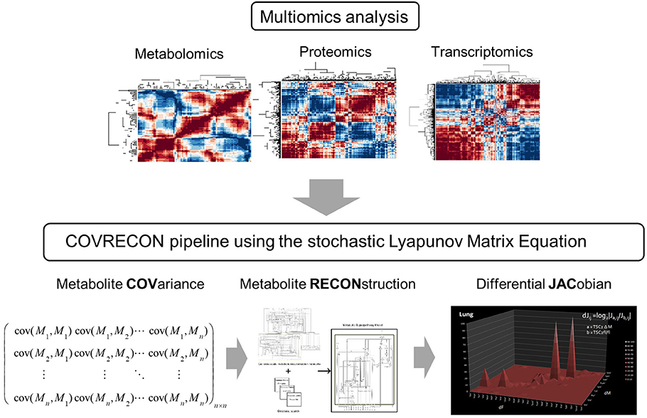
Figure 1. A workflow which combines multiomics analysis [36] and causal modeling [22] of molecular co-regulation (also called correlation or association) networks. Because the linkage of genome-scale metabolic reconstruction (RECON) and the data covariance matrix (COV) is central in this approach we call it COVRECON. The calculation of the differential Jacobian is demonstrated for the first time by Sun and Weckwerth [22].

Another very prominent example of functional annotation of genomes derives from genome-wide association studies (GWAS). Here, allelic polymorphisms in the genome of one species and its corresponding ecotypes or phenotypes are screened systematically to reveal their correlation with phenotypic and adaptive traits. In most cases, single-nucleotide polymorphisms (SNPs) are molecular neutral mutations; however, there are phenomena such as linkage disequilibrium and accumulation of SNPs in a specific genomic region pointing to potential adaptation processes in the genome [24–28]. Initially, these potentially functional SNPs are revealed by correlation analysis with phenotypic traits, and in a tedious and laborious way, these spurious correlations need to be tested for their causal relevance. A very elegant study has demonstrated the full workflow 2008 in maize starting with GWAS and finally identifying the causal relationship in some maize seeds [29]. Other studies have combined GWAS and metabolomics to identify causal genes involved in the human metabotype [30]. We have recently applied in situ eco-metabolomics in combination with SNP enrichment and metabolic modeling to reveal potential biochemical adapation processes of Arabidopsis thaliana to the natural habitate and micro-environment [31]

The final and conclusive step to link genome-scale molecular analysis with genome sequence information is model building [12]. These models can be pure structural, kinetic, or mixed forms, which allow one to analyze the stability of the system by systematically perturbing kinetic parameters [32, 33].

However, all these approaches rely on “speculated” forward conjectures about network structure and kinetic parameters. The problem is that all these data are not available, especially the detailed kinetics of protein interaction, enzymatic reactions, and biochemical regulation. We have recently introduced a novel idea by linking correlation networks of molecular components in an organism with the underlying biochemical regulation [34]. The dynamic molecular interaction or correlation networks are derived by applying the comprehensive PANOMICS platform introduced above and using statistics to reveal correlations between the components [34–38] (Figure 2). Here, the terminus correlation is equivalent to covariance, co-regulation or association often used in literature. Any kind of pairwise correlation analysis or multivariate statistical analysis is using the same basic assumption that there is a relation between the components that can be resolved by statistics. In a second step, we use genome data for a metabolic reconstruction as introduced above [12, 17]. The linkage of the molecular correlation networks and the genome-scale metabolic reconstruction somehow fills the static information of the genome with life. Eventually, we have demonstrated in 2012 that one can use the molecular covariance networks to calculate the biochemical perturbation of the system using the inverse stochastic Lyapunov matrix equation [22] (Figure 1). In several follow-up studies, we have demonstrated that the “calculated” predictions—in contrast to “speculated” predictions—reveal biochemical key points of regulation [16, 39–41]. Also, other groups have used the proposed concept to predict biochemical perturbation [42, 43]. The aim of the following paragraph is to demonstrate that the concept of the stochastic Lyapunov matrix equation is systematically derived from very basic system-theoretical principles, thereby presenting a fundamental system-theoretical equation.

FIGURE 2

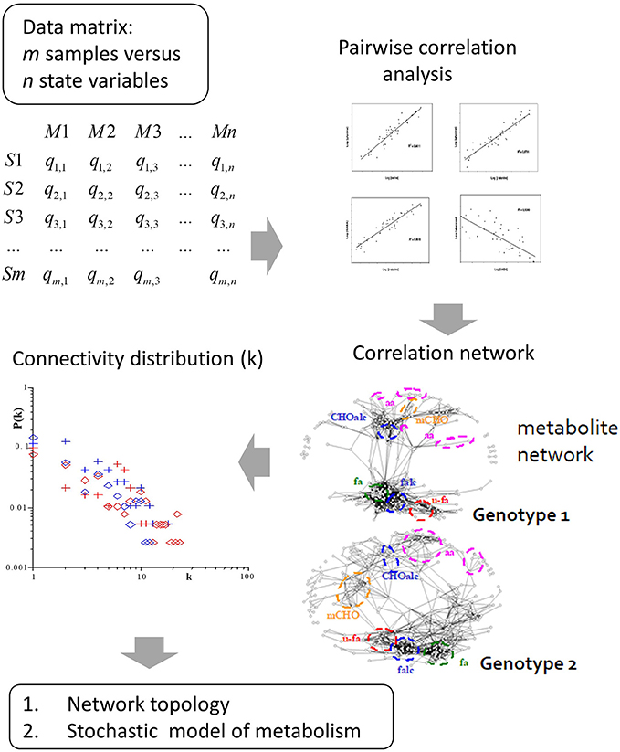
Figure 2. Derivation of metabolite correlation networks from large-scale metabolomic analysis. These correlation networks show differential connectivity in dependence of the analyzed genotype. From this fundamental multivariate structure several research fields are envisioned: Firstly, topology analysis of the correlation network resulted in a power-law-like pattern of the probability of metabolite connectivity [34, 35]. The power-law pattern is observed in real world networks with only a few hub nodes showing high connectivity in contrast to most others. This pattern is also highly conserved in biochemical networks, thus reflecting biochemical network structure and regulation. Secondly, based on the correlation pattern we developed a stochastic model of metabolism which led to the stochastic Lyapunov matrix equation (for more details see text).

A Statistical–Mathematical Formalism to Streamline Biological and Ecological Multivariate Data Causality Analysis

The pioneering work of Bertalanffy and others still provides the basic principles necessary to analyze any complex biological and ecological system. These principles were developed in parallel and multidisciplinary, e.g., in the work of Ludwig v. Bertalanffy in biology in the 1930s, or in the work of Alfred Lotka in ecology in 1934, and later by the work of Norbert Wiener in cybernetics and many others. Parts of stable population theory were already introduced by Leonard Euler in 1760 as discussed in Lotka's seminal work [44]. Principally, Bertalanffy, Lotka, and all others generalized any complex system by applying general systems equations [3, 44]. Because the basic principles of systems analysis are built on the work of Newton, Leibniz, and Euler, I will introduce briefly these formalisms. However, it has to be considered that there are important differences depending on the system under study: in Newton's world, velocity and acceleration of particles in a Euclidian space are considered. In biology, for instance, we consider molecular dynamics and phenotypes in the organismic phase space, and in ecology, we consider, e.g., population dynamics and prey/predator phase spaces. It is already clear from this that it is not yet possible to define and observe the complete system at once. Accordingly, the accurate initial definition of the “sub”-system under study and its relation to the environment is of utmost importance [45, 46]. A very intriguing discussion is found in Günter Ropohl's book, Allgemeine Systemtheorie [47].

From the mathematical point of view, the system under study is instantaneously defined by its state variables that can be measured [45]. These state variables—number of individuals in populations, metabolite concentrations, etc.—span a coordinate system that can be understood as the phase space of the system. Accordingly, the measurements of these state variables represent exclusive solutions of the respective system. Typically, we analyze and characterize these solutions by multivariate statistics such as correlation networks, principal, or independent components analysis of many biological replicates of a fluctuating quasi steady state of the system [12, 17, 18, 34, 36, 37]. Here, we and all other labs observed the phenomenon that many biological replicates of the “same” system state by snapshot analysis of the metabolome, proteome, or transcriptome showed high biological variance that can be exploited for variance and covariance analysis to distinguish the time-dependent molecular states of the system [18–20, 35, 36, 42, 48, 49] (see Figures 3–6). Importantly, these trajectories built from distinct covariance matrices of the measured n variables—genes, proteins, metabolites, phenotypes, populations, etc.—represent solutions in this n-dimensional space, which is spanned by these n state variables. As we do not know the systems equation that would enable the calculation of the interactions and dynamics of the state variables in the system, we can instead learn more about the systems equations by exploiting the “statistical solutions” of the system in an inverse approach. This can be achieved in approximation by calculation of the Jacobian at the fix points or quasi equilibrium/steady states of the system that are directly or transiently related to the “covariance solutions” of the system. As the Jacobian is defined by the systems equation, we can learn about these equations by inverse calculation of the Jacobian from the “covariance solution” using the stochastic Lyapunov matrix equation [22]. We call this data-driven inverse modeling strategy COVRECON (Figure 1). I will explain the principal concepts and workflows step by step in the following paragraphs.

FIGURE 3

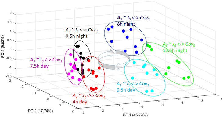
Figure 3. A PCA plot showing the metabolomic trajectory of a diurnal cycle of Arabidopsis thaliana [37]. The independent biological replicates reach again and again the same quasi-steady state (the circles) in the phase space. From these replicate analysis a covariance matrix can be obtained for each time point (Cov₁-Cov₆). From all these different covariance matrices a corresponding Jacobian (J₁-J₆) can be calculated with the inverse stochastic Lyapunov matrix equation showing the biochemical perturbation and keypoints of control over a day-night cycle (for more details see text).

Irrespective of which system we are analyzing, the basic systems equations are derived always in exactly the same way. Bertalanffy, Lotka, and all others used first-order coupled ordinary differential equations (ODEs) as the mathematical formalism. A very intuitive and elegant description is found by Uwe an der Heiden [46]. To understand the mathematical formalism, it is helpful to start with the analysis of a rather abstract linear system introduced by Newton, e.g., a coupled mass–spring system of higher order with damping coefficients, and then extrapolate the analytical solutions to numerical solutions and finally to stochastic non-linear systems by calculating the Jacobian at quasi equilibrium.

Let us start with the coupled mass–spring system. Later on, this simple system consisting of one mass, one spring, and a damping coefficient can be extended to a highly complex system: imagine a chain or network of thousands or millions of coupled mass–spring systems and various damping terms [51, 52]. This kind of network of n interacting components and properties can be described by an nth-order master equation or a corresponding dissected set of coupled first-order differential equations and is therefore comparable to any other complex system of interacting components, molecules, phenotypes, populations, or even state variables of economic systems (Figure 6).

A damped mass–spring system is described by a second-order differential equation:

\begin{array}{l} M \frac{d^{2} x}{d t^{2}} + D \frac{d x}{d t} + K x = 0 & (1) \end{array}

with $\frac{d x}{d t}$ as the velocity and $\frac{d^{2} x}{d t^{2}}$ as the acceleration and M, D, and K as system parameters.

Correspondingly, higher-order systems result in nth-order systems [52–54]:

\begin{array}{l} a_{n} \frac{d^{n} x}{d t^{n}} + a_{n - 1} \frac{d^{n - 1} x}{d t^{n - 1}} + \dots + a_{2} \frac{d^{2} x}{d t^{2}} + a_{1} \frac{d x}{d t} + a_{0} x = 0 & (2) \end{array}

One could think about networks of coupled mass–spring systems. Their interaction matrix is characterized by the incidence matrix [51, 54, 55]. A similar idea is the “community matrix” of population dynamics, firstly introduced by Richard Levins and further discussed by Robert May in ecosystems analysis (see also below) [56, 57]. Because any system we can think of is a dynamic network of its interacting components, this initial step is fundamental for deriving a quantitative understanding. By introducing new variables and their first-order derivatives, it is possible to dissect this nth-order system and any other higher-order system into n coupled first-order differential equations [51, 53–55], e.g.,

\begin{array}{l} \begin{matrix} x_{1} = x \\ x_{2} = \frac{d x}{d t} \\ x_{3} = \frac{d^{2} x}{d t^{2}} \\ ⋮ \\ \frac{d x_{1}}{d t} = x_{2} \\ \frac{d x_{2}}{d t} = x_{3} \\ ⋮ \\ \frac{d x_{n - 1}}{d t} = x_{n} \\ \frac{d x_{n}}{d t} = - a_{n - 1} x_{n} - a_{n - 2} x_{n - 1} - \dots - a_{2} x_{3} - a_{1} x_{2} - a_{0} x_{1} \end{matrix} & (3) \end{array}

In matrix notation, this is

\frac{d}{d t} [\begin{array}{l} x_{1} \\ x_{2} \\ x_{3} \\ . \\ . \\ . \\ x_{n - 1} \\ x_{n} \end{array}] = [\begin{matrix} 0 & 1 & 0 & 0 & \dots & 0 & 0 \\ 0 & 0 & 1 & 0 & \dots & 0 & 0 \\ 0 & 0 & 0 & 1 & \dots & 0 & 0 \\ ⋮ & ⋮ & ⋮ & ⋮ & ⋱ & ⋮ & ⋮ \\ 0 & 0 & 0 & 0 & \dots & 0 & 1 \\ - a_{0} & - a_{1} & - a_{2} & - a_{3} & \dots & - a_{n - 2} & - a_{n - 1} \end{matrix}] [\begin{array}{l} x_{1} \\ x_{2} \\ x_{3} \\ . \\ . \\ . \\ x_{n - 1} \\ x_{n} \end{array}] (4)

\begin{array}{l} \frac{d X}{d t} = A X, & (5) \end{array}

respectively [54, 55]. A is the system matrix.

These systems are solved by inserting

\begin{array}{l} \begin{matrix} x (t) = e^{λ t} \\ \frac{d x}{d t} = λ e^{λ t} \\ \frac{d^{2} x}{d t^{2}} = λ^{2} e^{λ t} \\ ⋮ \end{matrix} & (6) \end{array}

and deriving the characteristic equation for the calculation of the eigenvalues λ_{1, 2, …, n} and constants C_{1, 2, …., n} using n initial conditions [54, 55], finally leading to the general solution:

\begin{array}{l} x (t) = C_{1} e^{λ_{1} t} + C 2 e^{λ_{2} t} + \dots + C_{n} e^{λ n t} & (7) \end{array}

The eigenvalues of the matrix A in (5) are the roots of the characteristic equation [52]. One can substitute the zeros in the matrix A if there are off-diagonal connections between the state variables (see discussion below). These matrix systems of linear differential equations [Equation (5)] can be solved by the eigenvector/eigenvalue equation. Suppose the n by n matrix A has n linearly independent eigenvectors. Then,

\begin{array}{l} T^{- 1} A T = D & (8) \end{array}

with the eigenvector matrix T and the eigenvalue matrix D [52, 54].

The solution of Equation (5) is according to Equations (7, 8) in matrix notation:

\begin{array}{l} X (t) = T e^{D t} T^{- 1} X (0) & (9) \end{array}

and corresponds to the matlab command [T,D] = eig(A) [52].

Linear systems (5) can be solved by (8) and (9) calculating the eigenvalues and eigenvectors. In case of nonlinear systems equations which is true for almost all molecular, organismal and ecological networks in the real world we have to introduce the Jacobian matrix. The Jacobian matrix is derived by linearizing a non-linear system at quasi steady states [52, 54]. Assume a non-linear function

\begin{array}{l} \frac{d x}{d t} = f (x) & (10) \end{array}

with the steady state

\begin{array}{l} f (x_{0}) = 0 & (11) \end{array}

For x near x₀,

\begin{array}{l} s o Δ x = x - x_{0} \end{array}

is small, a Taylor expansion leads to

\begin{array}{l} f (x) ~ {\frac{D f}{D x} |}_{x = x_{0}} (x - x_{0}) & (12) \end{array}

Which is called the “Jacobian” [54, 58]. For an n-dimensional system the Jacobian matrix reads:

\begin{array}{l} J (x_{0}) = [\begin{matrix} \frac{\partial f_{1}}{\partial x_{1}} & \frac{\partial f_{1}}{\partial x_{2}} & \dots & \frac{\partial f_{1}}{\partial x_{n}} \\ \frac{\partial f_{2}}{\partial x_{1}} & \frac{\partial f_{2}}{\partial x_{2}} & \dots & \frac{\partial f_{2}}{\partial x_{n}} \\ ⋮ & ⋮ & \dots & ⋮ \\ \frac{\partial f_{n}}{\partial x_{1}} & \frac{\partial f_{n}}{\partial x_{2}} & \dots & \frac{\partial f_{n}}{\partial x_{n}} \end{matrix}] & (13) \end{array}

For linear systems or close to the steady state, it holds

\begin{array}{l} J ~ A & (14) \end{array}

The solution to these systems is again given by the matrix eigenvalue/eigenvector Equation (10) [52, 54, 55]:

\begin{array}{l} T^{- 1} A T = D & (8) \end{array}

Once we derive the Jacobian of a system of coupled first-order differential equations, we can calculate eigenvalues and vectors, which describe stability and system properties close to a steady state or quasi equilibrium. If we are able to derive the Jacobian from the covariance matrix of the data (see below), we can calculate the eigenvalues from these data-derived Jacobians to investigate their properties. For this we have developed the concept of the inverse stochastic Lyapunov matrix equation and we have recently tested this idea [16, 22, 59]. In the following this concept is explained. To solve this inverse problem we need to exploit the statistical solution of the system defined by the data matrix of the state variables at a steady state (or better quasi-steady state), e.g., in form of the data covariance matrix, and need to translate this into the “systems state equations solutions” represented by the Jacobian. The system dynamics at different steady states or snapshots are comprised in a nxm data matrix of n state variables at m time points or m specific sample states.

\begin{array}{l} X_{D} = {[\begin{matrix} ⋮ & ⋮ & ⋮ & ⋮ \\ x_{1} & x_{2} & \dots & x_{m} \\ ⋮ & ⋮ & ⋮ & ⋮ \end{matrix}]}_{n x m} & (15) \end{array}

The variance–covariance matrix of the data Cov is expressed as the inner product of the centered data matrix X_Dcent:

\begin{array}{l} C o v = \frac{1}{m} X_{D c e n t} X_{D c e n t}^{T} & (16) \end{array}

If we statistically analyze several measurements or empirical observations of the state variables over time, e.g., in a principal components analysis (PCA), then we derive the trajectory of different snapshots of transitory steady states of the system defined by the covariance matrix of its state variables [12, 17, 18, 34, 37, 39, 60] (Figure 3). These trajectories are representative for the phase space of the system. In a time–dependent trajectory of a biological system or any other system, independent replicated measurements of the state variables reach a quasi-steady state represented by the corresponding state variables variance–covariance matrix at this specific time point (Figure 3). The variance of the replicated measurements around a mean value is due to unknown stochastic processes and can be approximated by stochastic simulation, e.g., adding white noise. The potential causal relation of the state variables is reflected in the covariance pattern.

To learn about the system from these data-defined trajectories [61], we need an equation that links the covariance matrix of the state variables with the Jacobian. This relationship is characterized by a special form of the Lyapunov matrix equation introducing white noise in the system and solving for the symmetric m × m covariance matrix Cov [50, 62–64] (Figure 4).

FIGURE 4

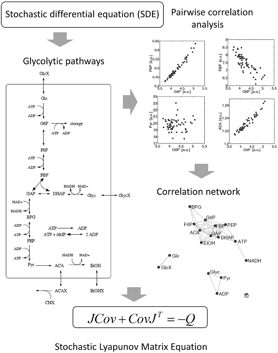
Figure 4. Derivation of the stochastic Lyapunov Matrix Equation from fluctuating metabolic correlation networks [50]. Stochastic processes are introduced by adding Gaussian white noise to the ODE. Numerical solutions of independent replicates of the system demonstrate significant pairwise correlations between metabolites according to the experimental observations in real metabolomics data (see Figure 2). The concept is described by the stochastic Lyapunov matrix equation (for more details see text).

Again, we start with Equation (5)

\begin{array}{l} \frac{d X}{d t} = A X & (5) \end{array}

The equilibrium of this system is stable in the sense of Lyapunov if there exists a continuously differentiable scalar function V(x) along the system trajectories with [64, 65]

\begin{array}{l} \begin{matrix} V (x) > 0 \\ V (0) = 0 \end{matrix} & (17) \end{array}

and

\begin{array}{l} \frac{d V}{d t} = \frac{\partial V}{\partial x} \frac{d x}{d t} \leq 0 & (18) \end{array}

If condition (18) is a strict inequality, then the equilibrium point is asymptotically stable.

For the linear system (5), a quadratic Lyapunov function can be chosen

\begin{array}{l} \begin{matrix} V (x) = x^{T} P x \\ P = P^{T} > 0 \end{matrix} & (19) \end{array}

Inserting Equation (5) leads to

\begin{array}{l} \frac{d V}{d t} = x^{T} (A^{T} P + P A) x & (20) \end{array}

This system is asymptotically stable if

\begin{array}{l} A^{T} P + P A < 0 & (21) \end{array}

\begin{array}{l} \begin{matrix} A^{T} P + P A = - Q \\ Q = Q^{T} \end{matrix} & (22) \end{array}

where Q is any positive definite matrix. For stochastic linear systems driven by white noise, the solution of the Lyapunov equation represents the variance of the state vector [64, 66]. Because of Equation (14) A~J at equilibrium or close to steady state (see above), we can now substitute A with J and P with the variance–covariance matrix Cov [64], resulting in the equation

\begin{array}{l} J C o v + C o v J^{T} = - Q & (23) \end{array}

Typically, this equation is used in the forward approach for deriving an unknown covariance matrix Cov by knowing the systems equations resulting in the Jacobian J—as described above—and the diffusion matrix Q representing the fluctuation or perturbations of the system around a steady state or critical point [62, 67]. Furthermore, this equation is also central in the theory of stochastic processes [66, 68] and has been solved by various approaches [69–71]. We derived and applied this equation to the best of our knowledge for the first time in the context of molecular correlation networks [50] (Figure 4) and developed an approach to use this equation inversely and calculate the Jacobian J from the covariance matrix Cov [22] (Figure 1). Based on a functional interpretation of this equation in the molecular context, it also represents a genotype–environment–phenotype relationship similar to the community–stability relationship in ecosystems as first described by Levins and May [56, 57, 72]. In the following paragraphs, I will explain these relationships.

A Data-Driven Inverse Modeling Approach to Solve for J Using the Stochastic Lyapunov Matrix Equation

As discussed above, Equation (23) is typically used in the forward approach for deriving an unknown covariance matrix Cov by knowing the systems equations in form of the Jacobian J. Using Equation (23) in an inverse approach, in other words, calculating the Jacobian J from a given covariance matrix Cov and diffusion matrix Q, introducing stochastic fluctuation is rather unexplored, especially in the context of molecular networks. We recently applied the stochastic Lyapunov matrix equation to the analysis of metabolic networks [22, 50] and addressed this question. We were interested in solving this equation in the reverse or inverse direction, calculating the Jacobian from the covariance matrix. This is an underdetermined problem and therefore impossible by first inspection because J has many more entries than the covariance matrix and only parameterized solutions are possible [50]. In 2012, we developed an approach based on the assumption that a typical network—metabolic network or other molecular networks—is sparse [22]. This time, we were able to calculate the Jacobian from the covariance matrix because the system of linear homogenous equations changed from an underdetermined to an overdetermined problem [22]. This was the first time that we could solve for the Jacobian J and thereby estimated differences in the matrix of systems equations starting with a covariance matrix of state variables Cov. We applied this strategy to several molecular systems [12, 16, 17, 22, 34, 39–41, 50, 59, 73]. Because the molecular interaction matrix underlying the Jacobian strictly depends on whole-genome metabolic reconstruction [12], this equation also presents a genotype–phenotype equation (Figures 1, 5).

FIGURE 5

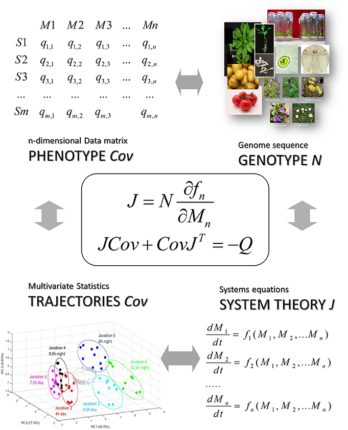
Figure 5. The stochastic Lyapunov matrix equation presents a genotype-phenotype equation. Here N is the metabolic interaction matrix or stoichiometric matrix which is derived from a whole-genome metabolic reconstruction (see also Figure 1 and [12]), Cov is defined by the data matrix and the systems equation are represented by the Jacobian which is the linearized solution of this non-linear system at a quasi-equilibrium point and reflected by the time-dependent trajectory of the system (see Figure 3) (for more details see text).

The Stochastic Lyapunov Equation Represents a Genotype–Environment–Phenotype Equation in the Framework of Model Predictive Control

Sample classification and rapid diagnostics of newborns based on metabolic profiling using gas chromatography coupled to mass spectrometry (GC–MS) is a very old technology dating back to the 1970s [74]. However, the basic idea of using metabolomic analysis to study gene function analysis emerged rather in the times when genome sequences started to be available at the beginning of the twenty first century [34, 49, 75, 76]. Accordingly, in pioneering studies, metabolomics was applied in combination with multivariate statistical analysis to study gene mutants especially in plants and yeast [35, 48, 77]. An intriguing approach for the analysis of these multivariate data matrices has been the construction of correlation networks [34, 35, 38, 49, 78]. From 2000 on we systematically investigated the structure and biochemical relevance of metabolite correlation networks and revealed generic topological properties such as a power-law-like distribution of metabolite connectivity (see Figure 2) [35]. By realizing that biological replicate analysis showed an intrinsic high variance of the corresponding state variables, we developed a modeling approach that implements stochastic differential equations (SDEs) for the simulation of metabolic networks [50]. The use of SDEs mimics the situation of intrinsic fluctuation of metabolite levels within the analyzed system as discussed above. Because we did not know the very specific origin of this fluctuation, we have used Gaussian white noise with zero mean and unit variance (Figure 4). The partial differential equation for the time evolution of the probability density function of this stochastic system is described by the Fokker–Planck or Kolmogorov or Diffusion equation [50, 66]. Also, Robert May derived this relationship for the description of population dynamics in randomly fluctuating environments [57]. I will discuss this in the last paragraph in more detail. Setting this equation to zero results in the approximate equilibrium probability distribution of the fluctuating state variables, in our case, metabolite concentrations. The resulting m × m covariance matrix Cov of the state variables can be seen to be the solution of the stochastic Lyapunov matrix equation (21) (Figure 4) [50]. The starting point of this computer simulation has been the observation of strong biological fluctuations in metabolite concentrations. Based on this stochastic model, we could explain the existence of these metabolite correlation networks and also their relation to the underlying biochemical network. However, a major aim was to calculate the underlying regulation—in other words, the Jacobian—from the metabolite covariance data. This was not possible, but instead, we showed a parameterized solution to the problem. We finally solved this problem by assuming that metabolic networks are highly sparse networks that allowed the calculation of the Jacobian directly from the metabolomics data (Sun and Weckwerth [22]). Because the Jacobian structure of biochemical networks is defined by the stoichiometric or metabolic interaction matrix of the genotype-based reconstructed metabolic network, it contains all the information of potential causal relations of this specific genotype (Figure 5) (for more details of this relationship, see Weckwerth [12, 17, 74]). In Figure 1 the COVRECON strategy shows the systematic linkage of genome-scale metabolic reconstruction, multiomics measurement of state variables of the system and the inverse Lyapunov matrix equation for functional data integration. Because this equation explicitly describes the relation of the Jacobian and the data covariance matrix, it connects all other multivariate properties of the system such as pairwise state variable correlations, metabolite correlation networks, and time-dependent trajectories of the system derived from PCA (Figure 6 and discussion below). This basically holds true for any complex system from biology, ecology, economy, and sociology (see Figure 6) and even for model predictive control of artificial intelligence systems (see below). Therefore, the stochastic Lyapunov matrix equation and especially its inverse application are based on intrinsic systemic properties and represent a fundamental equation in system theory.

FIGURE 6

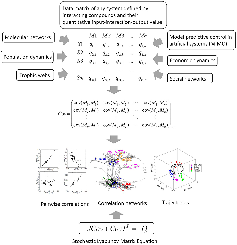
Figure 6. The data matrix and the stochastic Lyapunov matrix equation are directly associated by multivariate properties of the system. This applies to any complex network or system and even to model predictive control of artificial intelligence systems. MIMO, multiple input multiple output.

Importantly, the approach is especially suited for non-linear systems, multiple stability, and limit cycle analysis because it uses the data covariance matrix—thus the real data of a biological system where we assume it is in quasi steady state—to predict the system matrix. Thus, any calculated quasi steady state is a realistic solution of the system because it relies on the real data at least in biological systems. This is very much related to model predictive control of non-linear and closed loop artificial systems using the stochastic Lyapunov matrix equation [79, 80], which demonstrates that the proposed framework is appropriate for closed loop and limit cycling control analysis. Moreover, Lyapunov-based control analysis is nowadays becoming more and more attractive for bioinspired artificial intelligence systems [81, 82]. This also gives rise to another hypothesis whether control parameters of biological systems with or without limit cycles can be revealed by this inverse approach. All conventional approaches start with an existing model. We use the empirical data to reveal the model control points by calculating the system matrix J from the data covariance matrix and looking for specific perturbations in J from one state to a consecutive or perturbed next state of the system [16, 22, 39, 40]. In the future, we will analyze hypothetical closed loop systems such as the diurnal rhythm of a plant or circadian regulation of cellular metabolism to test for this hypothesis.

PCA Is Bound to the Jacobian System Matrix of a Non-Linear System by the Inverse Stochastic Lyapunov Matrix Equation—Modeling Meets Big Data Science

The stochastic Lyapunov matrix equation also provides the basis for the functional interpretation of PCA of molecular data. As the covariance matrix Cov of the measured state variables is the underlying information of PCA, it can be assumed that there is a direct link of Equation (23) and PCA or, in other words, the analysis of the systems trajectory in the phase space (see section before). Indeed, Cov is derived from the data matrix X_D by Equation (16). Cov can be dissected by singular value decomposition (SVD) formalism or eigendecomposition [51, 54, 55]:

\begin{array}{l} C o v = U Σ U^{T} & (24) \end{array}

Here, U—the eigenvectors of the symmetric covariance matrix—corresponds to the “loadings” of a PCA and Σ —the squared eigenvalues of Cov_D—corresponds to the “scores” [51, 52].

Now, we can insert Equation (24) into Equation (23) and obtain a direct relation of PCA and the Jacobian of the data

\begin{array}{l} J U Σ U^{T} + U Σ U^{T} J^{T} = - Q & (25) \end{array}

This equation establishes the direct linkage of PCA and the biochemical Jacobian (Figure 3). More important, this principle holds true for any other complex system as well—from molecular, ecological, up to economic or sociological networks (see Figure 6).

SVD, PCA, and many related tools are basic algorithms for the analysis of large-scale data with millions of data points and/or millions of variables. Therefore, these conceptual Equations allow for the data-driven calculation of solutions of the underlying general system of first-order differential equations once we have assumptions about the underlying interaction networks. Consequently, we can test any complex system for data-driven generic principles.

We have implemented this approach and demonstrated the feasibility to identify causal relationships in highly complex molecular association networks [16, 22, 39, 41, 73, 73, 83].

Furthermore, the calculation of the Jacobian from the data matrix and the covariance matrix, respectively, allows for the data-driven analysis of stability and control of trajectories of these systems [59]. Knowing the trajectory of the system's state variables from the measured or observed data, one is able to learn about the underlying principles and system equations.

Many obstacles remain. The calculation of the Jacobian is highly dependent on the accuracy of the covariance matrix. A perfect covariance matrix will reveal the perfect solution of the Jacobian; however, the data are in most instances too noisy to guarantee the best solution. Therefore, many data points are necessary to establish a reasonable covariance matrix. Furthermore, the calculation is highly dependent on the condition number of the system. Ill-conditioned systems are problematic [73]. Therefore, a reduction to superpathways or highly generic and reduced interaction or better incidence matrices, e.g., is a solution to the problem [16, 39].

The Stochastic Lyapunov Matrix Equation Is a Fundamental Principle for the Complexity–Stability Relationship of Ecological Systems Using SDEs and Random Matrix Theory

The proposed concept of systematic inverse calculation of the Jacobian from data covariance has not been applied in ecological or population studies to the best of my knowledge. Thus, one further hypothesis is that this concept could be exploited as a general framework from molecular biology to ecological systems analysis. This idea is especially supported by the following studies. In 1970, Gardner and Ashby presented an intriguing analysis of the connectance—nowadays called connectivity (see Figure 2)—of large dynamic systems and investigated their stability [84]. Inspired by this work as one of the first systematic analyses of network connectivity, Robert May presented a follow-up study and translated this idea into the ecological context for the analysis of complex population dynamics using random matrix theory [72]. May described a system with n variables, which are the n populations of interacting species. This system and its stability close to equilibrium are characterized by the equation

\begin{array}{l} \frac{d X}{d t} = A X & (5) \end{array}

with X as the nx1 column vector of the disturbed populations x_j and the nxn interaction matrix A with elements a_jk describing the effect of species k on species j near equilibrium. The interaction network of populations defines whether there is an interaction or not (a_jk = 0) and the type of interaction defines the sign and magnitude of a_jk. The population average interaction strength mean square value α and the connectance (connectivity) C are drawn randomly from a statistical distribution, and relations for the local asymptotic stability of A—all eigenvalues have negative real parts or not—are derived depending on the mean interaction strength, number of populations, and connectance (for further details, see May [72])

\begin{array}{l} α > {(n C)}^{- 1 / 2} & (26) \end{array}

The interpretation of May is famous:

“Applied in an ecological context, this ensemble of very general mathematical models of multi-species communities, in which the population of each species would by itself be stable, displays the property that too rich a web connectance (too large a C) or too large an average interaction strength (too large an α) leads to instability. The larger the number of species, the more pronounced the effect” [72].

It is intriguing that this system definition and all subsequent derivations are exactly derived from the same system-theoretical principles described above. In later discussions, Robert May implemented the stochastic Lyapunov matrix equation for the analysis of multispecies models in stochastic environments [57] by interpreting the symmetric covariance matrix Cov as the solution of the Lyapunov matrix equation. This is exactly the same interpretation as we have developed for the characterization of molecular networks [see above Equation (23)].

These general principles in studies of ecological systems and population dynamics have been extended intensively investigating the Jacobian of these systems as a central figure [85]. On the other hand, no follow-up study has tried to apply an inverse approach by deriving the Jacobian from the data covariance matrix in ecological systems. Accordingly, this will be an interesting research question for future studies.

Conclusion

The main aim of the presented ideas is to demonstrate the common system-theoretical principles of biological and ecological systems. It is intriguing how principles of the analysis of dynamical systems are originated by principles of system theory and later cybernetics and can be applied to the analysis of biological and ecological systems. A main framework is defined by stability analysis and application of the stochastic Lyapunov matrix equation. The inverse application of stochastic Lyapunov matrix equation allows for the data-driven inverse modeling of complex systems from molecular to population networks and will be further explored for the prediction of regulatory structures in these highly complex and intuitively inaccessible systems.

Author Contributions

The author confirms being the sole contributor of this work and has approved it for publication.

Conflict of Interest Statement

The author declares that the research was conducted in the absence of any commercial or financial relationships that could be construed as a potential conflict of interest.

Acknowledgments

I would like to thank Xiaoliang Sun and Thomas Nägele for all these inspiring discussions that we shared in the last years and Gerhard Sorger for helpful comments on the manuscript.

References

1. Bertalanffy LV. Vom Molekül zur Organismenwelt. Potsdam: Akademische Verlagsgesellschaft Athenaion (1944).

2. Bertalanffy LV. Der Organismus als physikalisches system betrachtet. Naturwissenschaften. (1940) 33:522–31. doi: 10.1007/BF01497764

CrossRef Full Text | Google Scholar

3. Bertalanffy LV. General System Theory. New York, NY: George Braziller. (1969).

HYPOTHESIS AND THEORY article

Toward a Unification of System-Theoretical Principles in Biology and Ecology—The Stochastic Lyapunov Matrix Equation and Its Inverse Application

Reflections on Historical Developments

Genome-scale Molecular Analysis—A PANOMICS Platform Combined With Data-Driven Modeling

A Statistical–Mathematical Formalism to Streamline Biological and Ecological Multivariate Data Causality Analysis

A Data-Driven Inverse Modeling Approach to Solve for J Using the Stochastic Lyapunov Matrix Equation

The Stochastic Lyapunov Equation Represents a Genotype–Environment–Phenotype Equation in the Framework of Model Predictive Control

PCA Is Bound to the Jacobian System Matrix of a Non-Linear System by the Inverse Stochastic Lyapunov Matrix Equation—Modeling Meets Big Data Science

The Stochastic Lyapunov Matrix Equation Is a Fundamental Principle for the Complexity–Stability Relationship of Ecological Systems Using SDEs and Random Matrix Theory

Conclusion

Author Contributions

Conflict of Interest Statement

Acknowledgments

References

People also looked at