Constrained Covariance Matrices With a Biologically Realistic Structure: Comparison of Methods for Generating High-Dimensional Gaussian Graphical Models
 Frank Emmert-Streib
 Shailesh Tripathi
 Matthias Dehmer
- 1Predictive Society and Data Analytics Lab, Faculty of Information Technology and Communication Sciences, Tampere University, Tampere, Finland
- 2Institute of Biosciences and Medical Technology, Tampere, Finland
- 3Faculty for Management, Institute for Intelligent Production, University of Applied Sciences Upper Austria, Steyr, Wels, Austria
- 4Department of Mechatronics and Biomedical Computer Science, UMIT, Hall in Tyrol, Austria
- 5College of Computer and Control Engineering, Nankai University, Tianjin, China
High-dimensional data from molecular biology possess an intricate correlation structure that is imposed by the molecular interactions between genes and their products forming various different types of gene networks. This fact is particularly well-known for gene expression data, because there is a sufficient number of large-scale data sets available that are amenable for a sensible statistical analysis confirming this assertion. The purpose of this paper is two fold. First, we investigate three methods for generating constrained covariance matrices with a biologically realistic structure. Such covariance matrices are playing a pivotal role in designing novel statistical methods for high-dimensional biological data, because they allow to define Gaussian graphical models (GGM) for the simulation of realistic data; including their correlation structure. We study local and global characteristics of these covariance matrices, and derived concentration/partial correlation matrices. Second, we connect these results, obtained from a probabilistic perspective, to statistical results of studies aiming to estimate gene regulatory networks from biological data. This connection allows to shed light on the well-known heterogeneity of statistical estimation methods for inferring gene regulatory networks and provides an explanation for the difficulties inferring molecular interactions between highly connected genes.
1. Introduction
High-throughput technologies changed the face of biology and medicine within the last two decades [1–3]. Whereas traditional molecular biology focused on individual genes, mRNAs and proteins [4], nowadays, genome-wide measurements of these entities are standard. As an immediate consequence, transcriptomics, proteomics, and metabolomics data are high-dimensional containing measurements of hundreds and even thousands of molecular variables [5–10]. Aside from the high-dimensional character of these data, there exists a non-trivial correlation structure among the covariates, which establishes considerable problems for the analysis of such data sets [11–13]. The reason for the presence of the correlation structure is due to the underlying interactions between genes and their products. Specifically, it is well-known that there are transcriptional regulatory, protein, and signaling networks that represent the blueprint of biological and cellular processes [14–20].
In order to design new statistical methods, which are urgently needed to cope with high-dimensional data from molecular biology, usually, simplifying assumptions are made regarding the characteristics of the data. For instance, one of the most frequently made assumptions is the normal behavior of the covariates [21–24]. That means, the distribution of the variables is assumed to follow a univariate or multivariate normal distribution [25]. This assumption is reasonable because by applying a z-transformation to data with an arbitrary distribution one can obtain (standard) normal distributed data [26]. For this reason, a z-transformation is usually applied to the raw data as a preprocessing step. Due to the fact that we investigate in this paper high-dimensional data with a complex correlation structure, we focus in the following on multivariate normal distributions, because to use a univariate distribution in this context, it is necessary to make the additional assumption of a vanishing correlation structure between the covariates in order to be able to approximate the multivariate distribution sensibly by a product of univariate distributions, i.e., .
To fully specify a multivariate normal distribution, a vector of mean values and a covariance matrix is needed. From the covariance matrix follows the correlation matrix that provides information about the correlation structure of the variables. For instance, for data from molecular biology measuring the expression of genes, it is known that the correlation in such data sets is neither vanishing nor random, but is imposed by biochemical interactions and bindings between proteins and RNAs forming complex regulatory networks [27, 28]. For this reason, it is not sufficient to merely specify an arbitrary covariance matrix in order to simulate gene expression data from a norm distribution for investigating statistical methods, because such a covariance matrix is very likely not to possess a biologically realistic correlation structure. In fact, it is known that biological regulatory networks have a scale-free and small-world structure [29, 30]. For this reason, several algorithms have been introduced that allow to generate constrained covariance matrices that represent specific independence conditions, as represented by a graph structure of gene networks. If, for instance, a gene regulatory network or a protein interaction network is chosen for such a network structure, these algorithms generate covariance matrices that allow to generate simulated data with a correlation structure that is consistent with the structural dependency of such biological networks, and hence, is close to real biological data [31, 32]. Here “consistent” means that for multivariate normal random variables there is a well-known relation between the components of the inverse of their covariance matrix and their partial correlation coefficients, discussed formally in the section 2. This relation establishes a precise connection between a correlation structure in the data and a network structure. As a result, such a constrained covariance matrix establishes a Gaussian graphical model (GGM) [33, 34] that can be used to simulate data for the analysis of, e.g., methods to identify differentially expressed genes, differentially expressed pathways or for the inference of gene regulatory networks [11, 35–37], to name just a few potential areas of application.
The major purpose of this paper is to study and compare three algorithms that have been introduced to generate constrained covariance matrices. The algorithms we are studying are the Iterative Proportional Fitting (IPF) algorithm [38], an orthogonal projection method by Kim et al. [37] and an regression approach by Hastie, Tibshirani, and Friedman (HTF) [39]. Data generated by such algorithms can be used to simulate, e.g., gene expression data from DNA microarrays to test analysis methods for identifying differentially expressed genes [22, 40], differentially expressed pathways [41–43] or to infer gene regulatory networks [44, 45]. Furthermore, we connect these results, obtained from a probabilistic perspective, to statistical results of studies aiming to infer gene regulatory networks. This connection allows to shed light on the known heterogeneity of statistical estimation methods for inferring gene regulatory networks.
The paper is organized as follows. In the next section, we present the methods we are studying and necessary background information. This includes a description of the three algorithms IPF, Kim, and HTF to generate constrained covariance matrices and also a brief description of the networks we are using for our analysis. In the sections 3 and 4, we present our numerical results and discuss the observed findings. Furthermore, we place the obtained results into a wider context by discussing the relation to network inference methods. This paper finishes in the section 5 with a summary and an outlook to future studies.
2. Methods
Multivariate random variables, X ∈ ℝp, from a p-dimensional normal distribution, i.e., X ~ N(μ, Σ), with mean vector μ ∈ Rp and a positive-semidefinite p × p reel covariance matrix Σ, have a density function given by
For such normal random variables there is a simple relation between the components of the inverse covariance matrix, Ω = Σ−1, (also called “precision” or “concentration matrix”) and conditional partial correlation coefficients [46] (chapter 5). This relation is given by
Here ρij|N\{ij} is the partial correlation coefficient between gene i and j conditioned on all remaining genes, i.e., N\{ij}, whereas N = {1, …, p} is the set of all genes. Furthermore, ωij are the components of the concentration matrix Ω. That means, if ρij|N\{ij} = 0 then gene i and j are independent from each other,
if and only if ωij = 0. The relation in Equation (3) is also known as Markov property [46] (chapter 3). In the following, we abbreviate the notation for such partial correlation coefficients briefly as,
and denote the entire partial correlation matrix by Ψ.
A multivariate normal distribution that is Markov with respect to an undirected network G is called a Gaussian graphical model (GGM) [33, 34, 46], also known as “graphical Gaussian model,” “covariance selection model,” or “concentration graph model.” This means that all conditional independence relations that can be found in Σ−1 are also present in G [46] (chapter 3). Hence, such a Σ−1 can be considered as consistent [or faithful [47]] with all conditional independence relations in G.
2.1. Generation of a Random Covariance Matrix Using Conditional Independence for a Given Graphical Model
In the following, we describe briefly the three algorithms IPF, Kim and HTF [37, 38, 46, 48], we use for generating constrained covariance matrices that are consistent with a given graph structure by obeying its independence relations.
Kim Algorithm: The Kim algorithm [37] applies iteratively orthogonal projections to generate a covariance matrix with the desired properties. A formal description of this algorithm is as follows:
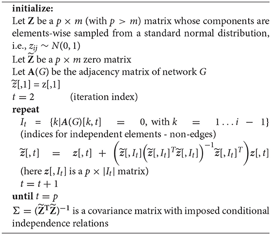
Algorithm 1 Generation of a constrained covariance matrix using the Kim algorithm
We are providing an R package with the name mvgraphnorm that contains an implementation of the Kim algorithm. The package is available from the CRAN repository.
Before we continue, we would like to emphasize that in the following, we use the notation W and V to indicate covariance matrices. However, the important difference is that W is unconstrained whereas V is consistent with conditional independence relations given in a network G.
IPF Algorithm: The working principles of the Iterative Proportional Fitting algorithm [38] is as follows. Let us assume that X is a p-dimensional random variables from a normal distribution with mean μ = 0 and a covariance matrix Σ. From a sample of size m, the sample covariance matrix is estimated from a given W. Suppose, we partition the vector X into Xa, Xb, for randomly selected index vectors a and b. Then these vectors, Xa and Xb, follow a normal distribution with mean μ = 0 and variance
Furthermore, the marginal distribution of Xa is normal with variance Vaa and the conditional distribution of Xb|a is also normally distributed with [46]. Let us assume that f is a given density function and g is the density function of a Gaussian graphical model with a similar marginal distribution as f.
The iterative proportional fitting (IPF) algorithm [38] adjusts iteratively the joint density function of Xa and Xb. This can be written in general form as,
corresponding to the (t + 1)th iteration step. In this notation, the expectation value of X, for , is given by,
which remains zero for all iteration steps t. For this reason, we do not need to consider update equations for this expectation value. In contrast, the variance of X, for , is given by
with [46].
The IPF algorithm, formalized in Algorithm 2, provides iterative updates for the components of the covariance matrix Vt+1, given by Equation (8). In this algorithm, the first step is to generate a sample covariance matrix W and V is initialized as identity matrix with the same number of rows and columns as W. In the second step, the maximal cliques of a given graph G are identified. Here a clique is defined as a fully connected subgraph of G. Next, the components of the partitioned covariance matrix are iteratively updated, in order to become consistent with the independence relations in G. This is accomplished by utilizing the identified cliques. This procedure is iterated for all cliques, until the algorithm converges, as specified by a scalar threshold parameter δ, with δ ≪ 1.
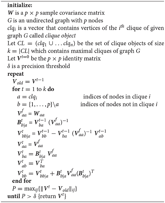
Algorithm 2 Generation of a constrained covariance matrix using the IPF algorithm
HTF Algorithms: We call the following algorithm HTF because it has been proposed by Hastie, Tibshirani, and Friedman [39]. In Algorithm 3 we show pseudocode for this algorithm.
Let us assume, we have a p-dimensional random variable, X ∈ ℝp, sampled from a normal distribution with mean μ and covariance matrix Σ, and a sample covariance matrix S estimated from m samples. The log likelihood for the (unconstrained) concentration matrix Ω is given by,
which is maximized for Ω = Σ−1.
The HTF method uses a regression approach for each node by selecting its neighbors as predictor variables, utilizing model based estimates of predictor variables. For this approach, Lagrange constants are included in Equation (9) for the non-edge components of a given graph structure,
Here j, k ∉ E means that there is no edge between these two variables, i.e., Aij = 0. We maximize this likelihood by taking the first derivative with respect to Ω, which gives
Here Γ is the matrix of Lagrange parameters with non-zero values for the non-edge components of a given graph structure.
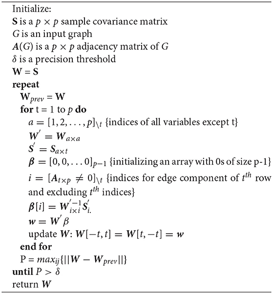
Algorithm 3 Maximum likelihood estimation of independence of a sample covariance matrix for a given graph using HTF algorithm.
Because one would like to obtain W = Ω−1, we can write this identify separated into two major components,
Here the first component consists of p − 1 dimensions and the second component of just one. That means, e.g., W12 and I are (p − 1) × (p − 1) matrices, w12 and ω12 are (p-1)-dimensional vectors and w22 and ω22 are scalar values.
The iterative algorithm of HTF repeats the steps given in Equations (11–18). At each step, one selects one of the p variables randomly for the partitioning given in Equation (12). This variable defines w12 and ω12, whereas the remaining variables define W11 and Ω11. For reasons of simplicity, we select in the following the last variable.
From Equation (12), we obtain the following expression
Setting β = ω12/ω22 and placing w12 into the right block of Equation (11), namely,
leads to
This system is solved only for the q components in β that are not equal to zero, i.e., q = |{i|βi ≠ 0}, which can be written as
Here it is important to note that and is a q×q matrix. From this, is given by
and the overall solution follows from padding with zeros in the q components given by Ip = {i|βi = 0} is β′. Finally, this is used to update w12 in Equation (13) leading to
The above steps are iterated, for each variable, until the estimates for w12 converge.
The qpgraph package by [48] provides an implementation of the IPF and HTF algorithm.
Common Step of IPF and HTF: The IPF and HTF algorithm have in common that they are based on the random initialization of a covariance matrix W that is obtained from a (parametric) Wishart distribution [49]. More precisely, assume X1, X2, …Xm are m samples from a p-dimensional normal distribution N(0, Σ), then
is from a Wishart distribution. Here n is the degrees of freedom and Σ is a p × p matrix. The expectation value of W is given by,
In order to obtain a covariance matrix W from a Wishart distribution given by , the Bartlett decomposition can be utilized given by [49–51],
Here L(r)L(r)T is obtained from a Cholesky decomposition of and A is defined by,
Here the nij ~ N(0, σ), for i ∈ {2, …, p} with i > j, and , Chi-squared distribution with p + 1 − i degrees of freedom, with i = 1…p. For reasons of simplicity, Σ(r) can be defined as
which results in a constant correlation coefficient r, with 0 ≤ r ≤ 1, between all variables. For this reason, we write the covariance matrix, and the resulting L(r) and W(r) matrices, explicitly as a function of the parameter r.
The IPF and the HTF algorithm use a randomly generated W(r) covariance matrix, as shown above, as initialization matrix. Due to the fact that this matrix is a function of r, with 0 ≤ r ≤ 1, both algorithms depend on this parameter in an intricate way. In the results section, we will study its influence.
2.2. Generating Networks
For reasons of comparison, we are studying in this paper three different network types. Specifically, we use scale-free networks, random networks and small-world networks [52, 53] for our analysis. Because there are various algorithms that allow the generation of each of the former network types [54, 55], we select three network models that have been widely adopted in biology: (1) The preferential attachment model from Barabasi and Albert (Ba) [56] to generate scale-free networks, (2) the Erdös-Rényi (ER-RN) model [57, 58] to generate random networks, and (3) the Watts-Strogats (WS) model [59, 60] to generate small-world networks. A detailed description how such networks are generated can be found in [15].
Due to the fact that the reason for generating these networks is only to study the characteristics and properties of the three covariance generating algorithms, the particular choice of the network generation algorithms is not crucial. Each of these algorithms results in undirected, unweighted networks that are sufficiently distinct from each other that allows to study the influence of these structural differences on the generation of the covariance matrices.
Specifically, we added random networks for a baseline comparison because this type of networks is classic having been studied since the 1960s [57, 58]. In contrast, scale-free networks and small-world networks are much newer models [61] that have been introduced to mimic the structure of real world networks more closely. For our study, it is of relevance that various types of gene networks, e.g., transcriptional regulatory networks, protein networks, or metabolic networks, have been found to have a scale-free or small-world structure [29, 30]. That means in order to produce simulated data with a realistic biological correlation structure an algorithm should be capable to produce data with such a characteristic.
Furthermore, each algorithm allows to generate networks of a specific size (number of nodes) to study the effect of the dimensionality.
2.3. Implementation
We performed our analyses using the statistical programming language R [62]. For the IPF and HTF algorithms we used the qpgraph package [48] and for the Kim algorithm we developed our own package called mvgraphnorm (available from CRAN). The networks were generated using the R package igraph [63] and the networks were visualized with NetBioV [64].
3. Results
3.1. Consistency of Generated Covariance Matrices With G
We begin our analysis by studying the overall quality of the algorithms IPF, Kim, and HTF by testing how well the independence relations in a given graph, G, are represented by the generated covariance matrices, respectively the partial correlation matrices.
In order to evaluate this quantitatively, we generate a network, G, that we use as an input for the algorithms. Then each of the three algorithms results in a constructed covariance matrix ΣIPF, ΣKim and ΣHTF from which the corresponding concentration matrices are obtained by,
The partial correlation matrices ΨIPF(G), ΨKim(G), and ΨHTF(G) follow from the concentration matrices and Equation (2). Here we included the dependency of the concentration and partial correlation matrices on G explicitly to emphasize this fact. However, in the following, we will neglect this dependency for notational ease.
We use the partial correlation matrices and compare them with G to check the consistency of the constructed structures. In order to do this, we need to convert a partial correlation matrix into a binary matrix, because G is binary. However, due to numerical reasons, all three algorithms do, usually, not result in components of the partial correlation matrices that are exactly zero, i.e., ψij = 0, but result in slightly larger values. That means, we cannot just filter a partial correlation matrix by
with θ = 0 but a threshold that is slightly larger than zero, i.e., θ > 0, is needed. For this reason, we use the following procedure to assess the compatibility of Ψ with G:
1. Obtain the indices from the adjacency matrix A(G) of G for all edges and non-edges, i.e.,
2. Identify the sets of all element of Ψ that belong to edges and non-edges, i.e.,
Here ||X||I is the set of absolute values of X and ||Ψ(edge)||I and ||Ψ(non-edge)||I are the sets of such elements.
3. Calculate a score, s, as the difference between the minimal element in ||Ψ(edge)||I and the maximal element in ||Ψ(non-edge)||I, i.e.,
4. If the score s is larger than zero, i.e., s > 0, then Ψ is consistent with all independence relations in G. In this case we can set θ = max(||Ψ(non-edge)||I) to filter the partial correlation matrix.
We want to remark that for s ≤ 0 the algorithm would result in false positive edges and hence, would indicate an imperfect result. In general, the larger s the further is the distance between the edges and non-edges and the better is their discrimination.
We studied a large number of BA, ER-RN, and WS networks with different parameters and different sizes. For all networks, we found that all three algorithms represent the independence relations in G perfectly, which means that for all three algorithms we find FP = FN = 0 (results not shown) and
In Figure 1, we show exemplary results for a BA network of size 100. More precisely, we show the distribution of the absolute partial correlation values for the three different methods and different parameter settings (see x-axis). In this figure, an “e” corresponds to the partial correlation values for edges, i.e., ||Ψ(edge)||I, and “ne” for non-edges, i.e., ||Ψ(non-edge)||I.
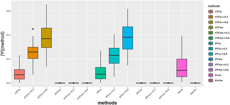
Figure 1. Distribution of absolute partial correlation values, ||Ψ||, for different methods. For G, we used a BA network of size 100. An “e” corresponds to the partial correlation values for edges and “ne” for non-edges.
We would like to emphasize that the algorithm by Kim is parameter free, whereas IPF and HTP depend on a parameter r (see section 2). Interestingly, for IPF/e and HTF/e with r = 0.6 the median partial correlation values are larger than 0.3. In contrast, these methods result for r = 0.0 in median partial correlation values around 0.05. Hence, this parameter allows to influence the correlation strength.
Furthermore, for all three algorithms one can see that the maximal partial correlation values for non-edges are close to zero.
3.2. Global Structure of Covariance Matrices and Influence of Network Structures
Next, we zoom into the structure of the generated covariance matrices and the resulting concentration and partial correlation matrices in more detail. For this reason, we study distances between elements in these matrices. More precisely, we define the following measures to quantify such distances,
Here an “a” means either the algorithm IPF, Kim, or HTF.
The first measure, da(1;Ω), gives the distance between the smallest element in ||Ωa(edges)||I and the largest element in ||Ωa(non-edges)||I, whereas, e.g., ||Ωa(edges)||I corresponds to all elements in the concentration matrix that belong to an edge in the underlying network, as given by G [see the similar definition for the partial correlation matrix in Equations (30, 31)]. That means, formally,
In Figures 2–4 we show results for the algorithms IPF, Kim, and HTF for BA, ER-RN, and WS networks of different sizes, ranging from 25 to 500 nodes. Due to the fact that all three algorithms result in a perfect reconstruction of the underlying networks, as discussed at the beginning of the results section, the entities da(1;Ω), da(2;Ω), da(1;Ψ), and da(2;Ψ) are always positive (as can be seen from the figures).
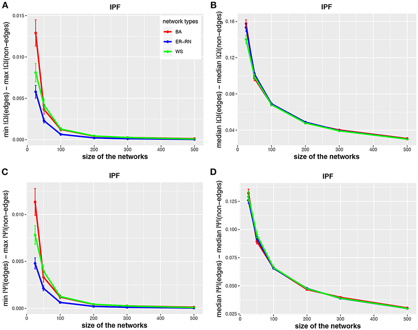
Figure 2. Effect of size differences in the elements of concentration and partial correlation matrices for the IPF algorithm. Shown are differences between values for edges and non-edges in dependence on the network size and network type. All values are averaged over 50 independent runs.
Asymptotically, for large network sizes, the values of the four measures decrease monotonously, except for the Kim algorithm for dKim(2;Ω) (Figure 3B). Furthermore, the structure of the underlying network has for the Kim algorithm a larger influence than for the IPF and HTF algorithms, because the values for dKim(1;Ω) and dKim(2;Ω) do not overlap for the three different network types.
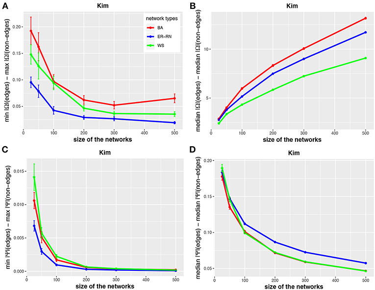
Figure 3. Effect of size differences in the elements of concentration and partial correlation matrices for the Kim algorithm. Shown are differences between values for edges and non-edges in dependence on the network size and network type. All values are averaged over 50 independent runs.
The results from this analysis show clearly that the three algorithms have different working characteristics. First, the IPF and HTF algorithms are only weakly effected by the topology of the underlying network and this effect is even decreasing for larger network sizes; see, e.g., Figures 2, 4. In contrast, the Kim algorithm shows a clear dependency on the network topology, because all three curves for BA, ER-RN, and WS networks are easily distinguishable from each other within, at least, one standard error; see Figure 3. Second, the distances between the median values of the concentration matrix, given by da(2;Ω), show a different behavior, because they are increasing. This is a reflection of the different scale of the elements of the concentration matrix generated by the IPF and HTF algorithm on one side and the Kim algorithm on the other.
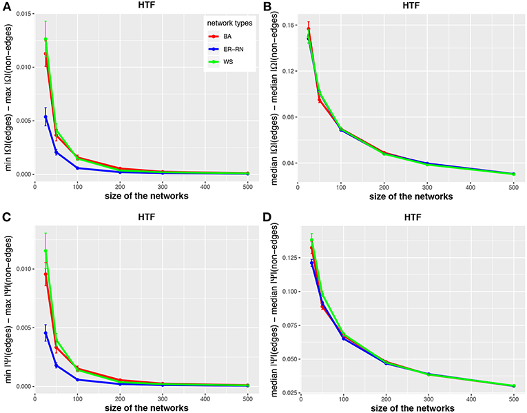
Figure 4. Effect of size differences in the elements of concentration and partial correlation matrices for the HTF algorithm. Shown are differences between values for edges and non-edges in dependence on the network size and network type. All values are averaged over 50 independent runs.
In order to clarify the latter point, we show in Figure 5 the possible range of these values. Specifically, we show normalized results for edges,
as a function of the network size n, i.e., ra(edge, n). The results are normalized, because we divide ra(edge, n) by the maximal value obtained for all studied network sizes, i.e., ra(edge, n)/maxn (ra(edge, n)), to show the curves for all three algorithms in the same figure. One can see that the range of possible values in r(edge, n) increases for the Kim algorithm but decreases for IPF and HTF.
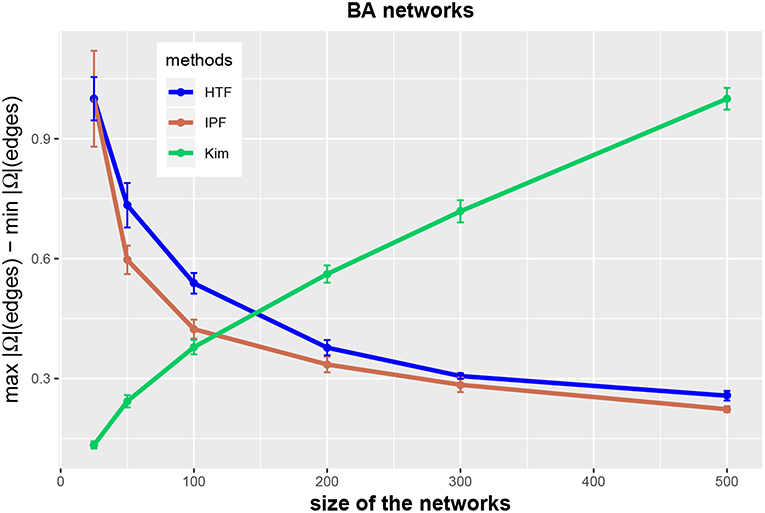
Figure 5. Range of (normalized) values of concentration matrices for the three methods IPF (red), Kim (green), and HTF (blue). All values are averaged over 10 independent runs.
The situation becomes different when one uses values of the control parameter r of the IPF and HTF algorithms that are larger than zero. In order to investigate this quantitatively, we repeat the above analysis for the IPF and HTF algorithm, however, now we set r = 0.3 and r = 0.6. The results of this analysis are shown in Figure 6. The first two columns show results for r = 0.3 whereas the third column presents results for the IFP algorithm for r = 0.6. For these parameters, da(2, Ω) and da(2, Ψ) (see Figures 6D–F,J–L) are nearly constant, even for small network sizes. Furthermore, these distances are much larger than for r = 0.0 (see Figures 2–4). Another difference is that the distances da(1, Ω) and da(1, Ψ) (see Figures 6A–C,G–I) are increasing for increasing sizes of the networks, except for the BA networks (red curves). This indicates also that for r>0 the topology of the underlying network G has a noticeable effect on the resulting concentration and partial correlation matrices, in contrast to the results for r = 0.0 (see Figures 2–4). Overall, the parameter r gives the IPF and HTF algorithms an additional flexibility that allows to increase the observable spectrum of behaviors considerably.
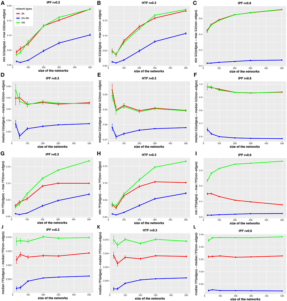
Figure 6. Effect of size differences in the elements of concentration and partial correlation matrices. (A–L) Differences between values for edges and non-edges in dependence on the network size and network type. All values are averaged over 50 independent runs.
3.3. Local Structure of Covariance Matrices and Heterogeneity of Its Elements
Finally, we investigate the local structure of covariance matrices. In Figures 7A–C we show a BA network with 100 nodes. The color of the edges codes the value of the elements of the (normalized) concentration matrices, obtained for IPF, Kim, and HTF. Specifically, we map these values from low to high values to the colors blue, green, and red. From the shown three networks one can see that the coloring is quite different implying a significant difference in the rank order of the elements of the concentration matrices.
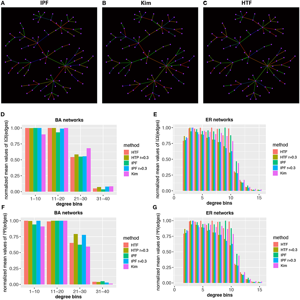
Figure 7. Local structure and heterogeneity of concentraton/partial correlation matrices. Top: In (A–C) estimates of the concentration matrix are shown for a BA network with 100 nodes. The color of the edges corresponds to the value of the elements of the (normalized) concentration matrices, obtained for IPF, Kim, and HTF. The colors blue, green, and red correspond to low, average and high values. Bottom: Normalized mean values of Ω (D,E) and Ψ (F,G) for BA and ER-RN networks of sizes 100. All values are averaged over 50 independent runs.
Next, we study the heterogeneity of the elements in the concentration and partial correlation matrices. More precisely, we are aiming for a quantification of the values of the elements of the concentration/partial correlation matrices that belong to edges with a certain structural property. For reasons of simplicity, we are using the degree (deg) of the nodes that enclose an edge to distinguish edges structurally from each other. Specifically, we calculate for each edge an integer value, v, given by
Here deg(i) is the degree of node i, corresponding to the number of (undirected) connections of this node. This allows us to obtain the expectation value of the concentration/partial correlation elements in a network with a particular value of v, e.g., for v = d,
In Figures 7D–G we show results for BA and ER-RN networks with 100 nodes. The results are averaged over 50 independent runs. For reasons of representability, we normalize the results for the IPF, Kim, and HTF algorithm independently from each other, by division with the maximal values obtain for different network sizes. This allows a representation of all three algorithms in the same histogram, despite the fact that the algorithms result in elements on different scales. Overall, we observe that edges with a higher degree-sum are systematically associated with lower expectation values of the elements of the concentration/partial correlation matrix. Due to the fact that all three algorithms, even for different values of the parameter of r, lead to similar results, our findings hint that this is a generic behavior that does not depend on the underlying network topology or algorithm. In summary, these results reveal a heterogeneity of the values of the concentration/partial correlation matrices.
4. Discussion
4.1. Origin of Inferential Heterogeneity of Gene Regulatory Networks
It is interesting to note that the presented results in Figure 7 follow a similar pattern as results for the inference of gene regulatory networks from gene expression data. More precisely, in previous studies [65–68] it has been found that inferring gene regulatory networks from gene expression data leads to a heterogeneity with respect to the quality (true positive rate) of the inferred edges. That means it has been shown that edges that are connecting genes with a high degree are systematically more difficult to infer than edges connecting genes with a low degree. This has been demonstrated for a number of different popular network inference methods and different data sets and, hence, is method independent [65–68]. In addition, more general structural components of networks have been investigated, e.g., network motifs by using local network-based measures [65, 68]. Also for these measures a heterogeneity in the inferability of edges has been identified.
The important connection between these results and our study is that the results presented in Figures 7D–G provide a theoretical explanation for the heterogeneity in the network inference. In order to understand this connection, we would like to emphasize the double role of the covariance matrix in this context. Suppose, there is a GGM with a multivariate normal distribution given by N(μ, Σ) consistent with a network G. Then, by sampling from this distribution, we create a data set, D(m) = {X1, …, Xm}, with Xi~N(μ, Σ), consisting of m samples. The data set D(m) can then be used for estimating the covariance matrix of the distribution, from which the data have been sampled, resulting in
with . Asymptotically, i.e., for a large number of samples, we clearly obtain
as a converging result.
The double role of the covariance matrix is that it is a (1) population covariance matrix for generating the data, and its is a (2) sample covariance matrix estimated from the data. Both will in the limit coincide, but not in reality when the samples m are finite. For this reason, asymptotically, i.e., for m → ∞, there is no heterogeneity in the inference of edges with respect to the error rate, because, as we saw at the beginning of the results section in this paper, Σ allows a perfect (error free) inference of the network G, due to the fact that Σ is the population covariance matrix of a GGM consistent with G. However, for a finite number of samples this is not the case, as we know from a large number of numerical studies [e.g., [69]] due to the fact that for finite data sets, we will not be able to estimate Σ without errors. Hence, the results of gene regulatory network inference studies mirror the results shown in Figures 7D–G because the decaying normalized mean values of ∥Ω(edges)∥I, respectively ∥Ψ(edges)∥I, are indicative of a decaying signaling strength whereas smaller signals are more difficult to infer in the presence of noise (measurement errors) than larger signals.
Based on the results of our paper (especially those in Figures 7D–G), we can provide an answer to the fundamental question, if the systematic heterogeneity observed for the inference of gene regulatory networks is due to the imperfection of the statistical methods employed for estimating the sample covariance matrix S, or is this systematic heterogeneity already present in the population covariance matrix Σ. Our results provide evidence that the latter is the case because our study did not rely on any particular network inference method. Hence, this provides a probabilistic explanation for the statistical observations from numerical studies.
4.2. Computation Times
Finally, we present information about the time it takes to generate constrained covariance matrices that are consistent with a given graph structure. The following execution times have been obtained with a 1.6 GHz Intel Core i5 processor with 8 GB RAM.
In Table 1, we show the execution time for the algorithms IPF, Kim, and HTF. We would like to emphasize that the shown execution times refer only to the generation of one constrained covariance matrix and do not include any other analysis component. One can see that there are large differences between the three algorithms and HTF is considerable faster than the other algorithms. For instance, for generating a constrained covariance matrix of dimension m = 500, HTF is almost 12-times faster than Kim and 3-times faster than IPF.
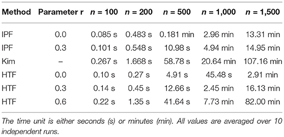
Table 1. Average computation times for the algorithms IPF, Kim, and HTF.
The parameter r has also an influence on the execution time. For instance, for HTF it takes 2.6-times longer to generate a constrained covariance matrix of dimension m = 500 with r = 0.3 than with r = 0.0. For r = 0.6 this effect is even increased by a further factor of 3.5. Hence, utilizing the additional flexibility of this parameter increases the computation times significantly.
In summary, the three simulation algorithms are sufficiently fast to study problems up to a dimension of D ~ O(103−104). Considering that essentially all simulation studies for the inference of gene regulatory networks are performed for such dimensions, e.g., [70–72], because it has been realized that such network sizes are sufficient in order to study the ocurring problems in high-dimensions, all three algorithms can be used for this analysis.
Beyond this application domain, it is interesting to note that also in general GGM are numerically studied up to a dimension of D ~ O(103−104), see e.g., [73, 74]. Hence, for essentially all application domains the three algorithms can be used to study high-dimensional problems but the HTF algorithm could be favored for reason of computational efficiency.
5. Conclusion
In this paper, we investigated three different methods for generating constrained covariance matrices. Overall, we found that all methods generate covariance matrices that are consistent with a given network structure, containing all independence relations among the variables. For a parameter of r = 0.0 for the IPF and HTF algorithms, we found that the Kim algorithm leads to favorable results. However, for r>0 for the IPF and HTF algorithms, these two methods are resulting in a broader spectrum of possible distributions that is considerably larger than that of the Kim algorithm. This extra flexibility could be an advantage for simulation studies.
Regarding computation times of the algorithms, we found that KIM performs slowest. For the IPF algorithm the execution times can be extended due to some outliers that can considerably slow down the execution. The HTF and IPF algorithm perform similarly with slight advantages for HTF, which is overall fastest. Taken together, the HTF algorithm is the most flexible and fastest algorithm that should be the preferred choice for applications.
Aside from the technical comparisons, we found that the generated concentration and partial correlation matrices possess a systemic heterogeneity, independent of the algorithm and the underlying network structure used to provide the independence relations, which is similar to the well-known systematic heterogeneity in studies inferring gene regulatory networks via employing statistical estimators for the covariance matrix [65–67]. Hence, the empirically observed higher error rates for molecular interactions connecting genes with a high node-degree seem not due to deficiencies of the inference methods but the smaller signaling strength in such interactions, as measured by the components of the concentration matrix (Ω) or the partial correlation matrix (Ψ). The implication from this finding is that perturbation experiments are required, instead of novel inference methods, to transform an interaction network into a more amenable form that can be measured. To accomplish this, the simulation algorithms studied in this paper could be utilized for setting up an efficient experimental analysis design.
Author Contributions
FE-S conceived this study. FE-S and ST performed the analysis. FE-S, ST, and MD wrote the paper. All authors proved the final version of the manuscript.
Funding
MD thanks the Austrian Science Funds for supporting this work (project P 30031).
Conflict of Interest Statement
The authors declare that the research was conducted in the absence of any commercial or financial relationships that could be construed as a potential conflict of interest.
Acknowledgments
We would like to thank Robert Castelo and Ricardo de Matos Simoes for fruitful discussions.
References
1. Lander ES. The new genomics: global views of biology. Science. (1996) 274:536–9. doi: 10.1126/science.274.5287.536
2. Nicholson J. Global systems biology, personalized medicine and molecular epidemiology. Mol Syst Biol. (2006) 2:52. doi: 10.1038/msb4100095
3. Quackenbush J. The Human Genome: The Book of Essential Knowledge. Curiosity Guides. New York, NY: Imagine Publishing (2011).
4. Beadle GW, Tatum EL. Genetic control of biochemical reactions in neurospora. Proc Natl Acad Sci USA. (1941) 27:499–506. doi: 10.1073/pnas.27.11.499
5. Dehmer M, Emmert-Streib F, Graber A, Salvador A. (Eds.) Applied Statistics for Network Biology: Methods for Systems Biology. Weinheim: Wiley-Blackwell (2011).
6. Ma H, Goryanin I. Human metabolic network reconstruction and its impact on drug discovery and development. Drug Discov Today. (2008) 13:402–8. doi: 10.1016/j.drudis.2008.02.002
8. Emmert-Streib F, Dehmer M. Information processing in the transcriptional regulatory network of yeast: Functional robustness. BMC Syst Biol. (2009) 3:35. doi: 10.1186/1752-0509-3-35
9. Wang Z, Gerstein M, Snyder M. RNA-Seq: a revolutionary tool for transcriptomics. Nat Rev Genet. (2009) 10:57–63. doi: 10.1038/nrg2484
10. Yates J. Mass spectral analysis in proteomics. Annu Rev Biophys Biomol Struct. (2004) 33:297–316. doi: 10.1146/annurev.biophys.33.111502.082538
11. Tripathi S, Emmert-Streib F. Assessment method for a power analysis to identify differentially expressed pathways. PLoS ONE. (2012) 7:e37510. doi: 10.1371/journal.pone.0037510
12. Qiu X, Klebanov L, Yakovlev A. Correlation between gene expression levels and limitations of the empirical bayes methodology for finding differentially expressed genes. Stat Appl Genet Mol Biol. (2005) 4:35. doi: 10.2202/1544-6115.1157
13. Qiu X, Brooks A, Klebanov L, Yakovlev A. The effects of normalization on the correlation structure of microarray data. BMC Bioinform. (2005) 6:120. doi: 10.1186/1471-2105-6-120
14. Alon U. An Introduction to Systems Biology: Design Principles of Biological Circuits. Boca Raton, FL: Chapman & Hall/CRC (2006).
15. Emmert-Streib F, Dehmer M. Networks for systems biology: conceptual connection of data and function. IET Syst Biol. (2011) 5:185. doi: 10.1049/iet-syb.2010.0025
16. de Matos Simoes R, Dehmer M, Emmert-Streib F. Interfacing cellular networks of S. cerevisiae and E. coli: connecting dynamic and genetic information. BMC Genomics (2013) 14:324. doi: 10.1186/1471-2164-14-324
17. Emmert-Streib F, Dehmer M, Haibe-Kains B. Untangling statistical and biological models to understand network inference: the need for a genomics network ontology. Front Genet. (2014) 5:299. doi: 10.3389/fgene.2014.00299
18. Jeong H, Tombor B, Albert R, Olivai Z, Barabasi A. The large-scale organization of metabolic networks. Nature. (2000) 407:651–4. doi: 10.1038/35036627
20. Yu H, Braun P, Yildirim MA, Lemmens I, Venkatesan K, Sahalie J, et al. High-quality binary protein interaction map of the yeast interactome network. Science. (2008) 322:104–10. doi: 10.1126/science.1158684
21. Ackermann M, Strimmer K. A general modular framework for gene set enrichment analysis. BMC Bioinform. (2009) 10:47. doi: 10.1186/1471-2105-10-47
22. Efron B, Tibshiran R. On testing the significance of sets of genes. Ann Appl Stat. (2007) 1:107–29. doi: 10.1214/07-AOAS101
23. Glazko G, Emmert-Streib F. Unite and conquer: univariate and multivariate approaches for finding differentially expressed gene sets. Bioinformatics. (2009) 25:2348–54. doi: 10.1093/bioinformatics/btp406
24. Giles PJ, Kipling D. Normality of oligonucleotide microarray data and implications for parametric statistical analyses. Bioinformatics. (2003) 19:2254–62. doi: 10.1093/bioinformatics/btg311
26. Shahbaba B. Biostatistics with R: An Introduction to Statistics Through Biological Data. Use R!. New York, NY: Springer New York (2011).
27. de Matos Simoes R, Tripathi S, Emmert-Streib F. Organizational structure of the peripheral gene regulatory network in B-cell lymphoma. BMC Syst Biol. (2012) 6:38. doi: 10.1186/1752-0509-6-38
28. de Matos Simoes R, Emmert-Streib F. Bagging statistical network inference from large-scale gene expression data. PLoS ONE. (2012) 7:e33624. doi: 10.1371/journal.pone.0033624
29. Albert R. Scale-free networks in cell biology. J Cell Sci. (2005) 118:4947–57. doi: 10.1242/jcs.02714
30. van Noort V, Snel B, Huymen MA. The yeast coexpression network has a small-world, scale-free architecture and can be explained by a simple model. EMBO Rep. (2004) 5:280–4. doi: 10.1038/sj.embor.7400090
31. Van den Bulcke T, Van Leemput K, Naudts B, van Remortel P, Ma H, Verschoren A, et al. SynTReN: a generator of synthetic gene expression data for design and analysis of structure learning algorithms. BMC Bioinform. (2006) 7:43. doi: 10.1186/1471-2105-7-43
32. Tripathi S, Lloyd-Price J, Ribeiro A, Yli-Harja O, Dehmer M, Emmert-Streib F. sgnesR: an R package for simulating gene expression data from an underlying real gene network structure considering delay parameters. BMC Bioinform. (2017) 18:325. doi: 10.1186/s12859-017-1731-8
35. Castelo R, Roverato A. Reverse engineering molecular regulatory networks from microarray data with qp-graphs. J Comput Biol. (2009) 16:213–27. doi: 10.1089/cmb.2008.08TT
36. Emmert-Streib F. Influence of the experimental design of gene expression studies on the inference of gene regulatory networks: environmental factors. PeerJ. (2013) 1:e10. doi: 10.7717/peerj.10
37. Kim KI, van de Wiel M. Effects of dependence in high-dimensional multiple testing problems. BMC Bioinform. (2008) 9:114. doi: 10.1186/1471-2105-9-114
38. Speed T, Kiiveri H. Gaussian markov distributions over finite graphs. Ann Stat. (1986) 14:138–50. doi: 10.1214/aos/1176349846
39. Haste T, Tibshirani R, Friedman J. The Elements of Statistical Learning: Data Mining, Inference and Prediction. New York, NY: Springer (2009).
40. Dudoit S, Shaffer J, Boldrick J. Multiple hypothesis testing in microarray experiments. Stat Sci. (2003) 18:71–103. doi: 10.1214/ss/1056397487
41. Goeman J, Buhlmann P. Analyzing gene expression data in terms of gene sets: methodological issues. Bioinformatics. (2007) 23:980–7. doi: 10.1093/bioinformatics/btm051
42. Rahmatallah Y, Emmert-Streib F, Glazko G. Gene set analysis for self-contained tests: complex null and specific alternative hypotheses. Bioinformatics. (2012) 28:3073–80. doi: 10.1093/bioinformatics/bts579
43. Rahmatallah Y, Zybailov B, Emmert-Streib F, Glazko G. GSAR: bioconductor package for gene set analysis in R. BMC Bioinform. (2017) 18:61. doi: 10.1186/s12859-017-1482-6
44. Hartemink AJ. Reverse engineering gene regulatory networks. Nat Biotechnol. (2005) 23:554. doi: 10.1038/nbt0505-554
45. Emmert-Streib F, de Matos Simoes R, Glazko G, McDade S, Haibe-Kains B, Holzinger A, et al. Functional and genetic analysis of the colon cancer network. BMC Bioinform. (2014) 15:6. doi: 10.1186/1471-2105-15-S6-S6
46. Whittaker J. Graphical Models in Applied Multivariate Statistics. Chichester: John Wiley & Sons (1990).
47. Spirtes P, Glymour C, Scheines R. Causation, Prediction, and Search. New York, NY: Springer (1993).
48. Castelo R. A robust procedure for gaussian graphical model search from microarray data with p larger than n. J Mach Learn Res. (2006) 7:2621–50. Available online at: http://www.jmlr.org/papers/v7/castelo06a.html
49. Fujikoshi Y, Ulyanov V, Shimizu R. Multivariate Statistics: High-Dimensional and Large-Sample Approximations. New York, NY: Wiley (2011).
51. Smith W, Hocking R. Algorithm AS 53: Wishart variate generator. J Royal Stat Soc Ser C Appl Stat. (1972) 21:341–5.
52. Bornholdt S, Schuster H. (Eds.) (2003). Handbook of Graphs and Networks: From the Genome to the Internet. Weinheim: Wiley-VCH.
53. Emmert-Streib F. A brief introduction to complex networks and their analysis. In: Dehmer M, editor. Structural Analysis of Networks. Boston, MA: Birkhäuser Publishing (2010). p. 1–26.
58. Solomonoff R, Rapoport A. Connectivity of random nets. Bull Math Biophys. (1951) 13:107–17. doi: 10.1007/BF02478357
60. Watts D. Small Worlds: The Dynamics of Networks between Order and Randomness. Princeton, NJ: Princeton University Press (1999).
61. Dehmer M, Emmert-Streib F. (Eds.) Analysis of Complex Networks: From Biology to Linguistics. Weinheim: Wiley-VCH (2009).
62. R Development Core Team. R: A Language and Environment for Statistical Computing. Vienna: R Foundation for Statistical Computing (2008).
63. Csardi G, Nepusz T. The igraph software package for complex network research. Inter J Complex Syst. (2006) 1695:1–9. Available online at: http://igraph.org
64. Tripathi S, Dehmer M, Emmert-Streib F. NetBioV: an R package for visualizing large-scale data in network biology. Bioinformatics. (2014) 30:384. doi: 10.1093/bioinformatics/btu384
65. Altay G, Emmert-Streib F. Revealing differences in gene network inference algorithms on the network-level by ensemble methods. Bioinformatics (2010) 26:1738–44. doi: 10.1093/bioinformatics/btq259
66. Altay G, Emmert-Streib F. Structural Influence of gene networks on their inference: analysis of C3NET. Biol Direct. (2011) 6:31. doi: 10.1186/1745-6150-6-31
67. de Matos Simoes R, Emmert-Streib F. Influence of statistical estimators of mutual information and data heterogeneity on the inference of gene regulatory networks. PLoS ONE. (2011) 6:e29279. doi: 10.1371/journal.pone.0029279
68. Emmert-Streib F, Altay G. Local network-based measures to assess the inferability of different regulatory networks. IET Syst Biol. (2010) 4:277–88. doi: 10.1049/iet-syb.2010.0028
69. Emmert-Streib F, Glazko G, Altay G, de Matos Simoes R. Statistical inference and reverse engineering of gene regulatory networks from observational expression data. Front Genet. (2012) 3:8. doi: 10.3389/fgene.2012.00008
70. He B, Tan K. Understanding transcriptional regulatory networks using computational models. Curr Opin Genet Dev. (2016) 37:101–8. doi: 10.1016/j.gde.2016.02.002
71. Margolin A, Nemenman I, Basso K, Wiggins C, Stolovitzky G, Favera RD, et al. ARACNE: an algorithm for the reconstruction of gene regulatory networks in a mammalian cellular context. BMC Bioinform. (2006) 7:S7. doi: 10.1186/1471-2105-7-S1-S7
72. Werhli A, Grzegorczyk M, Husmeier D. Comparative evaluation of reverse engineering gene regulatory networks with relevance networks, graphical gaussian models and bayesian networks. Bioinformatics. (2006) 22:2523–31. doi: 10.1093/bioinformatics/btl391
73. Liu H, Han F, Yuan M, Lafferty J, Wasserman L. High-dimensional semiparametric gaussian copula graphical models. Ann Stat. (2012) 40:2293–326. doi: 10.1214/12-AOS1037
Keywords: Gaussian graphical models, network science, machine learning, data science, genomics, gene regulatory networks, statistics
Citation: Emmert-Streib F, Tripathi S and Dehmer M (2019) Constrained Covariance Matrices With a Biologically Realistic Structure: Comparison of Methods for Generating High-Dimensional Gaussian Graphical Models. Front. Appl. Math. Stat. 5:17. doi: 10.3389/fams.2019.00017
Received: 27 July 2018; Accepted: 22 March 2019;
Published: 12 April 2019.
Edited by:
Xiaogang Wu, University of Nevada, Las Vegas, United StatesReviewed by:
Maria Suarez-Diez, Wageningen University & Research, NetherlandsEdoardo Saccenti, Wageningen University & Research, Netherlands
Copyright © 2019 Emmert-Streib, Tripathi and Dehmer. This is an open-access article distributed under the terms of the Creative Commons Attribution License (CC BY). The use, distribution or reproduction in other forums is permitted, provided the original author(s) and the copyright owner(s) are credited and that the original publication in this journal is cited, in accordance with accepted academic practice. No use, distribution or reproduction is permitted which does not comply with these terms.
*Correspondence: Frank Emmert-Streib, v@bio-complexity.com