Introduction
The Lambert Glacier basin system occupies almost 1000 000km2 between eastern Kemp Land and western Princess Elizabeth Land from 55°–80°E draining around one-eighth of the Last Antarctic ice sheet. The Lambert Amery Regional Glaciological Experiment (LARGE), conducted for the Antarctic Division by the Australian National Antarctic Research Expeditions (ANARE), operated a series of oversnow traverses from 1989 to 1995 in order to investigate the dynamics and mass budget of the basin. The mass budget has been estimated in the past from extrapolation of isolated measurements Reference AllisonAllison, 1979 and interpretation of satellite imagery (Reference McIntyreMcIntyre, 1985), offering alternative descriptions of the current state of balance.
Initial results from LARGE confirmed indications (Reference Giovinetto and BullGiovinetto and Bull, 1987) that the western coastal sector of the basin receives low accumulation (<150kg m−2 a−1 with variability of about 50% independent of elevation or Continentality (Reference Goodwin, Higham, Allison and JaiwenGoodwin and others, 1994). Results for the entire route demonstrate some elevation and continentality effects over the western and southern extremities, continued high variability indicative of surface snow redistributed by a strong wind regime, and lower accumulation rates at equivalent altitudes for the eastern sector of the basin.
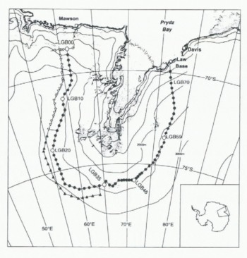
The traverse program established a series of ice-movement stations, for GPS satellite determination of ice-sheet velocities, at 30 km intervals along more than 2000km of track (Fig. 1). Double-tagged bamboo canes were spaced every 2 km along the entire route to aid navigation and facilitate measurement of spatial and temporal (western sector variability in annual snow accumulation. At each station 10 m firn temperatures were recorded and shallow 2 m cores were drilled for measurements of density, Stratigraphy and isotope analysis studies of climatological aspects of the precipitation. At seven selected stations, cane farms consisting of 20–25 canes at 200m intervals in square or crossed arrays with axes parallel and perpendicular to prevailing winds; were established in order to determine accumulation dependence on small-scale topography and local-surface microrelief. All but one (LGB68) coincide with automatic weather stations (AWS), spaced at roughly 300 km intervals around the basin, which routinely relayed remoter) sampled meteorological data. Shallow cores were drilled to depths of 15–60 m at 15 selected sites around the basin for stratigraphic studies of annual layers and analysis of grain-sizes within the firn.
Fig. 1. Map of the Lambert Glacier basin (Antarctic location inset) and LARGE operational area 1989–95, showing AWS (open circles), main traverse route and stations (dark circle), offset lines (triangle) and short western route (diamonds).
The route follows a nearly constant elevation along the 2500 m contour where surface slopes and wind speeds are typical of the katabatic zone. The low surface mass balance gives the near-surface firn different characteristics from those found for a given elevation in many other parts of East Antarctica (Reference Goodwin, Higham, Allison and JaiwenGoodwin and others, 1994). An understanding of the dependence of firn properties on accumulation rates can be used in the interpretation of remotely sensed data covering the entire drainage basin.
Surface Mass Balance
Measurement Techniques
Measurements of surface mass balance were made on 989 bamboo canes spaced at 2 km intervals, with accuracy estimated to be ±20 mm absolute, over 2014 km of traverse route at surface elevations up to 3000 m (Table 1). For each period, annual mass-balance values have been calculated assuming no seasonal variability. Surface net-accumulation distributions derived from atmospheric-moisture fluxes show relatively little systematic variation during the year for inland regions above 1500 m (Reference Budd and Reid MintyBudd and others, 1995).
Table 1. Periods of accumulation data over portions of the traverse route

Measurements of surface snow density along the traverse route were obtained from an average value for the upper metre of a shallow core collected every 2 km. This includes the windpacked surface plus snow undergoing firnfication with associated density changes. Values range from 480kgm−3 under the strong katabatic effect on the near-coastal slopes, to a low of 360kgm−3 along the southern part of the route due to shallow depth hoar development, with an overall average of 408 kg m−3.
Accumulation Regimes
The spatial variation of snow accumulation around the basin is plotted with ice surface elevation against distance in Figure 2. The broadscale topography is undulating on a wavelength of approximately 350 km over the western half of the basin, changing in character to around 150 km wavelength across the southeastern portion of the route up to LGB61, from where the surface elevation begins a steady decline toward the coast. The accumulation data have been smoothed over 30 km (15 canes) using an unweighted running mean and have been converted to mass using near-surface density measurements. Smoothing removes high frequency fluctuations that are due to local effects, but the consequences of large-scale features remain. Standard deviations, exhibiting strong anti-correlation with accumulation, have been determined for each 30 km interval and are shown divided by the mean as coefficients of variation in Figure 2.
Fig. 2. Surfacee elevations (mst) along the traverse route (top), including the first 500 km of western offset line, plotted against 1994 accumulation figures (middle) and the coefficient of variation (bottom). The large peak around 130 km has a value of 6.4, due to the very low accumulation near the break in coastal slope.
The basin can be divided into three main accumulation regimes: the western sector from LGB06 to LGB29 with an annual 1994 mean accumulation of 94 kg m−2 a−1 (σ = 74); the southern sector from LGB29 to LGB50, 56 kg m−2 a−1(σ = 72); and the eastern sector from LGB50 to LGB67, 70kg m−2 a−1 (σ = 71). The standard deviations have similar absolute values, with magnitudes close to the mean within each zone, indicating that they represent the average surface microrelief contribution to variability. Stratigraphic analysis of shallow firn-core samples (15–60 m) has failed to yield reliable accumulation-rate time series due to masking of the annual layering by acolian processes driving surface microrelief features of similar magnitude and the occurrence of depth-hoar metamorphism, tending to further confuse identification of strata.
The low accumulation figure across the southern portion of the route is a reflection of continentality superimposed on a small elevation trend, whilst lower accumulation on the eastern sector compared to that at equivalent altitude on the western sector is a function of the surface-wind regime and ice-sheet gradients across the basin. This rain-shadow effect is consistent with observations of higher accumulation rates on windward compared to leeward slopes in Wilkes Land for elevations around 2000 m. (Reference GoodwinGoodwin, 1990). Scattergrams of accumulation vs elevation show a small dependence superimposed on large variability for the western and southern sectors, with no evidence for dependence on the eastern side (Fig. 4). This indicates an eastern sector where accumulation is controlled by topographic features with the amount of enhancement in the valleys dependent on localised gradients rather than absolute elevation.

Fig. 4. Elevation scattergrams for the accumulation regimes in the Lambert basin (top). The eastern sector (circles) shows no dependence on elevation. The 10m firn temperatures vs elevation plots (bottom) depict lapse rates that are slightly Superadiabatic for the eastern and western (triangles) sectors.
Repeat measurements from LGB00 to LGB16 give an indication of the temporal variability of the annual net-surface balance for the region (Fig. 3). Of particular interest are the low accumulation record for 1993 and the high for 1990.1993 was the second coldest year at Mawson since station records began in 1955 (a mean annual temperature of −13°C compared to the long term 39 year mean of −11.2°C). Average accumulation over the 504 km from LGB00 to LGB16 was 56 kg in m−2a−1 (σ = 76), half the 5 year average for the area. For 1990 the average was 131 kgm−2 a−1 (σ = 104) whilst the mean temperature was close to average at −10.8°C, the larger standard deviation perhaps indicative of increased microrelief features, particularly on the break in slope around the ridge line near LGB05 and a smaller gradient change on the southern extremity of the valley running across the route between LGB10 to LGB14. April-May temperatures were, however, some 3–4°C above the long-term averages, indicating possible intrusion of moisture-laden air during the early phase of sea-ice formation, resulting in heavier snowfall through this period. This could indicate possible seasonality in the accumulation pattern, which has, however, not been included in the calculations for balance years. The high variability emphasises the need for accumulation measurements to be carried out over periods of at least 3–4 years. The 1994 accumulation record Mawson mean temperature of −11.5°C) was Consistent with the 5 year average (93 kg m−2 a −1 (σ = 74) vs 101 kgm−2 a−1 (σ = 81), most of the discrepancy accounted for over the first 150 km of steep coastal slope) increasing confidence in the figures recorded for one season only over the eastern sector.

Fig. 3. Inter-annual variability from LGB00 to LGB16 shown in terms of percentage residuals for individual periods (bottom) from the 1990–945 year mean (top).
Cane farms were established ai approximately 300 km intervals along the route to facilitate investigation of small-scale spatial variability. Even for very low accumulation (LGB35, 1994) the standard deviation remains around 30kgm−2 a−1, indicating a possible lower limit to average local microrelief size (Table 2). This corresponds to about half the standard deviation found over the entire traverse route (70 kgm−2 a−1).
Table 2. Caue farms. (n = number of canes,
![]() = mean annual accumulation in kg m−2
a−1, σ = standard deviation and numbers in the bottom
row are overall averages)
= mean annual accumulation in kg m−2
a−1, σ = standard deviation and numbers in the bottom
row are overall averages)
Cane-farm averages and track canes compare favourably. For example, LGB10, where the cane-farm average was 122 kgm−2 a−1 (σ = 40), the station cane over the same 5 year period (1990–91) recorded 145 kgm−2 a−1, while the 30 km (15 canes) smoothed value along the track in the vicinity of LGB10 was 132 kgm−2 a−1 (σ = 54). This implies that the variability in the accumulation signal over a 30 km interval is mostly accounted for by noise introduced from microrelief processes. The corollary to this is that modification of the signal (at the 2 km sampling frequency) mesoscale topography occurs over distances significantly greater then 30 km.
Temperature and Wind Regimes
The 10 m firn temperature has been measured at all stations using a platinum resistance thermometer in a hole, steam drilled one year and measured the next (Fig. 4). Across the southern sector the lapse rate, −0.8°C 100m−1 (r2 = 0.84), lies midway between dry and moist adiabatic values. For the western sector it has a superadiabatic value of −1.4°C 100m−1 (r2 = 0.90), with a similar result along the eastern sector transition stations LGB51 and LGB52 removed from the dataset) of 1.−3°C 100m −1 (r2 = 0.95). Mean temperatures are some 4°C colder at equivalent elevations on the western sector as a consequence of transport of cooler air from higher elevations to the south. Overall values reflect differences in surface slopes and local surface wind regime consistent with topographical lapse rates discussed elsewhere (Reference Allison, Wendler and RadokAllison and others, 1993).
Automatic weather stations (AWS) were deployed at all cane-farm sites apart from LGB68. Annual mean temperatures at these sites are in accord with 10m firn measurements. Sastrugi orientations agree well with wind-direction data interpolated between AWS sites, apart from the southwest sector of the basin from LGB18 to LGB25 (Fig. 5), where reshuffled surfaces of large vertical extent dominate. AWS data indicate a variability of ±20° clockwise from the mean wind direction from autumn to spring at LGB20, maintaining production of microrelief features as opposed to continual erosion from more constant wind directions in other parts of the basin. Interpolated mean-surface winds are oriented some 20 to the left of the fall line (personal communication from H. Phillips, 1996) along the eastern portion of the basin, increasing to 60 from the southeast corner around the western sector, where down-slope katabatic winds with eastward aspect are deflected by an easterly geostrophic-wind regime.
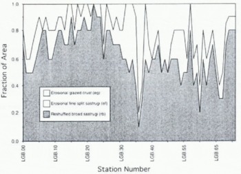
Fig. 5. Distribution of microrelief around the traverse route depicting a high predominance of reshuffled surface types, particularly for the western sector, with strong glazing evident near LGB35 along the southernmost portion of the route.
The western side of the basin is characterised by high proportions of reshuffled drift snow forming banks, dunes and juvenile lanceolate sastrugi (Reference GoodwinGoodwin type rb, 1990), with generally 70% or more arcal coverage (Fig. 6). This peaks at 100% around LGB20, where the cane farm shows consistently high standard deviations from the mean. Sastrugi heights average 0.5 m in this region. Strongly glazed surfaces approach 80% coverage to the east of LGB35, varying between 20 and 60% along the undulating eastern sector of the route, maximising on local topographic highs. AWS data indicate strongest winds at either end of the traverse route, where coastal slopes are greatest, and at LGB35, where the valley effect of upstream extensions of the Lambert and Mellor Glaciers again increase surface gradients in a region characterised by a higher fraction of glazed surface area.
Fig. 6. Sastrugi orientation, wind interpolated from six AWS sites and fall-line Calculated from a preliminary DEM (personal communication Jivmfrom H. Phillips) for the basin. Note the sharp change in fall-line direction from LGB00-05 down the sleep coastal slope, to LGB06 over the ridge where flow into the basin proper commences.
A Revised Accumulation Distribution for the Lambert Basin
Mass-budget estimates for the Lambert basin have reported widely varying results, largely due to differences in proposed average-accumulation rates for the interior basin. Reference McIntyreMcIntyre (1985) interpreted Landsat images as depicting a large ablation zone across the southern sector of the traverse route. Station LGB35 is situated on the southwestern extremity of the proposed zone where a series of heavily crevassed ice domes feature over the next 100km. Average winter winds (AWW) of 12 m s−1, more typical of the coastal slopes to the north, convert the surface over much of this area into wind-glazed crust (80% coverage in places with a mixture of small erosional and reshuffled sastrugi). No bare-ice areas were evident in the region along the traverse route, which weaved a path north and south of the general east west trend to avoid heavily crevassed areas. Measurements show this zone to be a low-accumulation region, 57 kgm−2 a −1 (σ = 69), associated with appreciable depth-hoar formation.
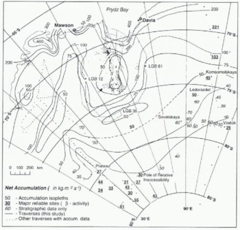
The surface mass-balance distribution for the Lambert basin (Fig. 7) has been revised using the latest compilation of accumulation data from the extensive traverse observations and spot values obtained in the interior (Reference Kotlyakov, Barkov, Loseva and PetrovKotlyakov and others, 1974). Close to the southwest perimeter of the basin reliable data on accumulation rate is available for the Pole of Relative Inaccessibility (82°07’S, 55°02’E, 3718m), Plateau Station (79°1.5’S, 40°30’E,3624 m) and from traverses covering this region (Reference Koerner and CraryKoerner, 1971; Reference Picciotto, Cameron, Crozaz, Deutsch and WilgainPicciotto and others, 1968) using the peak in β activity to define the 1955 annual layer. Although a number of Russian traverses have covered the southeast perimeter, their data are based upon the less reliable stratigraphic interpretation of snow pits, (Reference Kotlyakov and LyubaretsKotlyakov and others, 1966). The nearest sites to this portion of the basin with reliable accumulation from β activity are Vostok (78°29’S 105°30’E, 3190 m), Komsomolskaya (74°05’S 97°29’ E, 1500 m) and Ledorazdel (75°55’S 94°04’E, 3730 m) (see Reference Vinogradov and LoriusVinogradov and Lorius, 1971). Annual accumulation rates obtained at Komsomolskaya, Vostok and on the South Pole-Dronning Maud Land traverses (1964–68) by the stratigraphic interpretation of snow pits were found to be often over-estimated when compared to that obtained from the distribution of gross β activit) (Reference Koerner and CraryKoerner, 1971; Reference Picciotto, Crozaz, de Breuck and CraryPicciotto and others, 1971; Reference Endo and FujiwaraEndo and Fujiwara, 1973). On the western side of the basin (40–50°E) net accumulation has been obtained from snow stakes and stratigraphic interpretation of snow pits and shallow cores on the Japanese traverses (Reference Endo and FujiwaraEndo and Fujiwara, 1973; Reference Yamada and WatanabeYamada and Watanabe, 1978; Reference Satow, Nishimura and InoueSatow and others, 1983; Reference Takahashi, Ageta, Fujii and WatanabeTakahashi and others, 1994).
Fig. 7. New accumulation distribution for the Lambert Glacier basin. The isolated 50 kgm−2 a−1 isolated at 76° S is interpreted to match observed wind-glazed surfaces in the vicinity of LGB35.
At Vostok, Pole of Inaccessibility and Plateau stations, and for some of the intervening traverses, there is similar continentality and elevation. At these localities the mean accumulation rale accurately determined from β activity was 25–30kgm−2a−1. At Komsomolskaya and Ledorazdel, which are closer in the coast, accumulation rate was 45–50kgm−2a−1. The value of 60kgm−2 a−1 for accumulation measured al Sovclskaya (78°23’ S, 87°32’ E, 3662 m) is rather high when compared to these and other neighbouring regions of similar situation. Although this value was obtained from the average of a large number of stakes over the period 1958–61, and it compares well with that obtained from snow-pit stratigraphy for the period 1952–61, it is possible that it has been subjected to a number of undue influences. Reference Vinogradov and LoriusVinogradov and Lorius (1971) attribute higher accumulation at Vostok and Pionerskaya stations during the earlier studies to disturbances caused by proximity of the stake farms to station buildings Nuddman, 1966, photograph p.97. The value may also be influenced by the high rate of accumulation during this period, in particular during 1959. Unfortunately, the use of β activity to identify the mean rate of accumulation is not available for Sovetskaya, and the given value is treated with caution. In any case, such a large value is regarded here as being not representative of the temporal and spatial mean applicable to the neighbouring portion of the inland Lambert basin.
No data are available for the extensive central inland basin region (beyond the 50 kg−2 m a−1 isopleth), but by interpolation with the inland sites the areal mean is estimated to be approximately 39–54 kg m−2 a−1.
Conclusions
Spalial accumulation rates around the Lambert Glacier basin catchment area over an elevation range 2000–3000m are significantly lower than those for similar elevations in other pans of East Antarctica. For example Wilkes Land. The southern portion of the basin, around 76°S, shows distinct continentality effects with firm wind-glazed surfaces and depth-hoar formation characteristic of a low-accumulation regime. No bare-ice areas were found in the vicinity of the traverse route along this latitude. Accumulation rates on the eastern side of the basin are lower than those at equivalent altitudes along the western sector as a result of dominant southeasterly wind fields under the combined influence of katabatic and geostrophic flows. Whilst initial stratigraphic investigations have provided largelv ambiguous records, long-term average accumulation rates may still lie obtainable using absolute datable horizons and characteristic firnification processes from shallow cores collected at various sites round the basin. A new accumulation distribution has been derived for the Lambert basin down to the 30 kg m−2 a−1 isopleth.
Acknowledgements
The authors wish to acknowledge the support of all ANARE and Australian Antarctic Division personnel who have assisted with the field-work and preparations for LARGE, in particular R. Kiernan. who played a pivotal role in the traverse program. W. Budd, I. Goodwin and H. Phillips contributed useful discussion regarding modelled wind fields, surface properties and fall lines from a satellite altimeter digital-elevation model for the basin, respectively. Diagrams for the manuscript were prepared by U. Ryan.