
. Introduction
In optically stimulated luminescence (OSL) dating, the burial age of sediments can be estimated by dividing the equivalent dose (De) by the environmental dose rate (D). OSL dating plays a key role in providing chronological frameworks in Quaternary geology, environmental archaeology and studies of paleo-earthquakes and tectonic movements. The single-aliquot regenerative-dose (SAR) procedure for quartz is widely used in measuring the equivalent dose (De) of sediments (Banerjee et al., 2001), but it is time-consuming, especially for measuring old samples with high De values. The establishment of a standardised growth curve (SGC) has the potential to substantially reduce the instrumental time required for OSL dating (Roberts and Duller, 2004). However, the applicability of the SGC method remains controversial, because several studies have suggested that different samples have different dose–response curves (DRCs), and, thus it is difficult to establish a common SGC (Murray and Wintle, 1999a, b; Chen et al., 2001; Stevens et al., 2007; Telfer et al., 2008; Chen et al., 2013). Nevertheless, the SGC method has been widely applied in dating sediments (especially loess) in several regions (Roberts and Duller, 2004; Lai, 2006, 2010; Lai et al., 2007; Long et al., 2010; Yang et al., 2011).
In order to reduce inter-aliquot/inter-sample variation in the form of DRCs, a variety of methods have been developed, including the following: 1) establishing a common growth curve based on the arithmetical average value of the sensitivity-corrected OSL signal (Lx/Tx) for different regenerative doses of six or more aliquots for each sample and then obtaining the De values of additional aliquots by projecting the test-dose-corrected OSL signal on the constructed common growth curve, namely the SAR-SGC method (Lai and Ou 2013). 2) Re-normalisation of the sensitivity-corrected natural signal (Ln/Tn) and regenerative-dose signal (Lx/Tx), respectively, with the OSL signals of a specific regenerative dose (Lr/Tr), which is called the regenerative normalisation or re-normalisation (Re-SGC) method (Li et al., 2015). 3) All of the regenerative-dose signals are considered for normalisation in the establishment of an SGC using a least-squares procedure, as part of an iterative scaling and fitting process, termed the LS-SGC method (Li et al., 2016).
The present study aims to investigate the applicability of the SGC method for the single-aliquot OSL dating of quartz and to establish a potential SGC of quartz fractions from sediments in different sedimentary environments (including lacustrine, fluvial and desert) in the Jilantai Basin in North China, using the three methods mentioned above. The De values obtained using different methods are validated based on a comparison with those obtained using the SAR protocol.
. Study area and samples
The Jilantai Basin is located on the western edge of the East Asian summer monsoon, in the arid–semi-arid transition zone, which is sensitive to climatic and environmental changes. The Yellow River flows through the south-eastern margin of the basin. Previous studies documented a series of ancient lake–shorelines distributed on the west bank of the Jilantai Salt Lake through remote sensing images and field investigations. It is believed that the area once contained the ‘Jilantai-Hetao’ megalake, which covered the entire Jilantai Basin and the adjacent Hetao Basin (Chen et al., 2008) as a result of the inflow of the Yellow River (Fan et al., 2010a). Today, most of the area of the Jilantai Basin is occupied by the Ulan Buh Desert, and only the Jilantai Salt Lake and several sporadic, small salt lakes are preserved in the western part of the area. Fluvial sediments of seasonal rivers and lacustrine sediments are preserved in the forefront of the Helan Mountains and in the north-eastern part of the Jilantai Basin. In recent years, several studies of lake–desert evolution have been carried out in the area, based mainly on OSL dating (e.g. Chen et al., 2008, 2014; Fan et al., 2010b, 2015, 2017; Zhao et al., 2012; Jia et al., 2015). The area is therefore well suited for assessing whether a potential SGC can be established which is suitable for samples from different profiles or sedimentary environments within a single area.
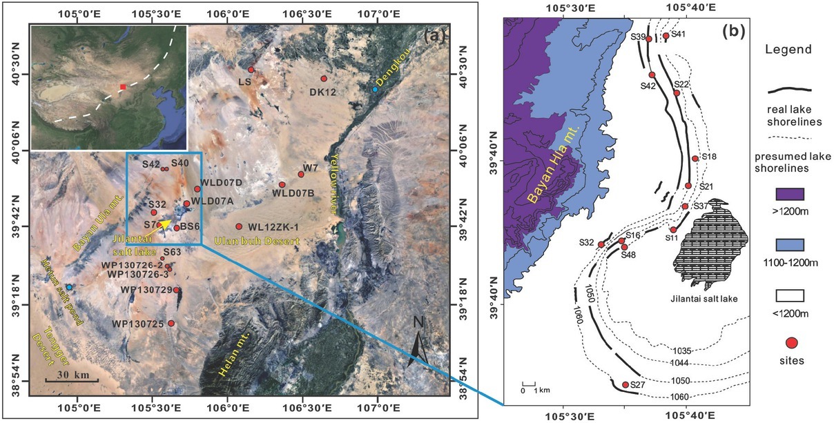
More than 100 quartz samples were used in this study, including lacustrine sediments from 16 profiles, fluvial sediments from 6 profiles and desert sediments from 6 profiles (see Figs. S1–S4 in the supplementary material for details). The location of those profiles is shown in Fig. 1a.
Fig 1
Regional setting (a) and sampling sites (b) (modified from Chen et al., 2008). The inset in the left upper corner of (a) is a remote sensing image of East Asia showing the location of the study area (marked by square) and the modern monsoon limit.
. Methods
Quartz fractions were extracted using conventional separation methods (Fan et al., 2010b). The OSL signals from the extracted quartz fractions were measured using a Risø TL/OSL DA-20 Reader equipped with blue LEDs, infra-red (IR) LEDs and an accurately calibrated 90Sr/90Y beta source, in the Key Laboratory of Western China’s Environmental Systems (Ministry of Education, P.R. China) at Lanzhou University. The purity of the quartz was assessed based on the absence of an infrared-stimulated luminescence signal (IRSL) at a temperature of 50°C prior to measurement of the blue-stimulated luminescence signal. The natural OSL signals and regenerative-dose OSL signals were measured for quartz fractions, which were mounted on 2-mm-diameter small aliquots, using the double SAR procedure (post-IR OSL) (Banerjee et al., 2001) (Table S1). In order to select a suitable preheat temperature, a dose recovery test was performed for each sample. For these aliquots, the natural OSL signals were reset under strong sunlight in Lanzhou (36.04° N, 103.8° E) for more than 6 h, and they were then given a known laboratory dose and the recovered OSL signals measured using the protocol listed in Table S1, with a preheat temperature increasing from 160 to 260°C at 20°C intervals. Only the preheat temperature at which both the recycling ratios and dose recovery ratios (given dose/measured dose) were within the range of 0.9–1.1, and recuperations were <5%, was employed in the protocol to measure the OSL signals. For example, a preheat temperature of 220°C and cut-heat temperature of 160°C were found to be appropriate for equivalent dose measurements of sample S63-2 (Fig. S5 and Table S2 in the supplementary materials). Detailed information on the samples is summarised in Table S2, including geographical locations, depositional environments and the grain size and conditions for measurement of the OSL signals.
The SGC was established using the sensitivity-corrected signal from a wide range of different regenerative doses using the three previously reported methods: SAR-SGC (Lai and Ou, 2013), Re-SGC (Li et al., 2015) and LS-SGC [Li et al., 2016; Peng and Li, 2017). Most of the previous researches have only validated the reliability of aliquots in which OSL signals were involved in establishing the SGC.
However, in this study, in order to investigate whether the constructed SGC is widely applicable to samples from the study area, we classified all of the aliquots into two groups: the OSL signals of aliquots with De values widely distributed in samples of one group were used to establish the SGC, and the OSL signals of aliquots with De values within the range of 200 Gy in another group were used to validate the constructed SGC.
SAR-SGC
The SAR-SGC method is designed to obtain De values from large numbers of aliquots from a single sample, assuming that aliquots of the same sample have similar DRCs. The SGC is constructed by fitting the averaged sensitivity-corrected signals (Lx/Tx) of aliquots with regenerative doses in a single sample. An exponential plus linear function is usually used in curve fitting, and the De values are obtained from the intercept value on the regenerative-dose axis (x-axis) after projecting the sensitivity-corrected natural signal (Ln/Tn) to the SGC. The formula used is as follows:
Here, y is the intensity of the luminescence signal; x is the regenerative dose; a is the normalised OSL intensity at the saturation level for the exponential growth part; D0 is the characteristic dose where the slope of the growth curve (the exponential part) is equal to 1/e of the initial value; c is a constant defining the slope of the linear part of the growth curve; and d is the intensity of the luminescence signal at 0 Gy (Lai et al., 2007; Lai and Ou, 2013).
For the establishment of an SGC appropriate for samples from within a study profile, curve fitting was performed based on the DRCs of all samples from that profile, after excluding the DRC of the few outliers (<20 %) having dose–response curves which are markedly different from those of the majority of the aliquots for that sample.
Re-SGC
Roberts and Duller (2004) suggested that inter-aliquot variation can be normalised using OSL signals of the test dose (Dt) in order to produce a ‘standardised luminescence signal’ ((Lx/Tx)* Dt). However, the similarity of the shape of a DRC of a test-dose-corrected signal [(Lx/Tx)*Dt] for different aliquots and grains depends critically on changes in the inter-aliquot and inter-grain sensitivity (k) between the natural or regenerative-dose step and the test-dose measurement, especially at low doses; and it also depends on variations in both k and the characteristic dose values (D0) at higher doses (Li et al., 2015). In order to reduce the effect of inter-aliquot/inter-grain variation in k for normalising the DRCs of single aliquots, an improved normalisation procedure using the OSL signal of an extra regenerative dose, called the Re-SGC method, was proposed (Li et al., 2015). Compared to the sensitivity-corrected OSL signal (Lx/Tx), the measurement of the OSL signal of an extra regenerative dose is required in the Re-SGC method (Peng et al., 2016). In detail, in the Re-SGC method, the sensitivity-corrected natural signal (Ln/Tn) and regenerative-dose signal (Lx/Tx) are re-normalised by dividing by the OSL signal (Lr1/Tr1) of the extra specific regenerative dose (Dr1) (Li et al., 2015). In addition, the exponential plus linear function is usually involved in fitting the re-normalised signals to establish the SGC.
LS-SGC
In order to further reduce the variation in the test-dose-corrected signals, Roberts and Duller (2004) and Li et al., (2016) proposed a new normalisation method similar to the re-normalisation method of Li et al., (2015), termed ‘least-squares normalisation’ (LS-normalisation). Here, compared to the re-normalisation method, all regenerative-dose signals are considered for normalisation with the least-squares procedure involved in the iterative scaling and fitting procedure. Importantly, this normalisation method does not change the form of the DRCs for individual aliquots, and it only shifts all of the signal points of each aliquot upwards and downwards along the y-axis at the same ratio. In so doing, it minimises the difference between the DRCs of each aliquot.
The LS-SGC method involves a multiple iterative scaling and fitting process. The R package num OSL (version 2.5), written by Peng and Li (2017), implements the calculation of a series of iterative scaling and fitting processes required in the method. In this study, after extraction of the OSL signals of aliquots from Analyst (version 4.31), the subsequent iterative calculation was performed using part of the code in the R package num OSL (Peng and Li, 2017). The detailed steps are as follows:
Fitting the test-dose-corrected regenerative-dose OSL signals (Lx/Tx*De) using the GOK (general-order kinetic model) function. The choice of the fitting function for ‘starting curves’ is not crucial and does not affect the final results after iteration, which are only related to the number of iterations (Li et al., 2016). Thus, a more flexible GOK function (Guralnik et al., 2015) is used in fitting because the GOK function can automatically change its shape according to changes in the data during the fitting process, which greatly reduces the problems caused by function selection in the fitting.
The test-dose-corrected regenerative-dose OSL signals of each aliquot are multiplied by a scaling factor, such that the sum of the squared residuals (the difference between the test-dose-corrected regenerative-dose OSL signal values, multiplied by the scaling factor and the fitted y value in step 1) is minimised. Note that the scaling factor could be different for different aliquots.
The normalised experimental data obtained for each aliquot in step 2 are then fitted again using one of the followings: single saturation exponential function (EXP), double saturation exponential function (DEXP), and single saturation exponential plus linear function (LEXP). (The function does not have to be the same as the initial fitting function in step 1.) The best fitting function is determined using a chi-square test.
Iteratively repeat steps 2 and 3, and the re-scaled data set in step 2 for each aliquot are then multiplied by a new scaling factor in order to minimise the least-squared residuals with the newly fitted DRC in step 3. The newly re-scaled data are then fitted again using the best-fit functions determined by chi-squared tests. For all growth curves, steps 2 and 3 are iteratively repeated until the change in all of the normalised data and the fitted SGC curve is < 1%. The best-fit curve is considered as the SGC.
The code is as follows:
#load program
library(numOSL)
#establish SGC
data<-read.csv(“DK12.csv”)
res_lsNORM<-lsNORM(data,model=”go k”,origin=FALSE,weight=TRUE,natural.
rm=TRUE,maxiter=10)
#calculating the De obtained by SGC
data1<-read.csv(“DK12.csv”)
res<-calSGCED(as_analyseBIN(data1), SGCpars=res_lsNORM$LMpars2[,1],model=”go k”,method=”gSGC”,origin=FALSE,avgDev=res_ lsNORM$avg.error2,errMethod=”sp”,SAR.Cycle= c(“N”,”R2”),outpdf=”DK12SGCED”,outfile=”DK1 2SGCED”)
. Results
Choice of re-normalisation dose in the Re-SGC method
The essence of the Re-SGC method is to take the signal of a specific regenerative dose as a reference point (hereafter called the re-normalisation dose), with which the DRCs of all samples are normalised in order to establish a common DRC suitable for samples from the same profile or even from different regions. In addition, via numerical simulations, the degree of reduction of the variation of the inter-aliquot/inter-sample ratio is observed to be slightly different when different regenerative doses were used for re-normalisation of the growth curves [Peng et al., 2016]. Until now, however, there is no uniform definition of the re-normalisation dose. For example, Li et al., (2015) selected the re-normalisation dose of 172 Gy in the establishment of a global standard growth curve (gSGC) with the function y = 0.787[1 – exp (– x/73.9)] + 0.001539x + 0.01791, based on quartz samples from different regions worldwide, using the Re-SGC method. In addition, Hu et al., (2016) selected 48 Gy as the re-normalisation dose to establish the SGC with the function y = 3.7639{1 – exp[–(x + 2.1486)/164.377]} for quartz grains in glacial deposits from the Qilian Mountains; and Yang et al., (2017) selected 80 Gy as the re-normalisation dose in establishing the SGC with the function y = 1.09262[1– exp (–x/64.6292)] + 0.00276x + 0.01062 for quartz grains from sediments of the Badain Jaran Desert.
In order to select a suitable re-normalisation dose for re-normalisation of the sensitivity-corrected natural signal (Ln/Tn) and regenerative-dose signal (Lx/Tx), we compared the impact on the relative standard deviation (RSD) and dispersion of the sensitivity-corrected OSL signals caused by different re-normalisation doses for representative sample LS-4 (Fig. 2) and from all of the samples in the area (Fig. 3). In detail, the comparison of the RSD and the dispersion of the re-normalisation of sensitivity-corrected OSL signals by re-normalisation doses of 73, 146, 220, 293, and 440 Gy for representative sample LS-4 indicates that the RSD (Fig. 2a) and the dispersion of the re-normalised signals of aliquots (Fig. 2b) were reduced, especially for doses within the regenerative-dose range of 73-300 Gy, when renormalised with doses of 146 and 220 Gy.
Fig 2
(a) Relative standard deviation (RSD) of the sensitivity-corrected natural signal (Ln/Tn) and re-normalised regenerative-dose signals (Lx/Tx) of representative sample LS-4 (the diamond symbol), plotted versus the regenerative doses. (b) Plots of the sensitivity-corrected natural signal (Ln/Tn) and regenerative dose signal (Lx/Tx) (filled black diamonds) (left-hand axis) versus the regenerative dose, and plots of the re-normalised signals with the extra regenerative dose of 220 Gy (red circles) which are plotted using an offset of a few Gy offset to the right on the x-axis for clarity (right-hand axis).
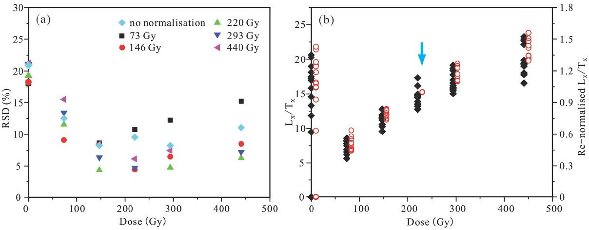
Fig 3
Comparison of the re-normalisation results with OSL signals of the re-normalisation dose of (a) 88 Gy, (b) 147 Gy and (c) 220 Gy.
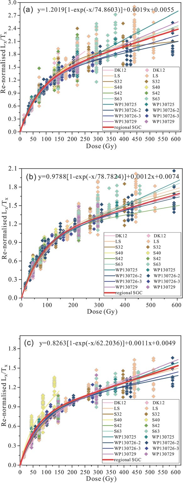
For all samples in the study area, the comparison made with re-normalisation using re-normalisation doses of 88 Gy, 147 Gy and 220 Gy (Fig. 3) shows that re-normalisation of sensitivity-corrected OSL signals of aliquots with a re-normalisation dose of 147 Gy yielded the smallest dispersion of the re-normalised OSL signals, which corresponds to a regenerative dose up to 250 Gy (Fig. 3b). As the characteristic saturation dose (D0) of quartz in most samples in this area is ~75 Gy, the comparison made in this study therefore shows that when using the Re-SGC method in quartz, re-normalisation of the sensitivity-corrected OSL signals (Lx/Tx) using an extra re-normalisation dose close to two times of the characteristic saturation dose (2D0) enables a value of De to be easily obtained, which has a smaller RSD of the re-normalisation OSL signals within the wide range of 0–200 Gy.
The SGC of a single profile
In this study, the SGC is established for each profile using the SAR-SGC, Re-SGC and LS-SGC methods. The results for representative profile LS and the other profiles are illustrated in Fig. 4 and supplementary Figs. S6–S14, respectively.
Fig 4
Comparison of re-normalised OSL signals (b, c and d) with the sensitivity-corrected OSL signals (a) from samples from the LS profile. Illustration of the potential SGCs established using (b) SAR-SGC, (c) Re-SGC and (d) LS-SGC methods. The diamonds represent the OSL signals of different samples, and the red curve represents the fitted SGC. In (b), the potential SGCs of different profiles are shown using the same colour as in the legend in Fig. 4-4b.
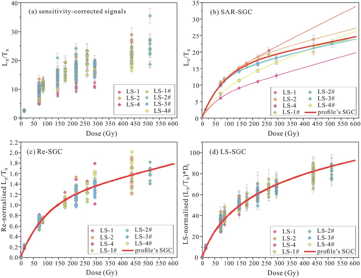
It is evident that the response of the sensitivity-corrected OSL signals (Lx/Tx) to the regenerative dose for samples from the profile is dispersed (Fig. 4a). Moreover, using the SAR-SGC method, the DRC would only be established for sensitivity-corrected OSL signals (Lx/Tx) of aliquots in a single sample after elimination of aliquots with substantial deviations. However, within the same profile, the DRCs established for different samples deviate substantially from each other (Fig. 4b), and it is difficult to determine a common growth curve that is suitable for samples from the same profile, with an acceptable degree of accuracy, using the SAR-SGC method.
Relative to the sensitivity-corrected OSL signal (Fig. 4a), based on the Re-SGC method, all of the sensitivity-corrected OSL signals (Lx/Tx) were re-normalised by dividing the OSL response (L147/T147) of the extra re-normalisation dose by 147 Gy, which is close to the 2D0 value. Therefore, the deviation of the re-normalised OSL signals among aliquots is reduced and a common SGC can be more reasonably established, especially within the dose range of 200 Gy, although the re-normalised signals are dispersed when De > 200 Gy (Fig. 4c).
When the LS-SGC method is used, the variation in the test-dose-corrected OSL signals (Lx/Tx*Dt) with the regenerative dose was fitted using a flexible function, and therefore, almost the same calibration level was reached among the regenerative doses for aliquots within the entire dose range. This does not alter the shape of the DRC of each aliquot, and it only minimises the difference between the DRCs of each aliquot. Almost the same dispersion range was obtained up to 300 Gy, and even up to 500 Gy, and therefore, a common DRC could be obtained for the samples from this profile (the red line in Fig. 4d).
In summary, a comparison based on samples from the same profile indicates the following. 1) The difference between sensitivity-corrected signals among samples was not substantially reduced using the SAR-SGC method, and therefore, it is difficult to establish a suitable SGC for the samples from a profile. 2) Using the Re-SGC method, differences in the sensitivity-corrected OSL signals among samples and aliquots can be effectively reduced when they are re-normalised with the OSL signal response to the extra re-normalisation dose, which is close to double the characteristic saturation dose (2D0). Therefore, an SGC suitable for samples from the same profile can be established with maximum De values up to 200 Gy. 3) Using the LS-SGC method, without considering any additional re-normalisation dose, the differences in the sensitivity-corrected signals among samples and aliquots from the same profile were uniformly reduced with a regenerative dose up to 300–500 Gy. Therefore, it is possible to establish an SGC suitable for samples from the entire area within a wide dose range using either the Re-SGC or LS-SGC method.
Regional SGC for the Jilantai area
By using the Re-SGC and LS-SGC methods, the difference in the re-normalised OSL signals among samples and aliquots can be effectively reduced, and therefore, we tried to establish a potential SGC that is suitable for the quartz fraction of sediments from the entire Jilantai region (hereafter termed the regional SGC). Based on the OSL signals of the quartz fraction in samples from different profiles within the entire Jilantai Basin, the regional SGCs were established with the fitting results illustrated in Fig. 5 (red lines). The function of the regional SGC obtained using the Re-SGC method is given below:
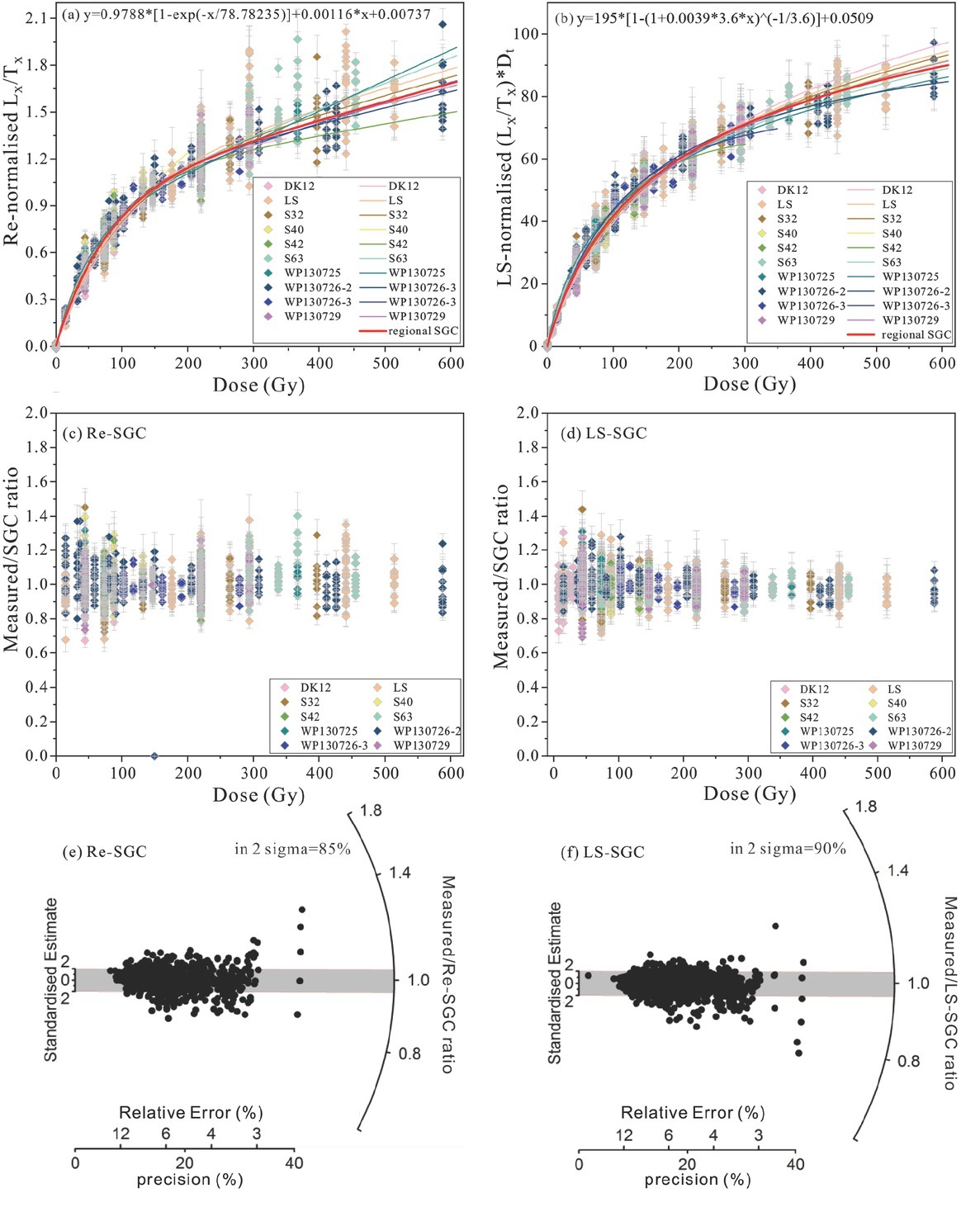
Fig 5
(a) The regional SGC (red curve) and DRCs from samples of profiles (the other coloured curves) established using the Re-SGC method. (b) The regional SGC (red curve) and DRCs of profiles (the other coloured curves) established using the LS-SGC method. (c) Ratios between the re-normalised data and the Re-SGC in (a), plotted against regenerative dose. (d) Ratios between the LS-normalised data and the LS-SGC in (b), plotted against regenerative dose. (e) Radial plot of the ratios shown in (c). (f) Radial plot of the ratios shown in (d). In the plots (e) and (f), the relatively high precision of 5–6 points, which scatter from the rest of the data points, was caused by OSL signal saturation.
and the function of the regional SGC obtained by the LS-SGC method using the GOK function is as follows:
In order to assess the quality of the SGCs, we calculated the ratios between the re-normalised Lx/Tx data (or LS-normalised Lx/Tx data) and the corresponding value on the SGC at the same dose and plotted them as a function of dose in Fig. 5c and d. Similarly, we plotted the ratios of De measured through normalised Lx/Tx data and that obtained from the SGC in a radial plot in Fig. 5e and f. There is no systematic dose dependency of the ratios for these two SGC methods, which is consistent with the observations on K-feldspar SGC (Li et al., 2018). In the radial plots in Fig. 5e and f, 85% and 90% of the total have ratios close to unity within 2σ range for the Re-SGC and LS-SGC methods, respectively, which closely matches statistical expectations (95%). These results imply the existence of a common regional SGC that can be established for the Jilantai area using the Re-SGC and LS-SGC methods.
Comparison of the re-normalised OSL signals, the fitting curves of samples from different profiles and the regional SGC (Fig. 5a and b) indicates the following. (1) Within the dose range of 0–200 Gy, the deviation in the shape of the fitting curves of samples from different profiles is less dispersed; therefore, a regional SGC can be established using either the Re-SGC or LS-SGC method. (2) Using the Re-SGC method, the regional SGC established from samples from different profiles shows deviations from the SGCs obtained from different profiles for regenerative doses > 200 Gy, which may be due to scattered re-normalised signals. (3) Relative to the re-normalised OSL signals obtained using the Re-SGC method, the re-normalised OSL signals obtained by the LS-SGC method are substantially less dispersed, and the regional SGC established from the LS-SGC method is almost overlapped by up to 300 Gy with DRCs obtained from most of the samples from a single profile. Deviations only occur when the regenerative dose is >300 Gy.
. Discussion
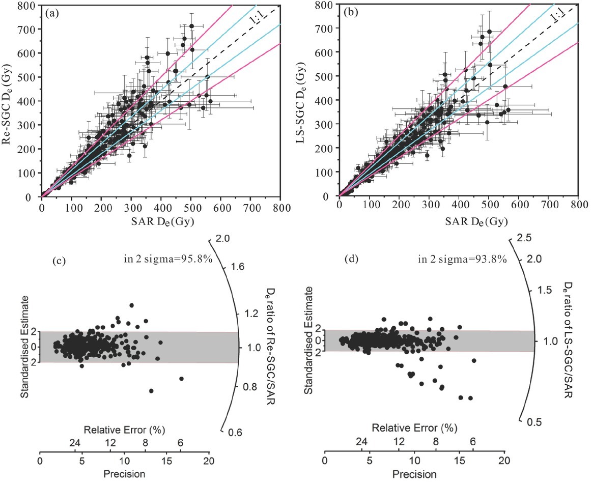
To validate the De values obtained through the regional SGC based on the Re-SGC and LS-SGC methods, a comparison was made with the De values obtained using the SAR protocol. For samples for which OSL signals were involved in establishing the SGC, we calculated the De values of 379 aliquots from the regional SGCs established using the Re-SGC and LS-SGC methods and made a comparison with the De values obtained using the SAR protocol. From the plots of De values obtained from the regional SGC using the Re-SGC method versus those obtained using the SAR protocol (Fig. 6a), it was found that 78% of the De values obtained from these two methods are consistent within a 20% error range of unity, and 53% were consistent within a 10% error range of unity. If the comparison is constrained within the range of De < 200 Gy, within which most of the De values are unsaturated, then 86% of the De values are consistent within a 20% error range of unity, and 63% are consistent within a 10% error range of unity. In a comparison of De values obtained from the regional SGC established using the LS-SGC method with those obtained from the SAR protocol (Fig. 6b), 56% of the De values are consistent within a 10% error range of unity and 81% are consistent within a 20% error range of unity. If the comparison is constrained within the range of De < 200 Gy, 84% of the De values are consistent within a 20% error range of unity, and 61% are consistent within a 10% error range of the unity. For De > 300 Gy, most of the data are scattered except for a small percentage which are distributed along the 1:1 line which is defined by the ratio of the De values obtained using the Re-SGC (or LS-RGC) method with those obtained from the SAR protocol. This indicates a large discrepancy in De values > 300 Gy between those obtained by using the regional SGCs established either using either the Re-SGC or LS-SGC method and those obtained using the SAR protocol (Fig. 6). This phenomenon may be the result of the saturation of the OSL signals. We also calculated the ratio of De values between those obtained from the SGCs and from the SAR protocol (Fig. 6c and d). From the De value ratios of Re-SGC to SAR, 95.8% of aliquots have ratios close to unity within the 2σ range (Fig. 6c). For the ratios of LS-SGC to SAR De values, 93.8% of ratios are close to unity within 2σ (Fig. 6d).
Fig 6
Comparison of De values obtained using the SAR protocol with those obtained using the Re-SGC (a) and LS-SGC (b) methods. The dashed black line is the 1:1 line, the solid blue lines define the 10% error range, and the solid pink lines define the 20% error range. (c) Radial plot showing ratios of the Re-SGC De values to the SAR De. (d) Radial plot showing the ratios of the LS-SGC De values to the SAR De. In the plot (d), 10 points with very low ratio were caused by OSL signal saturation.
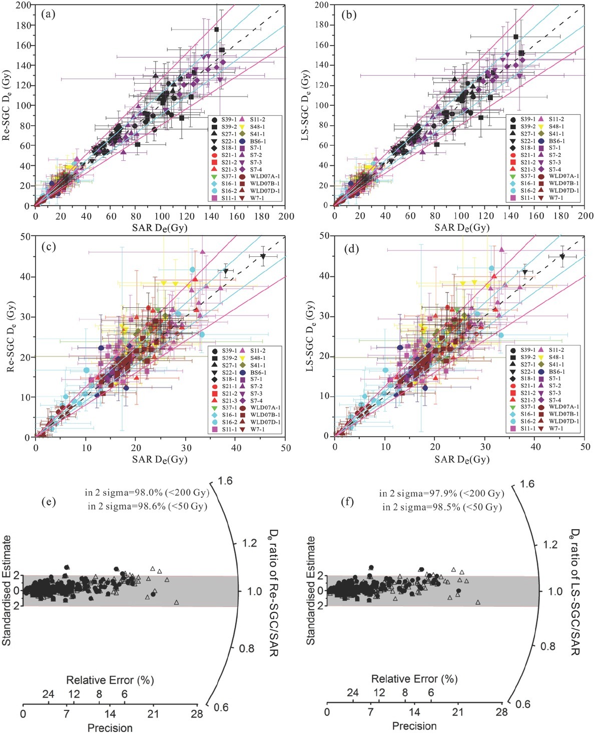
In order to further investigate whether the regional SGCs established using the Re-SGC and LS-SGC methods are widely applicable to samples from the study area, an additional comparison of De values (<200 Gy) was made on samples which were not involved in the establishment of the regional SGC. A total of 310 aliquots were used in the comparison. In general, the De values obtained using the regional SGC were consistent with those obtained using the SAR protocol within a 20% error range of unity (Fig. 7a and b). This situation is almost the same as that for the samples involved in the establishment of the regional SGCs (Fig. 6), which indicates that the two regional SGCs established from the limited sample set are also suitable for other samples from the Jilantai Basin. In detail, within the De range of 50–200 Gy, from the regional SGC established using the Re-SGC method, 69% of the aliquots yielded De values consistent with those obtained using the SAR protocol within a 10% error range of the unity, and 92% were consistent within the 20% error range of unity (Fig. 7a). From the regional SGC established using the LS-SGC method, 72% of the aliquots yielded De values consistent with those obtained using the SAR protocol within a 10% error range of unity, and 92% were consistent within the 20% error range of unity (Fig. 7b). However, for De <50 Gy, the number of aliquots with De values obtained using different methods consistent with those obtained using the SAR protocol within the 10% and 20% error ranges of unity was reduced significantly (Fig. 7c and d). In addition, the Re-SGC (or LS-SGC) and SAR De values are consistent, with more than 98% of the aliquots having ratios of SGC to SAR De clustered tightly within the 2σ range of unity (Fig. 7e and f).
Fig 7
Comparison of De values obtained using the SAR protocol with those obtained using the regional SGCs established using the Re-SGC (a and c) and LS-SGC (b and d) methods, for samples which were not used in the establishment of the regional SGCs. In these plots, the black dashed lines are the 1:1 ratio, and the areas enclosed by the blue solid lines are the 10% error range of unity, and the areas enclosed by the pink solid lines are the 20% error range of unity. (e) Radial plot showing the ratios of the Re-SGC De values to the SAR De. (f) Radial plot showing the ratios of the LS-SGC De values to the SAR De. Within (e) and (f), the data within 200 Gy are shown as open triangles and those <50 Gy as filled circles.
In summary, irrespective of which regional SGC is established, within the 10% error range, more than 50% of aliquots have De values consistent with those obtained using the SAR protocol, and within the 20% error range, more than 80% of aliquots have De values consistent with those using the SAR protocol. Similarly, more than 95% of the aliquots had ratios of SGC to SAR De consistent with unity at 2σ. Within the range of De < 200 Gy, the comparison of the De values obtained using regional SGCs established using the Re-SGC and LS-SGC methods with those obtained using the SAR protocol indicates that the De values obtained using these two regional SGCs are consistent. Therefore, a valid SGC can be produced for the Jilantai area within the 200 Gy range.
. Conclusions
Based on the OSL signals of small-aliquot quartz fractions of samples collected from different sedimentary environments in the Jilantai Basin, we have tried to establish a common SGC that is generally appropriate for samples from the area. Our main findings are as follows:
The inter-aliquot difference in sensitivity-corrected OSL signals can be effectively reduced using the Re-SGC and LS-SGC methods, and therefore, it is possible to establish a common SGC using these methods. However, the SAR-SGC method is not suitable for establishing a common SGC of quartz fractions, which is suitable for different samples from a profile or a region.
Using the Re-SGC method, selecting a re-normalisation dose that is close to double the characteristic saturation dose, 2D0, can reduce the variation in the shape of the DRCs among samples within a larger dose range. This is supported by a comparison in the RSD and dispersion of the renormalised OSL signals with different sizes of re-normalisation dose.
For De < 200 Gy, De obtained using the Re-SGC and LS-SGC methods is generally consistent with that obtained using the SAR protocol, which indicates that there is a common regional SGC in the Jilantai area. For the Jilantai area, the function of the regional SGC obtained by the Re-SGC method is y = 0.9788[1– exp(–x/78.78235)] + 0.00116x + 0.00737 , and the function of the regional SGC obtained by the LS-SGC method is y = 195[1– (1 + 0.0039 × 3.6 × x)^(–1/3.6)] + 0.0509.