1. INTRODUCTION

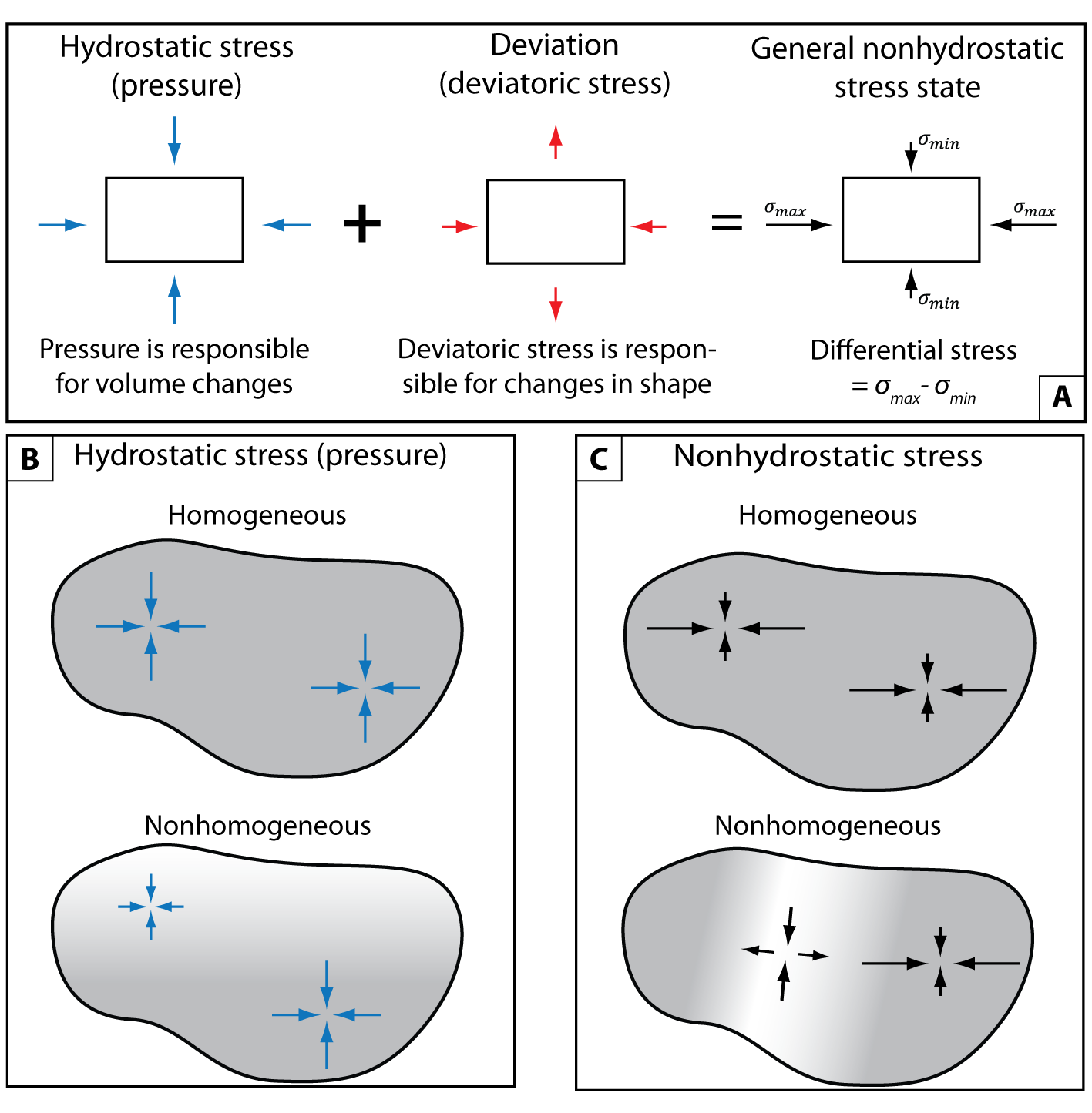
Our understanding of geological processes requires that we can accurately model how minerals, rocks and fluids behave chemically and mechanically in a wide range of pressure, temperature and stress conditions. Commonly, such conditions are characterized by increased pressure and temperature (P-T) compared to the Earth’s surface, thus making the direct observation problematic for processes like mineral deformation, fluid-mineral interaction and phase transformations in general. For example, the understanding of geodynamic processes such as plate subduction and mountain building largely relies on indirect observations such as the investigation of rocks that have recrystallized in subduction zones and are now found at the Earth’s surface. The preserved (quenched) mineral assemblages in metamorphic rocks are frequently interpreted in the framework of equilibrium thermodynamics, based on the experimentally produced mineral assemblages at laboratory conditions (e.g., Bucher & Frey, 2002; Spear, 1993). This approach has given us important insights on the range of conditions that are experienced by igneous and metamorphic rocks in natural environments. However, a major assumption of experimental petrology is that the stress state is hydrostatic and spatially homogeneous (e.g., fig. 1A, B), i.e., all the normal stresses in coexisting minerals and fluids are equal. It is important to note that by “hydrostatic stress state” we refer to the isotropy of the stress tensor (fig. 1A) and we do not imply that the stress can be calculated using the lithostatic stress gradient.

Figure 1.(A) Schematic illustration of the decomposition of a general, nonhydrostatic stress state into a mean-stress (hydrostatic part) and a deviation (deviatoric stress). In an elastically isotropic material, the hydrostatic and the deviatoric part of the stress control the changes in volume and shape, respectively. The differential stress ($\sigma_{\max} - \sigma_{\min}$) describes the difference between the largest and smallest normal stresses and it is proportional to the deviation from hydrostatic conditions. (B) Under hydrostatic stress, all the normal stresses acting on a point are equal to each other. If the stress state is the same at every point in a system, the stress is said to be homogenous. If the magnitude of the hydrostatic stress varies across the system, the hydrostatic stress is nonhomogeneous. (C) Under a nonhydrostatic stress state, the normal stress components acting on a point are not equal one another. If the nonhydrostatic stress is the same at every point in the system, the system is under a homogeneous, nonhydrostatic stress. In a system under a non-homogenous, nonhydrostatic stress, the normal components can vary in magnitude, sign and orientation across the system.

An interesting realization is that all Gibbs-energy minimization algorithms and mineral equilibrium software (e.g., Connolly, 2005, 2017; de Capitani & Petrakakis, 2010; Riel et al., 2022) rely on this hydrostatic approximation. This means that in these algorithms the pressure of each phase is the same (i.e., it is homogeneous) and the stress tensor is assumed to be isotropic independently of the nature of the material and the loading configuration (fig. 1B). In mechanically weak mineral assemblages, the hydrostatic approximation seems to provide an adequate description of the state of stress in the Earth, because all of the normal stress components will be almost equal to each other (e.g., Moulas et al., 2019). However, because of its rheological properties, the Earth’s lithosphere can sustain significant levels of nonhydrostatic stress with macroscopic differential stresses that may reach up to 0.5–1 GPa (Brace & Kohlstedt, 1980; Prieto et al., 2012). In this work, we use the term nonhydrostatic stress to refer to the general state of stress where the stress tensor is not isotropic. For isotropic materials it is common to refer to the isotropic part of the stress tensor as hydrostatic stress (i.e., the pressure, when adjusted for sign conventions), whereas the anisotropic part is referred to as the deviatoric stress (fig. 1A). In principle, for elastically isotropic materials, the pressure is solely related to volume changes while the deviatoric stress induces only shape changes. However, for a general anisotropic material (i.e., for any crystal with crystallographic symmetry lower than cubic) even a purely hydrostatic state of stress will not result in a purely isotropic strain state. Therefore, in solid minerals, volume changes are generally influenced also by the deviatoric part of the stress. In this case, the decomposition of the stress tensor into a hydrostatic and deviatoric part does not hold a precise physical meaning (Augusti et al., 1969). To avoid confusion, in this work we use the term “nonhydrostatic stress” to describe a general state of stress in which the stress loading is not equal from every side of the crystal. By differential stress we refer to the difference between the maximum and the minimum normal components (eigenvalues) of the stress tensor, which scales proportionally to the degree of anisotropy of the stress tensor (fig. 1A).

In presence of fast tectonic deformations, the differential stress in the Earth’s lithosphere can reach several hundreds of MPa in magnitude (e.g., Andersen et al., 2008). Nonhydrostatic stresses can also be observed when relatively strong viscous creep flow laws are employed in the modeling of subduction settings (e.g., Reuber et al., 2016). At the mineral scale, nonhydrostatic stress states with differential stress up to 1 GPa are observed when strong mineral hosts enclose minerals with different elastic properties (Campomenosi et al., 2018; Gonzalez et al., 2021; Kohn et al., 2023; Moulas et al., 2020, 2023). In general, any change in the pressure and temperature experienced by a solid mineral aggregate will generate stresses at the grain-scale level simply because different minerals respond differently to the applied stress/strain conditions. In recent years, an increased number of studies have highlighted the importance of volume changes during mineral reactions and phase transitions (Gillet et al., 1984; Van der Molen & Van Roermund, 1986; Zheng et al., 2018).

These effects become particularly significant in a confined environment such as the one expected in the deep Earth. In such cases, mechanical models predict the development of GPa-level stress and pressure differences between the host mineral and the inclusion (Plümper et al., 2022; Zhukov & Korsakov, 2015). Moreover, in multiphase systems with coexisting minerals and fluids, pressure and stress gradients are intrinsically generated due to changes in the contact area of the solid grains (e.g., Dahlen, 1992; Gallagher et al., 1974; Pollard & Fletcher, 2005, p. 194). However, despite the quantification of the interplay between stress, thermodynamic equilibria and reactions being essential for understanding many key geological processes, the magnitude of the effect of nonhydrostatic stresses on fluid-mineral and mineral-mineral equilibria is still actively debated.

Gibbs (1876) first realized that the classic expression of free energy and phase equilibria was only applicable to hydrostatic condition and discussed the influence of a nonhydrostatic stress on the equilibrium between a solid and a fluid of the same composition. However, the magnitude of the effect of nonhydrostatic stresses on fluid-mineral and mineral-mineral equilibria is still actively debated among researchers who, sometimes, have incompatible views about the use of various thermodynamic formulations (e.g., Hess & Ague, 2021; Hobbs & Ord, 2015; Tajčmanová et al., 2015; Wheeler, 2014). Several experiments have tried to shed light on such controversies by imposing nonhydrostatic stress on pure substances that experience phase transitions (Hirth & Tullis, 1994; Hobbs, 1968; Richter et al., 2016; Vaughan et al., 1984; Zhou et al., 2005). However, recent studies that combine data from experiments and models of rock deformation suggest that the stress field in such experiments is nonhomogeneous, and therefore the experimental results are not diagnostic (Cionoiu et al., 2019, 2022; Ji & Wang, 2011; Moulas et al., 2013). The development of pressure gradients in these experiments is directly proportional to the applied far-field differential stress (Cionoiu et al., 2022). Thus, in mechanical experiments, it is difficult to resolve whether the observed phase transitions are controlled by the nonhydrostatic stress state (which in this work we call the direct effect of nonhydrostatic stress) or if they are caused by local pressure concentrations due the presence of a nonhomogeneous stress within the sample (i.e., the indirect effect of nonhydrostatic stress, fig. 1C). Apart from the problem of nonhomogeneous stress distribution, typical rock-deformation experiments do not allow us to resolve the stress state within the sample during the occurrence of phase transitions and mineral reactions. The products of such experiments are typically studied after the sample has been recovered and the only available information about its evolving stress state is related to the far-field loading conditions. Therefore, the actual phase distribution at the end of the experiment may not correspond to an instantaneous equilibrium phase distribution but may be influenced by the entire stress/strain history of the sample (e.g., Cionoiu et al., 2022). For this reason, without knowledge of the stress distribution within the sample, it is extremely difficult to assess the direct effect of stress on mineral equilibria.

The presence of nonhydrostatic stress conditions and stress gradients is not just limited to solid aggregates, but they can also be developed in porous system where solid grains are in contact and react with fluid phases, such as aqueous fluids and melts (Gallagher et al., 1974). Fluid flow and associated hydration and dehydration reactions play a fundamental role in many phenomena in the lithosphere, such as the dynamics of shear zones (e.g., Austrheim, 1987), the generation of earthquakes (e.g., Brantut et al., 2017; Ferrand et al., 2017), or rheological weakening of rocks (e.g., Jolivet et al., 2005; Kaatz et al., 2021; Moulas et al., 2022). In magmatic systems, the production of melt due to phase transitions can have a dramatic influence on the rheological properties of porous rocks and on the overall magma dynamics (e.g., Hirth & Kohlstedt, 1995; Schmeling et al., 2012; Yarushina & Podladchikov, 2015). The accurate prediction of fluid-solid reactions is also central in industrial processes with examples that range from the prediction of mineral reactions in geological carbon sequestration (e.g., Kelemen & Hirth, 2012), to the assessment of the volume changes during geothermal energy extraction (Erfani et al., 2019) and to the engineering of underground long-term nuclear waste repositories (Spycher et al., 2003).

While in hydrostatic thermodynamics the Gibbs potential can be adopted to find equilibrium assemblages, there is no experimentally verified, thermodynamic theory for nonhydrostatic reactions in deforming geomaterials. To assess which thermodynamic description is the most appropriate in describing mineral phase equilibria under nonhydrostatic stresses, we performed atomistic computer simulations with molecular-dynamics (MD). With this approach, we can evaluate the evolution of the trajectories of the individual atoms that constitute a two-phase solid-fluid system, under prescribed stress and temperature conditions. With MD simulations, the direct influence of several controlled nonhydrostatic stress states on the mineral-fluid equilibrium can be assessed independent of any assumption regarding the thermodynamic potential of the system. Moreover, in MD simulations the stress in the solid phase can be kept homogeneous, allowing us to isolate the direct effect of the nonhydrostatic stress on the perturbation of the equilibrium, avoiding the development of local stress concentrations which, as deduced by experiments, may indirectly affect the equilibrium. For our MD simulations we adopted the Lennard-Jones (LJ) method (Lennard-Jones, 1924a, 1924b), which provides a numerical representation of an idealized network of atoms and the interatomic potential that controls the dynamics of the individual atoms. This allowed us to explore the equilibrium states of a coexisting solid and fluid in an idealized one-component system under controlled stress conditions.

We begin our paper by introducing the problem of stress gradients in fluid-mineral systems and then proceed with a short summary of the previous thermodynamic analysis related to the single-component solid-fluid equilibration. We then introduce our MD models in relation to the problem of solid-fluid equilibration under stress. Our approach follows similar studies from the literature but considers the effects of nonhydrostatic stress under confined conditions (i.e., initial pressure larger than zero). Our simulations show that, at constant temperature, a positive change of the fluid equilibrium pressure is always to be expected, whether the applied nonhydrostatic stress is compressive or tensile. For small applied differential stresses, the change in fluid pressure ($P^{f})$ required to maintain the solid-fluid equilibrium at constant temperature is small and approximately one order of magnitude less than the differential stress generated in the solid. On the other hand, our results show that, for the particular loading configuration, the mean stress of the solid ($\overline{\sigma^{s}})$ changes considerably in response to the nonhydrostatic stress applied to it. Therefore, when the solid is under differential stress, its $\overline{\sigma^{s}}$ deviates from the $P^{f}$ with which it is in equilibrium, leading to a decoupling between the “pressure” (i.e., $- \overline{\sigma^{s}}$) of the solid phase and the pressure of the solid-fluid thermodynamic equilibrium. With this approach, we can therefore assess the magnitude of the deviation of phase equilibria from the hydrostatic approximation in simple systems under nonhydrostatic stress. Finally, we discuss the magnitude of the stress inhomogeneities that arise in solid-fluid multiphase systems and which stress measure should be taken as a proxy of the thermodynamic pressure in order to accurately describe reactions.

2. STRESS IN FLUID-SOLID MULTIPHASE SYSTEMS

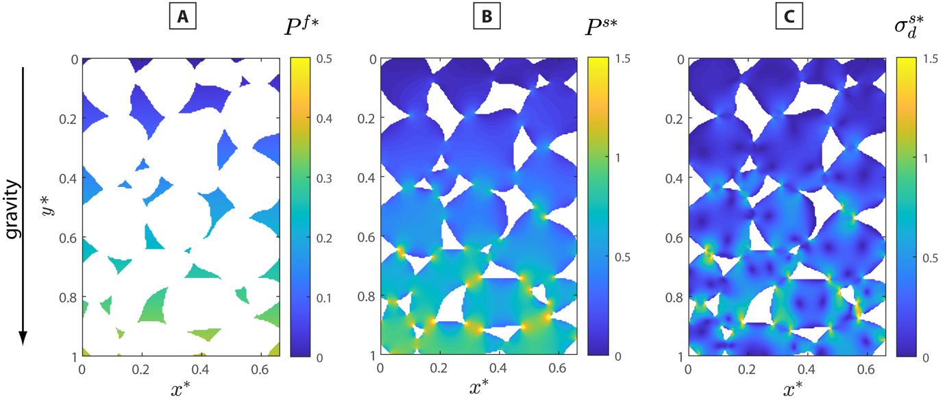
Many processes in the Earth are intrinsically related to the evolution of multiphase systems in which solid mineral phases are coupled with fluid phases, such as aqueous fluids and melts. Theoretical considerations and experimental studies have verified that in porous and granular rocks stresses are not distributed homogeneously (Gallagher et al., 1974). In particular, a granular rock having a fluid-filled porosity is expected to develop stress gradients because of the inability of the fluid to sustain large deviatoric stresses. Even without far-field tectonic loads, stress gradients are developed due to the presence of gravity and the occurrence of stress concentration along grain contacts. We refer to such conditions as quasi-static since true lithostatic conditions require, inter alia, that the rock is stratified with respect to its density (e.g., Moulas et al., 2019). Porous rocks with lateral density gradients do not satisfy this condition but, in the absence of far-field stresses can be approximated as static, at least macroscopically. In order to calculate and show the mean-stress (pressure) gradients developed in a granular rock under the influence of gravity we consider a schematic two-dimensional section of a model rock as it was provided in the work of Dahlen (1992, his fig. 1). In addition, we adopt a viscous mechanical model with a gravity field (the details of the calculation are reported in appendix A). Figure 2A shows that when the porosity is interconnected, the fluid will always experience a hydrostatic stress gradient. On the contrary, the solid grains will experience different levels of stress due to the changes in the contact area between each grain (e.g., Pollard & Fletcher, 2005, p. 194). As a consequence, in rocks that are porous or have a granular structure, local stress gradients are always developed, even if their macroscopic pressure gradient is “lithostatic” (fig. 2B, C). The presence of stress and pressure gradients may have important implications on our interpretations of processes in the Earth.

Figure 2.Mechanical stress state of a porous system composed of a solid porous matrix and a fluid (geometry after fig. 1 of Dahlen, 1992). All quantities are presented in dimensionless form (indicated by a star, see appendix A for details). Despite the system is assumed to be under its own weight and without any far-field stress (lithostatic), the solid-fluid coexistence led to the development of local nonhydrostatic stress in the solid matrix. (A) Pressure of the interconnected fluid ($P^{f*}$- colored region). (B) Negative mean stress (pressure) of the solid grains ($P^{s*}$ - colored region). (C) Differential stress of the solid matrix ($\sigma_{d}^{s*}$- colored region). The non-zero differential stress in the solid grains indicates that their state of stress is not hydrostatic.

Current numerical models that describe the mechanical and chemical evolution of such systems assume that the fluid pressure is equal to the rock pressure (e.g., Yang & Faccenda, 2020) and that the chemical reactions are controlled by the pressure of the fluid phase (e.g., Schmalholz et al., 2020). From a thermodynamic perspective, these assumptions imply that the solid matrix and the coexisting fluid are assumed to be under hydrostatic-stress conditions. Therefore, within this approximation, the resulting phase equilibria and reactions are described by the minimization of Gibbs free energy at constrained $P - T$ conditions. However, as we have shown, the presence of a nonhomogeneous-stress distribution at the grain scale breaks the fundamental assumptions behind the use of Gibbs potentials, i.e., a hydrostatic stress tensor and homogeneous stress field. The presence of nonhydrostatic stress can lead to changes of the physical conditions at which phase equilibria and reactions take place. These changes can have a large effect on the chemical and mechanical evolution of the system. For example, the production of fluid/melt during mineral reactions and phase transitions can have a dramatic influence on the rheological properties of porous rocks. This is because the effective bulk and shear viscosity of partially molten rocks are inversely dependent on porosity and melt fraction (e.g., Schmeling et al., 2012; Yarushina & Podladchikov, 2015). Such effects become even more relevant if we consider cases in which the fluid/melt flow is driven by pressure gradients in tectonically stressed, porous rocks (e.g., Connolly & Podladchikov, 2004; Spiegelman & McKenzie, 1987).

Therefore, the quantification of the effect of nonhydrostatic stress on mineral phase equilibria is crucial to describe the mechanical properties and the mineralogy of porous, multiphase, reactive rocks. However, such perturbations cannot be evaluated directly in natural systems since, as shown in figure 2, they do not provide simple example of homogeneous loading in the solid phase. This implies that, similarly to what observed in experiments, also in natural samples the displacements of thermodynamic equilibria due to the nonhydrostatic stress state (direct effect) cannot be separated from the effect due to stress concentrations and pressure gradients (indirect effect). Such perturbations cannot be evaluated either by existing numerical models which are purely mechanical, and therefore cannot account for the two-way feedback between the deformation and the nonhydrostatic thermodynamic response. Models that are able to assess the microscopic scale behavior of multiphase systems under homogeneous stress in the solid phase, such as those that can be performed with MD, are therefore required to assess the direct effect of a homogeneous, nonhydrostatic stress on the thermodynamic phase equilibria in deformed systems.

3. THERMODYNAMICS OF SOLID-FLUID EQUILIBRIUM AT NONHYDROSTATIC CONDITIONS

The thermodynamics of systems which have a nonhydrostatic stress state has been the topic of several recent studies (Hess & Ague, 2021; Hobbs & Ord, 2016; Tajčmanová et al., 2015; Wheeler, 2014). In those studies, different interpretations are proposed regarding the role of pressure (also called “thermodynamic pressure”). In this work, we will highlight the difference between the fluid and solid pressures in a thermodynamically equilibrated system. As it will become clear later, the fluid and solid pressures can both be considered “thermodynamic” as they can be derived from thermodynamic principles. The main difference is that the equilibrium fluid pressure is related to the solid-fluid coexistence conditions while the solid “pressure” ($- \overline{\sigma^{s}}$) is related to the volumetric response of the solid.

In systems under nonhydrostatic conditions that comprise solids in contact with fluids, chemical reactions can involve dissolution of solid phases in the fluid, chemical reactions in the fluid and subsequent precipitation of the newly reacted material on the stressed solid. The equilibrium between a solid under nonhydrostatic stress and fluids was first investigated by Gibbs (1876, pp. 34–520). Assuming that temperature is homogeneous in the system and that the deformations are small, Gibbs derived the equilibrium between a solid and a fluid in a single component system (his eq 386 and eq 3 in Sekerka & Cahn, 2004):

$$\frac{{\widehat{U}}^{s}}{{\widehat{\Omega}}_{0}^{s}} - \frac{T{\widehat{S}}^{s}}{{\widehat{\Omega}}_{0}^{s}} + \frac{P^{f}{\widehat{\Omega}}^{s}}{{\widehat{\Omega}}_{0}^{s}} = {\widehat{\mu}}^{f}{\widehat{\rho}}^{s} \tag{1}$$

where T (K) is the absolute temperature of the system at equilibrium. Superscript s refers to variables of the solid, where ${\widehat{\Omega}}_{0}^{s}$ (in m³) is the reference volume of the solid in the undeformed configuration, ${\widehat{U}}^{s}$ its energy (J), ${\widehat{S}}^{s}$ its entropy (J/K), and ${\widehat{\rho}}^{s} = \frac{m}{{\widehat{\Omega_{0}}}^{s}}$ (kg/m³) the mass density of the considered component in the solid at the reference state (notation is summarized in table 1). Superscript f refers to variables of the fluid, with $P^{f}$ (Pa) being the pressure of the fluid, and ${\widehat{\mu}}^{f}$ (J/kg) being the chemical potential of the substance of the solid in the fluid. By considering the atom density of the substance of the solid in the undeformed state $\rho_{a}^{s} = \frac{N}{{{\widehat{\Omega}}^{s}}_{0}}$ (m^-3) and expressing the per-atom chemical potential as $\mu^{f}$, we can divide equation (1) by $\rho_{a}^{s}$ to obtain:

$$u^{s} - Ts^{s} + P^{f}\omega^{s} = \mu^{f} \tag{2}$$

where $u^{s} = \frac{{\widehat{U}}^{s}}{{\widehat{\Omega}}_{0\ }^{s}\rho_{a}^{s}\ }$, $s^{s} = \frac{{\widehat{S}}^{s}}{{\widehat{\Omega}}_{0\ }^{s}\rho_{a}^{s}\ }$, $\omega^{s} = \frac{{\widehat{\Omega}}^{s}}{{\widehat{\Omega}}_{0\ }^{s}\rho_{a}^{s}\ }$, $\mu^{f} = \frac{{{\widehat{\mu}}^{f}\widehat{\rho}}^{s}}{\rho_{a}^{s}}$ are now per-atom quantities.

Starting from the work of Gibbs (1876), Frolov and Mishin (2010) have explored in more detail the case of a single component solid in equilibrium with its liquid (i.e., a single-component fluid with the same composition of the solid). Their analysis has extended the theory to include also the anisotropic elastic properties of the solid phase, which is particularly relevant for minerals that are elastically anisotropic (e.g., Nye, 1985). Here we follow Sekerka and Cahn (2004) and Frolov and Mishin (2010) and develop a relationship that describes the effect of nonhydrostatic stresses on the solid-fluid equilibrium in single-component systems. We start by recognizing the expression of the Helmholtz free energy of the solid, $\psi^{s}$, in equation (2):

$$\psi^{s} = \ u^{s} - Ts^{s} \tag{3}$$

Therefore, using the previous equation, equation (2) can be written as:

$$\psi^{s} + P^{f}\ \omega^{s} = \mu^{f} \tag{4}$$

When both the solid and the fluid are under a homogeneous and hydrostatic stress, the pressure of the fluid $P^{f}$is equal to the pressure of the system $P_{H}$. In that case, the Gibbs free energy (per atom) of the solid is:

$$g_{H}^{s} = \ \psi_{H}^{s} + P_{H}\omega_{H}^{s} \tag{5}$$

where the subscript H refers to the properties in the system where both the solid and the fluid are under the same hydrostatic conditions. By rearranging equation (4) and substituting the result in equation (5), we arrive to the usual equilibrium condition for a single component solid in contact with its pure melt under hydrostatic stress:

$$g_{H}^{s} = \mu_{H}^{f} \tag{6}$$

When the solid is taken from the hydrostatic state to nonhydrostatic conditions its energy changes, and therefore, in order to preserve the equilibrium, the chemical potential of the component of the solid in the fluid must change accordingly. The variation of the Helmholtz energy of the solid with stress/strain can be evaluated by expressing its differential with respect to the applied strain and the temperature:

$${d\psi}^{s} = \omega_{H}^{s}\sum_{i,j = 1,2,3}^{}{\sigma_{ij}^{s}d\varepsilon_{ij}^{s}} - s^{s}dT \tag{7}$$

where $\omega_{H}^{s}$ is the volume per atom of the solid in the hydrostatic reference state used to define the strain, and $\sigma_{ij}^{s}$ and $\varepsilon_{ij}^{s}$ are the Cauchy stress tensor and the small strain (i.e., Lagrangian infinitesimal) tensor of the solid, respectively. Following the usual convention in continuum mechanics, $\sigma_{ij}^{s}$ and $\varepsilon_{ij}^{s}$ are positive in tension. Equation (7) shows that, for the single component solid, when the system is kept at constant temperature, the variation of the Helmholtz free energy is only due to the applied strain. Therefore, for an isothermal process, the Helmholtz free energy of the solid is equal to the elastic energy, and any change in the strain state of the solid will increase its free energy. This increase in the specific (per atom) elastic energy occurs whether the strain in the solid is tensile or compressive.

Assuming that the solid is linear elastic and that the applied strain is small, Hooke’s law can be used to express the linear relationship between the Cauchy stress and the applied strain: $\sigma_{ij} = \ C_{ijkl}\varepsilon_{kl}$, with $C_{ijkl}$ the 4^th-rank elastic stiffness tensor of the solid (with components in pressure units, Pa). Under this assumption, the specific Helmholtz free energy of the solid can be found by integrating equation (7) for small variations in strain (assuming constant temperature):

$$\begin{align} \psi^{s} &= \frac{\omega_{H}^{s}}{2}\sum_{i,j = 1,2,3}^{}{\sigma_{ij}^{s}\varepsilon_{ij}^{s}} \\ &= \frac{\omega_{H}^{s}}{2}\sum_{i,j,k,l = 1,2,3}^{}{C_{ijkl}^{s}\varepsilon_{ij}^{s}\varepsilon_{kl}^{s}} \\ &= \ \frac{\omega_{H}^{s}}{2}\sum_{i,j,k,l = 1,2,3}^{}{D_{ijkl}^{s}\sigma_{ij}^{s}\sigma_{kl}^{s}} \end{align} \tag{8}$$

where $D_{ijkl}^{s} = \ {C^{s}}_{ijkl}^{- 1}$ is the elastic compliance tensor of the solid. At constant temperature, a solid can increase its energy by increasing its elastic stress, and therefore the Helmholtz energy (eq 8) of the linear-elastic solid is an implicit function of its elastic stress state (not necessarily hydrostatic) and of the absolute temperature, independent from the mechanism that has generated the stress. In other words, given a specific temperature and stress state, the specific Helmholtz energy of the solid is the same whether the solid is in contact with a fluid or with another solid.

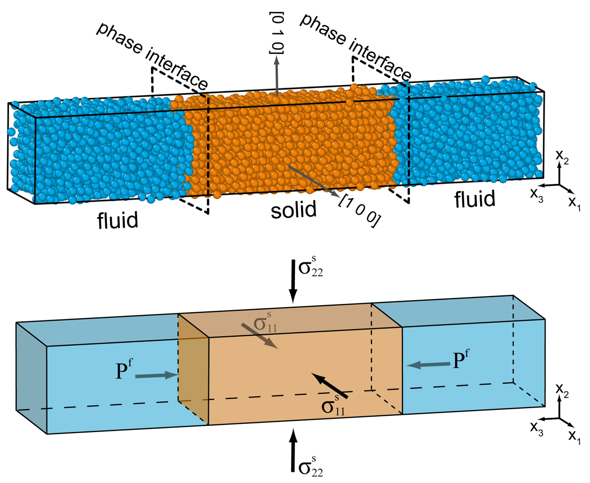
Since we are interested in describing the equilibrium between a solid and a fluid, we can exploit the requirements of mechanical equilibrium, which imposes that the normal stress of the solid orthogonal to the solid-fluid interface is equal in magnitude and opposite in sign to the pressure of the fluid. For example, we can consider a configuration in which a rectangular block of the solid is in contact with a fluid along two faces and is oriented so that the principal stress component $\sigma_{33},$ along the Cartesian $x_{3}$ direction, is orthogonal to the solid–fluid interface (e.g., fig. 3). In this case it follows that $\sigma_{33} = - P^{f}$. If we now assume that the shear stresses are zero, and the stress state is homogeneous in the solid, we can represent the specific Helmholtz energy of the solid as a function of this stress and the absolute temperature:

$$\begin{align} \psi^{s} &= \psi^{s}\ \left( T,\ - \sigma_{11},\ - \sigma_{22},\ - \sigma_{33}\ \right) \\ &= \psi^{s}\ \left( T,\ - \sigma_{11},\ - \sigma_{22},\ P^{f}\ \right) \end{align} \tag{9}$$

Figure 3.(A) Snapshot of the simulated coexisting LJ system equilibrated at hydrostatic conditions. Atoms belonging to the fcc solid and fluid layers are shown in orange and blue, respectively (see appendix C for details on the distinguishing procedure). Rendering performed with the OVITO software (Stukowski, 2010). The crystallographic directions [1 0 0] and [0 1 0] of the solid are aligned with the reference axes $x_{1}$ and $x_{2}$, respectively. (B) Stress configuration of the solid in the MD simulations. The strain applied to the solid is axially-symmetric $(\varepsilon_{11} = \varepsilon_{22}$) resulting (because of the crystallographic symmetry and orientation of the solid) in an axially-symmetric stress $\left( \sigma_{11}^{s} = \sigma_{22}^{s} \right)$. Because of mechanical equilibrium $\sigma_{33}^{s} = - P^{f}$. The shear stress components of the solid are zero.

We can now consider the equilibrium between a nonhydrostatically stressed solid and a fluid. Gibbs (1876) showed that the condition outlined above (i.e., eq 4) for the equilibrium between a single-component, homogeneous, hydrostatic solid and a fluid is formally valid even when the solid is loaded in a nonhydrostatic manner. However, the quantities that appear in the equation assume different values in the hydrostatic and the nonhydrostatic configuration, since they directly depend on the stress configuration. Assuming that the temperature $T$ is uniform in the system and that the geometrical configuration is as in figure 3, we can rewrite the equilibrium condition to highlight which quantities are functions of the stress state of the solid (eq 9 of Sekerka & Cahn, 2004):

$$\begin{align} \mu^{f}\ \left( T,\ P^{f} \right) &= \ u^{s}\left( T,\ - \sigma_{11},\ - \sigma_{22},\ P^{f} \right)\ \\ &\quad - T\ s^{s}\left( T,\ - \sigma_{11},\ - \sigma_{22},\ P^{f} \right) \\ &\quad + \ P^{f}\ \omega^{s}\left( T,\ - \sigma_{11},\ - \sigma_{22},\ P^{f} \right) \\ &= \ \psi^{s}\left( T,\ - \sigma_{11},\ - \sigma_{22},\ P^{f} \right) \\ &\quad + \ P^{f}\ \omega^{s}\left( T,\ - \sigma_{11},\ - \sigma_{22},\ P^{f} \right) \end{align} \tag{10}$$

where $T$ is the temperature of equilibrium between the fluid and the nonhydrostatic solid. Equation (10) highlights that the volume of the solid, and therefore its density, is controlled by its full stress state and not only by the pressure of the fluid to which it is in contact. It also shows that, in agreement to equation (8), the equilibrium between the solid and the fluid is determined by the complete stress state of the solid and not by the $P^{f}$ alone. For example, in a system at constant temperature, a nonhydrostatic stress applied to the solid will always increase its specific Helmholtz energy, whatever the strain/stress state (see eq 7). Therefore, one can already expect qualitatively from equation (10) that at constant temperature the chemical potential of the component of the solid in the fluid $\left( \mu^{f} \right)$ must vary in order to preserve the equilibrium between the stressed solid and the fluid. In a single-component system at constant $T$, the variation of $\mu^{f}$ can only be generated by a variation of the pressure $P^{f}$. The latter implies that the fluid must change its pressure in order to preserve the equilibrium with a stressed solid.

Frolov and Mishin (2010) have derived a full description that relates the changes in temperature of the system, pressure of the fluid, and nonhydrostatic stress of an elastically anisotropic solid for a solid-fluid system at equilibrium. Such a relationship can be obtained by starting from the expressions of the differentials of the internal energy of the solid and of the chemical potential of the fluid for a variation of stress state and entropy of the solid and of temperature and pressure of the fluid, respectively:

$$\begin{align} du^{s} &= T_{H}ds^{s} + \omega_{H}^{s}\sum_{i,j = 1,2,3}^{}{\ \sigma_{ij}^{s}\ d\varepsilon_{ij}^{s}} \\ {d\mu}^{f} &= \ - s_{H}^{f}dT + \omega_{H}^{f}dP^{f} \end{align} \tag{11}$$

where the subscript H refers to quantities evaluated in the hydrostatic state as before. The equation that describes the change in the equilibrium $P^{f}$ and temperature of the system for small departures from the hydrostatic state, is obtained by taking the full differential of equation (10) and substituting the relationships of equation (11). By linearizing the differentials of the resulting equation (first-order Taylor expansion), and assuming a linear elastic relationship between strain and stresses, Frolov and Mishin (2010) integrated the resulting equation from the initial hydrostatic state to an (nonhydrostatic) equilibrium state:

$$\begin{align} \Delta s_{H}\left( T - T_{H} \right) &+ \frac{1}{2}\left( \frac{\partial\Delta s}{\partial T} \right)_{H}\left( T - T_{H} \right)^{2} \\ &- \Delta\omega_{H}\left( P - P_{H} \right) \\ &\quad - \frac{1}{2}\left( \frac{\partial\Delta\omega}{\partial P} \right)_{H}\left( P - P_{H} \right)^{2} \\ &-\left( \frac{\partial\Delta\omega}{\partial T} \right)_{H}\left( T - T_{H} \right)\left( P - P_{H} \right) \\ &+ \frac{\omega_{H}^{s}}{2}\sum_{i,j,k,l = 1,2}^{}{D_{ijkl}^{s}q_{ij}^{s}q_{kl}^{s}} = 0 \end{align} \tag{12}$$

$\Delta s_{H} = \ s_{H}^{f} - s_{H}^{s}$ and $\Delta\omega_{H} = \ \omega_{H}^{f} - \omega_{H}^{s}$ are, respectively, the differences between the atomic entropy and volume of the fluid and the solid in the reference hydrostatic state. The tensor $q_{ij}^{s} = \ \sigma_{ij}^{s} + \delta_{ij}P^{f}$ expresses the deviation of the stress components of the solid from the $P^{f}$. We note that the tensor $q_{ij}^{s}$ does not represent the deviatoric stress tensor of the solid phase, since it relates the components of the stress tensor of the solid to the $P^{f}$, and not to the $\overline{\sigma^{s}}$. As it will be shown later, under nonhydrostatic stress the $\overline{\sigma^{s}}$ and the $P^{f}$ can assume different values even at equilibrium, leading to a deviation of the components $q_{ij}^{s}$ from those of the deviatoric stress tensor of the solid phase.

For our geometric configuration (fig. 3) and since the fluid cannot support shear stresses, the shear stress components in the $x_{1} - x_{2}$ plane are parallel to the solid-fluid interface implying that the components $\sigma_{13}^{s}$, $\sigma_{23}^{s}$, and their symmetric equivalents $\sigma_{31}^{s}$, $\sigma_{32}^{s}$, are zero. Moreover, as discussed above, mechanical equilibrium prescribes that one of the normal components of the stress of the solid must be numerically equal to the negative of the fluid pressure (in our case $\sigma_{33}^{s} = - P^{f}$, see fig. 3B). Such mechanical constraints limit the summation in equation (12) to $i,j,k,l\ = \ 1,2$, since all the components of the tensor $q_{mn}^{s}$ with indices m = 3 and/or n = 3 become zero. We note that, despite the simplification, this remains a completely general 3D problem because we do not impose any arbitrary restriction on the value of the stress components.

Equation (12) is obtained by assuming that the solid is anisotropic and linear elastic, the deformations are small (i.e., negligible volume changes) and the elastic properties of the solid are constant with stress and strain. Starting from equation (12), one can evaluate the effect of the stress state of the solid on the $T$ and the $P^{f}$ at equilibrium for any thermodynamic path. For example, at isobaric conditions (i.e., the pressure of the fluid is kept constant) and neglecting second order terms, equation (12) becomes:

$$T - T_{H} = \ - \ \frac{\omega_{H}^{s}}{2\ \Delta s_{H\ }}\sum_{i,j,k,l = 1,2}^{}{D_{ijkl}^{s}q_{ij}^{s}q_{kl}^{s}} \tag{13}$$

Equation (13) implies that the temperature of equilibrium changes from the initial hydrostatic state ($T_{H})$ to the new equilibrium state (T) at which the solid is a nonhydrostatically stressed. The change in equilibrium temperature is quadratic in the $q_{ij}^{s}$ components, and the resulting equilibrium surface is a paraboloid in the coordinates $T$, $q_{11}$, $q_{12}$, and $q_{22}$. In absence of shear stress in the solid ($q_{12} = 0$), the coexistence surface becomes a two-dimensional paraboloid.

In the same way, a relationship can be found between the change of equilibrium $P^{f}$ and the stress of the solid at isothermal conditions. Again, neglecting second-order terms and at constant temperature, equation (12) becomes:

$$P^{f} - P_{H}^{f} = \ \frac{\omega_{H}^{s}}{2\ \Delta\omega_{H}}\sum_{i,j,k,l = 1,2}^{}{D_{ijkl}^{s}q_{ij}^{s}q_{kl}^{s}} \tag{14}$$

As for equation (13), equation (14) also implies that the pressure of the fluid changes when the solid is nonhydrostatically stressed in order to maintain the thermodynamic equilibrium between the solid and the fluid. The pressure change is quadratic in nonhydrostatic stress, and in absence of shear stress in the solid, the coexistence surface becomes a two-dimensional paraboloid.

Sekerka and Cahn (2004) derived relations equivalent to equations (13) and (14) valid for elastically isotropic solids (appendix B). While minerals are elastically anisotropic (Nye, 1985), the anisotropic elastic tensors of minerals at high $P$ and $T$ conditions are often not known, implying that equations (13) and (14) generally cannot be directly evaluated in mineral systems. On the other hand, the elastic properties, the molar volumes and the entropies of minerals can be calculated at high hydrostatic P and T from thermodynamic databases (e.g., Holland & Powell, 2011), under the approximation that the phases involved are elastically isotropic. In this case, as it will be discussed later in section 6.1, the isotropic equations (B1) and (B2) in appendix B can be adopted to estimate the variations of the equilibrium $T$ and $P$ in stressed geological systems. In appendix B we also assess the deviations expected from the use of the isotropic approximation for linear-elastic anisotropic minerals.

4. MOLECULAR DYNAMICS SIMULATIONS

For further insights on the influence of nonhydrostatic stress on the solid-fluid equilibrium, we have investigated the equilibrium conditions ($P^{f} - T$) of a stressed solid in contact with a fluid of the same composition. We used the software package Large-Scale Atomic/Molecular Massively Parallel Simulator (LAMMPS; Thompson et al., 2022) to perform classical molecular dynamics simulations where the coexistence of the two phases (solid and fluid) is monitored as a response to changes in the thermodynamic variables $T,\ \sigma_{11} = \ \sigma_{22}$ and $P^{f}$.

In our simulations we adopted the Lennard-Jones (LJ) pair potential, which is a simplified model that describes the interactions between simple atoms (Lennard-Jones, 1924a, 1924b). The LJ potential can be viewed as describing the interaction of a fictive chemical element (sometimes referred to as ‘Lennard-Jonesium’), whose thermodynamic properties and phase transitions have been extensively investigated by analytical and numerical computations (e.g., Schultz & Kofke, 2018; Stephan et al., 2019). The LJ model is a special case of the Mie potential (Grüneisen, 1926; Mie, 1903; Schwerdtfeger et al., 2021), from which the Mie-Grüneisen equation of state was developed and that is used to describe the $P - T$ dependence of volume of solid materials and of minerals at geological conditions (e.g. Anderson, 1995; Angel et al., 2022; Heuzé, 2012; Speziale et al., 2001). Despite its simplicity, this model represents physically realistic interactions for fluid and condensed systems, making it a common choice for the development of theories and methods concerning the properties of matter (e.g., Jorgensen et al., 1996; Luo et al., 2004; Shukla & Cowley, 1985; Yu et al., 2022).

In this work, we adopt the LJ potential in order to model a single-element system with a phase change between a face centered cubic (fcc) crystalline solid and a disordered liquid melt. The potential energy $\phi$ due to the LJ interaction is defined as:

$$\phi(r) = 4\ a\ \left\lbrack \left( \frac{b}{r} \right)^{12} - \left( \frac{b}{r} \right)^{6} \right\rbrack, \tag{15}$$

where $r$ is the distance between two interacting particles and $a$ is the minimum potential energy of the interaction (i.e., the depth of the potential well) and $b$ is the distance at which the potential energy is zero. Our simulations use a “force-shifted” interaction which combines the standard Lennard-Jones function (eq 15) and subtracts a linear term based on the cutoff distance $R_{c}$:

$$\begin{align} u(r) &= \phi(r)\ - \phi\left( R_{c} \right) \\ &\quad - \left. \left( r - R_{c} \right)\frac{d\phi}{dr}\ \right|_{r = R_{c}\ } \quad r\ < R_{c} \\ u(r) &= \ 0 \qquad r > R_{c} \end{align} \tag{16}$$

where $u(r)$ is the value of the potential energy at distance r, and $\phi(r)$ is the standard LJ potential at distance r. This modified relationship provides a computationally efficient approximation that allows the adoption of relatively small cutoff distances in the simulations while avoiding the effects of the discontinuity in the potential and forces at the cutoff distance that would arise by using the standard equation (15) (Toxvaerd & Dyre, 2011). We adopt a constant value for $R_{c}\ = \ 2.5\ b$. In this work we express all the quantities obtained by MD simulations in reduced units rescaled on the $a$ (energy) and $b$ (length) parameters of the LJ potential. The $a$, $b$ parameters and the particle mass ($m$) are set to unity, and the reduced units of time ($\widetilde{t}$), pressure ($\widetilde{P}$), stress ($\widetilde{\sigma}$) and temperature ($\widetilde{T}$) of the LJ system are defined as $\widetilde{t} = t\left(\frac{a}{\widehat{m} b^2}\right)^{\frac{1}{2}}$ , $\widetilde{P} = \frac{Pb^{3}}{a}$ , $\widetilde{\sigma} = \frac{\sigma b^{3}}{a}$ and $\widetilde{T} = \frac{k_{B}T}{a}$ (with $k_{B}$ the Boltzmann constant), respectively (table 1).

The LJ substance can be stable as different physical phases depending on the $P$, $T$ and density conditions. In this work, we focus on the equilibration between the fluid and the fcc solid LJ phases (e.g., Schultz & Kofke, 2018). The fcc phase is elastically anisotropic because of its crystallographic cubic symmetry (Quesnel et al., 1993). Therefore, the response to the applied strain is orientation-dependent. In all of our simulations, we assume that the crystallographic orientation of the solid phases is defined by the crystallographic directions [1 0 0] and [0 1 0] parallel to the Cartesian $x_{1}$ and $x_{2}$ of the simulation block, respectively (fig. 3A). Moreover, we used an integration time step $\Delta t = 0.003$ in reduced time units, which ensures numerical stability and accuracy in the energy conservation in our simulations.

4.1. Solid-fluid equilibration at hydrostatic conditions

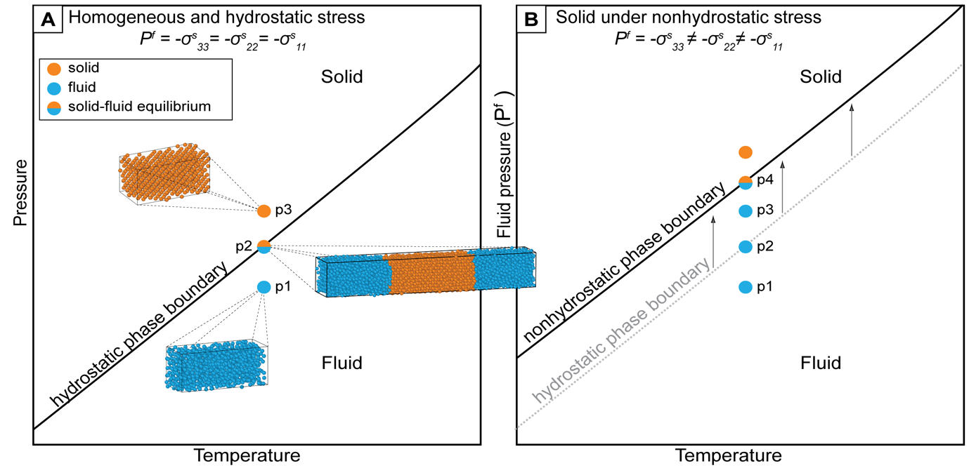
For a solid phase coexisting with a fluid of the same component, the hydrostatic equilibrium is achieved when the system, which is kept under a uniform hydrostatic pressure $P_{H}$, reaches the corresponding temperature $T_{H}$ on the solid-fluid thermodynamic phase boundary (fig. 4A). However, the direct assessment of the thermodynamic equilibrium by MD simulations is often challenging, since the melting/crystallization process is a first order phase transition and the energy barriers may induce appreciable kinetic effects, i.e., deviations from thermodynamic equilibrium.

Figure 4.Schematic representation of solid-fluid equilibrium in a $P-T$ diagram. (A) The $P,T$ points at which the solid and the fluid coexist at equilibrium under a homogeneous and hydrostatic stress state define the usual hydrostatic phase boundary in the $P-T$ space. Examples of snapshots of the atomic configuration of the LJ fluid (p1) and fcc solid (p3) phases, and of the solid-fluid coexistence at equilibrium (p2) as calculated from MD are shown. Atoms belonging to the solid and fluid phases (see appendix C) are shown in orange and blue, respectively. The rendering was performed using the OVITO software (Stukowski, 2010). (B) When the solid is stressed in a nonhydrostatic manner, the equilibrium between the solid and the fluid is achieved at a fluid pressure $P^{f}$ higher than the pressure on the hydrostatic boundary at the same temperature (e.g., p2 in A and p4 in B). For a fixed stress state of the solid, the variation of the equilibrium $P^{f}$ with temperature would define a nonhydrostatic phase boundary that is shifted to higher pressures (and lower temperatures) compared to the hydrostatic boundary. Therefore, a solid can be melted under nonhydrostatic stress conditions because of the shift of the phase equilibria (e.g., p2 is a coexistence state in A but it melts in B).

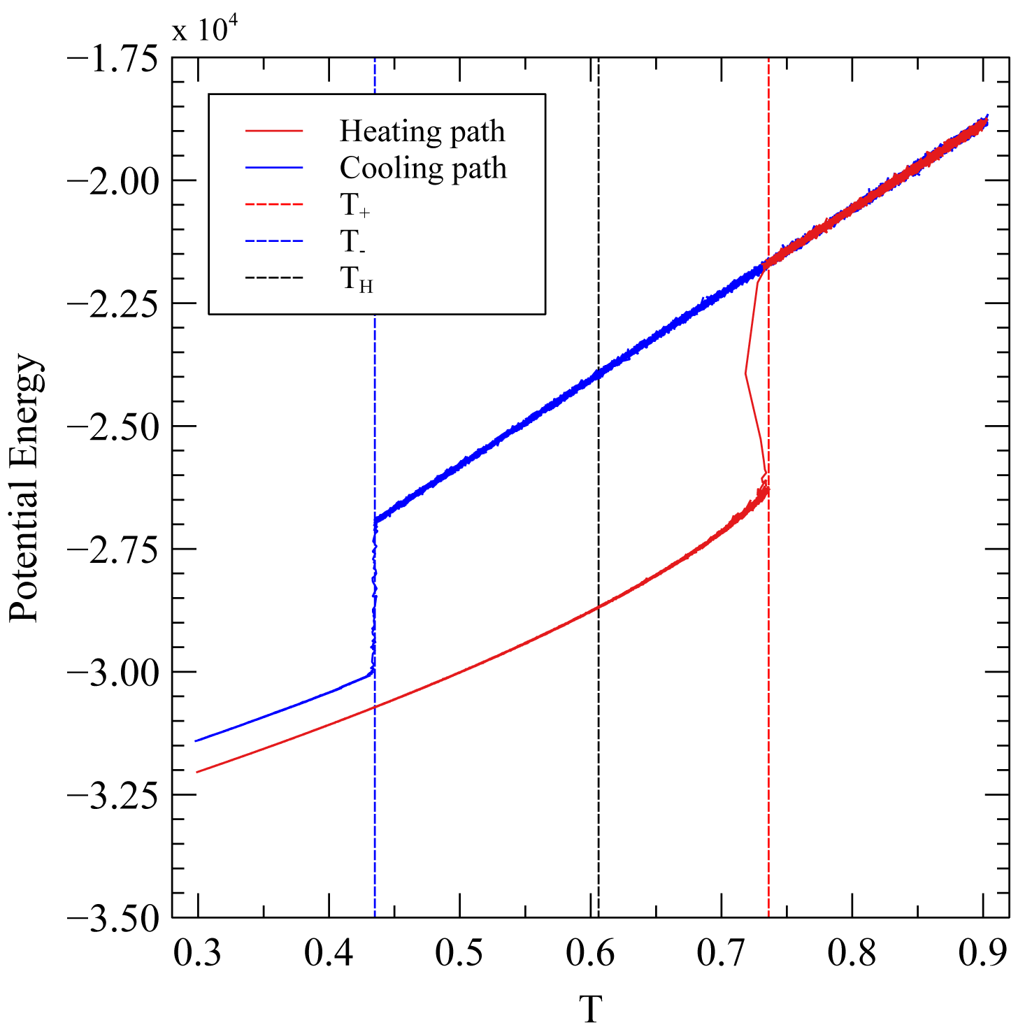
To obtain an initial estimate of the melting temperature at a given pressure $P_{H}$, we performed nonequilibrium melting and crystallization MD simulations following the hysteresis method (Luo et al., 2004). To this aim we first create an initial configuration corresponding to a homogeneous solid LJ material by placing the atoms on the nodes of a cubic fcc crystal lattice. The unit cell is replicated 6 times along $x_{1}$ and $x_{2}$ and 36 times along $x_{3}$, and contains a total of 5184 atoms. The boundary conditions of the MD simulations are periodic along $x_{1}$, $x_{2}$ and $x_{3}$. The simulation was performed in a $NPT$ ensemble (with constant properties at every timestep: $N$, number of particles; $P$, hydrostatic pressure; $T$, temperature). The homogenous crystal was heated incrementally at constant hydrostatic $P_{H}$ until complete melting, and then cooled to the initial temperature. The heating and the cooling have an equal duration and the T is varied following a linear ramp. The evolution of the energy ($E$) of the system as a function of T is discontinuous because of the latent heat of melting/crystallization (fig. 5). Since the kinetic barrier induces superheating and supercooling effects, the $T_{+}$ of complete melting and the $T_{-}$ of complete crystallization are not equal, and they can be determined from the hysteresis defined in the $E - T$ space (fig. 5). Following Luo et al. (2004), we determined from the hysteresis the equilibrium melting $T_{H}$ at hydrostatic conditions ($T_{H}$ = 0.606 in LJ reduced units, see fig. 5). However, such nonequilibrium approach does not provide us with a configuration of the system in which the solid and the fluid phases are coexisting in a stable equilibrium.

Figure 5.Potential energy-temperature hysteresis, generated by heating and cooling at constant rate in an $NPT$ ensemble for $30 \cdot 10^{6}$ timesteps at the hydrostatic $P_{H} = 0.5$. The $T_{+} = 0.737$ and $T_{-} = 0.435$ are found as the T of melting and crystallization, respectively. Because of the cooling rate and the effect of boundary conditions, defects are formed during the crystallization along the cooling path. Therefore, the solid formed from supercooled liquid has higher enthalpy than the initial solid, explaining the small difference in energy between the heating and cooling paths at $T < T_{-}$. The equilibrium temperature of melting at hydrostatic pressure $T_{H} = 0.606$ is calculated as described in Luo et al. (2004, eq. (14)). All quantities are reported as LJ reduced units.

In order to obtain an equilibrated and stable system with coexisting solid-fluid, we implemented the two-phase method in which the solid and fluid phases are kept in direct contact (Dozhdikov et al., 2012; Luo et al., 2004; Yoo et al., 2009). We used the same initial configuration as in the previous simulations with a solid supercell with 5184 atoms. The extension of the simulation block along the $x_{3}$ axis prevents phase boundary effects during the simulation (Noya et al., 2008). This solid system is equilibrated in an NPT ensemble at the hydrostatic pressure $P_{H}$ at a temperature $T_{s}$ below the equilibrium melting temperature $T_{H}$ that was estimated previously with the hysteresis method. The atoms in the simulation block are then grouped into three layers, each containing an equal number of atoms. The interfaces separating the layers are normal to the $x_{3}$ axis of the simulation block (fig. 3). The atoms of the central layer are kept “frozen”, at the temperature $T_{s}$, and therefore they remain in the solid state. The other two layers are heated up to a temperature $T_{m}$ above the $T_{+}$ determined from the hysteresis method. The heating is performed in a $NP_{x_{3}}AT$ ensemble (with constant: $N$, number of particles; $P_{x_{3}}$, total stress along the $x_{3}$ axis; $A$, area in the plane normal to $x_{3}$; $T$, temperature) which ensures that the total stress along the $x_{3}$ axis is kept close to the prescribed value $P_{H}$ during the entire heating (Yoo et al., 2004). The Steinhardt’s local bond-order parameters (Auer & Frenkel, 2005; Steinhardt et al., 1983) are determined from the coordinates of the atoms in order to assess for each individual atom whether it is in the solid (more ordered) or liquid state (less ordered). The details of the calculation of the order parameter are reported in appendix C. With this procedure, we can assess if the two lateral layers (fig. 3) are completely melted.

Then, the temperature of the molten layers is rapidly dropped to the level $T_{s}$ of the “frozen” solid layer in a $NP_{x_{3}}AT$ ensemble. At the final stage, the entire system composed of the coexisting solid and fluid layers is allowed to equilibrate. The equilibration is performed in the $NPH$ (i.e., constant particle number, hydrostatic pressure and enthalpy) ensemble by maintaining the prescribed $P_{H}$ and allowing all the sides of the simulation box to be adjusted independently in order to relax the anisotropic stress that might arise because of the initial small differences of temperature and stress between the solid and the fluid layers (Morris & Song, 2002; Yoo et al., 2009). During this final equilibration in the $NPH$ ensemble, the temperature is not constrained and evolves according to the energy and the configuration of the system. If the solid-fluid system is at $T$ higher than the melting $T$, the Gibbs free energy of the crystalline phase is higher than that of the liquid phase and the crystalline phase will melt due to absorption of heat, resulting in a decrease in kinetic $T$ of the system (Yoo et al., 2009). The opposite situation takes place if the $T$ of the system is lower than the melting $T$, leading to the crystallization of the melt and to the increase in the kinetic $T$ of the system.

The solid-fluid equilibrium is achieved when $T$ fluctuates around a constant mean value (i.e., the temperature distribution is Gaussian) in time. The number of solid and liquid atoms (as determined with the analysis in appendix C) must also remain steady in time, which indicates that the rate of melting and crystallization are equal. On the contrary, if the initial energy was too high or too low, the coexistence of the solid and fluid phases would not be stable, and it would lead to a complete crystallization or melting of the system. In this case, the procedure is repeated by varying the initial $T_{s}$ or $T_{m}$ to find a final state where both the solid and fluid are present and are in mutual equilibrium. When the coexisting system has reached equilibrium, the average pressure and temperature of melting $\left( P_{H},\ T_{H} \right)$ are calculated as the time-averages over a production run of 5$\ \cdot 10^{6}$ timesteps.

The $T_{H}$ = 0.60935 (15) (LJ reduced units) of equilibrium melting determined at $P_{H} = 0.5$ (LJ reduced units) with the two-phase methods agrees with the estimate obtained from the hysteresis method $(T_{H}$ = 0.606, LJ reduced units) to better than 0.5%, as expected for an equilibrated system (Luo et al., 2004). Moreover, as an independent benchmark of the reliability of this approach we used our simulation strategy to reproduce the equilibrium melting T reported in the literature for the standard LJ formulation (eq 15). Mastny and de Pablo (2007) calculated accurately the melting T (0.7793 ± 0.0004, LJ reduced units) at a pressure of 1 (reduced units) assuming an infinite-size and full-potential. By adopting the same standard LJ formulation, and a large cutoff distance of 10$b$ to approximate the full-potential, we obtained an equilibrium melting $T$ of 0.7787 ± 0.0003 at a pressure of 1 (reduced units), which closely approximates the results of Mastny and de Pablo (2007) despite the finite-size of our system.

4.2. Simulations under nonhydrostatic stress at constant temperature

The variation of the pressure of the fluid at equilibrium with a stressed solid was investigated in a series of simulations in which various strain states are applied to the solid. To this aim, the configuration obtained after the previous hydrostatic equilibration at $T_{H},\ P_{H}$ (tables 2, 3) was used as the initial configuration. During the equilibration in the $NPH$ ensemble discussed above, the lateral dimensions of the simulation box are adjusted independently, and they fluctuate randomly around their equilibrium value under hydrostatic pressure. Therefore, the sides ${lx}_{1}$ and $lx_{2}$ of the LJ solid (along $x_{1}$ and $x_{2}$ , respectively) in the final configuration may have a small difference (less than 0.03%), which results in a small virtual lateral strain of the solid. In order to have a reference configuration with a completely laterally unstrained solid, we fix ${lx}_{1}$ = $lx_{2}$ and perform a further isothermal equilibration in the canonical ($NVT$, constant number of particles, volume and temperature) ensemble by employing a Nosé–Hoover thermostat (Shinoda et al., 2004) at the equilibrium $T_{H}$ = 0.60935. The final configuration (shown in fig. 3A) still preserves the solid-fluid equilibrium at hydrostatic conditions, and the stress of the system is calculated as time-averages during a production run of 50 $\cdot 10^{6}$ timesteps (table 2).

To generate the nonhydrostatic stress states in the solid, the previous hydrostatic configuration was subject to lateral tensile or compressive strains parallel to the $x_{1}$ and $x_{2}$ coordinate axes that are normal to the “free” surfaces of the solid, by scaling the respective dimensions of the box. The $x_{3}$ dimension is left unchanged since the stress in this direction will be determined by $P^{f}$. During this loading, the volume of the solid may change in response to the applied strain, and it is not constrained in the simulation (see section 5 for a discussion on the evolution of the mean stress of the solid under stress). Upon loading, the applied compressive or tensile strain determines an initial increase or decrease of the $P^{f}$, respectively. At the same time, a nonhydrostatic stress is developed in the solid phase due to the applied strain. However, such virtual configuration is not in equilibrium since the stress component of the solid normal to the solid-fluid interface $(\sigma_{33}^{s}$ in fig. 3) may not be equal to the $- P_{f}$, as would be expected from force balance. An isothermal equilibration was therefore performed in the $NVT$ keeping the new $x_{1},$ $x_{2}$ and $x_{3}$ dimensions of the simulation box and the $T_{H}$ constant, for 50 $\cdot 10^{6}$ timesteps.

At this point we would like to point out that with MD simulations the equilibration is not found by imposing a specific thermodynamic relationship, such as that of equation (4). Instead, the equilibration is achieved by letting the trajectories of the atoms evolve in response to their potential and kinetic energy, which are in turn affected by the prescribed strain and temperature conditions. This results in the spontaneous crystallization or melting of a limited amount of material due to difference in energy between the solid and fluid phases in the strained system. The atomic volume of the LJ fcc solid is smaller than that of the liquid (table 2). During the equilibration in the $NVT$ ensemble, the crystallization of part of the fluid or the melting of part of the solid leads to a decrease or increase of the $P^{f},$ respectively. The stress state of the solid also varies in response to its own crystallization/melting and to the variation of the $P^{f}$. If the equilibrium is restored at the prescribed strain conditions, the stress component $\sigma_{33}^{s}$ becomes equal to the $- P^{f}$ and the energy configuration of the atoms in the two phases counteracts further crystallization or melting.

After the equilibration is achieved, a 50 $\cdot 10^{6}$ timesteps production run is performed to compute the resulting equilibrium $P^{f}$ and to produce the snapshots with the per-atom positions and stresses required to calculate the order parameters (appendix C) and the stress of the solid layer (calculate as described in appendix D) in the post-processing. For each simulation, the pressure of the fluid and the stress of the solid in the equilibrium stage were computed as ensemble averages and are reported in table 4.

5. SOLID-FLUID EQUILIBRIUM AT NONHYDROSTATIC CONDITIONS ASSESSED BY MOLECULAR DYNAMICS SIMULATIONS

For a solid-fluid system at hydrostatic conditions, all the $P,T$ points at which the solid and the fluid phases coexist in thermodynamic equilibrium define the usual thermodynamic phase boundary in $P - T$ space (e.g., fig. 4A). As discussed above, equation (14) describes the expected variation of the equilibrium $P^{f}$ when a single-component solid-fluid system is taken from a hydrostatic equilibrium to a nonhydrostatic state at constant temperature. According to equation (14), the pressure of a fluid in equilibrium with a nonhydrostatic solid is expected to be always higher than the pressure of the same fluid equilibrated with a hydrostatic solid due to the positive contribution of deviatoric stress to the specific Helmholtz energy of a solid. As a consequence, the equilibrium phase boundary, defined by all the $P^{f},\ T$ points representing the pressure of the fluid in equilibrium with the stressed solid at varying temperature, would always be shifted to higher pressures (and lower temperatures) compared to the hydrostatic (classic) phase boundary (fig. 4B).

In order to confirm quantitatively the magnitude of the change in equilibrium fluid pressure and the mean stress of the solid under various nonhydrostatic stress conditions, we performed several atomistic MD simulations by adopting the procedure outlined above. Compared to the previous study by Frolov and Mishin (2010), we investigated the conditions of nonhydrostatic equilibria under large (non-zero) initial pressure. In our simulations we assume that the strain along the $x_{1}$ and $x_{2}$ coordinate axes are always equal one another $(\varepsilon_{11} = \varepsilon_{22}$) with no shear components. We define the resulting strain configuration as axially-symmetric (fig. 3B). As will be discussed later, such a configuration produces a volume strain in the solid phase. Because the internal pressure of the fluid phase is independent of the shape of the simulation cell, the stress state of the fluid is hydrostatic in the entire range of deformation. On the other hand, the applied axially-symmetric strain together with the chosen orientation of the solid (fig. 3) induces a nonhydrostatic stress in the solid with equal lateral stress components $\left( \sigma_{11}^{s} = \sigma_{22}^{s} \right)$, which are aligned along the $x_{1}$ and $x_{2}$ axes of the simulation cell. Because of the previous relation, we have the following equality between the $q_{11}^{s}$ and $q_{22}^{s}$ tensor components: $q_{11}^{s} = \ \sigma_{11}^{s} + P^{f} = q_{22}^{s} = \sigma_{22}^{s} + P^{f}$ . Finally, the mechanical equilibrium along the $x_{3}$ direction imposes that $\sigma_{33}^{s} = - P^{f}$ and, since the principal axes of strain and stress coincide with the coordinate axes, the shear components are zero ($q_{ij} = 0$ when $i \neq j$).

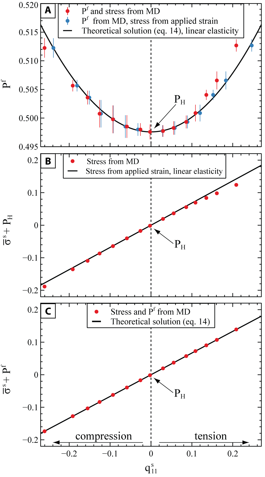
The results of the MD simulations (fig. 6A) confirm that the $P^{f}$ at equilibrium increases for any stress state of the solid away from the initial hydrostatic reference pressure $P^{H}$. Figure 6B shows that also the $\overline{\sigma^{s}}$ varies from the initial hydrostatic pressure when a nonhydrostatic stress is applied to it. This is expected, because of the strain field used in our simulations ${(\varepsilon}_{11} = \varepsilon_{22})$, combined with the crystallographic symmetry and orientation of the solid, which results in a volumetric strain of the solid. At the maximum deformation explored in our simulations, the variation of $\overline{\sigma^{s}}$ with respect to the initial hydrostatic $P_{H}$ ($\approx$ 37%, fig. 6B) is one order of magnitude larger than the variation of the $P^{f}$ $( \approx$ 2.8%, fig. 6A). Moreover, when the solid is placed under nonhydrostatic conditions, its “pressure” (i.e., $- \overline{\sigma^{s}}$) is decoupled from the pressure of the fluid $P^{f}$ with which it is in thermodynamic equilibrium and can deviate largely from it (fig. 6C).

Figure 6.Results of MD simulations as a function of the nonhydrostatic stress applied to the solid, with components $q_{11}^{s} = q_{22}^{s}$ (fig. 3B, table 4) at a constant temperature $T_{0} = 0.60935$ (LJ reduced units). (A) Pressure of the LJ fluid at nonhydrostatic equilibrium. (B) Deviation of the mean stress $(\overline{\sigma^{s}})$ of the nonhydrostatic LJ solid layer from its initial mean stress $( - P_{H})$ at hydrostatic equilibrium. (C) Deviation of $\overline{\sigma^{s}}$ from the negative of the equilibrium pressure ${( - P}^{f})$ of the fluid. The solid lines in (A) and (C) are calculated from equation (14) using the properties at hydrostatic conditions reported in tables 2 and 3. The $\overline{\sigma^{s}}$ along the solid line in (B) is calculated from the strain applied to the solid and the ${- P}^{f}$, using linear elasticity (elastic properties in table 3). All the stress and pressure quantities are reported as LJ reduced units.

The solid line shown in figure 6A represents the $P^{f}$ calculated from equation (14) using the elastic constants determined on our solid at the hydrostatic reference state (tables 2 and 3). A very good agreement is found between the theoretical solution (eq. 14) and the results of our MD simulations under small deformations (fig. 6A). The deviations observed under large deformations are due to the assumption of linear elasticity in the derivation equation (14), which assumes that the deformations are small and neglects the variation of the elastic properties of the solid with stress. Therefore, the analytical solution (eq. 14) does not account for the stiffening of the solid under compressive deformations, nor for its softening under tensile stress. As a consequence, it underestimates the value of stress (and therefore of $q_{11}^{s}$) in compression, while it overestimates it in tension. This is also reflected in Fig. 6B, which shows that by using constant elastic properties (solid line), the variation of $\overline{\sigma^{s}}$ is underestimated under compression and overestimated under tension.

To further investigate this effect, for each simulation we used linear elasticity to recalculate the “linearized” stress of the solid, by knowing the components $\varepsilon_{11}$ and $\varepsilon_{22}$ of the applied strain and imposing that, because of mechanical equilibrium, $\sigma_{33}^{s} = {- P}^{f}$(fig. 3). Figure 6A shows an excellent agreement of the recalculated points with the predictions of the analytical solution (blue dots in fig. 6A), confirming that the small deviations with respect to our MD results are due to the assumptions of small strains behind equation (14). However, the errors of the analytical solution on the determination of $P^{f}$ are less than 1% even at the largest deformation, despite the very large differential stress of the solid ($\approx 50\%$ of the initial hydrostatic pressure) at these conditions.

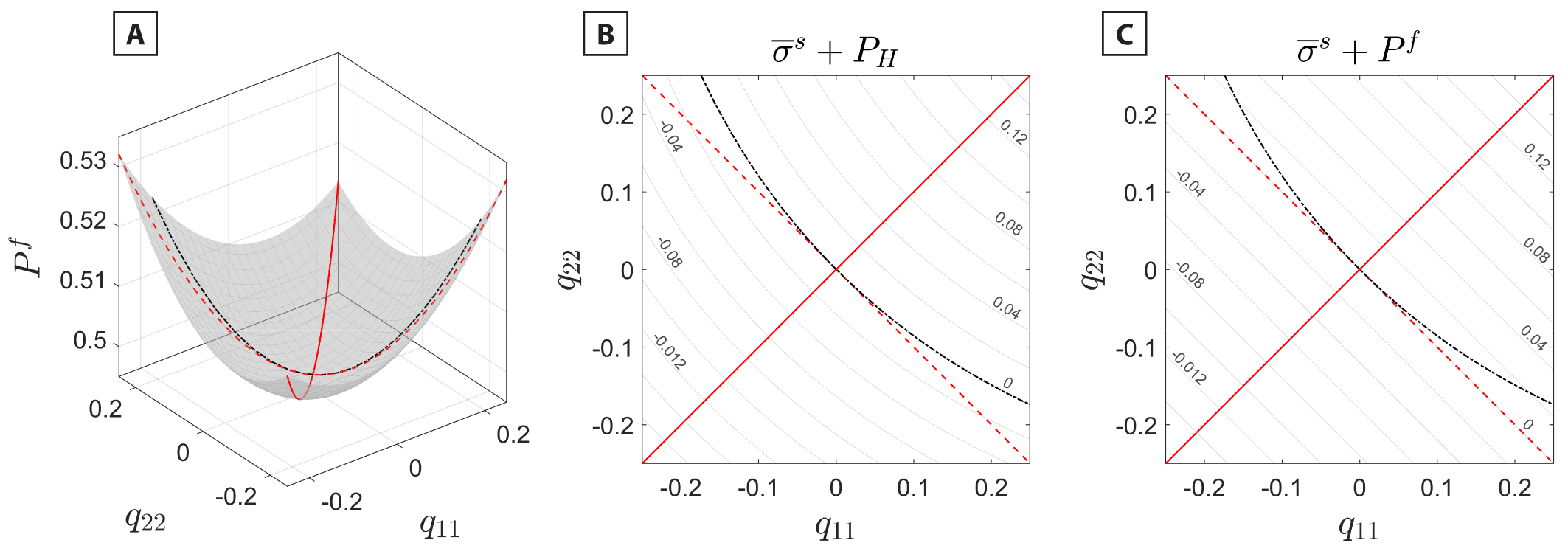
We note that not all of the possible strain configurations lead to the same evolution of $P^{f}$, and to the same deviation of $\overline{\sigma^{s}}$ from $- P_{H}$ and $- P^{f}$, as those shown in figure 6. Figure 7 shows these equilibrium quantities as obtained from the theoretical relationship of equation (14), by varying $q_{11}$ and $q_{22}$ independently. In our simulations we explored the path with $q_{11} = q_{22}$ (solid red line in fig. 7A, B, C). This path produces the largest deviation of the $\overline{\sigma^{s}}$ from the reference pressure $P^{H}$ (fig. 7B) and from $P^{f}$ (fig. 7C). Since $\overline{\sigma^{s}} = \frac{q_{11} + q_{22} - \ 3P^{f}}{3}$, the $\overline{\sigma^{s}}$ remains equal to ${- P}^{f}$ only when $q_{11} = \ {- q}_{22}$ (red dashed line in fig. 7C). Because $\overline{\sigma^{s}} = {- P}^{f}$ along this particular path, the tensor $q_{ij}^{s} = \ \sigma_{ij}^{s} + \delta_{ij}P^{f}$ is equal to the deviatoric stress of the solid. With our choice of crystallographic orientation of the solid, and since the LJ fcc solid has a cubic crystallographic symmetry, $\overline{\sigma^{s}}$ stays equal to ${- P}^{f}$when the applied strain has components $\varepsilon_{11} = \ - \varepsilon_{22}$. However, even this strain configuration induces a volume strain of the solid phase with respect to the initial hydrostatic reference state at $P^{H}$, and therefore a variation of its $\overline{\sigma^{s}}$ (red dashed line, fig. 7B). This is due to the fact that, despite $\varepsilon_{11} = \ - \varepsilon_{22}$, the normal strain component along the third direction ($\varepsilon_{33}$) is controlled by the equilibrium $P^{f}$, which varies in response to the strain applied to the solid (fig. 7A). A more complex path in $q_{11}$ and $q_{22}$ can be found that maintains the $\overline{\sigma^{s}}$ equal to the initial $- P_{H}$ (black dash-dotted line, fig. 7B). However, along this path the $\overline{\sigma^{s}}$ does not equal the equilibrium ${- P}^{f}$ in the stressed system (black dash-dotted line, fig. 7C).

Figure 7.Equilibrium quantities of the LJ system under nonhydrostatic stress, as obtained from the theoretical relationship of equation (14) by varying the components $q_{11}$ and $q_{22}$ independently. (A) Variation of the equilibrium pressure of the fluid $P^{f}$ with stress (grey surface). (B) Deviation of the mean stress $(\overline{\sigma^{s}})$ of the nonhydrostatic solid layer from its initial mean stress $( - P_{H})$ at hydrostatic equilibrium, shown as contours. (C) Deviation of $\overline{\sigma^{s}}$ from the negative of the pressure of the fluid ${( - P}^{f})$ at nonhydrostatic equilibrium, shown as contours. Three deformation paths are shown as lines. Red solid line: path with $q_{11} = q_{22}$, as explored in our MD simulations (see fig. 6). Red dashed line: path with $q_{11} = {- q}_{22}$; along this path the $\overline{\sigma^{s}}$ = ${- P}^{f}$ (C), but deviates from the initial $- P_{H}$ (B). Black dashed line: path along which the $\overline{\sigma^{s}}$ = $- P_{H}$ (B), but deviates from ${- P}^{f}$ (C). All the shown stress and pressure quantities are reported as LJ reduced units. The properties used in the calculations are reported in tables 2 and 3.

6. DISCUSSION

6.1. Equilibrium pressure of mineral phases in equilibrium with their melt under nonhydrostatic conditions

The results of our MD simulations reported in fig. 6A show that the theoretical relationship based on linear elasticity (eq 14) describes correctly the change of the fluid-solid equilibrium pressure up to compressions and tensions with a $q_{11}^{s} = q_{22}^{s}$ of at least ± 20% of the initial pressure at hydrostatic conditions. Therefore, we applied this theory to calculate the equilibrium pressure between several solid mineral phases ($Mg_{2}SiO_{4}$, forsterite; $SiO_{2},$ quartz; $NaCl$, halite) and their pure melt. Initially the mineral-melt equilibrium is evaluated at hydrostatic conditions. Since each of these systems reaches the solid-melt equilibrium at different P and T conditions, in order to compare consistently their behavior, we introduce a nondimensional pressure defined as the pressure $P_{H}$ at which a solid phase reaches the hydrostatic equilibrium with its pure melt at a given $T_{H}$, normalized over the bulk modulus (K) of the solid phase at that $P_{H},T_{H}$. For the LJ system at the hydrostatic conditions $P_{H},T_{H}$ of our simulations, the nondimensional hydrostatic equilibrium pressure is $P^{'} = \frac{P_{H}}{K} = 0.0253$ (table 3). We used the Perple_X software (Connolly, 2005, 2009) with data from the Holland and Powell (2011) thermodynamic database to map the variation in the P-T space of the nondimensional solid pressure $P^{'} = \frac{P}{K}$ for each mineral phase. Then, in order to compare the solid-melt equilibrium pressure of all the systems, we found for each of them the $P$ and $T$ condition along their melting line where the condition $P^{'} = \ 0.0253$ is satisfied. The $P$ and T of hydrostatic solid-melt equilibrium obtained in this way for each phase are reported in table 5, and they are used as reference states to evaluate the perturbation due to nonhydrostatic stress.

Since the anisotropic properties of these mineral phases are not available at the required P and T conditions, we used their isotropic properties calculated from the Perple_X software (Young’s modulus and Poisson’s ratio, table 5) together with equation (B2) to investigate the variation of the equilibrium pressure of the melt expected from the application of a nonhydrostatic stress to the solid mineral. We applied an axially-symmetric strain state as in the MD simulations (i.e., $\varepsilon_{11} = \varepsilon_{22}$, and no shear components) assuming the same orientation of the Cartesian axes as in figure 3. Since the minerals are assumed to be elastically isotropic, the exposition of the solid layer to these lateral strains along the $x_{1}$and $x_{2}$ directions and to the $P^{f}$ along the $x_{3}$ direction, results in a nonhydrostatic stress in the solid with $q_{11}^{s} = q_{22}^{s}$ (i.e., the same path as the solid red line in fig. 7).

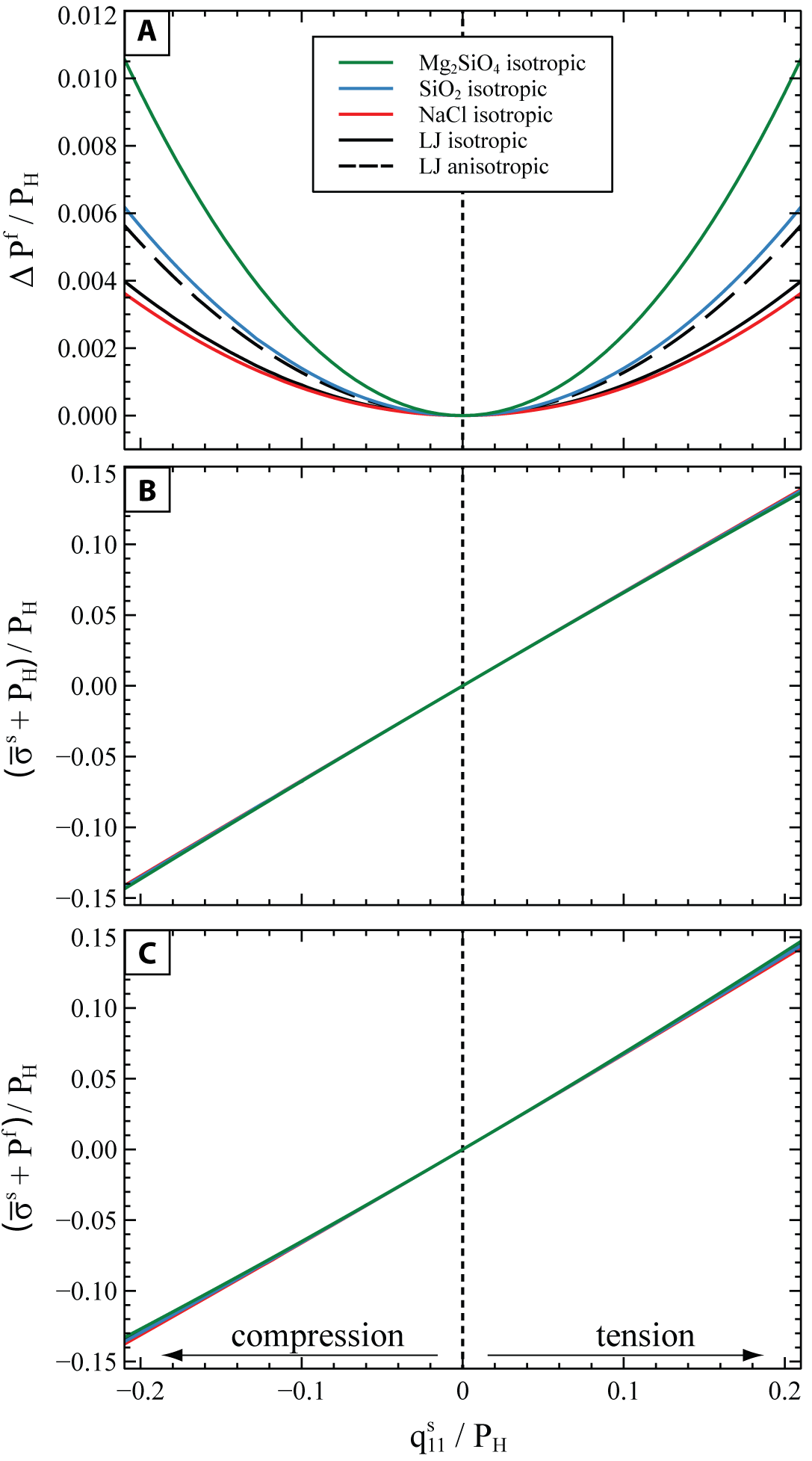
Figure 8 shows the change in the equilibrium $P^{f}$ and in the $\overline{\sigma^{s}}$ for a nonhydrostatic compression and tension up to ± 20% of the initial hydrostatic pressure. In order to compare the results obtained for minerals at solid-melt equilibrium at different $P$ and $T$, for each system the applied nonhydrostatic stress and the variations in $P^{f}$(fig. 8A) and $\overline{\sigma^{s}}$ (fig. 8B, C) are all normalized to the initial $P_{H}$ of the system.

Figure 8.Melt-solid equilibrium as a function of the nonhydrostatic stress applied to the solid with components $q_{11}^{s} = q_{22}^{s}$ at constant $T$. The initial hydrostatic $P_{H}$, $T_{H}$ conditions of $Mg_{2}SiO_{4}$ $(2.70 \ \text{GPa}, 2304 \ \text{K})$, $SiO_{2}$ $(1.49 \ \text{GPa}, 2262 \ \text{K})$,$\ NaCl$ $(0.95 \ \text{GPa}, 1264 \ \text{K})$ and the LJ material $(0.5 \varepsilon/\sigma^{3}, 0.609 \varepsilon/k_{B}$) are determined from their respective melt lines at the nondimensional pressure $P^{'} = P/K = 0.0253$, as explained in the main text. All of the quantities are normalized on the initial hydrostatic $P_{H}$ of the system. (A) Variation of the melt equilibrium pressure calculated from equation (B2) assuming isotropic elastic properties for the solid. The dashed line (anisotropic LJ) has been calculated with equation (14) assuming anisotropic elastic properties for the solid. (B) Deviation of the mean stress $(\overline{\sigma^{s}})$ of the nonhydrostatic solid layer from its initial mean stress $( - P_{H})$ at hydrostatic equilibrium. (C) Deviation of $\overline{\sigma^{s}}$ from the negative of the equilibrium pressure ${( - P}^{f})$ of the fluid. The properties of each phase at hydrostatic conditions are reported in tables 2, 3 and 5.

Figure 8A shows that for all the investigated minerals, the equilibrium pressure of the melt increases for any compressional or tensile stress state of the solid. In general, the equilibrium melt pressure increases more in systems in which the solid phase is stiffer. Indeed, solids that are elastically stiffer store more elastic energy for the same amount of applied strain (eq 8). Therefore, in order to preserve the solid-melt equilibrium in systems with a stiffer solid phase, the pressure of the melt must also increase for the chemical potential of the melt ($\mu^{f}$) to keep up with the increase in Helmholtz energy of the solid (see eq 10). Moreover, figure 8A shows a difference in the change of the equilibrium $P^{f}$ for the anisotropic and isotropic LJ, calculated respectively with equations (14) and (B2). The discrepancy between the isotropic and anisotropic curves can be estimated from equation (B3), which shows that for the LJ material the change in the $P^{f}$ is underestimated by $\approx$29% when using isotropic elastic properties. This is due to the LJ solid being highly anisotropic, with a universal anisotropic index (Ranganathan & Ostoja-Starzewski, 2008) $A^{U} = 1.73$ (for reference, an isotropic solid would have $A^{U} =$ 0). The anisotropic calculation cannot accurately be performed for the other phases, since their anisotropic elastic constants at the chosen melting conditions are not available. However, we can roughly estimate the discrepancy between the anisotropic and the isotropic solution, by evaluating equation (B3) at ambient conditions (1 bar, 298K) and assuming that this discrepancy stays constant at increased P and T conditions.

For example, for quartz (anisotropic index $A^{U} = 1.30$ at room conditions), the isotropic approximation underestimates the equilibrium pressure by $\approx$ 27% when using the anisotropic elastic properties of quartz from ambient conditions (cf. Lakshtanov et al., 2007). However, even allowing for the contribution of elastic anisotropy, the change in the normalized melt-solid equilibrium pressure $(\Delta P^{f}/P_{H}$) would still be at least one order of magnitude less than the applied normalized nonhydrostatic stress ($q_{11}^{s}/P_{H}$). On the other hand, the normalized variation of the mean stress of the solid $(\overline{\sigma^{s}} + P_{H})/P_{H}$; fig. 8B) is of the same order of magnitude as the applied normalized nonhydrostatic stress ($q_{11}^{s}/P_{H}$). Under this deformation, the $\overline{\sigma^{s}}$ also deviates substantially from the $- P^{f}$ of the fluid to which it is in equilibrium with (fig. 8C).

6.2. Implications for solid-fluid multiphase systems in porous rocks

As shown in figure 2 and discussed above, pressure gradients are expected in multiphase systems when solid minerals are in direct contact with fluids, even under static conditions and without external tectonic stresses. While fluid will always experience a hydrostatic stress gradient (fig. 2A), solid grains will experience nonhomogeneous and nonhydrostatic stress (fig. 2B, C) due to the changes in the contact area between the grains and the requirements imposed by mechanical equilibrium. Therefore, nonhydrostatically stressed minerals and hydrostatic fluids can coexist, a condition that breaks the fundamental assumption behind the use of Gibbs potentials to describe reactions in such solid-fluid systems. With MD simulations we can quantify the magnitude of the errors expected if a hydrostatic Gibbs potential is used to describe phase equilibria between a fluid and a solid for nonhydrostatic conditions. Our results are in agreement with previous theory (Frolov & Mishin, 2010; Gibbs, 1876; Sekerka & Cahn, 2004), and confirm that for single component systems, the equilibrium pressure of the fluid changes quadratically with the nonhydrostatic stress applied to the solid matrix (fig. 6).

However, for the nonhydrostatic stresses expected in the lithosphere (with differential stresses of several hundreds of MPa; Andersen et al., 2008; Brace & Kohlstedt, 1980; Kiss et al., 2023; Prieto et al., 2012), the variation of the equilibrium pressure of the fluid, and therefore the displacement of the thermodynamic pressure of phase equilibria, is almost negligible. For example, we can consider the worst case among those reported in figure 8A of a forsterite in hydrostatic equilibrium with its pure melt at a pressure of 2.7 GPa and temperature of 2304 K (table 5). For an applied axially-symmetric nonhydrostatic stress with $q_{11}^{s} = q_{22}^{s} =$ ± 0.5 GPa, the equilibrium pressure of the melt increases by 0.02 GPa, i.e., an increase of less than 1% with respect to the initial pressure in the purely hydrostatic system. This implies that, for cases similar to ours, the pressure of a melt that is in thermodynamic equilibrium with a nonhydrostatically stressed solid is close to melt pressure at the hydrostatic limit. Therefore, the thermodynamic pressure that controls the solid-melt equilibria is equal to the pressure of the fluid, which remains almost constant even when a differential stress is applied to the solid matrix. This has relevant implications for models that describe multiphase systems under deformation, since, as a first approximation, they can use the pressure of the melt in a standard hydrostatic thermodynamic model (e.g., Perple_X software; Connolly, 2005, 2009) in order to estimate the phase equilibria of the stressed system.

However, it is important to note that when the system is under nonhydrostatic stress, even at thermodynamic equilibrium, the pressure of the melt $P^{f}$ may not be equal to the “pressure” of the solid (i.e. -$\overline{\sigma^{s}})$, and their deviation is often non negligible (fig. 6C, 7C, 8C). Therefore, in a stressed system, the use of the solid “pressure” instead of the fluid pressure to calculate the equilibrium assemblages may lead to large errors. As an example, we use once again the $Mg_{2}SiO_{4}$ system with an initial hydrostatic solid-melt equilibrium at 2.70 GPa and 2304 K. When an axially-symmetric nonhydrostatic stress $q_{11}^{s} = q_{22}^{s} = -0.5$ GPa is applied, the $P^{f}$ at thermodynamic equilibrium becomes 2.72 GPa, i.e., close to its value at the initial hydrostatic equilibrium. However, the solid “pressure” reaches 3.04 GPa (i.e., $\approx + 13\%$ variation) in the same deformation, and diverges significantly from the $P^{f}$.

The deviation of the $\overline{\sigma^{s}}$ from the $P^{f}$ with increasing applied stress in porous systems (fig. 2A and B), has important implications for understanding the interactions between fluids and rocks under deformation. In current hydro-mechanical-chemical (HMC models (e.g., Schmalholz et al., 2020), the density and the energy of the solid matrix are approximated using the values of the $P^{f}$. This is justified when the difference between the $\overline{\sigma^{s}}$ and the $- P^{f}$ is small. However, since nonhydrostatic stress can be developed in the solid matrix in such systems, the use of ${- P}^{f}$ as a proxy of $\overline{\sigma^{s}}$ can lead to inaccurate estimates of the density of the solid, even when the solid and the fluid are in thermodynamic equilibrium. The magnitude of such errors must be assessed on a case-by-case basis, because they depend on the specific deformation applied to the system (fig. 7C).

7. CONCLUSIONS

The interpretation of phase equilibria and reactions in geological materials has long been approximated by standard thermodynamics which assumes that the stress in the systems is hydrostatic and homogeneous (i.e., the same for all the phases involved). However, stress gradients and nonhydrostatic stresses are common in rocks and can occur even in porous systems with coexisting solid minerals and fluids (e.g., fig. 2). Currently there is still no accepted theory that extends thermodynamics to include the general effects of nonhydrostatic stress on reactions, and the use of several thermodynamic potentials in stressed geological system is still debated.

By means of MD simulations, we have investigated the effect of a homogeneous nonhydrostatic stress on the equilibrium between a solid and its pure melt. The advantages of this approach are: (i) the stress of the solid phase can be kept homogeneous. Therefore, the direct effect of a homogeneous, nonydrostatic stress on thermodynamic equilibria can be assessed, and the indirect perturbations due to local stress concentrations, that may be present in experiments, are avoided. (ii) It can be used to explore the equilibration of fluid-solid systems under known and controlled strain/stress states. (iii) The energy of the system and the local stress are monitored simultaneously while the system evolves toward equilibrium. (iv) It intrinsically accounts for the elastic anisotropy of the solid phase. (v) The equilibrium condition can be defined without any a priori assumptions of a specific thermodynamic theory. Such an approach is therefore extremely useful to validate the applicability of existing thermodynamic theories.

Our MD simulations show that for small applied strains, the equilibrium pressure of the fluid increases quadratically with the nonhydrostatic stress generated in the solid. These findings agree with the existing thermodynamic theory for single component systems (Frolov & Mishin, 2010; Gibbs, 1876; Sekerka & Cahn, 2004) and extend previous MD simulations performed at zero initial pressure (Frolov & Mishin, 2010).

We then use the analytical relationship derived by Sekerka and Cahn (2004) to explore the equilibrium between common mineral phases and their pure melts at the differential stresses expected in the lithosphere. We observe that, by applying an axially-symmetric load, the $P^{f}$at equilibrium increases by less than 1% even when the solid matrix is subject to a differential stress that is 20% above (compression) or below (tension) the initial hydrostatic pressure. However, the variation of the $\overline{\sigma^{s}}$ is one order of magnitude larger than the variation of $P^{f}$ under these stress conditions (fig. 8). In general, a decoupling of the “pressure” of the solid ($- \overline{\sigma^{s}}$) from the pressure of the fluid $P^{f}$ at the thermodynamic equilibrium is expected whenever the solid is put under a nonhydrostatic stress (fig. 7C). This has important implications for hydro-mechanical-chemical (HMC) models that describe the interactions between fluids and minerals under deformation. Our results imply that, at least for simple single-component porous systems, phase equilibria can be accurately predicted by taking the $P^{f}$ as a proxy of the equilibration pressure and assuming that it is not perturbed significantly by the typical levels of differential stress expected in the solid matrix in such systems (fig. 2). Despite the fact that the $\overline{\sigma^{s}}$ can deviate substantially from the $P^{f}$ in stressed systems, $\overline{\sigma^{s}}$ still remains a valuable thermodynamic quantity that is required for the accurate calculation of density and energy of the solid phase.

Our preliminary MD simulations at high pressure and temperature conditions show that this approach can provide quantitative estimates on the direct effect of nonhydrostatic stresses on phase equilibria and reactions in multiphase systems at geologically relevant conditions. While experimental studies of multicomponent systems suggest a significant role of the $P^{f}$ (e.g., Llana-Fúnez et al., 2012), a complete thermodynamic description of such systems under stress is still lacking. In this respect, our framework may be extended to real mineral systems by adopting appropriate force fields for geological materials. While our analysis does not take into account the effect of stress heterogeneities in the sample at larger scales, which can indirectly affect phase equilibria, the knowledge of the direct effect of deviatoric stress on thermodynamic equilibria gained from MD simulations can be incorporated into chemical-mechanical models that describe macroscopic geological systems under deformation.

ACKNOWLEDGEMENTS

All the authors acknowledge the Mainz Institute of Multiscale modelling (M³ODEL) for providing funding at the early parts of this research. M.L.M. was supported by an Alexander von Humboldt research fellowship. Boris Kaus received funding from the European Research Council (ERC) under the European Union’s Horizon 2020 research and innovation program (ERC CoG grant agreement No 771143 – MAGMA). We thank M. Alvaro, R.J. Angel, M. Prencipe and two anonymous reviewers for constructive comments that allowed us to improve this manuscript. The editorial handling and insightful comments by M. Brandon and A. Smye are greatly appreciated.

AUTHOR CONTRIBUTIONS

All authors contributed to the development of the ideas and writing of the manuscript. M.L.M and T.S. developed the strategy for the molecular dynamics simulations. M.L.M performed the molecular dynamics simulations and the post-processing. E.M. provided the calculation shown in figure 2. M.L.M, E.M. and B.K. derived the geological implications.

DATA AVAILIBILITY

All the sources of the data used are explicitly mentioned in the text.

Editor: Mark T. Brandon, Associate Editor: Andrew Smye

APPENDICES

APPENDIX A
Modelling the distribution of stress in granular rocks

In our model we consider a rock that is composed of two-media (solid-fluid) that have an effective viscosity ratio $\eta^{s}/\eta^{f}\ = 10^{4}$. We chose this ratio as an approximation since larger contrasts in effective viscosity do not affect the magnitude of pressure variations significantly (Moulas et al., 2014; Schmid & Podladchikov, 2003). Both the solid and the fluid are treated as isotropic and incompressible. The incompressible approximation leads to identical results to the compressible case for timescales that are ~ 10 times larger than the Maxwell viscoelastic timescale (Moulas et al., 2019). The Maxwell timescale is defined here as $t = \eta/K$, where $\eta$ is the effective viscosity and $K$ is the bulk modulus of the material. Finally, we would like to note that the viscous incompressible solution is mathematically equivalent to the elastic incompressible solution if one replaces viscosities by shear moduli and velocities by displacements (Goodier, 1934). Thus, we provide the viscous solution as a suitable approximation for the development of stresses over large timescales, but the stress pattern would be identical if one considers a purely elastic rheology.

To calculate the stress pattern of figure 2 we solve the conservation of momentum for the case of slow viscous flow:

$$- \frac{\partial P}{\partial x_{j}} + \frac{\partial\tau_{ij}}{\partial x_{i}} + \rho g_{j} = 0 \tag{A1}$$

where $P$ is the mean stress, $\tau_{ij}$ are the components of the deviatoric stress tensor, $\rho$ is the density and $g_{j}$ is the component of gravity acceleration in the j^th direction. The components of the deviatoric stress tensor are found as:

$$\tau_{ij} = \mu\left( \frac{\partial V_{j}}{\partial x_{i}} + \frac{\partial V_{i}}{\partial x_{j}} \right) \tag{A2}$$

where $V$ represents the velocity. The incompressibility condition is given by equation (A3).

$$\frac{\partial V_{k}}{\partial x_{k}} = 0 \tag{A3}$$

The system of equations is solved in an iterative manner by introducing an artificial compressibility in equation (A3) and by utilizing a staggered, finite-difference numerical grid (Chorin, 1997; Virieux, 1986) under free slip boundary conditions. Our model was solved in dimensionless form using the vertical lengthscale ($L$), the lithostatic pressure ($\rho^{s}gL$), and the solid’s effective viscosity ($\eta^{s}$) as independent scales. To complete the solution, we have considered a density ratio $\rho^{s}/\rho^{f} = 2700/1000$.

Our system of equations was solved by using the pseudo-transient approach (Chorin, 1997; Duretz et al., 2019; Räss et al., 2022). However, we have modified the iteration strategy by imposing that the stress tensor within the fluid domains is given by the following relationships:

$$\sigma_{i j}=-P \delta_{i j}+\tau_{i j}=-\rho^f g(L-y) \delta_{i j}\tag{A4a}$$

$$\tau_{ij} = 0\tag{A4b}$$

where $\sigma_{ij}$ are the components of the total stress tensor and $\delta_{ij}$ is the Kronecker delta. The previous modification ensures that the fluid has zero deviatoric stress and its state of stress is hydrostatic as it would be the case if the porosity was interconnected.

APPENDIX B
Equilibrium between a fluid and an elastically isotropic solid under stress

Sekerka and Cahn (2004) obtained a relation equivalent to equations (13) and (14) for an elastically isotropic solid under stress in equilibrium with a fluid of the same component. Assuming that the shear stresses in the $x_{1}x_{2}$ plane are zero ($\sigma_{12} = 0$), they derived the following expression for the change of the equilibrium temperature of the system due to the application of a nonhydrostatic stress in the solid at constant pressure in the fluid (eq 20 of Sekerka & Cahn, 2004):

$$\small{ T - T_{H} = \ \frac{\omega_{H}^{s}}{2\ \Delta s_{H}\ E}\left\lbrack \left( q_{11}^{s} \right)^{2} - 2\nu q_{11}^{s}q_{22}^{s} + \left( q_{22}^{s} \right)^{2} \right\rbrack \tag{B1} }$$

where $E$ and $\nu$ are the Young’s modulus and Poisson’s ratio of the solid in the hydrostatic state, respectively. In the same way, for an elastically isotropic solid, the change in equilibrium pressure of the fluid due to the application of a nonhydrostatic stress at constant temperature can be described as:

$$\small{ P^{f} - P_{H}^{f} = \ \frac{\omega_{H}^{s}}{2\ \Delta\omega_{H}E}\left\lbrack \left( q_{11}^{s} \right)^{2} - 2\nu q_{11}^{s}q_{22}^{s} + \left( q_{22}^{s} \right)^{2} \right\rbrack \tag{B2} }$$

For an elastically isotropic solid, the formulations of equations (13)–(B1) and (14)–(B2) are equivalent, as can be demonstrated by recognizing that for an elastically isotropic material the following equivalences hold true: $D_{1111} = D_{2222} = \frac{1}{E}$, $D_{1122} = \ - \frac{\nu}{E}$. However, for an elastically anisotropic solid without shear stresses ($q_{12}^{s} = 0$), the use of isotropic relationships (eqs B1 and B2) would lead to a discrepancy compared to the corresponding anisotropic solutions (eqs 13 and 14, respectively). The relative discrepancy between the isotropic and the anisotropic formulations is controlled by the elastic anisotropy of the solid. For an elastically anisotropic solid under an axially-symmetric stress state ($q_{11}^{S} = q_{22}^{s},\ q_{12}^{s} = {\ q_{13}^{s} = q_{23}^{s} = q}_{33}^{s} = 0$) the relative discrepancy between the isotropic and anisotropic formulations becomes:

$$\scriptsize{ \begin{aligned} &\frac{\left(T-T_H\right)_{\text {iso }}}{\left(T-T_H\right)_{\text {aniso }}}-1\\ & =\frac{\left(P^f-P_H^f\right)_{\text {iso }}}{\left(P^f-P_H^f\right)_{\text {aniso }}}-1\\ &=\frac{2(1-v)}{E\left(D_{1111}+2 D_{1122}+D_{2222}\right)}-1 \\ &=\frac{8\left(D_{1111}+D_{2222}+D_{3333}\right)+12\left(D_{1122}+D_{1133}+D_{2233}\right)+D_{2323}+D_{1313}+D_{1212}}{15\left(D_{1111}+2 D_{1122}+D_{2222}\right)} \\ &\quad -1 \end{aligned} \tag{B3} }$$

where the $E$, $\nu$ and $D_{ijkl}$ are, respectively, the Young’s modulus, Poisson’s ratio and the components of the elastic compliance tensor of the solid in the hydrostatic state. The relative discrepancy defined by equation (B3) is zero for a perfectly elastically isotropic material. It becomes non-zero for an anisotropic solid, with its magnitude controlled by the degree of elastic anisotropy.

APPENDIX C
Distinction of atoms in the crystal layer and in the liquid

In our analysis, we need a procedure that enables us to distinguish between particles that are in a liquid or in a crystalline (solid) environment. To this aim, we use the local bond-order analysis introduced by Steinhardt et al. (1983), which is based on the local environment of the particles and is independent of the specific crystal structure (Auer & Frenkel, 2005). The Steinhardt local order parameters $\mathbf{q}_{l}(i)$ for the particle i are defined as:

$$\mathbf{q}_{l}(i) = \left( \frac{4\pi}{2l + 1}\ \sum_{m = - l}^{l}\left| \mathbf{q}_{lm}(i) \right|^{2} \right)^{\frac{1}{2}} \tag{C1}$$

where the complex vector $\mathbf{q}_{lm}(i)$ of the particle i is defined as:

$$\mathbf{q}_{lm}(i) = \frac{1}{N(i)}\sum_{j = 1}^{Nb(i)}{Y_{lm}\left( {\widehat{\mathbf{r}}}_{ij} \right)\ } \tag{C2}$$

in which $Y_{lm}\left( {\widehat{\mathbf{r}}}_{ij} \right)$ are the spherical harmonics evaluated for the normalized direction vector ${\widehat{\mathbf{r}}}_{ij}$ between the particle i and its neighbors, $Nb(i)$ is the number of neighbors of particle i, and l and m are integers with $m\ \in \lbrack - l,\ + l\rbrack$. In particular, the distinction between solid and liquid atoms is based on the parameter $\mathbf{q}_{6}$. Two neighboring atoms i and j are identified as having solid bonds if the parameter$\ s_{ij}$ is larger than a threshold (Auer & Frenkel, 2005):

$$\begin{align} s_{ij} &= \mathbf{q}_{6}(i) \cdot \mathbf{q}_{6}(j) \\ &= \ \sum_{m = - 6}^{6}{\mathbf{q}_{6m}(i) \cdot \mathbf{q}_{6m}^{*}(j)} > threshold \end{align} \tag{C3}$$

Two particles i and j are defined to be connected if $s_{ij}$ is larger than a given value, typically $s_{ij}$> 0.5 (Bokeloh et al., 2011; Lechner & Dellago, 2008). A particle is solid if the number of connections with its neighbors (as defined by eq C3) is above a certain threshold. An additional average parameter $q_{6}q_{6}(i)$ is added to improve solid-liquid distinction (Bokeloh et al., 2011):

$$q_{6}q_{6}(i) = \ \frac{1}{Nb(i)}\sum_{j = 1}^{Nb(i)}{\mathbf{q}_{6}(i) \cdot \mathbf{q}_{6}(j)\ > threshold\ } \tag{C4}$$

In our analysis, we identify an atom as belonging to a bulk solid environment if at least 80% of its bonds have a $s_{ij}$> 0.5 (eq C3) and the average parameter $q_{6}q_{6}(i) > 0.6$ (eq C4; after Bokeloh et al., 2011). The identification of the neighbors and the calculation of the quantities expressed in equations (C1)–(C4) are performed in the post processing stage with the library pyscal (Menon et al., 2019). To perform this analysis, the trajectories (which represents the atomic coordinates of all the atoms in the system at specific time periods) are needed, which are exported during the MD simulations at the required time intervals.

APPENDIX D
Determination of the stress of the solid layer

Mechanical stress is a macroscopic quantity which is related to the microscopical velocities, forces and configurations of atoms (e.g., Cormier et al., 2001; Thompson et al., 2009). Assuming a pairwise potential (e.g., the Lennard-Jones potential), the stress of an atom a is calculated (Fenley et al., 2014; Thompson et al., 2009) as:

$$s_{ij}^{a} = \sigma_{ij}^{a}\omega^{a} = - \ \left\lbrack \frac{1}{2}\sum_{b = 1}^{Nb(a)}\left( f_{i}^{ab}r_{j}^{ab} \right)\ + \ m^{a}v_{i}^{a}v_{j}^{a}\ \right\rbrack \tag{D1}$$

where $r_{j}^{ab} = \left( r_{j}^{a} - r_{j}^{b} \right)$ is the j component of the vector connecting atoms a and b and $f_{i}^{ab}$ is the i component of the force on the atom a arising from the interaction with particle b. The stress tensor, volume, mass and the velocity of particle a are $\sigma_{ij}^{a},$ $\omega^{a}$, $m^{a}$ and $v^{a}$ respectively. The summation is extended on all the $Nb(a)$ neighbors of particle a. The components $s_{ij}^{a}$ are in units of stress * volume.

We discretized the simulation box of our simulations in rectangular bins by subdividing it along the $x_{3}$ direction. Each bin obtained in this way has the same area of the simulation box in the $x_{1} - x_{2}$ plane. For each bin, we calculate its average stress $\sigma_{ij}^{bin}$ as:

$$\sigma_{ij}^{bin} = \frac{1}{\Omega^{bin}}\sum_{a \in bin}^{}s_{ij}^{a} \tag{D2}$$

where the summation is extended on all the atoms a belonging to the bin, and $\Omega^{bin}$ is the volume of the bin. The resulting components of $\sigma_{ij}^{bin}$ are in units of stress. The $\sigma_{ij}^{bin}$ as obtained from equation (D2) corresponds to the definition of equation (12) of Cormier et al. (2001), under the assumption that: (i) only the bonds connecting at least one atom that sits inside the bin contribute to the stress of the bin, and (ii) the force of a bond between an atom sitting inside the bin and a neighbor outside the bin is equally distributed between the two atoms.

The tensor $\Sigma_{ij}^{s}$ representing the average bulk stress state of the solid phase at one time step is found as:

$$\Sigma_{ij}^{solid} = \ \frac{1}{N_{bins}}\left\lbrack \sum_{n = 1}^{N_{bins}}\sigma_{ij}^{bin,\ n}\ \right\rbrack \tag{D3}$$

where the summation is extended to all the $N_{bins}$ bins belonging to the solid phase, and $\sigma_{ij}^{bin,n}$ is the average stress tensor of bin n, as found with equation (D2).

In order to calculate the bulk stress of the solid layer (eq D3), the per-atom stress (eq D1) of each atom in the simulation is calculated with LAMMPS and exported at several timesteps during the production simulation (i.e., once the system has reached the equilibrium), together with the corresponding trajectories for the distinction of the solid and liquid atoms (see appendix C). The bins containing solid atoms, and therefore belonging to the solid layer, are identified based on the procedure reported in appendix C. The average stress state of the solid layer over the simulation time is then calculated as the time average of the stress of all the exported instantaneous configurations.

APPENDIX E
Calculation of the elastic constants at hydrostatic conditions

The evaluation of the theoretical relationship defined by equation (14) requires the knowledge of the elastic constants of the solid LJ phase at hydrostatic conditions at $T_{H},\ P_{H}$. In order to calculate its elastic constants, a solid block with periodic boundary conditions in all directions and the same crystallographic orientation as the solid layer in the solid-fluid simulations was first equilibrated at the hydrostatic $T_{H},\ P_{H}$ in a $NPT$ ensemble. Starting from this configuration, the isothermal elastic constants were computed by simulations in the $NVE$ ensemble at $T_{H}$ using a Langevin thermostat. To compute the components of the elastic stiffness tensor $C_{ijkl}$, six independent elastic deformations were applied to the initially unstressed solid: three normal strains along the directions $x_{1},\ {\ x}_{2},\ {\ x}_{3}$ and three shear strains in the planes $x_{1}x_{2},\ {\ x}_{1}x_{3},\ x_{2}x_{3}$. For each of the applied strains, the resulting six components of the total stress of the homogeneous solid phase were computed with LAMMPS. The components of the stiffness tensor $C_{ijkl}$ were determined from linear fits of stress versus strain. In a first set of simulations the applied strains are positive, while in a second run the applied strains are equal in magnitude but negative. The components $C_{ijkl}$ calculated from the two runs under tensile and compressive strains are then averaged to give the final components $C_{ijkl}$. The elastic compliances tensor $D_{ijkl} = C_{ijkl}^{- 1}$ was obtained by inverting the stiffness tensor.