Further statistics in dentistry Part 6: Multiple linear regression

Key Points

• A review of simple linear regression

• An explanation of the multiple linear regression model

• An assessment of the goodness-of-fit of the model and the effect of each explanatory variable on outcome

• The choice of explanatory variables for an optimal model

• An understanding of computer output in a multiple regression analysis

• The use of residuals to check the assumptions in a regression analysis

• A description of linear logistic regression analysis

Key Points

Further statistics in dentistry:

• 1 Research designs 1

• 2 Research designs 2

• 3 Clinical trials 1

• 4 Clinical trials 2

• 5 Diagnostic tests for oral conditions

• 6 Multiple linear regression

• 7 Repeated measures

• 8 Systematic reviews and meta-analyses

• 9 Bayesian statistics

• 10 Sherlock Holmes, evidence and evidence-based dentistry

Abstract

In order to introduce the concepts underlying multiple linear regression, it is necessary to be familiar with and understand the basic theory of simple linear regression on which it is based.

Reviewing simple linear regression

Simple linear regression analysis is concerned with describing the linear relationship between a dependent (outcome) variable, y, and single explanatory (independent or predictor) variable, χ. Full details may be obtained from texts such as Bulman and Osborn (1989),¹ Chatterjee and Price (1999)² and Petrie and Sabin (2000).³

Suppose that each individual in a sample of size n has a pair of values, one for χ and one for y; it is assumed that y depends on χ, rather than the other way round. It is helpful to start by plotting the data in a scatter diagram (Fig. 1a), conventionally putting χ on the horizontal axis and y on the vertical axis. The resulting scatter of the points will indicate whether or not a linear relationship is sensible, and may pinpoint outliers which would distort the analysis. If appropriate, this linear relationship can be described by an equation defining the line (Fig. 1b), the regression of y on χ, which is given by:

Figure 1a

Scatter diagram showing the relationship between the mean bleeding index per child and the mean plaque index per child in a sample of 170 12-year-old schoolchildren (derived from data kindly provided by Dr Gareth Griffiths of the Eastman Dental Institute for Oral Health Care Sciences, University College London)

Figure 1b

Estimated linear regression line of the mean bleeding index against the mean plaque index using the data of Fig. 1a. Intercept, a = 0.15; slope, b = 0.48 (95% CI = 0.42 to 0.54, P < 0.001), indicating that the mean bleeding index increases on average by 0.48 as the mean plaque index increases by one

This is estimated in the sample by:

where:

Y is the predicted value of the dependent variable, y, for a particular value of the explanatory variable, χ

a is the intercept of the estimated line (the value of Y when χ = 0), estimating the true value, a, in the population

b is the slope, gradient or regression coefficient of the estimated line (the average change in y for a unit change in χ), estimating the true value, β, in the population.

The parameters which define the line, namely the intercept (estimated by a, and often not of inherent interest) and the slope (estimated by b) need to be examined. In particular, standard errors can be estimated, confidence intervals can be determined for them, and, if required, the confidence intervals for the points and/or the line can be drawn. Interest is usually focused on the slope of the line which determines the extent to which y varies as χ is increased. If the slope is zero, then changing χ has no effect on y, and there is no linear relationship between the two variables. A t-test can be used to test the null hypothesis that the true slope is zero, the test statistic being:

which approximately follows the t-distribution on n–2 degrees of freedom. If a relationship exists (ie there is a significant slope), the line can be used to predict the value of the dependent variable from a value of the explanatory variable by substituting the latter value into the estimated equation. It must be remembered that the estimated line is only valid in the range of values for which there are observations on χ and y.

The correlation coefficient is a measure of linear association between two variables. Its true value in the population, ρ, is estimated in the sample by r. The correlation coefficient takes a value between and including minus one and plus one, its sign denoting the direction of the slope of the line. It is possible to perform a significance test (Fig. 1a) on the null hypothesis that ρ = 0, the situation in which there is no linear association between the variables. Because of the mathematical relationship between the correlation coefficient and the slope of the regression line, if the slope is significantly different from zero, then the correlation coefficient will be too. However, this is not to say that the line is a good 'fit' to the data points as there may be considerable scatter about the line even if the correlation coefficient is significantly different from zero. Goodness-of-fit can be investigated by calculating r², the square of the estimated correlation coefficient. It describes the proportion of the variability of y that can be attributed to or be explained by the linear relationship between χ and y; it is usually multiplied by 100 and expressed as a percentage. A subjective evaluation leads to a decision as to whether or not the line is a good fit. For example, a value of 61% (Fig. 1b) indicates that a substantial percentage of the variability of y is explained by the regression of y on χ – only 39% is unexplained by the relationship – and such a line would be regarded as a reasonably good fit. On the other hand, if r² = 0.25 then 75% of the variability of y is unexplained by the relationship, and the line is a poor fit.

The multiple linear regression equation

Multiple linear regression

• Study the effect on an outcome variable, y, of simultaneous changes in a number of explanatory variables, x₁, x₂,... x_k

• Assess which of the explanatory variables has a significant effect on y

• Predict y from x₁, x₂,... x_k

Multiple linear regression (usually simply called multiple regression) may be regarded as an extension to simple linear regression when more than one explanatory variable is included in the regression model. For each individual, there is information on his or her values for the outcome variable, y, and each of k, say, explanatory variables, χ₁ χ₂,..., χ_k. Usually, focus is centred on determining whether a particular explanatory variable, x_i, has a significant effect on y after adjusting for the effects of the other explanatory variables. Furthermore, it is possible to assess the joint effect of these k explanatory variables on y, by formulating an appropriate model which can then be used to predict values of y for a particular combination of explanatory variables.

The multiple linear regression equation in the population is described by the relationship:

This is estimated in the sample by:

where:

Y is the predicted value of the dependent variable, y, for a particular set of values of explanatory variables, χ₁, χ₂,..., χ_k.

a is a constant term (the 'intercept', the value of Y when all the χ's are zero), estimating the true value, α, in the population

b_i is the estimated partial regression coefficient (the average change in y for a unit change in χ_i, adjusting for all the other χ's), estimating the true value, β_i, in the population. It is usually simply called the regression coefficient. It will be different from the regression coefficient obtained from the simple linear regression of y on χ_i alone if the explanatory variables are interrelated. The multiple regression equation adjusts for the effects of the explanatory variables, and this will only be necessary if they are correlated. Note that although the explanatory variables are often called 'independent' variables, this terminology gives a false impression, as the explanatory variables are rarely independent of each other.

In this computer age, multiple regression is rarely performed by hand, and so this paper does not include formulae for the regression coefficients and their standard errors. If computer output from a particular statistical package omits confidence intervals for the coefficients, the 95% confidence interval for β_i can be calculated as b_i ± t_0.05 SE(b_i), where t_0.05 is the percentage point of the t-distribution which corresponds to a two-tailed probability of 0.05, and SE(b_i) is the estimated standard error of b_i.

Computer output in a multiple regression analysis

Being able to use the appropriate computer software for a multiple regression analysis is usually relatively easy, as long as it is possible to distinguish between the dependent and explanatory variables, and the terminology is familiar. Knowing how to interpret the output may pose more of a problem; different statistical packages produce varying output, some more elaborate than others, and it is essential that one is able to select those results which are useful and can interpret them.

Goodness-of-fit

In simple linear regression, the square of the correlation coefficient, r², can be used to measure the 'goodness-of-fit' of the model. r² represents the proportion of the variability of y that can be explained by its linear relationship with χ, a large value suggesting that the model is a good fit. The approach used in multiple linear regression is similar to that in simple linear regression. A quantity, R², sometimes called the coefficient of determination, describes the proportion of the total variability of y which is explained by the linear relationship of y on all the χ's, and gives an indication of the goodness-of-fit of a model. However, it is inappropriate to compare the values of R² from multiple regression equations which have differing numbers of explanatory variables, as the value of R² will be greater for those models which contain a larger number of explanatory variables. So, instead, an adjusted R² value is used in these circumstances. Assessing the goodness-of-fit of a model is more important when the aim is to use the regression model for prediction than when it is used to assess the effect of each of the explanatory variables on the outcome variable.

The analysis of variance table

Analysis of variance The analysis of variance is used in multiple regression to test the hypothesis that none of the explanatory variables (x₁, x₂,... x_k) has a significant effect on outcome (y)

A comprehensive computer output from a multiple regression analysis will include an analysis of variance (ANOVA) table (Table 1). This is used to assess whether at least one of the explanatory variables has a significant linear relationship with the dependent variable. The null hypothesis is that all the partial regression coefficients in the model are zero. The ANOVA table partitions the total variance of the dependent variable, y, into two components; that which is due to the relationship of y with all the χ's, and that which is left over afterwards, termed the residual variance. These two variances are compared in the table by calculating their ratio which follows the F-distribution so that a P-value can be determined. If the P-value is small (say, less than 0.05), it is unlikely that the null hypothesis is true.

Table 1 Table 1

Assessing the effect of each explanatory variable on outcome

t-test A t-test is used to assess the evidence that a particular explanatory variable (x_i) has a significant effect on outcome (y) after adjusting for the effects of the other explanatory variables in the multiple regression models

If the result of the F-test from the analysis of variance table is significant (ie typically if P < 0.05), indicating that at least one of the explanatory variables is independently associated with the outcome variable, it is necessary to establish which of the variables is a useful predictor of outcome. Each of the regression coefficients in the model can be tested (the null hypothesis is that the true coefficient is zero in the population) using a test statistic which follows the t-distribution with n – k – 1 degrees of freedom, where n is the sample size and k is the number of explanatory variables in the model. This test statistic is similar to that used in simple linear regression, ie it is the ratio of the estimated coefficient to its standard error. Computer output contains a table (Table 2) which usually shows the constant term and estimated partial regression coefficients (a and the b's) with their standard errors (with, perhaps, confidence intervals for the true partial regression coefficients), the test statistic for each coefficient, and the resulting P-value. From this information, the multiple regression equation can be formulated, and a decision made as to which of the explanatory variables are significantly independently associated with outcome. A particular partial regression coefficient, b₁say, represents the average change in y for a unit change in χ₁, after adjusting for the other explanatory variables in the equation. If the equation is required for prediction, then the analysis can be re-run using only those variables which are significant, and a new multiple regression equation created; this will probably have partial regression coefficients which differ slightly from those of the original larger model.

Table 2 Table 2

Automatic model selection procedures

It is important, when choosing which explanatory variables to include in a model, not to over-fit the model by including too many of them. Whilst explaining the data very well, an over-fitted or, in particular, a saturated model (ie one in which there are as many explanatory variables as individuals in the sample) is usually of little use for predicting future outcomes. It is generally accepted that a sensible model should include no more than n/10 explanatory variables, where n is the number of individuals in the sample. Put another way, there should be at least ten times as many individuals in the sample as variables in the model.

When there are only a limited number of variables that are of interest, they are usually all included in the model. The difficulty arises when there are a relatively large number of potential explanatory variables, all of which are scientifically reasonable, and it seems sensible to include only some of them in the model. The most usual approach is to establish which explanatory variables are significantly (perhaps at the 10% or even 20% level rather than the more usual 5% level) related to the outcome variable when each is investigated separately, ignoring the other explanatory variables in the study. Then only these 'significant' variables are included in the model. So, if the explanatory variable is binary, this might involve performing a two-sample t-test to determine whether the mean value of the outcome variable is different in the two categories of the explanatory variable. If the explanatory variable is continuous, then a significant slope in a simple linear regression analysis would suggest that this variable should be included in the multiple regression model.

If the purpose of the multiple regression analysis is to gain some understanding of the relationship between the outcome and explanatory variables and an insight into the independent effects of each of the latter on the former, then entering all relevant variables into the model is the way to proceed. However, sometimes the purpose of the analysis is to obtain the most appropriate model which can be used for predicting the outcome variable. One approach in this situation is to put all the relevant explanatory variables into the model, observe which are significant, and obtain a final condensed multiple regression model by re-running the analysis using only these significant variables. The alternative approach is to use an automatic selection procedure, offered by most statistical packages, to select the optimal combination of explanatory variables in a prescribed manner. In particular, one of the following procedures can be chosen:

• All subsets selection – every combination of explanatory variables is investigated and that which provides the best fit, as described by the value of some criterion such as the adjusted R², is selected.

• Forwards (step-up) selection – the first step is to create a simple model with one explanatory variable which gives the best R² when compared with all other models with only one variable. In the next step, a second variable is added to the existing model if it is better than any other variable at explaining the remaining variability and produces a model which is significantly better (according to some criterion) than that in the previous step. This process is repeated progressively until the addition of a further variable does not significantly improve the model.

• Backwards (step-down) selection – the first step is to create the full model which includes all the variables. The next step is to remove the least significant variable from the model, and retain this reduced model if it is not significantly worse (according to some criterion) than the model in the previous step. This process is repeated progressively, stopping when the removal of a variable is significantly detrimental.

• Stepwise selection – this is a combination of forwards and backwards selection. Essentially it is forwards selection, but it allows variables which have been included in the model to be removed, by checking that all of the included variables are still required.

It is important to note that these automatic selection procedures may lead to different models, particularly if the explanatory variables are highly correlated ie when there is co-linearity. In these circumstances, deciding on the model can be problematic, and this may be compounded by the fact that the resulting models, although mathematically legitimate, may not be sensible. It is crucial, therefore, to apply common sense and be able to justify the model in a biological and/or clinical context when selecting the most appropriate model.

Including categorical variables in the model

1. Categorical explanatory variables

It is possible to include categorical explanatory variables in a multiple regression model. If the explanatory variable is binary or dichotomous, then a numerical code is chosen for the two responses, typically 0 and 1. So for example, if gender is one of the explanatory variables, then females might be coded as 0 and males as 1. This dummy variable is entered into the model in the usual way as if it were a numerical variable. The estimated partial regression coefficient for the dummy variable is interpreted as the average change in y for a unit change in the dummy variable, after adjusting for the other explanatory variables in the model. Thus in the example, it is difference in the estimated mean values of y in males and females, a positive difference indicating that the mean is greater for males than females.

If the two categories of the binary explanatory variable represent different treatments, then including this variable in the multiple regression equation is a particular approach to what is termed the analysis of covariance. Using a multiple regression analysis, the effect of treatment can be assessed on the outcome variable, after adjusting for the other explanatory variables in the model.

When the explanatory variable is qualitative and it has more than two categories of response, the process is more complicated. If the categories can be assigned numerical codes on an interval scale, such that the difference between any two successive values can be interpreted in a constant fashion (eg the difference between 2 and 3, say, has the same meaning as the difference between 5 and 6), then this variable can be treated as a numerical variable for the purposes of multiple regression. The different categories of social class are usually treated in this way. If, on the other hand, the nominal qualitative variable has more than two categories, and the codes assigned to the different categories cannot be interpreted in an arithmetic framework, then handling this variable is more complex. (k –1) binary dummy variables have to be created, where k is the number of categories of the nominal variable. A baseline category is chosen against which all of the other categories are compared; then each dummy variable that is created distinguishes one category of interest from the baseline category. Knowing how to code these dummy variables is not straightforward; details may be obtained from Armitage, Berry and Matthews (2001).⁴

A binary dependent variable – logistic regression

Logistic transformation The logistic or logit transformation of a proportion, p, is equal to log _e[p/(1–p)] where log_e(p) represents the Naperian or natural logarithm of p to base e, where e is the constant 2.71828

Logistic regression The logistic regression model describes the relationship between a binary outcome variable and a number of explanatory variables

It is possible to formulate a linear model which relates a number of explanatory variables to a single binary dependent variable, such as treatment outcome, classified as success or failure. The right hand side of the equation defining the model is similar to that of the multiple linear regression equation. However, because the dependent variable (a dummy variable typically coded as 0 for failure and 1 for success) is not distributed Normally, and cannot be interpreted if its predicted value is not 0 or 1, multiple regression analysis cannot be sanctioned. Instead, a particular transformation is taken of the probability, p, of one of the two outcomes of the dependent variable (say, a success); this is called the logistic or logit transformation, where logit(p) = log_e[p/(1–p)]. A special iterative process, called maximum likelihood, is then used to estimate the coefficients of the model instead of the ordinary least squares approach used in multiple regression. This results in an estimated multiple linear logistic regression equation, usually abbreviated to logistic regression, of the form:

where P is the predicted value of p, the observed proportion of successes.

It is possible to perform significance tests on the coefficients of the logistic equation to determine which of the explanatory variables are important independent predictors of the outcome of interest, say 'success'. The estimated coefficients, relevant confidence intervals, test statistics and P-values are usually contained in a table which is similar to that seen in a multiple regression output.

It is useful to note that the exponential of each coefficient is interpreted as the odds ratio of the outcome (eg success) when the value of the associated explanatory variable is increased by one, after adjusting for the other explanatory variables in the model. The odds ratio may be taken as an estimate of the relative risk if the probability of success is low. Odds ratios and relative risks are discussed in Part 2 – Research Designs 2, an earlier paper in this series. Thus, if a particular explanatory variable represents treatment (coded, for example, as 0 for the control treatment and 1 for a novel treatment), then the exponential of its coefficient in the logistic equation represents the odds or relative risk of success (say 'disease remission') for the novel treatment compared to the control treatment. A relative risk of one indicates that the two treatments are equally effective, whilst if its value is two, say, the risk of disease remission is twice as great on the novel treatment as it is on the control treatment.

The logistic model can also be used to predict the probability of success, say, for a particular individual whose values are known for all the explanatory variables. Furthermore, the percentages of individuals in the sample correctly predicted by the model as successes and failures can be shown in a classification table, as a way of assessing the extent to which the model can be used for prediction. Further details can be obtained in texts such as Kleinbaum (1994)⁵ and Menard (1995).⁶

Checking the assumptions underlying a regression analysis

It is important, both in simple and multiple regression, to check the assumptions underlying the regression analysis in order to ensure that the model is valid. This stage is often overlooked as most statistical software does not do this automatically. The assumptions are most easily expressed in terms of the residuals which are determined by the computer program in the process of a regression analysis. The residual for each individual is the difference between his or her observed value of y and the corresponding fitted value, Y, obtained from the model. The assumptions are listed in the following bullet points, and illustrated in the example at the end of the paper:

• The residuals are Normally distributed. This is most easily verified by eyeballing a histogram of the residuals; this distribution should be symmetrical around a mean of zero (Fig. 2a).

  Figure 2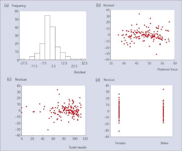

  

  Diagrams, using model residuals, for assessing the underlying assumptions in the multiple regression analysis

• The residuals have constant variability for all the fitted values of y. This is most easily verified by plotting the residuals against the predicted values of y; the resulting plot should produce a random scatter of points and should not exhibit any funnel effect (Fig. 2b).

• The relationship between y and each of the explanatory variables (there is only one χ in simple linear regression) is linear. This is most easily verified by plotting the residuals against the values of the explanatory variable; the resulting plot should produce a random scatter of points (Fig. 2c).

• The observations should be independent. This assumption is satisfied if each individual in the sample is represented only once (so that there is one point per individual in the scatter diagram in simple linear regression).

If all of the above assumptions are satisfied, the multiple regression equation can be investigated further. If there is concern about the assumptions, the most important of which are linearity and independence, a transformation can be taken of either y or of one or more of the χ's, or both, and a new multiple regression equation determined. The assumptions underlying this redefined model have to be verified before proceeding with the multiple regression analysis.

Example

A study assessed the impact of oral health on the life quality of patients attending a primary dental care practice, and identified the important predictors of their oral health related quality of life. The impact of oral health on life quality was assessed using the UK oral health related quality of life measure, obtained from a sixteen-item questionnaire covering aspects of physical, social and psychological health (McGrath et al., 2000).⁷ The data relate to a random sample of 161 patients selected from a multi-surgery NHS dental practice. Oral health quality of life score (OHQoL) was regressed on the explanatory variables shown in Table 2 (page 677) with their relevant codings ('tooth health' is a composite indicator of dental health generated from attributing weights to the status of the tooth: 0 = missing, 1 = decayed, 2 = filled and 4 = sound).

The output obtained from the analysis includes an analysis of variance table (Table 1, page 677). The F-ratio obtained from this table equals 5.68, with 9 degrees of freedom in the numerator and 151 degrees of freedom in the denominator. The associated P-value, P < 0.001, indicates that there is substantial evidence to reject the null hypothesis that all the partial regression coefficients are equal to zero. Additional information from the output gives an adjusted R²= 0.208, indicating that approximately one fifth of the variability of OHQoL is explained by its linear relationship with the explanatory variables included in the model. This implies that approximately 80% of the variation is unexplained by the model.

Incorporating the estimated regression coefficients from Table 2 into an equation, gives the following estimated multiple regression model: 

OHQoL = 52.58 – 2.83gender + 2.97age – 3.28socialclass – 5.60toothache – 2.53brokenteeth – 3.08baddenture – 1.79sore – 4.02looseteeth + 0.079toothhealth

The estimated coefficients of the model can be interpreted in the following fashion, using both a binary variable (gender) and a numerical variable (tooth health) as examples:

OHQoL is 2.8 less for males, on average, than it is for females (ie it decreases by 2.8 when gender increases by one unit, going from females to males), after adjusting for all the other explanatory variables in the model, and

OHQoL increases by 0.079 on average as the tooth health score increases by one unit, after adjusting for all the other explanatory variables in the model.

It can be seen from Table 2 that the coefficients that are significantly different from zero, and therefore judged to be important independent predictors of OHQoL, are gender (males having a lower mean OHQoL score than females), social class (those in higher social classes having a higher mean OHQoL score), tooth health (those with a higher tooth health score having a higher mean OHQoL score), and having a toothache in the last year (those with toothache having a lower mean OHQoL score than those with no toothache). Whether or not the patient was older or younger than 55 years, had or did not have a poor denture, sore gums or loose teeth in the last year were not significant (P > 0.05) independent predictors of OHQoL.

The four components, a,b,c and d, of Figure 2 are used to test the underlying assumptions of the model. In Figure 2a, it can be seen from the histogram of the residuals that their distribution is approximately Normal. When the residuals are plotted against the predicted (ie fitted) values of OHQoL (Fig. 2b), there is no tendency for the residuals to increase or decrease with increasing predicted values, indicating that the constant variance assumption is satisfied. It should be noted, furthermore, that the residuals are evenly scattered above and below zero, demonstrating that the mean of the residuals is zero. Figure 2c shows the residuals plotted against the numerical explanatory variable, tooth health. Since there is no systematic pattern for the residuals in this diagram, this suggests that the relationship between the two variables is linear. Finally, considering gender which is just one of the binary explanatory variables, it can be seen from Fig. 2d that the distribution of the residuals is fairly similar in males and females, suggesting that the model fits equally well in the two groups. In fact, similar patterns were seen for all the other explanatory variables, when the residuals were plotted against each of them. On the basis of these results, it can be concluded that the assumptions underlying the multiple regression analysis are satisfied.

A logistic regression analysis was also performed on this data set. The oral health quality of life score was scored as 'zero' in those individuals with values of less than or equal to 42 (the median value in a 1999 national survey), and as 'one' if their values were greater 42, the latter grouping comprising individuals believed to have an enhanced oral health related quality of life. The outcome variable in the logistic regression was then the logit of the proportion of individuals with an enhanced oral health quality of life; the explanatory variables were the same as those used in the multiple regression analysis. Having a toothache, a poorly fitting denture or loose teeth in the last year as well as being of a lower social class were the only variables which resulted in an odds ratio of enhanced oral health quality of life which was significantly less than one; no other coefficients in the model were significant. For example, the estimated coefficient in the logistic regression equation associated with toothache was –1.84 (P < 0.001); therefore, the estimated odds ratio for an enhanced oral health quality of life was its exponential equal to 0.16 (95% confidence interval 0.06 to 0.43). This suggests that the odds of an enhanced oral health quality of life was reduced by 84% in those suffering from a toothache in the last year compared with those not having a toothache, after taking all the other variables in the model into account.

It should be noted, however, that when the response variable is really quantitative, it is generally better to try to find an appropriate multiple regression equation rather than to dichotomise the values of y and fit a logistic regression model. The advantage of the logistic regression in this situation is that it may be easier to interpret the results of the analysis if the outcome can be considered a 'success' or a 'failure', but dichotomising the values of y will lose information; furthermore, the significance and values of the regression coefficients obtained from the logistic regression will depend on the arbitrarily chosen cut-off used to define 'success' and 'failure'.

References

Bulman JS Osborn JF Statistics in Dentistry. London: British Dental Journal Books 1989.
Chatterjee S Price B Regression Analysis by Example. 3rd edn Chichester: Wiley 1999.
Petrie A Sabin C Medical Statistics at a Glance. Oxford: Blackwell Science 2000.
Armitage P Berry G Matthews J NS Statistical Methods in Medical Research. 4th edn. Oxford: Blackwell Scientific Publications 2001.
Kleinbaum DG Klein M Logistic Regression: a Self-Learning Text. Heidelberg: Springer 2002.
Menard S Applied Logistic Regression Analysis. Sage University Paper series on Quantitative Applications in the Social Sciences, series no 07–106 Town: Sage University Press 1995.
McGrath C Bedi R Gilthorpe MS Oral health related quality of life – views of the public in the United Kingdom. Community Dent Health 2000; 17: 3–7.
Acknowledgements
The authors would like to thank Dr Colman McGrath for kindly providing the data for the example.
Author information
Authors and Affiliations
Corresponding author
Additional information
Refereed paper
Rights and permissions
About this article
Cite this article
Petrie, A., Bulman, J. & Osborn, J. Further statistics in dentistry Part 6: Multiple linear regression. Br Dent J 193, 675–682 (2002). https://doi.org/10.1038/sj.bdj.4801659
Published:
Issue Date:
DOI: https://doi.org/10.1038/sj.bdj.4801659
This article is cited by
-
Pre- and postoperative management techniques. Before and after. Part 1: medical morbidities
British Dental Journal (2015)
Congenital auditory meatal atresia: a numerical review
European Archives of Oto-Rhino-Laryngology (2009)
Problems of correlations between explanatory variables in multiple regression analyses in the dental literature
British Dental Journal (2005)