


1. Introduction
Heider (Reference Heider1946, Reference Heider1958) proposed that people feel social tension when there are inconsistencies between their relationships with others and the relationships those others have among themselves. This tension would arise, for instance, if an individual is friends with two people who are enemies with each other. He proposed that people are motivated to reduce this social tension by changing their relationships to achieve structural balance. This was formalized in graph theory, and hence in social networks, in the context of a triad in which links between individuals can take
 $\pm 1$
and a triad is considered to be balanced when the multiplication of the three links in the triad results in a positive number (Cartwright and Harary, Reference Cartwright and Harary1956). In another approach the definition of structural balance is relaxed, treating triads with three negative links as balanced. This definition is sometimes noted as a weak version of balance theory (Leskovec et al., Reference Leskovec, Huttenlocher and Kleinberg2010b).
$\pm 1$
and a triad is considered to be balanced when the multiplication of the three links in the triad results in a positive number (Cartwright and Harary, Reference Cartwright and Harary1956). In another approach the definition of structural balance is relaxed, treating triads with three negative links as balanced. This definition is sometimes noted as a weak version of balance theory (Leskovec et al., Reference Leskovec, Huttenlocher and Kleinberg2010b).
Models of structural balance show that networks tend to go to balanced states (Kułakowski et al., Reference Kułakowski, Gawroński and Gronek2005; Antal et al., Reference Antal, Krapivsky and Redner2005). But real-world networks that have been examined show features that are fundamentally at odds with structural balance (Leskovec et al., Reference Leskovec, Huttenlocher and Kleinberg2010b). One of the suggestions for why real-world networks do not tend to be in balanced states is because people do not make decisions about relationships merely based on the relationships they and others already have, but people also decide to have a relationship with someone based on attributes those individuals share (Doreian, Reference Doreian2002; Rivera et al., Reference Rivera, Soderstrom and Uzzi2010; Yap and Harrigan, Reference Yap and Harrigan2015; Bahulkar et al., Reference Bahulkar, Szymanski, Lizardo, Dong, Yang and Chawla2016).
Most of the literature interprets structural balance as an optimal state of a network because unbalanced structures are considered unstable (Marvel et al., Reference Marvel, Strogatz and Kleinberg2009; Singh et al., Reference Singh, Dasgupta and Sinha2014; Du et al., Reference Du, He and Feldman2016; Belaza et al., Reference Belaza, Hoefman, Ryckebusch, Bramson, Van Den Heuvel and Schoors2017; Saeedian et al., Reference Saeedian, Azimi-Tafreshi, Jafari and Kertesz2017; Rabbani et al., Reference Rabbani, Shirazi and Jafari2019; Pham et al., Reference Pham, Kondor, Hanel and Thurner2020, Reference Pham, Korbel, Hanel and Thurner2022; Malarz and Hołyst, Reference Malarz and Hołyst2022). But it is also possible to see balanced states as nonoptimal (Du et al., Reference Du, He, Wang and Feldman2018), especially when advantages for the society are considered. A network in structural balance will be composed of two groups [or more than two with the weak definition; Doreian (Reference Doreian2002); Davis (Reference Davis1967); Leskovec et al., (Reference Leskovec, Huttenlocher and Kleinberg2010b)], where all members of a group have positive relationships with all other members of that group and negative relationships with all members of the other group. Such structurally balanced groups, therefore, are perfectly polarized (Srinivasan, Reference Srinivasan2011). A different case of a balanced network is a system without negative connections. This state is called paradise (Antal et al., Reference Antal, Krapivsky and Redner2005; Krawczyk et al., Reference Krawczyk, Kaluzny and Kułakowski2017).
The establishment of these antagonistic groups in models of Kułakowski et al. (Reference Kułakowski, Gawroński and Gronek2005) and Antal et al. (Reference Antal, Krapivsky and Redner2005) is completely arbitrary, based on the random link weights assigned initially. This can be seen as a type of unprincipled polarization: there is no intrinsic reason individuals should be in one group instead of another. Such a situation could occur when the network is mature, or when network affiliation is only based on claims of similarity—sometimes called “echo chambers” in social media (Baumann et al., Reference Baumann, Lorenz-Spreen, Sokolov and Starnini2020; Gajewski et al., Reference Gajewski, Sienkiewicz and Hołyst2022). All members of the echo chamber have similar opinions, which are additionally strengthened through mutual interactions. This can be a bad thing from the perspective of the larger group. If a large group, such as a society, is attempting to accomplish some goals, such as democratically electing representatives to solve problems facing the society, then the rise of arbitrary antagonistic groups within the larger group may prevent achieving those goals. Such a situation occurs in the case of a polarized political scene divided into two camps [e.g., in a two-party system; Altafini (Reference Altafini2012)]. See Du et al. (Reference Du, He, Wang and Feldman2018) for a thorough discussion of issues arising from polarization in this context.
Recent models have shown that incorporating binary attributes can destabilize networks that would otherwise reach structural balance, preventing polarization (Chen et al., Reference Chen, Chen, Sun, Zhang, Zhang and Li2014; Du et al., Reference Du, He and Feldman2016; He et al., Reference He, Du, Cai and Feldman2018; Du et al., Reference Du, He, Wang and Feldman2018; Pham et al., Reference Pham, Kondor, Hanel and Thurner2020). Even a small number of binary attributes can disrupt structural balance/polarization (Górski et al., Reference Górski, Bochenina, Hołyst and D’Souza2020). Other models that considered continuous attributes, however, show that incorporating attributes may make structural balance an even more likely outcome (Flache and Macy, Reference Flache and Macy2011; Parravano et al., Reference Parravano, Andina-Díaz and Meléndez-Jiménez2016; Agbanusi and Bronski, Reference Agbanusi and Bronski2018; Gao and Wang, Reference Gao and Wang2018; Gao et al., Reference Gao, Wang, Zhang, Huang and Wang2018; Schweighofer et al., Reference Schweighofer, Garcia and Schweitzer2020a, Reference Schweighofer, Schweitzer and Garcia2020b). Previous work on the effect of attributes on polarization has been piecemeal, with no general framework for considering the effect of different types of attributes, which could account for the apparent inconsistencies when considering binary compared to continuous attributes.
Measures of polarization proposed in the literature depend on the system that is being investigated (Interian et al., Reference Interian, Marzo, Mendoza and Ribeiro2023). Most analyses focus on political parties and parliaments. In such cases, polarization can be measured either at the party level or at the level of MPs. In the former, polarization is defined using information about party ideologies and party sizes (Maoz and Somer-Topcu, Reference Maoz and Somer-Topcu2010; Sørensen, Reference Sørensen2014). In the latter, voting data (Neal, Reference Neal2020) (or other data related to MP’s actions) is used to obtain similarities between politicians, and polarization is usually associated with observed modularity (Porter et al., Reference Porter, Mucha, Newman and Warmbrand2005; Moody and Mucha, Reference Moody and Mucha2013). In terms of other systems, there are a large number of papers studying the polarization of opinions, e.g. Gajewski et al. (Reference Gajewski, Sienkiewicz and Hołyst2022); Schweighofer et al. (Reference Schweighofer, Schweitzer and Garcia2020b). In those proposed agent-based models, opinions evolve either toward consensus or polarized states. Here, we are interested in identity polarization (Rawlings, Reference Rawlings2022) defined as individuals having positive and negative interactions toward in-group and outgroup members, respectively (Xiao et al., Reference Xiao, Ordozgoiti and Gionis2020; Huang et al., Reference Huang, Silva and Singh2022). Polarization may be caused by simply disdaining the other side and not just by having a disagreement about policies (Mason, Reference Mason2018) thus we measure polarization using the relationships between people. Attributes affect those relations but also other processes (like structural balance) are in play.
The goal of this paper is to present a general framework to analyze the effect of attributes on signs in a network, specifically with an aim toward preventing or disrupting polarization. We study polarization and counteracting it in small- or medium-sized communities which are groups consisting of people that work together to achieve a common goal (e.g., business teams) or just co-exist (e.g., a class of students, a local community of residents). In those scenarios, polarization may appear, hampering the group’s performance or leading to negative effects, such as antipathy or bullying behaviors. We present an analytical framework for analyzing the impact of attributes on polarization. Considered attributes are those that change much more slowly than do relationships—which may include people’s immutable characteristics (e.g., race, sex), approximately immutable characteristics (e.g., wealth, religion, hobbies), and even characteristics that are thought to change relatively rapidly though more slowly than newly forming relationships (e.g., political opinions, etc.). Any attribute that can be described in a mathematical way as a differential change in likelihood of forming a positive relationship with people who share or differ on the attribute and for which an expected value can be found can be analyzed for its ability to destabilize a polarized system. Destabilization is more amenable to analytical approaches because the effect of an attribute can be linearized around the stable point. For the prevention of polarization and the analysis of attributes for which an expected value cannot be found, we present a numerical simulation framework that allows us to examine them. We then use the structure of real-world networks to look at how the relaxation of some assumptions of our model and the incorporation of attribute dynamics may alter the ties on those networks. From this we can draw interesting conclusions about how efforts to depolarize a polarized community may impact local communities. We do not claim to have detailed all possible attribute types—the ones we give serve to highlight the approach—and the code referenced at the end of this paper can easily be adapted to include any type of attribute one can think of. We do not claim a comprehensive treatment of the problem of how attributes impact relationships in networks, but we present a framework that researchers, policymakers, and managers can use to analyze attributes and make decisions about how to use attributes to prevent or destabilize polarization in networks.
2. General framework
2.1 The general model
We assume a model of
 $N$
agents with an underlying network structure. Connected pairs of agents know each other, so form a relationship. We describe this relationship with a real-valued weight
$N$
agents with an underlying network structure. Connected pairs of agents know each other, so form a relationship. We describe this relationship with a real-valued weight
 $x_{ij}(t)$
given in range
$x_{ij}(t)$
given in range
 $[-1,1]$
. The sign of the weight signifies a friendly (+) or hostile (–) relation. This setup resembles the small- and medium-sized communities that characterize much of our modern interactions, and the vast majority of interactions throughout human history.
$[-1,1]$
. The sign of the weight signifies a friendly (+) or hostile (–) relation. This setup resembles the small- and medium-sized communities that characterize much of our modern interactions, and the vast majority of interactions throughout human history.
Moreover, each agent possesses a set of
 $G$
attributes, which are aspects of the agent that change on a much longer timescale than their relationships (their immutable, or approximately so, opinions, characteristics, features, etc.). Let us introduce the following notation:
$G$
attributes, which are aspects of the agent that change on a much longer timescale than their relationships (their immutable, or approximately so, opinions, characteristics, features, etc.). Let us introduce the following notation:
 $\mathbf{A}$
is a matrix of size
$\mathbf{A}$
is a matrix of size
 $N$
x
$N$
x
 $G$
of all agents’ attributes,
$G$
of all agents’ attributes,
 $\mathbf{A}_i$
is a vector of attributes of agent
$\mathbf{A}_i$
is a vector of attributes of agent
 $i$
, and
$i$
, and
 $A_i^g$
is the
$A_i^g$
is the
 $g$
-th attribute of agent
$g$
-th attribute of agent
 $i$
. These are the characteristics that can drive apart or bring together two agents.
$i$
. These are the characteristics that can drive apart or bring together two agents.
Here, we present a general framework to examine the effect of attributes on polarization that models the change in the relationships (link weights) between individuals. This is presented in Equation (1) as a differential equation that changes in time:
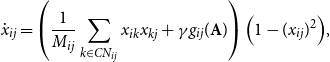 \begin{equation} \dot{x} _{ij} = \left (\frac{1}{M_{ij}} \sum _{k \in CN_{ij} } x_{ik} x_{kj} + \gamma g_{ij} (\mathbf{A}) \right ) \Big (1- (x_{ij}) ^ 2 \Big ), \end{equation}
where
 $CN_{ij}$
is the set of common neighbors of agents
$CN_{ij}$
is the set of common neighbors of agents
 $i$
and
$i$
and
 $j$
and
$j$
and
 $M_{ij}$
is the number of such agents. Let us also note that if agents
$M_{ij}$
is the number of such agents. Let us also note that if agents
 $i$
and
$i$
and
 $j$
do not have a relation, then
$j$
do not have a relation, then
 $x_{ij}$
does not exist and is not changed.
$x_{ij}$
does not exist and is not changed.
The right-hand side of Equation (1) is composed of three main parts: the two terms of the left factor and the right factor. On the left, we have the contribution of current relationships to relationships in the next time step. Sum elements
 $x_{ik} x_{kj}$
lead the network to follow the principles of structural balance theory. For instance, if pairs of agents
$x_{ik} x_{kj}$
lead the network to follow the principles of structural balance theory. For instance, if pairs of agents
 $i,k$
and
$i,k$
and
 $j,k$
are enemies, then the product
$j,k$
are enemies, then the product
 $x_{ik} x_{kj}$
is positive moving the relationship
$x_{ik} x_{kj}$
is positive moving the relationship
 $x_{ij}$
toward friendship. This is in agreement with the “enemy of my enemy is my friend” principle. If this is the only term in the left factor, the model will lead to paradise (everyone gets along with everyone else) or polarization in the form of (approximately) strong structural balance (Kułakowski et al., Reference Kułakowski, Gawroński and Gronek2005; Marvel et al., Reference Marvel, Kleinberg, Kleinberg and Strogatz2011).
$x_{ij}$
toward friendship. This is in agreement with the “enemy of my enemy is my friend” principle. If this is the only term in the left factor, the model will lead to paradise (everyone gets along with everyone else) or polarization in the form of (approximately) strong structural balance (Kułakowski et al., Reference Kułakowski, Gawroński and Gronek2005; Marvel et al., Reference Marvel, Kleinberg, Kleinberg and Strogatz2011).
The second part consists of
 $\gamma$
and
$\gamma$
and
 $g_{ij}(\mathbf{A})$
.
$g_{ij}(\mathbf{A})$
.
 $g_{ij} (\mathbf{A})$
is a function (more thoroughly described in Section 4.2) that relates the similarity between the attributes of two individuals to their relationship. The sign of
$g_{ij} (\mathbf{A})$
is a function (more thoroughly described in Section 4.2) that relates the similarity between the attributes of two individuals to their relationship. The sign of
 $\gamma g_{ij} (\mathbf{A})$
corresponds to the positive or negative effect of similarity between attributes on the relationship between agents. Extensive work has shown that there are some traits for which similar individuals have more chances for positive interactions—homophily (Mcpherson et al., Reference Mcpherson, Smith-lovin and Cook2001). Alternatively, the sign of this term may arise through a process such as the repulsion hypothesis, where individuals who are different from one another tend to dislike each other (Rosenbaum, Reference Rosenbaum1986). The parameter
$\gamma g_{ij} (\mathbf{A})$
corresponds to the positive or negative effect of similarity between attributes on the relationship between agents. Extensive work has shown that there are some traits for which similar individuals have more chances for positive interactions—homophily (Mcpherson et al., Reference Mcpherson, Smith-lovin and Cook2001). Alternatively, the sign of this term may arise through a process such as the repulsion hypothesis, where individuals who are different from one another tend to dislike each other (Rosenbaum, Reference Rosenbaum1986). The parameter
 $\gamma$
corresponds to the relative strength of considered attributes compared to the drive toward structural balance. If
$\gamma$
corresponds to the relative strength of considered attributes compared to the drive toward structural balance. If
 $\gamma =0$
, then only the triadic balance matters. If
$\gamma =0$
, then only the triadic balance matters. If
 $\gamma \gg 1$
, then the attribute (dis)similarity is of significance. The last term in Equation (1), that is, the second factor, is a normalization term that limits the relationship values to their domain
$\gamma \gg 1$
, then the attribute (dis)similarity is of significance. The last term in Equation (1), that is, the second factor, is a normalization term that limits the relationship values to their domain
 $[-1,+1]$
.
$[-1,+1]$
.
In effect, each pair of agents can be described by two types of connections: a link related to the relationship (one is more likely to develop a positive relationship with someone who shares similar positive and negative relationships) and a link related to the similarity of attributes (one is more likely to develop a positive relationship with someone with whom they share attributes in common). Thus, the structure of the network is a multiplex (Kivelä et al., Reference Kivelä, Arenas, Barthelemy, Gleeson, Moreno and Porter2014) with two layers: the relation layer with weights
 $x_{ij}(t)$
and the attribute layer with weights
$x_{ij}(t)$
and the attribute layer with weights
 $g_{ij} (\mathbf{A})$
. The diagram of interactions in the model is presented in Figure 1. Importantly, the interlayer links connect not the corresponding agents but the corresponding links. Such a structure is called a link multiplex (Górski et al., Reference Górski, Kułakowski, Gawroński and Hołyst2017).
$g_{ij} (\mathbf{A})$
. The diagram of interactions in the model is presented in Figure 1. Importantly, the interlayer links connect not the corresponding agents but the corresponding links. Such a structure is called a link multiplex (Górski et al., Reference Górski, Kułakowski, Gawroński and Hołyst2017).
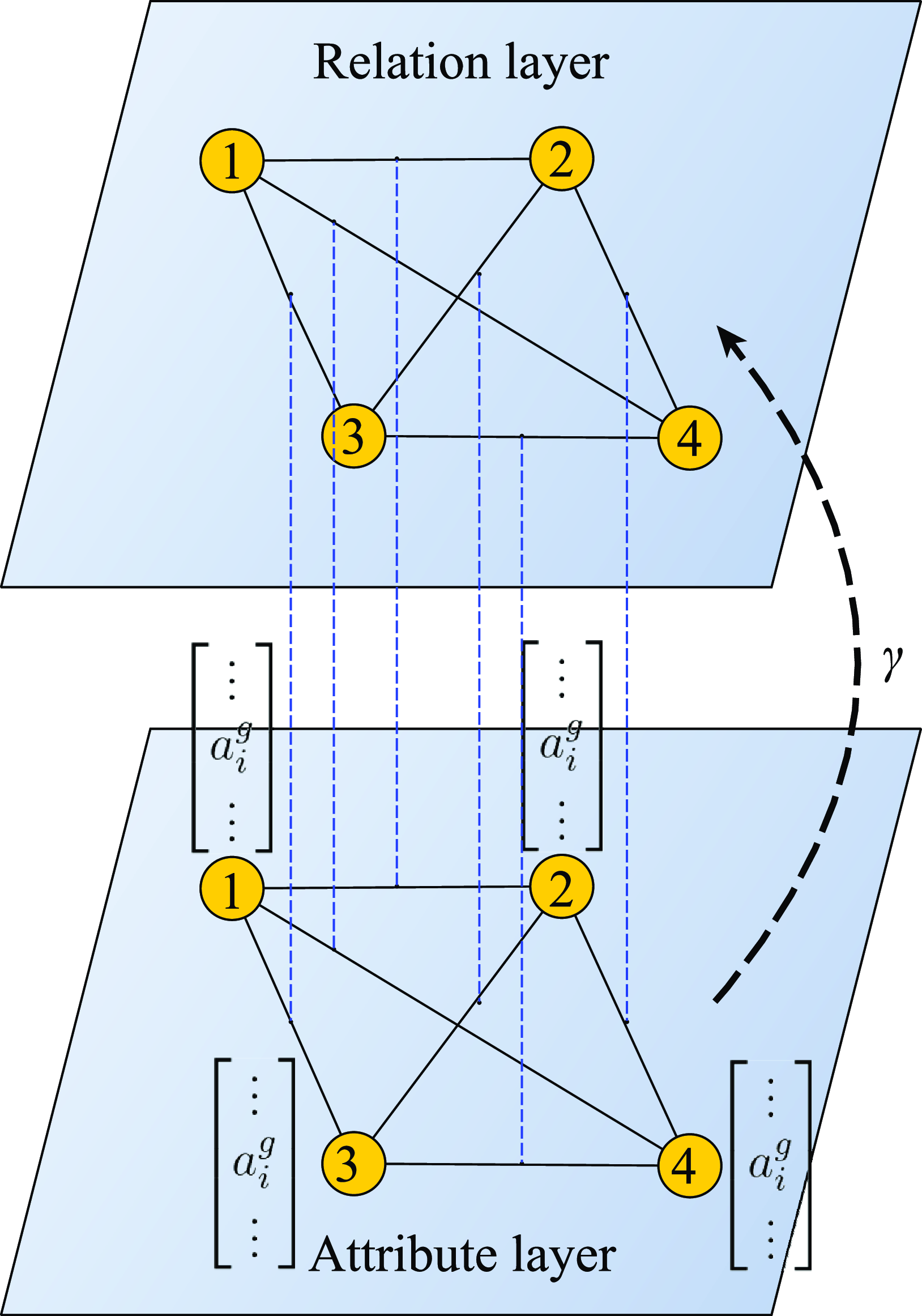
Figure 1. A diagram shows how the attribute layer affects the relationship layer. The structure of such a system is a link multiplex. Each agent has a
 $\{a_i^g\}$
attribute set that allows us to specify the weights of
$\{a_i^g\}$
attribute set that allows us to specify the weights of
 $ g_{ij}$
in the attribute layer. The measure of the impact of one layer on another is the
$ g_{ij}$
in the attribute layer. The measure of the impact of one layer on another is the
 $ \gamma$
coefficient. In the adopted model, the weights
$ \gamma$
coefficient. In the adopted model, the weights
 $ x_{ij}$
of the relation layers do not affect the attribute layer. In the figure, only one edge is labeled on each layer.
$ x_{ij}$
of the relation layers do not affect the attribute layer. In the figure, only one edge is labeled on each layer.
When allowing the system to evolve, it will finally reach one of the stable points. In the stable point, all or almost all relations become
 $x_{ij}=\pm 1$
. This always happens except when the first factor of Equation (1) is 0, see section 4 in Supplementary Material (SM) for more details. Analysis of the final state that was reached is performed in order to examine the effect of attributes on polarization.
$x_{ij}=\pm 1$
. This always happens except when the first factor of Equation (1) is 0, see section 4 in Supplementary Material (SM) for more details. Analysis of the final state that was reached is performed in order to examine the effect of attributes on polarization.
2.2 Attribute schema
We propose a nonexhaustive schema (partially inspired by Gower, Reference Gower1971) for types of attributes that relies on three parameters (Figure 2). As our attribute layer does not evolve, these attributes are best described as traits that change on a much longer timescale than relationships. This clearly includes some things that are typically thought of as opinions (e.g., political party preferences) and excludes some (e.g., whether sanctions are an effective deterrent). Furthermore, this makes the question of whether or not any given trait of a person could be conceptualized as an attribute in this framework an empirical question: does the value for this trait for the average individual in the system change at a much slower rate than the average strength of relationship changes? From the perspective of the relationship strengths, these attributes can be thought of as (relatively) immutable characteristics of a person.

Figure 2. Classification of considered types of attributes. In the first split we consider ordered and unordered attributes for which different categories can or cannot be arranged on the axis, respectively. Each attribute has
 $v$
categories. An additional parameter
$v$
categories. An additional parameter
 $\alpha$
for unordered attributes differentiates attribute types by how much having different categories negatively affects the relation. With
$\alpha$
for unordered attributes differentiates attribute types by how much having different categories negatively affects the relation. With
 $\alpha =1$
we have negative unordered attributes for which positive and negative magnitudes of the impact of the same and different attributes are equal. When
$\alpha =1$
we have negative unordered attributes for which positive and negative magnitudes of the impact of the same and different attributes are equal. When
 $v=2$
, ordered attributes and negative unordered attributes are indistinguishable and are called binary attributes. Thick borders surround five classes of attributes that were analyzed in detail.
$v=2$
, ordered attributes and negative unordered attributes are indistinguishable and are called binary attributes. Thick borders surround five classes of attributes that were analyzed in detail.
Things defined as attributes in this way can be placed in a taxonomy based on how they impact the relationships of individuals who share or differ on the attribute. First, we can divide attributes into ordered and unordered attributes. Ordered attributes (OAs) are those for which how close another person’s attributes are to your own influences how much the attributes affect the sign of a link. An example of an ordered attribute is the number of children someone has. Unordered attributes (UAs) are those where there is no natural ordering of categories, including attributes such as race, (possibly) political affiliation, language, etc. Within both of the classes of attributes, you can adjust how many categories there are (given as
 $v$
in Figure 2). If there are only two categories, this is a binary attribute (BA; many of these attributes may be things that put a person in opposition to others—e.g., whether someone lives in the same or a different city than me or supporting Manchester City or Manchester United when living in Manchester). If there are infinitely many categories for an ordered attribute, this is a continuous attribute (CA e.g., income). Infinitely many categories for an unordered attribute would treat every individual as unique, so we do not consider them here.
$v$
in Figure 2). If there are only two categories, this is a binary attribute (BA; many of these attributes may be things that put a person in opposition to others—e.g., whether someone lives in the same or a different city than me or supporting Manchester City or Manchester United when living in Manchester). If there are infinitely many categories for an ordered attribute, this is a continuous attribute (CA e.g., income). Infinitely many categories for an unordered attribute would treat every individual as unique, so we do not consider them here.
Ordered attributes follow both homophily and repulsion theories, that is, there is a tendency for people to form (un)friendly relations with (dis)similar others. Within the class of unordered attributes, we can consider whether individuals are drawn toward others in their same category and/or pushed away from members in other categories. Thus, UAs also comply with the homophily theory but we distinguish negative unordered attributes (NUAs) (e.g., religion, political affiliation, which football club one supports) and positive unordered attributes (PUAs) (e.g., whether one plays chess or enjoys fishing) as such that follow or not repulsion theory, respectively. For example, liking fishing may only cause similar people to have more positive interactions but not cause dissimilar people to have more negative interactions (i.e., one does not typically dislike someone for how much they like fishing). On the other hand, an attribute such as political affiliation may lead to an increase in the negative relationship with members in other categories than one’s own similarly to the increase in positive relationship with members in one’s own category. From the mathematical point of view, let us denote the ratio of strength of negative feelings toward members of other categories to strength of positive feelings to members of one’s own category as
 $\alpha$
(see Methods for mathematical details). Therefore, for
$\alpha$
(see Methods for mathematical details). Therefore, for
 $\alpha =0$
we obtain a positive unordered attribute with no negative influence and
$\alpha =0$
we obtain a positive unordered attribute with no negative influence and
 $\alpha =1$
gives a negative unordered attribute with equal negative and positive influence.
$\alpha =1$
gives a negative unordered attribute with equal negative and positive influence.
3. Research questions
We are interested in the effect of attributes on two parts of the network formation process: (A) how attributes can destabilize a polarized network and (B) how attributes can prevent a polarized network from forming. This leads to a set of research questions and specific methods to address them.
A. How can a polarized state be destabilized? Let us imagine that a certain group (e.g., a class of students) became divided. The reason why polarization appeared is irrelevant here. The aim of the attributes would be to change the situation. Having a polarized state initially, it is feasible to perform linearization of the effects of attributes on the relation layer. This allows us to make claims about attributes in general. This analytical reasoning can be confirmed using simulations. Numerical simulations are also used to draw conclusions about specific attribute types.
B. How can polarization be prevented? It could be the case that a social network is formed anew, and preventing polarization could be a main initial goal. This could occur when new working groups are formed in a company, for example. Addressing this question largely requires the use of numerical simulations.
To investigate these issues, we will examine how the types of attributes and their associated parameters differently impact destabilization and prevention of polarization. This will lead to us investigating the number of attributes (
 $G$
), the strength of the attribute layer (
$G$
), the strength of the attribute layer (
 $\gamma$
), the number of categories in the attribute (
$\gamma$
), the number of categories in the attribute (
 $v$
) and the number of agents in the system (
$v$
) and the number of agents in the system (
 $N$
).
$N$
).
4. Methods
In this section, we first describe the network structures that will be further used to test the model. Then, we discuss how we obtain the similarity
 $ g_{ij}$
based on the attribute matrix
$ g_{ij}$
based on the attribute matrix
 $\mathbf{A}$
. The Section 4.3 describes how to determine the polarization of a system. At the end of this methodology, we explain the details of the numerical simulations.
$\mathbf{A}$
. The Section 4.3 describes how to determine the polarization of a system. At the end of this methodology, we explain the details of the numerical simulations.
4.1 Considered network structures
To test our model in various settings, we employed four different network topologies: a complete graph and three network structures that are based on real data. A complete graph is a topology simulating a situation where relations exist between all pairs of agents. It is in most cases an unrealistic scenario. However, it is a valid approximation of a small community where everybody knows each other. Such an approach is also often used for relatively large communities (Górski et al., Reference Górski, Bochenina, Hołyst and D’Souza2020) to facilitate analytical computations and because it allows one to observe the effects of dynamics abstracting away from the topology. Similarly, our analytics shown in Section 5.1 are based on complete graphs. However, further numerical results let us extend the obtained conclusions for other network structures.
For a complete graph, each pair of agents has
 $M_{ij}=N-2$
common neighbors and the Equation (1) becomes
$M_{ij}=N-2$
common neighbors and the Equation (1) becomes
 \begin{equation} \dot{x} _{ij} = \left (\frac{1}{N-2} \sum _{k = 1 } ^{N} x_{ik} x_{kj} + \gamma g_{ij} (\mathbf{A}) \right ) \Big (1- (x_{ij}) ^ 2 \Big ) . \end{equation}
Following Andres et al. (Reference Andres, Casiraghi, Vaccario and Schweitzer2022), we considered three network structures based on real datasets. The details of the networks are presented in Table 1. Network visualizations are shown in Figure 2 in SM. From these datasets, we take realistic social structures of relations. As signs of edges are not given, we either infer the polarities from the known division into communities or assign them randomly in order to investigate destabilizing and preventing polarization scenarios (see also Section 4.4 for more details). Even if a dataset contains the numbers of contacts between agents, we did not use this information. This allows us to obtain more general results and not have results rely on the applied method of obtaining relation weights
 $x_{ij}$
from the given interactions’ intensities. The untested method could lead to incomplete or misleading conclusions. The first dataset consists of recorded face-to-face interactions in the period of 7 weekdays between high school students belonging to nine classes (Mastrandrea et al., Reference Mastrandrea, Fournet and Barrat2015). A class setting is a small community of which a complete network is a good approximate structure. Therefore, we extracted contact data related to one chosen class coded as 2BIO1. The second dataset is a well-known Zachary karate club (ZKC) network (Zachary, Reference Zachary1977). The network was obtained just before the club breakdown into two separate clubs following the conflict between the club president and one of the instructors. The third dataset comprises contacts in the windsurfers’ community (Freeman et al., Reference Freeman, Freeman and Michaelson1988). The network consists of two groups: old members and newcomers. No conflict was registered but it was observed that windsurfers preferred to spend time with the members of their group.
$x_{ij}$
from the given interactions’ intensities. The untested method could lead to incomplete or misleading conclusions. The first dataset consists of recorded face-to-face interactions in the period of 7 weekdays between high school students belonging to nine classes (Mastrandrea et al., Reference Mastrandrea, Fournet and Barrat2015). A class setting is a small community of which a complete network is a good approximate structure. Therefore, we extracted contact data related to one chosen class coded as 2BIO1. The second dataset is a well-known Zachary karate club (ZKC) network (Zachary, Reference Zachary1977). The network was obtained just before the club breakdown into two separate clubs following the conflict between the club president and one of the instructors. The third dataset comprises contacts in the windsurfers’ community (Freeman et al., Reference Freeman, Freeman and Michaelson1988). The network consists of two groups: old members and newcomers. No conflict was registered but it was observed that windsurfers preferred to spend time with the members of their group.
Table 1. Description of considered datasets
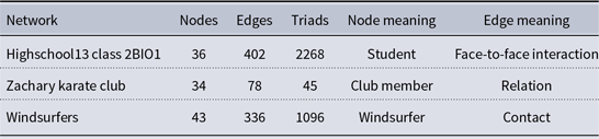
References and a longer description are given in the text.
The chosen set of real network structures allows us to test our simulation assumptions and consider the effect of attributes on polarization in more realistic situations. First, the most detailed simulations were performed for complete graphs and Highschool dataset allows us to check whether similar results are also obtained when not all relations exist. Moreover, this network contains only a single community, thus there are not any reasons for assigning particular signs of relations to agents. Therefore, this dataset is also a good structure for testing scenario B (i.e., preventing polarization from forming). Of course, the destabilization scenario may also be analyzed. Second, trying to destabilize a system is particularly interesting in the case of networks where separate groups can be distinguished. This is the case for ZKC and Windsurfers datasets. For these networks, one can test the destabilization scenario assuming that agents belonging to the same group have positive relations and agents belonging to different groups are connected via negative links.
4.2 Attributes, distances and similarity between agents
In general, the weight in the attribute layer between agent
 $ i$
and agent
$ i$
and agent
 $ j$
is a function that depends on the attributes of all agents:
$ j$
is a function that depends on the attributes of all agents:
 $g_{ij}(\mathbf{A})$
. However, we make several assumptions that make approximations possible:
$g_{ij}(\mathbf{A})$
. However, we make several assumptions that make approximations possible:
-
No direct influence of node
 $ k$
’s attributes on the similarity
$ g_{ij}$
if
$k\neq i$
and
$k\neq j$
. Thus,(3)where
\begin{equation} g_{ij} (\mathbf{A}) = g_{ij} \left(\mathbf{A} _i, \mathbf{A} _j\right), \end{equation}
$\mathbf{A}_i=\left[a_i^1,\ldots,a_i^G\right]$
. This approximation treats all nodes homogeneously, as compared to the opposite scenario where attributes of some agents play a significant role (Kacperski and Hołyst, Reference Kacperski and Hołyst1999; Hołyst et al., Reference Hołyst, Kacperski and Schweitzer2000). In the real world, this assumption signifies that there are no, for example, leaders in the network.
$ k$
’s attributes on the similarity
$ g_{ij}$
if
$k\neq i$
and
$k\neq j$
. Thus,(3)where
\begin{equation} g_{ij} (\mathbf{A}) = g_{ij} \left(\mathbf{A} _i, \mathbf{A} _j\right), \end{equation}
$\mathbf{A}_i=\left[a_i^1,\ldots,a_i^G\right]$
. This approximation treats all nodes homogeneously, as compared to the opposite scenario where attributes of some agents play a significant role (Kacperski and Hołyst, Reference Kacperski and Hołyst1999; Hołyst et al., Reference Hołyst, Kacperski and Schweitzer2000). In the real world, this assumption signifies that there are no, for example, leaders in the network.
-
No correlations between the attributes, so that they are independent. Attributes are clearly not independent in the real world (e.g., hunting and baseball co-occur at higher than expected rates), but this does not violate that assumption. Specifically, it would be possible to do something like a principle components analysis on those traits and extract a smaller number of orthogonal (i.e., independent) dimensions. This assumption leads to weighted average across attributes:
(4)where a function
\begin{equation} g_{ij} (\mathbf{A} _i, \mathbf{A} _j) \equiv g_{ij} \Big (\left(a_i ^ 1, a_j^1\right), \ldots, \left(a_i ^ G, a_j ^ G\right) \Big ) = \dfrac{1}{\sum _g C_g} \sum _g C_g h_{ij} \left(a_i ^ g, a_j ^ g\right), \end{equation}
$ h_{ij}$
defines the similarity between individual attributes and
$ C_g$
is a constant related to the strength of the attribute
$g$
. For all types considered, it is assumed that
$ h_{ij} \big(a_i ^ g, a_j ^ g\big)$
is maximal when
$ a_i ^ g = a_j ^ g$
. Assuming attribute homogeneity (
$C_g=1$
), we obtain a simple average. The consequences of this assumption is that only those attributes that have the same relative impact on relationships should be included jointly in the analysis. It would, therefore, be possible to break a set of real-world attributes into such groups and analyze them as such. This assumption could be relaxed in the specific case we know that one attribute is more important than another (e.g., political affiliation is more important than liking baseball), then one can use varying strengths
$C_g$
.
-
Specifying the maximum (minimum) similarity value:
$ | h_{ij} | \le 1$
, which leads to
$ | g_{ij} | \le 1$
.


The above approximations lead to a measure related to the Gower similarity coefficient (Gower, Reference Gower1971). Importantly, the resultant matrices are amenable to statistical analysis. The approximations also mean that the attributes are independent, and the similarity between the set of attributes is the average of the similarities between the individual attributes. In our analysis, we assume that each agent has
 $ G$
attributes of the same type in a given simulation. The form of the
$ G$
attributes of the same type in a given simulation. The form of the
 $ h_{ij}$
function depends on the given type of attribute. Each attribute type has a certain set of permissible values (the so-called categories)
$ h_{ij}$
function depends on the given type of attribute. Each attribute type has a certain set of permissible values (the so-called categories)
 $\Omega _A$
, that is,
$\Omega _A$
, that is,
 $a_i^g \in \Omega _A$
. The
$a_i^g \in \Omega _A$
. The
 ${v} \equiv | \Omega _A |$
parameter specifies the number of allowed, different categories, so that
${v} \equiv | \Omega _A |$
parameter specifies the number of allowed, different categories, so that
 $\Omega _A = \{0,1, \ldots, v-1 \}$
.
$\Omega _A = \{0,1, \ldots, v-1 \}$
.
The following similarity function describes binary attributes (which are, equivalently, ordered or unordered attributes with two categories, i.e.,
 $v=2$
):
$v=2$
):
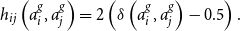 \begin{equation} h_{ij} \left(a_i ^ g, a_j ^ g\right) = 2 \left(\delta \left(a_i ^ g, a_j ^ g\right) -0.5 \right ). \end{equation}
The similarity function was selected to meet the conditions mentioned above. For the same value for the attribute, it takes the value of
 $ + 1$
, and for different values,
$ + 1$
, and for different values,
 $ -1$
.
$ -1$
.
The similarity function for ordered attributes is as follows [a different form can be found in Schweighofer et al. (Reference Schweighofer, Schweitzer and Garcia2020b)]:
 \begin{equation} h_{ij} \left(a_i ^ g, a_j ^ g\right) = 2 \left (0.5- \dfrac{\Big| a_i ^ g-a_j ^ g \big|}{v- 1} \right ) . \end{equation}
What differentiates ordered from unordered attributes is the existence of a majority/minority relationship between categories, for instance category 3 is closer to category 2 than it is to category 1 while category 2 is equally close to categories 1 and 3.
Unordered attributes can be generalized into categorical attributes with an additional
 $ \alpha$
parameter. This parameter denotes relative strength of attribute influence on relations when the attribute values are different as compared to the case when the attribute values are the same, that is,
$ \alpha$
parameter. This parameter denotes relative strength of attribute influence on relations when the attribute values are different as compared to the case when the attribute values are the same, that is,
 $ \big| h_{ij} \big(a_i ^ g \neq a_j ^ g\big) \big| = \alpha \big| h_{ij} \big(a_i ^ g = a_j ^ g\big) \big|$
. Here, we do not examine many possible values of
$ \big| h_{ij} \big(a_i ^ g \neq a_j ^ g\big) \big| = \alpha \big| h_{ij} \big(a_i ^ g = a_j ^ g\big) \big|$
. Here, we do not examine many possible values of
 $\alpha$
but we limit our analysis to two extreme cases. Negative unordered attributes are attributes whose similarity function is also given by Equation (5) with any number of possible values (
$\alpha$
but we limit our analysis to two extreme cases. Negative unordered attributes are attributes whose similarity function is also given by Equation (5) with any number of possible values (
 $ v \ge 2$
). The key for negative unordered attributes is that having different values on the attributes negatively impacts the relationship between agents, and this influence is as strong (in an absolute sense) as the effect of agents sharing a value for the attribute, that is,
$ v \ge 2$
). The key for negative unordered attributes is that having different values on the attributes negatively impacts the relationship between agents, and this influence is as strong (in an absolute sense) as the effect of agents sharing a value for the attribute, that is,
 $\alpha =1$
and
$\alpha =1$
and
 $ \big| h_{ij} \big(a_i ^ g = a_j ^ g\big) \big| = \big| h_{ij} \big(a_i ^ g \neq a_j ^ g\big) \big|$
. Another special case is when there is no effect of having different values for an attribute (i.e.,
$ \big| h_{ij} \big(a_i ^ g = a_j ^ g\big) \big| = \big| h_{ij} \big(a_i ^ g \neq a_j ^ g\big) \big|$
. Another special case is when there is no effect of having different values for an attribute (i.e.,
 $\alpha =0$
). We call these positive unordered attributes. They are described by the following similarity function:
$\alpha =0$
). We call these positive unordered attributes. They are described by the following similarity function:
 \begin{equation} h_{ij} \left(a_i ^ g, a_j ^ g\right) = \delta \left(a_i ^ g, a_j ^ g\right). \end{equation}
4.3 Measures of polarization
A single numerical simulation, described further in the next section, for specified coupling
 $\gamma$
consists of choosing initial values of relations, choosing the attribute values, and allowing the system to evolve according to Equations (1–2) until the stable point is reached. Such a stable point is the final state of the system and this state is used to evaluate the influence of attributes. We identify a triad as having 0, 1, 2, or 3 negative links by taking the signs of its relations in the final state
$\gamma$
consists of choosing initial values of relations, choosing the attribute values, and allowing the system to evolve according to Equations (1–2) until the stable point is reached. Such a stable point is the final state of the system and this state is used to evaluate the influence of attributes. We identify a triad as having 0, 1, 2, or 3 negative links by taking the signs of its relations in the final state
 $\mathrm{sgn}(x_{ij})$
.
$\mathrm{sgn}(x_{ij})$
.
As it was described in the Introduction, a polarized state (i.e., a state with mutually hostile groups) is a balanced state. The reverse statement is not true. A balanced state is not always a polarized one because a paradise state (which is balanced) is not considered polarized. Moreover, from a societal point of view an unbalanced state with all links negative (i.e., a “hell” state) is not advantageous. Therefore, taking into account the above notions and in order to determine the effect of attributes on reaching a polarized state, we introduce the following two measures of polarization:
-
Global polarization: A system is globally polarized when it is weakly balanced but not in a paradise state. In other words, when a system can be split into
$ K\gt$
1 antagonistic, nonempty groups, it is considered polarized. -
Local polarization: A triad is polarized when it has two or three negative links, because in such triads two or three hostile groups can be distinguished, respectively. The structurally unbalanced triad with one negative link is not polarized because a mediator-agent (Doreian and Mrvar, Reference Doreian and Mrvar2009) mediates between the enemy agents. Thus, the measure of local polarization
$P_{LP}$
in the whole system is the sum of the densities of the triangles with two (
$n_2$
) or three (
$n_3$
) negative links.(8)
\begin{equation} P_{LP} = n_2 + n_3 \end{equation}


Summing up, due to the fact that we consider a paradise state as nonpolarized and a triad with three negative links as polarized, our measures differ from the standard degree of structural balance (Aref and Wilson, Reference Aref and Wilson2018) which is the density of balanced triangles (i.e., without or with two negative links). This is also considered to be a measure of strong polarization by Neal (Reference Neal2020). In the system Neal studies, U.S. Congress, one can expect polarization to appear as a clear division between Democrats and Republicans, but in the general case, one cannot assume that, for instance, a paradise or a weakly balanced state is unlikely.
It is worth noting that for our measures, the necessary and sufficient condition for the state not to be globally polarized is that at least one triad with one negative link exists. In the analyses presented below, polarization is investigated only in the relation layer for the weights
 $ x_{ij}$
(not in the static attribute layer). Here we focus mostly on the local polarization results, because the necessary and sufficient condition means that the changes in global polarization probability are usually similar (see section 3 in SM for global polarization).
$ x_{ij}$
(not in the static attribute layer). Here we focus mostly on the local polarization results, because the necessary and sufficient condition means that the changes in global polarization probability are usually similar (see section 3 in SM for global polarization).
4.4 Details of the numerical simulations
We assume uniform distributions everywhere we draw random variables, that is: discrete, uniform distributions for attribute values in scenarios A and B and continuous uniform distributions for the relation layer weights in scenario B (
 $x_{ij}\in [-1,+1]$
). In scenario A, we divide agents into two hostile groups because it is assumed that the relation layer is initially very close to the balanced state [weights
$x_{ij}\in [-1,+1]$
). In scenario A, we divide agents into two hostile groups because it is assumed that the relation layer is initially very close to the balanced state [weights
 $ x_{ij}$
are set to
$ x_{ij}$
are set to
 $\pm 0.99$
and the product of weights
$\pm 0.99$
and the product of weights
 $ x_{ij} x_{jk} x_{ki}$
is positive in all triads (
$ x_{ij} x_{jk} x_{ki}$
is positive in all triads (
 $ ijk$
)]. This makes the relations follow in- and outgroup identifications and the obtained initial network is usually polarized. For complete graphs and for the high school dataset, agents are divided into the groups with equal probability, which makes the obtained results averaged over the group sizes and distributions. For ZKC and Windsurfers datasets, initial group participation was predefined.
$ ijk$
)]. This makes the relations follow in- and outgroup identifications and the obtained initial network is usually polarized. For complete graphs and for the high school dataset, agents are divided into the groups with equal probability, which makes the obtained results averaged over the group sizes and distributions. For ZKC and Windsurfers datasets, initial group participation was predefined.
In each simulation, agents only have attributes of the same type. Moreover, it is assumed that the significance of each attribute is the same:
 $ C_g =$
1 (this assumption is described above). The coupling strength
$ C_g =$
1 (this assumption is described above). The coupling strength
 $ \gamma$
can theoretically take any value. However, taking into account the theory of homophily, in further analyses, the strength of the attribute layer influence was limited to the nonnegative numbers
$ \gamma$
can theoretically take any value. However, taking into account the theory of homophily, in further analyses, the strength of the attribute layer influence was limited to the nonnegative numbers
 $ \gamma \ge 0$
. The obtained results for
$ \gamma \ge 0$
. The obtained results for
 $ \gamma \ge 0$
will allow straightforward model interpretation also for the negative influence
$ \gamma \ge 0$
will allow straightforward model interpretation also for the negative influence
 $ \gamma \lt 0$
.
$ \gamma \lt 0$
.
In the Results, analytical considerations and numerical results for the destabilization problem A and numerical results for problem B of inhibiting the appearance of a polarized state are presented. Each point in the plots was obtained due to averaging the results for at least 1000 different initial conditions. If given, error bars are standard deviations. The results for continuous attributes were obtained for ordered attributes with
 $v=1000$
. Figure 3 in SM shows this is a valid approximation.
$v=1000$
. Figure 3 in SM shows this is a valid approximation.
5. Results
5.1 Analytical results for destabilization
Because the network configuration is stable, we can linearize the differential equations and ask if stability is maintained in the face of small perturbations. We do this by analyzing the Jacobian matrix of this system of equations (see section 4.1 in SM for details). The conditions for destabilization of the link connecting the nodes
 $ i$
and
$ i$
and
 $ j$
are both the sign inequality of weights
$ j$
are both the sign inequality of weights
 $x_{ij}$
and
$x_{ij}$
and
 $g_{ij}$
, respectively, in the relation and attribute layers, and a greater influence of the attribute layer than of the edges in the relation layer:
$g_{ij}$
, respectively, in the relation and attribute layers, and a greater influence of the attribute layer than of the edges in the relation layer:
 \begin{align} \begin{cases} \text{sgn} (x_{ij}) \neq \text{sgn} (g_{ij}) \\| \gamma g_{ij} | \ge 1 \end{cases} \end{align}
A single destabilized edge in relation layer may induce further edge changes which may lead to a different but still polarized state. The sufficient condition for the end state of a single triad not to be polarized is that the similarities in the attribute layer form a triad with either 0 or 1 negative links and a sufficiently large value of the strength
 $ \gamma$
, so that the following inequalities are fulfilled for this triad:
$ \gamma$
, so that the following inequalities are fulfilled for this triad:
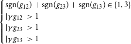 \begin{align} \begin{cases} \text{sgn}(g_{12}) + \text{sgn}(g_{23}) + \text{sgn}(g_{13}) \in \{1,3\} \\ | \gamma g_{12} |\gt 1 \\ | \gamma g_{23} |\gt 1 \\ | \gamma g_{13} |\gt 1 \end{cases} \end{align}
From the perspective of the measure of global polarization, the existence of at least one unbalanced triad with one negative link in attribute layer and a sufficiently large value of the strength
 $ \gamma$
is enough for the network not to be polarized. For local polarization, the more triads that fulfill Equation (10) there are, the larger decrease of polarization is expected.
$ \gamma$
is enough for the network not to be polarized. For local polarization, the more triads that fulfill Equation (10) there are, the larger decrease of polarization is expected.
Adopting a specific type of attribute enables a statistical analysis of its properties, allowing the approximate probability of meeting these conditions to be determined. In order to accurately analyze destabilization, numerical simulations are necessary to test whether the destabilization of a certain number of links will lead to an unpolarized state.
5.2 Statistical analysis of attributes in the context of destabilization
Now we are interested in asking which types of attributes lead to a lower chance of polarization. To do this, we need the probability density function of each similarity measure
 $h_{ij}$
, which allows us to calculate the expected value
$h_{ij}$
, which allows us to calculate the expected value
 $ \mathrm{E[}{h}\mathrm{]}$
and the variance
$ \mathrm{E[}{h}\mathrm{]}$
and the variance
 $ \mathrm{Var[}{h}\mathrm{]}$
. For a small number of attributes, the destabilization phenomenon is strongly dependent on the distribution
$ \mathrm{Var[}{h}\mathrm{]}$
. For a small number of attributes, the destabilization phenomenon is strongly dependent on the distribution
 $ h_{ij}$
, but for larger
$ h_{ij}$
, but for larger
 $ G$
values, the probability distribution of
$ G$
values, the probability distribution of
 $ g_{ij}$
begins to resemble a normal distribution with the mean and variance of
$ g_{ij}$
begins to resemble a normal distribution with the mean and variance of
 $ \mathrm{E[}{h}\mathrm{]}$
and
$ \mathrm{E[}{h}\mathrm{]}$
and
 $ \dfrac{\mathrm{Var[}{h}\mathrm{]}}{G}$
, respectively. For the value of
$ \dfrac{\mathrm{Var[}{h}\mathrm{]}}{G}$
, respectively. For the value of
 $ G \ge 5$
for considered types of attributes, the distribution of
$ G \ge 5$
for considered types of attributes, the distribution of
 $ g_{ij}$
is unimodal, and then the following reasoning can be made.
$ g_{ij}$
is unimodal, and then the following reasoning can be made.
The destabilization will certainly not happen if
 $ | \gamma g_{ij} | \lt 1$
occurs for all edges (i.e.,
$ | \gamma g_{ij} | \lt 1$
occurs for all edges (i.e.,
 $ | \gamma | \lt | g_{ij} | ^{- 1}$
; the influence of the relation layer is stronger than the influence of the attribute layer). Assuming
$ | \gamma | \lt | g_{ij} | ^{- 1}$
; the influence of the relation layer is stronger than the influence of the attribute layer). Assuming
 $ | g_{ij} | \le 1$
, destabilization is never observed when
$ | g_{ij} | \le 1$
, destabilization is never observed when
 $ \gamma \lt 1$
. For any
$ \gamma \lt 1$
. For any
 $ \gamma \gt 1$
, destabilization theoretically becomes possible. The important question is from which value of the strength the probability of destabilization is not negligible.
$ \gamma \gt 1$
, destabilization theoretically becomes possible. The important question is from which value of the strength the probability of destabilization is not negligible.
A negative
 $ g_{ij}$
can destabilize the positive relation, and a positive
$ g_{ij}$
can destabilize the positive relation, and a positive
 $ g_{ij}$
can destabilize the negative relation. Destabilization of the negative edge is more beneficial from the point of view of reducing local polarization because the density of negative links decreases. (i) Let
$ g_{ij}$
can destabilize the negative relation. Destabilization of the negative edge is more beneficial from the point of view of reducing local polarization because the density of negative links decreases. (i) Let
 $ \mathrm{E[}{h}\mathrm{]}\gt$
0. Then, as the number of attributes increases, negative values of
$ \mathrm{E[}{h}\mathrm{]}\gt$
0. Then, as the number of attributes increases, negative values of
 $ g_{ij}$
become less and less likely due to decreasing variance. For this reason, the local polarization decreases because if any link is destabilized, it is usually the negative edge. However, as
$ g_{ij}$
become less and less likely due to decreasing variance. For this reason, the local polarization decreases because if any link is destabilized, it is usually the negative edge. However, as
 $ G$
continues to rise, the smallest strength
$ G$
continues to rise, the smallest strength
 $ \gamma$
that allows destabilization increases to about
$ \gamma$
that allows destabilization increases to about
 $ (\mathrm{E[}{h}\mathrm{]}) ^{- 1}$
for each link. For
$ (\mathrm{E[}{h}\mathrm{]}) ^{- 1}$
for each link. For
 $ G \rightarrow \infty$
, the necessary and sufficient condition for destabilization for any system is
$ G \rightarrow \infty$
, the necessary and sufficient condition for destabilization for any system is
 $ \gamma \gt (\mathrm{E[}{h}\mathrm{]}) ^{- 1} \equiv \hat{\gamma }_{th}$
. Below this threshold value, no edge is destabilized. Above
$ \gamma \gt (\mathrm{E[}{h}\mathrm{]}) ^{- 1} \equiv \hat{\gamma }_{th}$
. Below this threshold value, no edge is destabilized. Above
 $ \hat{\gamma }_{th}$
all negative edges change their sign, which leads to the paradise state. (ii) A similar reasoning can be made for the assumption
$ \hat{\gamma }_{th}$
all negative edges change their sign, which leads to the paradise state. (ii) A similar reasoning can be made for the assumption
 $ \mathrm{E[}{h}\mathrm{]} \lt 0$
, with the difference that for the large
$ \mathrm{E[}{h}\mathrm{]} \lt 0$
, with the difference that for the large
 $ G$
and
$ G$
and
 $ \gamma \gt | \mathrm{E[}{h}\mathrm{]} | ^{- 1} \equiv \hat{\gamma }_{th}$
all positive edges are destabilized and the “hell” state (i.e., with all edges negative) is achieved. (iii) For
$ \gamma \gt | \mathrm{E[}{h}\mathrm{]} | ^{- 1} \equiv \hat{\gamma }_{th}$
all positive edges are destabilized and the “hell” state (i.e., with all edges negative) is achieved. (iii) For
 $ \mathrm{E[}{h}\mathrm{]}=$
0, both positive and negative edges are destabilized with the same probability. As the number of attributes increases, the weight values from attribute layer
$ \mathrm{E[}{h}\mathrm{]}=$
0, both positive and negative edges are destabilized with the same probability. As the number of attributes increases, the weight values from attribute layer
 $ g_{ij}$
are getting closer to 0, so edge destabilization requires larger strength
$ g_{ij}$
are getting closer to 0, so edge destabilization requires larger strength
 $ |\gamma |$
. As a result, for the constant strength of
$ |\gamma |$
. As a result, for the constant strength of
 $ \gamma$
and the increasing number of attributes, the number of destabilized links decreases to 0.
$ \gamma$
and the increasing number of attributes, the number of destabilized links decreases to 0.
For very high strength
 $ \gamma$
, many edges are destabilized (even all triads may be destabilized), and weights
$ \gamma$
, many edges are destabilized (even all triads may be destabilized), and weights
 $ x_{ij}$
evolve to new values
$ x_{ij}$
evolve to new values
 $ \pm 1$
whose signs correspond to the signs of similarities
$ \pm 1$
whose signs correspond to the signs of similarities
 $ g_{ij }$
. In this case, the polarization of relation layer depends on the polarization observed in the attribute layer. If the expected state of the attribute layer is nonpolarized, then the relation layer is also nonpolarized. In this case, unbalanced triads with one negative link are present in the system, and therefore both polarization measures should decrease with increasing strength
$ g_{ij }$
. In this case, the polarization of relation layer depends on the polarization observed in the attribute layer. If the expected state of the attribute layer is nonpolarized, then the relation layer is also nonpolarized. In this case, unbalanced triads with one negative link are present in the system, and therefore both polarization measures should decrease with increasing strength
 $ \gamma$
. Finally with extremely large coupling, the nonzero signs of the attribute layer are copied to the relation layer. Thus, approximate local polarization levels can be derived by calculating the average densities of relevant triads for such attribute layers that have all weights nonzero (i.e., for CAs or when number of attributes is odd for BAs, OAs and UNAs). In some cases, like for BAs, by applying combinatorics we obtained an exact solution (see section 4.2 in SM). For other types, we used Monte Carlo approach over the space of possible attribute values. These results are shown in Figure 3 labeled as
$ \gamma$
. Finally with extremely large coupling, the nonzero signs of the attribute layer are copied to the relation layer. Thus, approximate local polarization levels can be derived by calculating the average densities of relevant triads for such attribute layers that have all weights nonzero (i.e., for CAs or when number of attributes is odd for BAs, OAs and UNAs). In some cases, like for BAs, by applying combinatorics we obtained an exact solution (see section 4.2 in SM). For other types, we used Monte Carlo approach over the space of possible attribute values. These results are shown in Figure 3 labeled as
 $\gamma \rightarrow \infty$
.
$\gamma \rightarrow \infty$
.
For an increasing number of nodes
 $ N$
, the number of random sets of attributes increases. This also increases the probability of the occurrence of more extreme values of
$ N$
, the number of random sets of attributes increases. This also increases the probability of the occurrence of more extreme values of
 $ g_{ij}$
, so (for the case of
$ g_{ij}$
, so (for the case of
 $ \mathrm{E[}{h}\mathrm{]}\gt$
0) the appearance of negative or large positive
$ \mathrm{E[}{h}\mathrm{]}\gt$
0) the appearance of negative or large positive
 $ g_{ij}$
is more frequent. This leads to a decrease in the minimum strength of
$ g_{ij}$
is more frequent. This leads to a decrease in the minimum strength of
 $ |\gamma |$
needed, for which destabilization is observable. For larger
$ |\gamma |$
needed, for which destabilization is observable. For larger
 $ N$
, the conclusions from the previous paragraphs remain the same: the same type of system behavior is expected to be observed but at higher
$ N$
, the conclusions from the previous paragraphs remain the same: the same type of system behavior is expected to be observed but at higher
 $ G$
values.
$ G$
values.

Figure 3. Impact of the growing number of attributes
 $G$
on the (A) destabilization and (B) prevention of polarized states. The panels show the measure of local polarization
$G$
on the (A) destabilization and (B) prevention of polarized states. The panels show the measure of local polarization
 $ P_{LP}$
for complete graph networks of size
$ P_{LP}$
for complete graph networks of size
 $ N = 9$
for different types of attributes and
$ N = 9$
for different types of attributes and
 $ \gamma$
coupling strengths. Apart from PUA, an analytical, approximate polarization level for the case of large coupling (
$ \gamma$
coupling strengths. Apart from PUA, an analytical, approximate polarization level for the case of large coupling (
 $\gamma \rightarrow \infty$
) is plotted. In scenario A, coupling strength thresholds
$\gamma \rightarrow \infty$
) is plotted. In scenario A, coupling strength thresholds
 $ \hat{\gamma }_{th}$
are noticeable with large numbers of attributes
$ \hat{\gamma }_{th}$
are noticeable with large numbers of attributes
 $ G$
. For
$ G$
. For
 $ \gamma \lt \hat{\gamma }_{th}$
,
$ \gamma \lt \hat{\gamma }_{th}$
,
 $ P_{LP}$
changes as expected toward the value as without attributes, that is, for
$ P_{LP}$
changes as expected toward the value as without attributes, that is, for
 $ \gamma = 0.5$
. Calculated thresholds (BA:
$ \gamma = 0.5$
. Calculated thresholds (BA:
 $ \hat{\gamma }_{th} = \infty$
, OA
$ \hat{\gamma }_{th} = \infty$
, OA
 $ v = 4$
:
$ v = 4$
:
 $ \hat{\gamma }_{th} = 6$
, CA:
$ \hat{\gamma }_{th} = 6$
, CA:
 $ \hat{\gamma }_{th} \approx 3$
, NUA
$ \hat{\gamma }_{th} \approx 3$
, NUA
 $ v = 4$
:
$ v = 4$
:
 $ \hat{\gamma }_{th} = 2$
, PUA
$ \hat{\gamma }_{th} = 2$
, PUA
 $ v = 4$
:
$ v = 4$
:
 $ \hat{\gamma }_{th} = 4$
) agree with the simulation results. In scenario B, similar thresholds do not exist. In the insets we show that having one binary attribute does not lower the polarization for any value of the coupling constant
$ \hat{\gamma }_{th} = 4$
) agree with the simulation results. In scenario B, similar thresholds do not exist. In the insets we show that having one binary attribute does not lower the polarization for any value of the coupling constant
 $\gamma$
.
$\gamma$
.
Table 2 shows the expected values and variances of the similarity for the types of attributes described in Section 4.2. For PUA and OA (
 $ v\gt 2$
), the expected value is positive, for NUA (
$ v\gt 2$
), the expected value is positive, for NUA (
 $ v\gt 2$
) it is negative and for BA
$ v\gt 2$
) it is negative and for BA
 $ \mathrm{E[}{h}\mathrm{]} =$
0. These values allow calculation of threshold strength
$ \mathrm{E[}{h}\mathrm{]} =$
0. These values allow calculation of threshold strength
 $\hat{\gamma }_{th}$
.
$\hat{\gamma }_{th}$
.
Table 2. Expected values
 $ \mathrm{E[}{h}\mathrm{]}$
and variances
$ \mathrm{E[}{h}\mathrm{]}$
and variances
 $\mathrm{Var[}{h}\mathrm{]}$
for the similarity function
$\mathrm{Var[}{h}\mathrm{]}$
for the similarity function
 $h$
and resulting threshold attribute layer strength
$h$
and resulting threshold attribute layer strength
 $\hat{\gamma }_{th}$
for attributes: binary (BA), ordered (OA), negative unordered (NUA) and positive unordered (PUA)
$\hat{\gamma }_{th}$
for attributes: binary (BA), ordered (OA), negative unordered (NUA) and positive unordered (PUA)
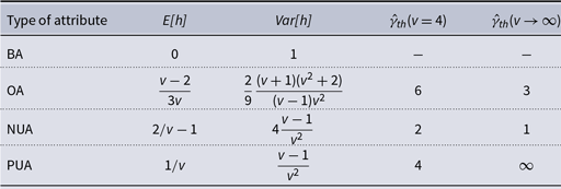
One can notice that the
 $\mathrm{E[}{h}\mathrm{]}$
equations for NUA and OA are the same as for BA when
$\mathrm{E[}{h}\mathrm{]}$
equations for NUA and OA are the same as for BA when
 $ v =$
2. The threshold
$ v =$
2. The threshold
 $\hat{\gamma }_{th}$
for BA is only defined for
$\hat{\gamma }_{th}$
for BA is only defined for
 $v=2$
and then it reaches
$v=2$
and then it reaches
 $\infty$
.
$\infty$
.
From the table, we can see that the number of categories
 $ v$
affects the expected value and the variance of similarity and weights. For
$ v$
affects the expected value and the variance of similarity and weights. For
 $ v \rightarrow \infty$
we derived the following dependencies:
$ v \rightarrow \infty$
we derived the following dependencies:
-
OA becomes a continuous attribute
$ \mathrm{E[}{h}\mathrm{]} = 1/3$
and
$ \mathrm{Var[}{h}\mathrm{]} = 2/9$
. Thus, an increase in
$ v$
leads to an increase in expected value and a decrease in variance, so fewer positive edges are destabilized, which leads to the decrease of local polarization. -
for NUA:
$ \mathrm{E[}{h}\mathrm{]} = -$
1 and
$ \mathrm{Var[}{h}\mathrm{]} =$
0. Any
$ \gamma \gt 1$
causes destabilization. The system reaches the state of hell. -
for PUA:
$ \mathrm{E[}{h}\mathrm{]} =$
0 and
$ \mathrm{Var[}{h}\mathrm{]} =$
0. Similarly as BA with large number of attributes
$G$
, the attribute layer has no influence on the relation layer. Destabilization never happens.


5.3 Impact of various types of attributes on destabilization and preventing
Figure 3 shows the effect of the number of attributes
 $G$
of different types on reduction of existing polarization (A) or preventing polarization (B) for different strengths of the attributes (
$G$
of different types on reduction of existing polarization (A) or preventing polarization (B) for different strengths of the attributes (
 $\gamma$
) in the case of complete graph structures. As predicted for scenario A, for too weak coupling strength
$\gamma$
) in the case of complete graph structures. As predicted for scenario A, for too weak coupling strength
 $ \gamma \lt 1$
, no system is destabilized. The local polarization
$ \gamma \lt 1$
, no system is destabilized. The local polarization
 $ P_{LP}$
is not equal to 1 because, in random balanced systems that contain only balanced triads, that is with 0 or 2 negative links, some of the former triads are present. The destabilization does not occur for BA at
$ P_{LP}$
is not equal to 1 because, in random balanced systems that contain only balanced triads, that is with 0 or 2 negative links, some of the former triads are present. The destabilization does not occur for BA at
 $ G =$
1 regardless of the value of
$ G =$
1 regardless of the value of
 $ \gamma$
(see the insets of Figure 3) because the attribute layer is also a balanced system in such a situation: with the appropriate coupling strength, the relation layer will change its initial balanced state to another balanced (probably polarized) state. In other cases above
$ \gamma$
(see the insets of Figure 3) because the attribute layer is also a balanced system in such a situation: with the appropriate coupling strength, the relation layer will change its initial balanced state to another balanced (probably polarized) state. In other cases above
 $ \gamma \gt$
1, as predicted, some systems are destabilized. In the case of BAs the destabilization becomes possible because the attribute layer contains both balanced and unbalanced triads when
$ \gamma \gt$
1, as predicted, some systems are destabilized. In the case of BAs the destabilization becomes possible because the attribute layer contains both balanced and unbalanced triads when
 $G\gt 1$
.
$G\gt 1$
.
Destabilizing the system with NUA is related to reaching the state of hell. This is evidenced by the high
 $P_{LP}$
(i.e., high densities of triangles with 2 or 3 negative links; see also Figure 2 in SM). The increase in local polarization for NUA is caused by the negative expected value of attribute layer weights
$P_{LP}$
(i.e., high densities of triangles with 2 or 3 negative links; see also Figure 2 in SM). The increase in local polarization for NUA is caused by the negative expected value of attribute layer weights
 $ \mathrm{E[}{h}\mathrm{]} \lt 0$
, which leads to more frequent destabilization of positive links than negative links. For other attributes, looking at the polarization figures, you can see that for attributes with a positive expected value of
$ \mathrm{E[}{h}\mathrm{]} \lt 0$
, which leads to more frequent destabilization of positive links than negative links. For other attributes, looking at the polarization figures, you can see that for attributes with a positive expected value of
 $ \mathrm{E[}{h}\mathrm{]}\gt 0$
(i.e., OA and PUA), high
$ \mathrm{E[}{h}\mathrm{]}\gt 0$
(i.e., OA and PUA), high
 $ \gamma$
strengths effectively limit the polarization and lead to the paradise state. For BA and for the couplings lower than the threshold
$ \gamma$
strengths effectively limit the polarization and lead to the paradise state. For BA and for the couplings lower than the threshold
 $ \gamma \lt \hat{\gamma }_{th}$
for OA and PUA, the considered measures of polarization return to the baseline as the number of attributes increases. In such cases, the attributes are of less and less importance.
$ \gamma \lt \hat{\gamma }_{th}$
for OA and PUA, the considered measures of polarization return to the baseline as the number of attributes increases. In such cases, the attributes are of less and less importance.
Thus, the results confirm the existence of threshold values of strength as discussed in Section 5.2. For attributes with positive
 $\mathrm{E[}{h}\mathrm{]}$
, for
$\mathrm{E[}{h}\mathrm{]}$
, for
 $ \gamma \gt 1$
, as the number of attributes increases, first we observe the decrease of polarization, and then depending whether
$ \gamma \gt 1$
, as the number of attributes increases, first we observe the decrease of polarization, and then depending whether
 $ \gamma \lt \hat{\gamma }_{th}$
or
$ \gamma \lt \hat{\gamma }_{th}$
or
 $ \gamma \gt \hat{\gamma }_{th}$
, we either observe an increase and return to the baseline polarization, or a further decrease up to reaching a paradise state, respectively. For negative unordered attributes, we have
$ \gamma \gt \hat{\gamma }_{th}$
, we either observe an increase and return to the baseline polarization, or a further decrease up to reaching a paradise state, respectively. For negative unordered attributes, we have
 $\mathrm{E[}{h}\mathrm{]}\lt 0$
, therefore we observe a symmetric, but opposite behavior (i.e., more attributes make the state more polarized, exceeding
$\mathrm{E[}{h}\mathrm{]}\lt 0$
, therefore we observe a symmetric, but opposite behavior (i.e., more attributes make the state more polarized, exceeding
 $\hat{\gamma }_{th}$
results eventually in reaching the state of hell, etc.). A small number of binary attributes slightly lowers polarization; however, as
$\hat{\gamma }_{th}$
results eventually in reaching the state of hell, etc.). A small number of binary attributes slightly lowers polarization; however, as
 $\mathrm{E[}{h}\mathrm{]}=0$
, a further increase of
$\mathrm{E[}{h}\mathrm{]}=0$
, a further increase of
 $ G$
makes the attributes matter less and less, which stops efficient destabilization or prevention.
$ G$
makes the attributes matter less and less, which stops efficient destabilization or prevention.
Looking at Scenario B in Figure 3, we see that attributes have a bigger impact on preventing than on destabilizing the polarized state. This is mostly due to (which applies broadly to all Figures 3–5) an increased basin of attraction for unpolarized states given random initial conditions (i.e., when initial conditions are random, the network is less likely to fall into a polarized state, especially as number of nodes increases). For the prevention problem, the baseline level of
 $P_{LP}$
that is reached for larger
$P_{LP}$
that is reached for larger
 $G$
depends on the attribute type’s expected value
$G$
depends on the attribute type’s expected value
 $\mathrm{E[}{h}\mathrm{]}$
. For binary attributes (
$\mathrm{E[}{h}\mathrm{]}$
. For binary attributes (
 $\mathrm{E[}{h}\mathrm{]}=0$
) there is no visible difference between scenarios. Positive or negative
$\mathrm{E[}{h}\mathrm{]}=0$
) there is no visible difference between scenarios. Positive or negative
 $\mathrm{E[}{h}\mathrm{]}$
make the system less or more polarized, respectively. Smaller couplings
$\mathrm{E[}{h}\mathrm{]}$
make the system less or more polarized, respectively. Smaller couplings
 $\gamma$
, as compared to destabilization scenario, are sufficient to bring the systems to paradise or hell states. Assuming
$\gamma$
, as compared to destabilization scenario, are sufficient to bring the systems to paradise or hell states. Assuming
 $\mathrm{E[}{h}\mathrm{]}\gt 0$
, there is no negative effect of increasing the number of attributes for any value of coupling, as we do not observe the threshold
$\mathrm{E[}{h}\mathrm{]}\gt 0$
, there is no negative effect of increasing the number of attributes for any value of coupling, as we do not observe the threshold
 $\hat{\gamma }_{th}$
. Thus, in such a case having more attributes ensures smaller polarization.
$\hat{\gamma }_{th}$
. Thus, in such a case having more attributes ensures smaller polarization.
Differences between the effect of attributes for the two scenarios are also marked in Figure 4, where the entire range of attribute layer strength (
 $\gamma$
) is compared. Selecting
$\gamma$
) is compared. Selecting
 $\gamma \lt 1$
is not enough to destabilize a polarized state, but may sufficiently prevent polarization from occurring. With high coupling values, the attribute impact is the same. The destabilization or prevention of a polarized system occurs most effectively (in order according to the lowest required strength) for CA, PUA, OA, and BA. NUA can reduce the global polarization (see Figure 4 in SM), but it always leads to an increase of local polarization within the system.
$\gamma \lt 1$
is not enough to destabilize a polarized state, but may sufficiently prevent polarization from occurring. With high coupling values, the attribute impact is the same. The destabilization or prevention of a polarized system occurs most effectively (in order according to the lowest required strength) for CA, PUA, OA, and BA. NUA can reduce the global polarization (see Figure 4 in SM), but it always leads to an increase of local polarization within the system.

Figure 4. Preventing (B) from forming as compared to destabilizing (A) polarized states requires smaller strength. The panels show the local polarization measure
 $ P_{LP}$
as a function of attribute layer strength
$ P_{LP}$
as a function of attribute layer strength
 $\gamma$
for
$\gamma$
for
 $ N =$
9 and
$ N =$
9 and
 $ G =$
5, for different types of attributes, for complete graph networks.
$ G =$
5, for different types of attributes, for complete graph networks.
Figure 5 shows that the local polarization decreases with growing system size
 $N$
. The curves on the BA charts (i.e., OA for
$N$
. The curves on the BA charts (i.e., OA for
 $ v =$
2), OA for
$ v =$
2), OA for
 $ v =$
4 and CA (i.e., OA for
$ v =$
4 and CA (i.e., OA for
 $ v =$
1000) change monotonically with the increasing number of categories. The larger
$ v =$
1000) change monotonically with the increasing number of categories. The larger
 $ v$
, the smaller the polarization of the system (see also Figure 3 in SM). This observation goes along with the conclusions from Table 2, because with increasing expected value
$ v$
, the smaller the polarization of the system (see also Figure 3 in SM). This observation goes along with the conclusions from Table 2, because with increasing expected value
 $\mathrm{E[}{h}\mathrm{]}$
, decreasing polarization becomes easier. For PUA (and partially CA) and high coupling strengths, the lack of polarization is tantamount to the system reaching paradise. It is surprising that having an intermediate coupling strength slightly exceeding 1 (e.g.,
$\mathrm{E[}{h}\mathrm{]}$
, decreasing polarization becomes easier. For PUA (and partially CA) and high coupling strengths, the lack of polarization is tantamount to the system reaching paradise. It is surprising that having an intermediate coupling strength slightly exceeding 1 (e.g.,
 $\gamma =1.5$
), unordered attributes are worse at destabilization of the polarized state. This is not true for scenario B. For the intermediate threshold, all the attributes reduce global polarization (see Figure 5 in SM), but the consequence of NUA is an increase in local polarization.
$\gamma =1.5$
), unordered attributes are worse at destabilization of the polarized state. This is not true for scenario B. For the intermediate threshold, all the attributes reduce global polarization (see Figure 5 in SM), but the consequence of NUA is an increase in local polarization.
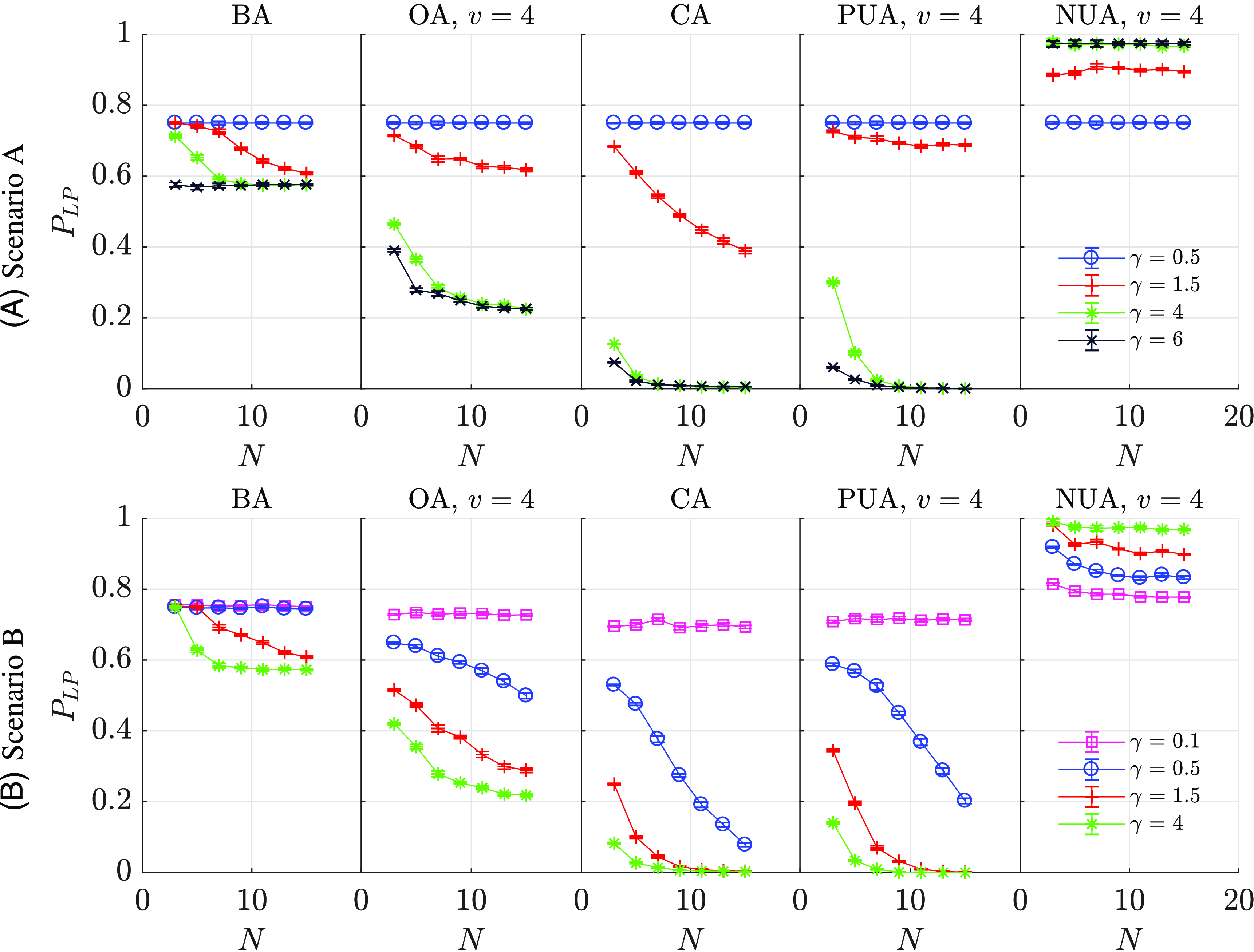
Figure 5. Same conditions of attributes for growing systems of size
 $N$
lead to approximately lower local polarization
$N$
lead to approximately lower local polarization
 $P_{LP}$
. Panels show scenarios of (A) destabilization and (B) preventing, respectively, for
$P_{LP}$
. Panels show scenarios of (A) destabilization and (B) preventing, respectively, for
 $G=5$
of different types of attributes and different strengths.
$G=5$
of different types of attributes and different strengths.
Having a certain number of attributes of a given type, it is not always possible to eliminate polarization completely (i.e., achieve paradise) by simply increasing the attribute layer influence
 $\gamma$
. For extremely large couplings there is a limit, that is, an average polarization level one achieves having a certain type and number of attributes. This limit can be larger than 0. For instance, as shown in Figure 3, with BAs one cannot decrease the polarization on average below
$\gamma$
. For extremely large couplings there is a limit, that is, an average polarization level one achieves having a certain type and number of attributes. This limit can be larger than 0. For instance, as shown in Figure 3, with BAs one cannot decrease the polarization on average below
 $P_{LP}=0.5$
no matter other parameters. For OAs (
$P_{LP}=0.5$
no matter other parameters. For OAs (
 $v=4$
,
$v=4$
,
 $G=5$
) with high coupling paradise is not reached but
$G=5$
) with high coupling paradise is not reached but
 $P_{LP} \approx 0.23$
. Similar levels that agree with these analytic curves are also visible in Figures 4 and 5.
$P_{LP} \approx 0.23$
. Similar levels that agree with these analytic curves are also visible in Figures 4 and 5.
5.4 Destabilization and prevention of polarization in real-world network structures
The impact of attributes on scenarios A and B in the case of increasing
 $\gamma$
strength does not depend on the network topology as the obtained results for the complete graph (Figure 4) and the high school network structure (Figure 6) are almost the same. One can only notice that for the high school topology, probably due to the larger system size, smaller strength is required to reach the plateau level of
$\gamma$
strength does not depend on the network topology as the obtained results for the complete graph (Figure 4) and the high school network structure (Figure 6) are almost the same. One can only notice that for the high school topology, probably due to the larger system size, smaller strength is required to reach the plateau level of
 $P_{LP}$
. The same observation is made when comparing other analyzed characteristics (Figure 3 and SM, Figure 7). Thus, we confirm that a complete graph is a good approximation of a small community network in this model. The previously obtained conclusions are valid also for other networks that do not display community structure.
$P_{LP}$
. The same observation is made when comparing other analyzed characteristics (Figure 3 and SM, Figure 7). Thus, we confirm that a complete graph is a good approximation of a small community network in this model. The previously obtained conclusions are valid also for other networks that do not display community structure.
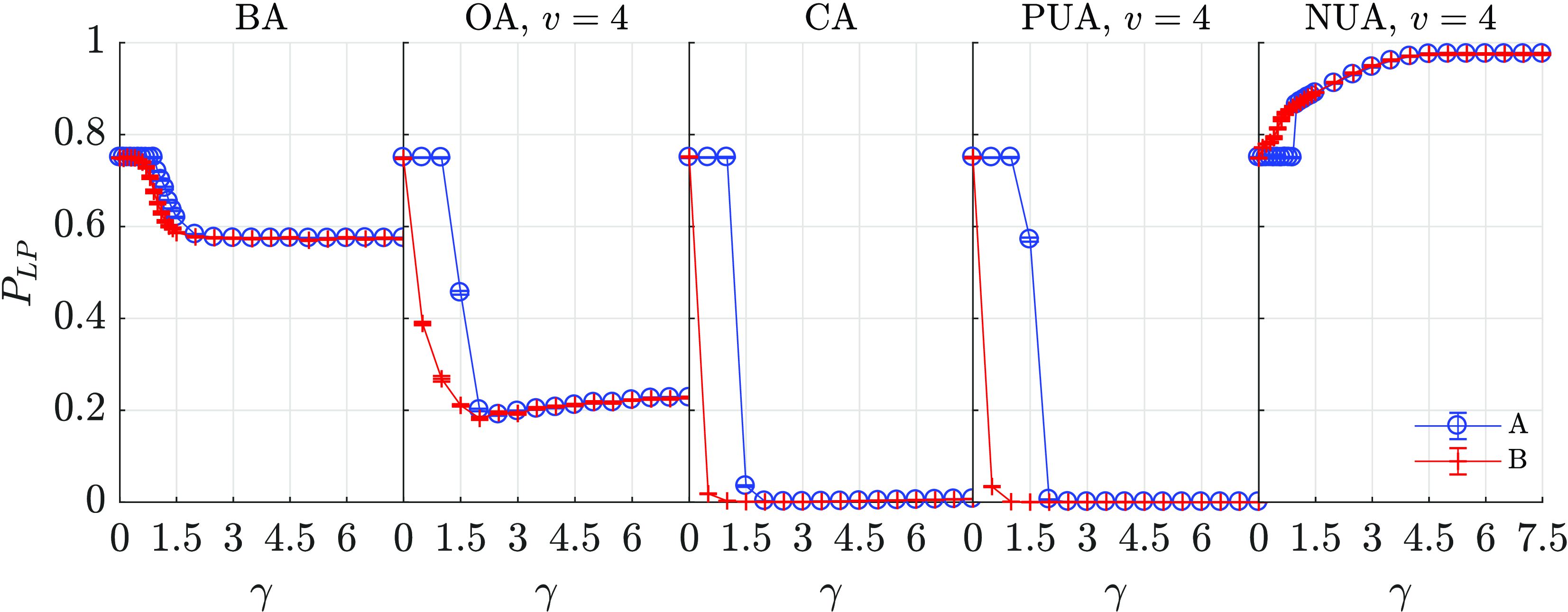
Figure 6. No significant changes in the results for a real-world network structure as compared to a complete graph topology. Similarly to Figure 4, the plots show local polarization measure
 $P_{LP}$
as a function of the strength
$P_{LP}$
as a function of the strength
 $\gamma$
for the scenarios of (A) destabilization and (B) preventing from forming a polarized state. The underlying network is a structure of face-to-face contacts between high school classmates.
$\gamma$
for the scenarios of (A) destabilization and (B) preventing from forming a polarized state. The underlying network is a structure of face-to-face contacts between high school classmates.
However, an unexpected result is obtained when the underlying topology contains a community structure. Figure 7a shows the change of local polarization when more and more attributes are considered to influence the relation layer in the case of ZKC network topology. The obtained level of polarization in the system without the attributes (i.e., when
 $\gamma \lt 1$
) is surprisingly low. The reason for that is the low number of edges between the two groups (see ZKC network graph in SM, Figure 3b) and, as a consequence, the initially low number of polarized triads. When comparing this plot to Figure 3a, it may seem that not only do negative unordered attributes increase polarization, but also that using binary attributes or small numbers of ordered and continuous attributed has a detrimental effect on the destabilization of polarization. However, the opposite conclusion comes from Figure 7b, where for the same network the probability
$\gamma \lt 1$
) is surprisingly low. The reason for that is the low number of edges between the two groups (see ZKC network graph in SM, Figure 3b) and, as a consequence, the initially low number of polarized triads. When comparing this plot to Figure 3a, it may seem that not only do negative unordered attributes increase polarization, but also that using binary attributes or small numbers of ordered and continuous attributed has a detrimental effect on the destabilization of polarization. However, the opposite conclusion comes from Figure 7b, where for the same network the probability
 $P_{GP}$
of reaching global polarization is shown. Having a weak influence of attributes
$P_{GP}$
of reaching global polarization is shown. Having a weak influence of attributes
 $\gamma \lt 1$
, the system always stays globally polarized. All kinds of attributes are able to destabilize the system. Looking at different numbers
$\gamma \lt 1$
, the system always stays globally polarized. All kinds of attributes are able to destabilize the system. Looking at different numbers
 $G$
and strengths
$G$
and strengths
 $\gamma$
, the most beneficial are CAs, followed by PUAs, BAs and OAs (both giving similar effect), and NUAs as the least effective. Actually, the impacts of attributes on global polarization probability in the cases of ZKC and complete graph topologies are very similar (see SM, Figure 2c for comparison).
$\gamma$
, the most beneficial are CAs, followed by PUAs, BAs and OAs (both giving similar effect), and NUAs as the least effective. Actually, the impacts of attributes on global polarization probability in the cases of ZKC and complete graph topologies are very similar (see SM, Figure 2c for comparison).

Figure 7. In networks with distinct communities, destabilization of a polarized state is still possible, but sometimes at the cost of increasing local tensions. Panels (a) and (c) show the local polarization metric
 $P_{LP}$
as a function of number of attributes
$P_{LP}$
as a function of number of attributes
 $G$
for Zachary karate club and Windsurfers networks, respectively. Panel (b) displays the probability
$G$
for Zachary karate club and Windsurfers networks, respectively. Panel (b) displays the probability
 $P_{GP}$
of obtaining global polarization for Zachary karate club network. Although local tensions increased (panel a), a globally polarized state is less frequently achievable (panel b).
$P_{GP}$
of obtaining global polarization for Zachary karate club network. Although local tensions increased (panel a), a globally polarized state is less frequently achievable (panel b).
From this, we see a connection between an increase in local polarization and a decrease in global polarization. The measure
 $P_{LP}$
takes only into account separate triadic motifs whereas the probability
$P_{LP}$
takes only into account separate triadic motifs whereas the probability
 $P_{GP}$
treats the structure of the whole network as one consistent object. Therefore, in the case of systems consisting of distinct communities, both measures of polarization should be included in the analysis. For NUAs, either the system usually reaches a globally polarized state (
$P_{GP}$
treats the structure of the whole network as one consistent object. Therefore, in the case of systems consisting of distinct communities, both measures of polarization should be included in the analysis. For NUAs, either the system usually reaches a globally polarized state (
 $P_{GP}$
close to 1) or most of the links are negative. For binary attributes or small numbers of ordered or continuous attributes one cannot destroy the globally polarized state without introducing some tensions (i.e., polarized triads) inside the initially divided communities. On the other hand, even a small number of positive unordered attributes reduces both polarization metrics.
$P_{GP}$
close to 1) or most of the links are negative. For binary attributes or small numbers of ordered or continuous attributes one cannot destroy the globally polarized state without introducing some tensions (i.e., polarized triads) inside the initially divided communities. On the other hand, even a small number of positive unordered attributes reduces both polarization metrics.
Similar results are also obtained for the Windsurfers network (Figure 7c). The initial level of local polarization is larger, which shows that the connections between the two communities are more frequent. Again, BAs or small number of OAs are enough to completely eradicate the globally polarized state (see SM, Figure 9 for
 $P_{GP}$
relation) but at the same time, the increase of local polarization is observed. This time CAs and PUAs can be used to decrease both the local and global polarization.
$P_{GP}$
relation) but at the same time, the increase of local polarization is observed. This time CAs and PUAs can be used to decrease both the local and global polarization.
Above we described the influence of attributes related to scenario A. The results related to scenario B in the networks with communities are shown only in SM, Figure 8. We do not observe any significant differences as compared to Figure 3b. Communities do not influence the rise of polarization shortly after networks are formed.
6. Discussion and conclusions
The general model and simulation framework that we presented is sufficient to allow us to draw conclusions about how different types of attributes may impact polarization in a network. From this, we are able to characterize the types of changes likely to occur in the network as well as the strength of emphasis needed on the attributes to create substantial change in the relationships. This model is consistent with both structural balance and homophily theories. The model allows us to learn about traits in general, traits relative to each other, and about particular traits as well. One of the advances of this modeling framework is that we connect the ideas of structural balance and polarization, which requires redefining some aspects of each, allowing us to use models of structural balance to study polarization.
We can learn about the general effect of attributes on relationships through both analytical reasoning and statistical analysis. If the strength of the distance function between attributes is not big enough (i.e.,
 $|g_{ij}| \lt 1$
), then a lot of emphasis will need to be placed on the attributes to destabilize the relationship layer (i.e.,
$|g_{ij}| \lt 1$
), then a lot of emphasis will need to be placed on the attributes to destabilize the relationship layer (i.e.,
 $\gamma \gt 1$
). Furthermore, if we want to destabilize a particular link in a network, we will be able to do so if the signs of weights in the relation and attribute layers are not the same and there is a strong enough emphasis placed on the attribute layer—that is, Equation (9). Since that will not ensure a permanently destabilized network, we can do so by ensuring that at least one triad is unpolarized, which can be achieved when [see Equation (10)] the emphasis placed on the attributes is sufficient (i.e.,
$\gamma \gt 1$
). Furthermore, if we want to destabilize a particular link in a network, we will be able to do so if the signs of weights in the relation and attribute layers are not the same and there is a strong enough emphasis placed on the attribute layer—that is, Equation (9). Since that will not ensure a permanently destabilized network, we can do so by ensuring that at least one triad is unpolarized, which can be achieved when [see Equation (10)] the emphasis placed on the attributes is sufficient (i.e.,
 $|\gamma g_{ij} | \gt 1$
), and either there is at least some social tension in the triad (i.e., the triad is unbalanced with one negative link) or there are only positive links connecting the triad’s agents.
$|\gamma g_{ij} | \gt 1$
), and either there is at least some social tension in the triad (i.e., the triad is unbalanced with one negative link) or there are only positive links connecting the triad’s agents.
This framework also allows us to make claims about the effect of attributes relative to one another (remembering, of course, that we have not exhaustively defined all attributes). In order to destabilize or prevent polarization, attributes are most effective in descending order (assuming four categories where applicable): continuous attributes, positive unordered attributes, ordered attributes, binary attributes (with an important caveat discussed below), and negative unordered attributes. One important way of restating the above is that for a given collection of attributes (e.g., number of attributes and categories), the emphasis on the attribute layer needed to destabilize the polarization decreases according to the list. This means that if placing emphasis on the attribute layer is costly (e.g., a business seeks to disrupt polarization in a work group), then costs will be lower by focusing on traits in the order presented above. One interesting difference between the types of traits is that positive unordered traits are more likely to lead to paradise than ordered traits while ordered traits are more likely to have diverse triads.
In general, for attributes for which a probability density function and a mean can be found, we obtained some expectations for how they will impact polarization. These expectations were met for the specific types of attributes tested using our framework. If the mean is less than 0 (e.g., for negative unordered attributes), attributes may destabilize global polarization but, at the same time, they increase local polarization, eventually, with sufficient emphasis, leading to a state of hell (all links negative). That is the reason why we have not considered negative unordered attributes as contributing much to decreases in polarization, because we understand polarization so as the state with many negative links to be a social state that makes coordination between people more difficult. If the mean is 0, attributes may lower polarization to some small extent, though it may not be enough to destabilize a polarized system. An example is binary attributes. A small number of them decreases polarization, but a large number has no effect. A similar effect was observed in (Pham et al., Reference Pham, Korbel, Hanel and Thurner2022), where balanced states are more difficult to achieve when having more binary attributes. For a special case of one binary attribute, the polarization also is not lowered, because the network may change one polarized state into another one (Altafini, Reference Altafini2012). If the mean is positive, then attributes have the potential to destabilize and prevent polarization as long as the emphasis on them is strong enough. This is the case for positive unordered, ordered and continuous attributes types. This finding is also in agreement with the results obtained in Schweighofer et al. (Reference Schweighofer, Schweitzer and Garcia2020b), where in a different model unpolarized states are more probable when there are more continuous attributes. While many systems with positive mean approach paradise with a high enough
 $\gamma$
, they all need an emphasis greater than the theoretical minimum to destabilize polarization (i.e.,
$\gamma$
, they all need an emphasis greater than the theoretical minimum to destabilize polarization (i.e.,
 $\gamma \ge 1$
). Intriguingly, this suggests there may exist an attribute type that is more effective at depolarizing a network (i.e.,
$\gamma \ge 1$
). Intriguingly, this suggests there may exist an attribute type that is more effective at depolarizing a network (i.e.,
 $\gamma$
approaching 1 from the right would be sufficient enough to see substantial polarization drop). The effect of the number of categories goes in opposite directions for unordered and ordered attributes. As the number of categories in an unordered attribute increases, the less likely it is to destabilize polarization – in the extreme example, every person is completely unique. For ordered attributes, however, increasing the number of categories increases how effective the attribute is at destabilizing polarization until, at the extreme end, it is a continuous attribute.
$\gamma$
approaching 1 from the right would be sufficient enough to see substantial polarization drop). The effect of the number of categories goes in opposite directions for unordered and ordered attributes. As the number of categories in an unordered attribute increases, the less likely it is to destabilize polarization – in the extreme example, every person is completely unique. For ordered attributes, however, increasing the number of categories increases how effective the attribute is at destabilizing polarization until, at the extreme end, it is a continuous attribute.
Our results fit into previous research on the topic where it was shown that binary attributes were the most effective in limiting structural balance (Du et al., Reference Du, He and Feldman2016) while continuous attributes led to an increased abundance of structural balance (Gao and Wang, Reference Gao and Wang2018). In our model, we have obtained complementary results (see section 4.3 in SM) for binary and continuous attributes and also explored other attribute types. The difference between these previous findings and our main finding that continuous attributes effectively destabilize and prevent polarization shows that most of the impact of continuous attributes on increasing structural balance comes from such attributes leading to a state of paradise.
Our study shows that preventing polarization from forming is easier than destabilizing a balanced (usually polarized) state. Even a small strength of the attribute layer may be sufficient to prevent polarization. Moreover, in such a case increasing the number of attributes does not worsen the attribute effect. The above observations are not true when the goal is to destabilize the initial system. First, as already mentioned a necessary condition for the destabilization is facilitating the attribute layer to be more influential than the relation layer. Second, even if above condition is fulfilled but the attribute layer coupling strength does not exceed the analytically calculated threshold level
 $\hat{\gamma }_{th}$
, then too many attributes make the destabilization less effective. Apart from that, for both considered scenarios, it was observed that the larger the number of nodes in the network, the easier the tasks of prevention and destabilization are.
$\hat{\gamma }_{th}$
, then too many attributes make the destabilization less effective. Apart from that, for both considered scenarios, it was observed that the larger the number of nodes in the network, the easier the tasks of prevention and destabilization are.
Preventing polarization does not depend on the underlying network structure. On the contrary, destabilization is affected when the initial polarization goes together with distinct communities in existing relations. In that case, attributes such as binary or ordered attributes may lead to opposite effects in terms of local and global polarization. Namely, in order to decrease global polarization in networks already divided into communities, it might be necessary to introduce some conflict into those communities. This corresponds to observations that diversity and community are usually negatively correlated (Neal and Neal, Reference Neal and Neal2014; Stivala et al., Reference Stivala, Robins, Kashima and Kirley2016). This could result in negative reactions to efforts to reduce polarization as they may increase local polarization.
The presented model and results were obtained by using a number of assumptions some of which were given in Sections 2.1 and 4.2. Those assumptions are necessary simplifications that allow us to draw conclusions from the model. Probably the most significant assumption is taking into account only the impact of the attribute layer on the relation layer. This is related to assuming that attributes change much slower than relations, as it is in the case of immutable attributes, like race, or in the case of attributes that change at a slow rate (e.g., place of living, religion, wealth). Due to this assumption, the attribute layer is static and acts as a controller for the subordinate relation layer. In a more complex model, a bilateral coupling would have to be considered, as in the model in (Górski et al., Reference Górski, Kułakowski, Gawroński and Hołyst2017). This would be a natural extension of this research. For the presented model, however, we can consider any attribute of an individual as long as it changes much slower than relationships. This will include some traditionally considered opinions (e.g., political preference) but may not include other opinions (e.g., best mid-tier restaurant in the city). Importantly, this makes whether or not something can be considered an attribute an empirical question: does that aspect of individuals change much more slowly than relationships between individuals?
The limitation of our model is that relations either exist or do not; new relations are not created during the simulation. Only the initially existing ones evolve. Moreover, these relations tend to become either positive or negative. They cannot become neutral. One way to overcome this is introducing rates of link creation and disappearance that could depend on agents’ common neighbors or the current value of the relation. Neutral links would also become possible if the model evolution became dependent on noise (Malarz and Hołyst, Reference Malarz and Hołyst2022), which would require changing the structural balance term of Equation (1). We also assume the indirect relations between agents. Agents both like or dislike each other the same way and the influence of similarity is indirect (
 $g_{ij}=g_{ji}$
). However, the model of relation evolution could easily be extended to directed networks (Krawczyk et al., Reference Krawczyk, del Castillo-Mussot, Hernández-Ramírez, Naumis and Kułakowski2015). Nonreciprocal similarities require either nonhomogeneous agents for whom different attributes would be of different importance or attributes with a nonsymmetrical similarity function. An example is an attribute related to status theory (Leskovec et al., Reference Leskovec, Huttenlocher and Kleinberg2010a). People would tend to have positive relations with those of higher status and negative ones with those of lower status.
$g_{ij}=g_{ji}$
). However, the model of relation evolution could easily be extended to directed networks (Krawczyk et al., Reference Krawczyk, del Castillo-Mussot, Hernández-Ramírez, Naumis and Kułakowski2015). Nonreciprocal similarities require either nonhomogeneous agents for whom different attributes would be of different importance or attributes with a nonsymmetrical similarity function. An example is an attribute related to status theory (Leskovec et al., Reference Leskovec, Huttenlocher and Kleinberg2010a). People would tend to have positive relations with those of higher status and negative ones with those of lower status.
One of the ways that we can extend this model is to relax assumptions about the attributes. If we were to relax the assumption that the similarity measure is maximized when the individuals share a value of an attribute, this would allow for attributes where people are drawn to those who are different than themselves. This might arise, for example, in a case of social niche specialization (Bergmüller and Taborsky, Reference Bergmüller and Taborsky2010) where people are trying to create a group that allows each person to have a unique social role, thereby minimizing conflict. Relaxing other assumptions may allow us to analyze additional types of relationships and attributes.
Here, we studied the impact of attributes of only one kind in a model. It would be interesting to evaluate the inter-relations between different types of attributes. A combination of a negative ordered (or binary) attribute and a continuous attribute (proximity between places of living) were considered by Neal and Neal (Reference Neal and Neal2014) and Stivala et al. (Reference Stivala, Robins, Kashima and Kirley2016). A single unordered attribute lead to polarization defined as highly clustered and internally dense communities. On the other hand, a single continuous attribute facilitated community interlinks and, therefore, decreased polarization. We also assumed that attributes are not correlated, have the same importance, and all possible categories are drawn from a uniform distribution. However, our conclusions can be extrapolated to cases not covered by those assumptions. In reality, the attributes are usually correlated. Having correlated attributes in our model would decrease the effective number of attributes. Thus, following Figure 3 which shows nonmonotonic changes, the consequence of correlated attributes will depend on the parameters. For example, if all the binary attributes are perfectly correlated (i.e., there is one effective attribute), then they do not decrease the polarization but lead to a different polarized state. But if there are more effective binary attributes, we will obtain a less polarized state as compared to the system with uncorrelated attributes. If attribute categories are drawn from a different distribution, for example from a normal distribution, it also does not change the obtained conclusions. For such attributes, we can still calculate (either analytically or numerically) the expected value of the similarity and use the previously mentioned conclusions related to the sign of the expected value.
Groups that we considered in this paper are networks of people and we analyzed polarization among humans. However, it is also possible to extend this model to the case of networks of countries (Antal et al., Reference Antal, Krapivsky and Redner2005; Doreian and Mrvar, Reference Doreian and Mrvar2015). In such a case, the attributes could be, for example, popular sports, main industries, religion. Our framework could be used to predict the changes of relations, although it is unclear whether reducing polarization at this level is attainable.
6.1 Practical implications
These results have immediately useful application to problems of interest to institutions and social groups. From a practical point of view, if we want to reduce tensions in a conflicted community, we should highlight attributes that have shared values in conflicted groups, which would allow the creation of many positive mediating links between groups (Du et al., Reference Du, He, Wang and Feldman2018; Rawlings, Reference Rawlings2022). Businesses can use these results to improve cohesion in their working groups. Most business teams are small enough (7–9 people) that everyone knows each other and has relationships. Consequently, this can lead to the formation of polarized groups with negative consequences for the entire team. Suppose the company is able to identify attributes that have on average a positive impact on the relation layer (e.g., continuous attributes) and appear fairly evenly in both groups. In that case, it will be possible to dedicate relatively fewer resources to emphasize these attributes than if, for example, a binary attribute was selected. The company can do even better by emphasizing more of these attributes, requiring a lower investment.
Another example would be the question of reducing the polarization present in society. We can envision an advertisement campaign in the United States that is something like, “Democrats get lung cancer just like Republicans.” Or one in Britain that is something like, “Remainers play football too.” Emphasizing positive unordered attributes (e.g., hobbies, diseases) highlights similarities across polarized groups, hopefully decreasing polarization. The proposed model shows that the more people see themselves through attributes of this type, the more they will create a less polarized community. This is in agreement with the results from recent papers of Levendusky (Reference Levendusky2018) and Rawlings (Reference Rawlings2022) where it was noticed that perceiving others through a common shared attribute or having more crosscutting ties facilitates reduction of polarization that arose from division of the society into two partisan camps.
Finally, the result of this work may also show the mechanism of increasing polarization in society due to the rise of the Internet. It is not simply that you can find more people who think similarly to you, therefore creating echo chambers. Rather, the impact of many attributes that previously cut across political affiliation (such as income, race, hobbies) has decreased because people who only know each other through the internet tend to know little about their partners. We can describe this phenomenon using our model. Such attributes would not be present, or their significance would be lowered by decreasing the
 $ C_g$
variable, only for these features. When the only significant attributes left are those related to politics, only these attributes determine the signs of connections between the members of a given group. Needless to say, these attributes most closely resemble the negative unordered attributes (Huber and Malhotra, Reference Huber and Malhotra2017). In effect, this leads to system polarization. On the other hand, enabling people to learn attributes of others, if they share attributes, instantly creates positive connections that reduce polarization even during considerations of a partisan topic (Balietti et al., Reference Balietti, Getoor, Goldstein and Watts2021).
$ C_g$
variable, only for these features. When the only significant attributes left are those related to politics, only these attributes determine the signs of connections between the members of a given group. Needless to say, these attributes most closely resemble the negative unordered attributes (Huber and Malhotra, Reference Huber and Malhotra2017). In effect, this leads to system polarization. On the other hand, enabling people to learn attributes of others, if they share attributes, instantly creates positive connections that reduce polarization even during considerations of a partisan topic (Balietti et al., Reference Balietti, Getoor, Goldstein and Watts2021).
The results presented here could immediately be applied at relevant levels to decrease polarization. This general framework could be extended by including additional attribute types, allowing us to better decrease polarization. The model could also be extended to allow feedback between relationships and attributes. The flexibility and versatility of this framework can make it useful to both researchers and policymakers.
Competing interests
None.
Funding statement
This work was supported by Polish National Science Center, grant Alphorn no. 2019/01/Y/ST2/00058. J.A.H. was partially supported by OMINO Project from the European Union’s Horizon 2021 research and innovation program under the Marie Skłodowska-Curie Grant Agreement No. 101086321.
Data availability statement
Simulation framework code was made open source. It allows anybody to use our framework and to test other attributes and/or different scenarios. The code is available in https://github.com/pjgorski/PolarizationFramework.
Supplementary material
The supplementary material for this article can be found at https://doi.org/10.1017/nws.2023.13.


 Open access