


1. Introduction
Most of the observed ice-mass loss in Antarctica over the last decades has been attributed to increased heat transport from the ocean resulting in ice-shelf thinning and ice-stream acceleration (Schmidtko and others, Reference Schmidtko, Heywood, Thompson and Aoki2014; Paolo and others, Reference Paolo, Fricker and Padman2015; Rignot and others, Reference Rignot2019). Ice shelves surround ~70% of the Antarctic continent (Bindschadler and others, Reference Bindschadler2011) and buttress ice transport from the interior towards the ocean (Dupont and Alley, Reference Dupont and Alley2005; Gudmundsson, Reference Gudmundsson2013; Fürst and others, Reference Fürst2016). Further corroborating the buffering effect of ice shelves are areas where ice shelves are grounded, i.e. at ice rises and ice rumples (Matsuoka and others, Reference Matsuoka2015; Berger and others, Reference Berger, Favier, Drews, Derwael and Pattyn2016; Goel and others, Reference Goel2020). It has been shown that these pinning points can delay grounding-line retreat of the Antarctic marine ice sheets (Favier and others, Reference Favier, Pattyn, Berger and Drews2016). In order to improve current assessments and predictions of Antarctica's ice mass loss, not only the presence but also the internal structure of ice marginal features needs to be known. Hereby the internal stratigraphy of ice shelves provides an integrated memory of the atmospheric-, oceanographic- and ice dynamic history (Das and others, Reference Das2020; Drews and others, Reference Drews2020). For ice rises, prior information about areas where the stratigraphy is flat and continuous would allow for the identification of suitable ice core-drilling locations (Steig and others, Reference Steig2006).
The internal ice stratigraphy can be obtained by mapping internal reflection horizons (IRHs). IRHs represent interfaces of dielectric contrasts originating from impurities on former snow surfaces that were buried and subsequently deformed by ice flow (Eisen and others, Reference Eisen, Nixdorf, Wilhelms and Miller2004). Antarctica's ice-sheet stratigraphy has been extensively mapped by airborne radars over the grounded ice-sheet interior (e.g. Karlsson and others, Reference Karlsson, Rippin, Vaughan and Corr2009; Winter and others, Reference Winter, Steinhage, Creyts, Kleiner and Eisen2019; Ashmore and others, Reference Ashmore2020; Schroeder and others, Reference Schroeder2020; Cavitte and others, Reference Cavitte2021). IRH data are increasingly becoming publicly available (Winter and others, Reference Winter, Steinhage, Creyts, Kleiner and Eisen2019; Ashmore and others, Reference Ashmore2020; Bodart and others, Reference Bodart2021; Cavitte and others, Reference Cavitte2021), and cross-system calibrations indicate that some IRHs appear similar in different radar systems (Winter and others, Reference Winter2017; Cavitte and others, Reference Cavitte2021). More recent studies have also focused on Antarctica's ice marginal areas (e.g. Das and others, Reference Das2020; Bodart and others, Reference Bodart2021) and current scientific community efforts are planning to further expand these datasets, e.g. the SCAR Scientific Research Program INStabilities & Thresholds in ANTarctica (INSTANT) or SCAR Action Groups, such as AntArchitecture (Bingham and others, Reference Bingham2020) and RINGS (Matsuoka and others, Reference Matsuoka, Forsberg, Ferraccioli, Moholdt and Morlighem2022).
In Antarctica, most mapping of IRHs is focused on Antarctica's interior, particularly near the deep ice core-drilling sites where the stratigraphy is well preserved (e.g. Ashmore and others, Reference Ashmore2020; Cavitte and others, Reference Cavitte2021; Van Liefferinge and others, Reference Van Liefferinge2021). However, in coastal areas the ice stratigraphy generally has more variable patterns. Here, IRH geometries are shaped by processes operating on small spatial scales, e.g. across the grounding line where ice dynamics, surface accumulation (Lenaerts and others, Reference Lenaerts2014, Reference Lenaerts2017) and ocean-induced melting can change significantly over only a few kilometres distance (Marsh and others, Reference Marsh2016; Sun and others, Reference Sun2019). This requires dense and thus typically ground-based surveys that often only cover isolated areas such as ice rises (Matsuoka and others, Reference Matsuoka2015; Goel and others, Reference Goel2020), or ice-shelf channels (Drews and others, Reference Drews2020) and only rarely cover larger distances to include several features such as two ice rises and an ice shelf (Pratap and others, Reference Pratap2022).
In this study, we have analysed radar data from several ground-based and airborne radar systems collected in 2010, 2012 and 2019 over three ice shelves and neighbouring ice rises in eastern Dronning Maud Land, East Antarctica, in order to generate a comprehensive picture of current and past ice dynamics and surface accumulation patterns over an ice marginal catchment. These catchment-wide IRHs from multiple radar surveys provide information on spatial variations in surface accumulation (variability in IRH depth of continuous IRHs), current or past localised increased ice flow (discontinuous IRHs), localised basal melting (discontinuous and truncated IRHs) and current and past enhanced englacial deformation (IRH-free zones). IRHs can be integrated into ice-flow models (e.g. Nereson and Waddington, Reference Nereson and Waddington2002; Karlsson and others, Reference Karlsson2014; Drews and others, Reference Drews2015; Koutnik and others, Reference Koutnik2016; Sutter and others, Reference Sutter, Fischer and Eisen2021; Višnjević and others, Reference Višnjević2022) for validation or calibration purposes in subsequent work, contributing to a better understanding of the spatial and temporal scales of processes acting on ice shelves and ice rises in the past, present and future which ultimately determines the discharge of Antarctic inland ice (Schanwell et al., Reference Schannwell2020).
2. Site description
The study area is located on the Princess Ragnhild Coast in Dronning Maud Land, East Antarctica (20°E–28°E). It includes the western Roi Baudouin Ice Shelf (RBIS), the Jotneisen Ice Shelf (JIS) and the eastern Munisen Ice Shelf (MIS) as well as the three ice rises Hamarryggen (HIR), Lokeryggen (LIR) and Derwael (DIR) (Fig. 1). Even though the Princess Ragnhild coast has been close to balance in recent decades (Gardner and others, Reference Gardner2018) and is likely dynamically stable (Drews and others, Reference Drews2015; Berger and others, Reference Berger, Favier, Drews, Derwael and Pattyn2016; Callens and others, Reference Callens, Drews, Witrant, Philippe and Pattyn2016), the individual catchments are sensitive to increased ocean melting (Callens and others, Reference Callens2014; Favier and others, Reference Favier, Pattyn, Berger and Drews2016) because some tributary glaciers rest on a retrograde, landward sloping bed (Callens and others, Reference Callens2014; Goel and others, Reference Goel2020). Together, the catchments drain a land ice mass with a eustatic sea-level equivalent of 2 m (Eisermann and others, Reference Eisermann, Eagles, Ruppel, Läufer and Jokat2021).
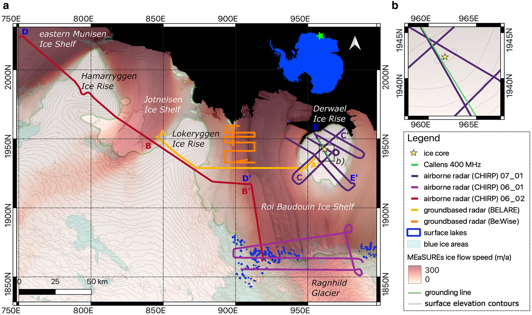
Figure 1. (a) Princess Ragnhild Coast with the location of airborne and ground-based radar profiles. MEaSUREs surface velocities (Rignot and others, Reference Rignot2019) and surface lakes (Stokes and others, Reference Stokes, Sanderson, Miles, Jamieson and Leeson2019) are shown for context. The inset (b) details the location of a relevant ice core and a previous radar survey (‘Callens 400 MHz’ from Callens and others, Reference Callens, Drews, Witrant, Philippe and Pattyn2016) used to date the IRHs in this study. Capital letters mark the start and end points of sections shown in Figures 2 and 6. Surface elevation contours are shown every 50 m. The coordinate system is EPSG:3031 – WGS 84/Antarctic Polar Stereographic (units are in km). See Table 1 for survey details of CHIRP, BELARE and Be:Wise.
Surface accumulation rates are orographically controlled in many places along the Dronning Maud Land coast where many small ice shelves are bounded by promontory-type ice rises. There, increased snow deposition is observed on the eastern slopes (facing the mean wind direction) of all ice rises (Lenaerts and others, Reference Lenaerts2014; Goel and others, Reference Goel, Brown and Matsuoka2017, Reference Goel, Martín and Matsuoka2018; Kausch and others, Reference Kausch2020; Pratap and others, Reference Pratap2022). Surface accumulation rates also vary across topographic incisions that correspond to ice-shelf channels (Drews and others, Reference Drews2020). Little temporal changes in surface accumulation rates have been inferred from IRHs over the last few decades (Callens and others, Reference Callens, Drews, Witrant, Philippe and Pattyn2016; Cavitte and others, Reference Cavitte2022), but ice core data on DIR suggest increasing accumulation rates over the second half of the 20th century (Philippe and others, Reference Philippe2016). Extensive surface melting and ponding have been observed close to the grounding line in the blue-ice area of western RBIS (Lenaerts and others, Reference Lenaerts2017) and JIS giving rise to several surface lakes that are also visible in satellite imagery (Stokes and others, Reference Stokes, Sanderson, Miles, Jamieson and Leeson2019). Their presence has been attributed to erosive katabatic winds blowing down from the ice sheet to the ice shelf where they expose blue ice which has a lower albedo and in turn absorbs more heat (Lenaerts and others, Reference Lenaerts2014). The RBIS receives little to no basal freeze-on (Berger and others, Reference Berger, Drews, Helm, Sun and Pattyn2017) of marine ice (Tison and others, Reference Tison, Ronveaux and Lorrain1993; Jansen and others, Reference Jansen, Luckman, Kulessa, Holland and King2013; Koch and others, Reference Koch, Fitzsimons, Samyn and Tison2015). Instead, it experiences widespread moderate basal melting of a few meters per year (Pattyn and others, Reference Pattyn2012; Berger and others, Reference Berger, Drews, Helm, Sun and Pattyn2017; Sun and others, Reference Sun2019) and enhanced localised basal melting in ice-shelf channels (Drews and others, Reference Drews2017).
3. Methods
Changes in the density and ice crystal orientation influence dielectric permittivity and together with changes in conductivity are the major causes for radar reflections from within the ice forming IRHs (Fujita and others, Reference Fujita, Maeno and Matsuoka2006). In the well-stratified interior of the Antarctic Ice Sheet, long sections of IRHs are clearly visible in many radar datasets (Winter and others, Reference Winter, Steinhage, Creyts, Kleiner and Eisen2019; Cavitte and others, Reference Cavitte2021). In coastal areas, however, surface meltwater infiltration or ice-dynamic buckling and shearing can render this stratigraphy invisible to radar (e.g. Karlsson and others, Reference Karlsson, Rippin, Bingham and Vaughan2012) also leading to disrupted IRHs (Karlsson and others, Reference Karlsson, Rippin, Bingham and Vaughan2012; Keisling and others, Reference Keisling2014). In that sense also the absence of IRHs contains valuable information, although more difficult to interpret as no IRHs can also be a result of insufficient radar system sensitivity at larger depths and in regions of high englacial attenuation (Drews and others, Reference Drews2009).
Here, we have analysed data from two ground-based radar surveys with an airborne survey using the multichannel ultra-wideband (UWB) radar of the Alfred Wegener Institute (AWI) (Table 1). All three radar campaigns together cover three ice rises and large parts of the ice shelves in this region (Table 1; Fig. 1).

3.1 Collection and processing of (cross-platform) radar data
3.1.1 Airborne radar profiling
In austral summer 2018/19, AWI's airborne UWB radar (multichannel coherent radar depth sounder; MCoRDS5; Rodriguez-Morales and others, Reference Rodriguez-Morales2014; Hale and others, Reference Hale2016; Franke and others, Reference Franke2021) mounted on the Polar6 aircraft (Alfred-Wegener-Institut Helmholtz-Zentrum für Polar- und Meeresforschung, 2016) was used to acquire radar data over the area of interest (CHIRP campaign; Fig. 1, Table 1). The transmission signal is composed of three-staged linear modulated chirp signal (1 μs unamplified, 1 μs high-gain and 3 μs high-gain) operating at a frequency range of 150–520 MHz. The 1 μs low-gain waveform is used to detect the ice surface and to resolve layers in the upper ice column. The short transmit signal without amplification avoids clipping of the surface reflection and does not mask reflections in the firn column. Standard processing techniques using the CReSIS Toolbox (CReSIS, 2021) for pulse compression, synthetic aperture radar (SAR) focusing and array processing were performed (for further details on radar data acquisition and processing, see Rodriguez-Morales and others, Reference Rodriguez-Morales2014; Hale and others, Reference Hale2016; Franke and others, Reference Franke2022). Additionally, the data were SAR-processed with a wider angular range (Franke and others, Reference Franke2022), which improves the signal-to-noise ratio for steeply inclined IRHs. The final radar data product has a range resolution of ~0.35 m and an along-track trace spacing of ~6 m.
In the airborne radar dataset, the surface multiple (i.e. a multiple reflection between the plane and the surface), as well as multiple reflections of shallow IRHs appear at about 50% of the ice thickness (Figs 2b, c). These multiple internal reflections below the surface multiples are mostly so prominent that they strongly limit visibility of IRHs at the corresponding depth and make them undetectable (Fig. 8). Therefore, IRH analysis of the airborne dataset is restricted to depths above these surface multiples. The ice–bed and ice–ocean interfaces can always be unambiguously identified. Internal stratigraphy is clearly visible in the firn layer (Fig. 7), with an approximate layer resolution (here defined as the ability to distinguish between two horizons) of 1 m.
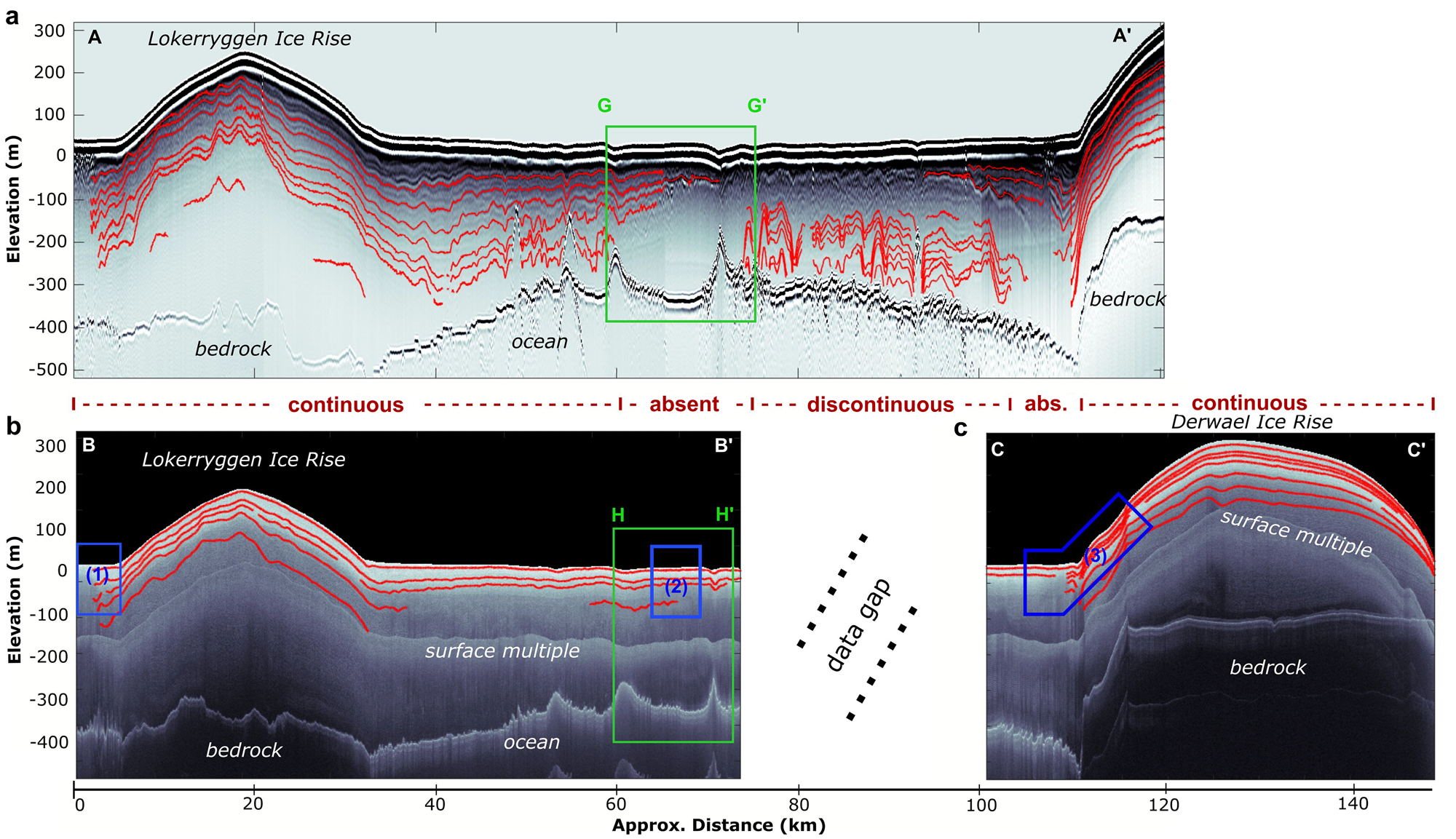
Figure 2. IRHs in two near-parallel radar profiles: low-frequency ground-based profile (A–A’) and UWB airborne CHIRP profile (B–B’ and C–C’). See Figure 1 for profile locations. Zones of predominant IRH types (continuous, discontinuous or absent/IRH-free zones) over depth are denoted for radar profiles above and below. Airborne data (B–B’ and C–C’) show a prominent surface multiple at mid-depth through the ice column (preventing any deeper detection of IRHs). Blue boxes indicate the location of pattern matching zones, shown in more detail in Figure 3. Green boxes denote the location of radar profiles highlighting IRH-free zones in G–G’ and H–H’ as shown in Figure 6.
3.1.2 Ground-based radar profiling
Ground-based radar data were acquired in 2010 (BELARE campaign) and 2012 (Be:Wise campaign) over the western RBIS (Fig. 1). These data were partly analysed in previous studies (Pattyn and others, Reference Pattyn2012; Drews, Reference Drews2015; Drews and others, Reference Drews2020), however, not in terms of assembling the IRH stratigraphy. BELARE and Be:Wise data were collected using a monopulsed transmitter and resistively loaded dipole antennas (Matsuoka and others, Reference Matsuoka, Pattyn, Callens and Conway2012) operating at frequencies 5 and 20 MHz, respectively (Table 1). The system was towed at an average speed of 10 km h−1, resulting in an average trace spacing of <10 m. The data were dewowed and bandpass filtered prior to IRH tracing. Higher frequency ground-based radar data also previously collected in this area are covered in a different study (Cavitte and others, Reference Cavitte2022).
3.2. Semi-automatic tracing of IRHs
We implemented a trace-by-trace IRH-tracking scheme that follows distinguishable maxima (or minima) within a window of similar travel time across traces and can be used with airborne and ground-based datasets. For the airborne data, seed points are initially calculated using a continuous wavelet transform (Xiong and others, Reference Xiong, Muller and Carretero2017) and then combined with the maximum/minimum tracking. More details of the layer tracing can be found in Appendix A.1. In some cases, pattern matching of characteristic layer packages across observational gaps/shear zones in a single dataset was possible (Fig. 3), and this information is tagged in the available IRH datafiles (Table 2).
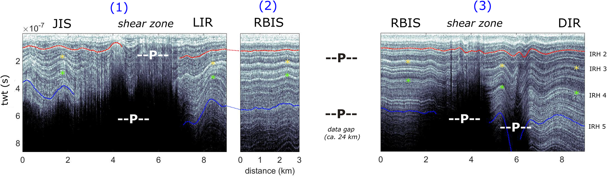
Figure 3. Pattern-matched IRHs 2 and 5 across two ice rises and two ice shelves (JIS, Jotneisen Ice Shelf; LIR, Lokeryggen Ice Rise; RBIS, Roi Baudouin Ice Shelf; DIR, Derwael Ice Rise). Pattern matching was necessary across two shear zones and one data gap of ~24 km. Layers identified and used to pattern match across the data gaps are denoted with stars (--P-- for pattern match).
Table 2. IRH datasets generated in this study with basic statistics of IRH packages

The airborne radar dataset was separated into two geographic regions: Daerwell (CHIRP: line 20190107_01) and all other ice rises and ice shelves in this region (CHIRP: line 20190106_02). All IRHs are available at PANGEA (Koch and others, Reference Koch2023a).
The travel time of IRHs was converted to depth using an empirical density–permittivity relationship (Kovacs and others, Reference Kovacs, Gow and Morey1995), and average depth–density profiles from two ice cores in our research area (Hubbard and others, Reference Hubbard2013; Philippe and others, Reference Philippe2016). Following suggestions of earlier studies (e.g. Rippin and others, Reference Rippin, Siegert, Bamber, Vaughan and Corr2006; Karlsson and others, Reference Karlsson, Rippin, Vaughan and Corr2009; Karlsson and others, Reference Karlsson, Rippin, Bingham and Vaughan2012), we classified zones with (1) well-preserved and laterally continuous IRHs that can be traced over several tens of kilometres, (2) discontinuous and buckled IRHs, where tracing across the whole radar profile is difficult, and (3) zones in which IRHs are absent. The top and lateral extent of a distinct elongated IRH-free zone was mapped out manually as well as the location of other near-surface IRH-free zones near ice rises.
3.3 Derivation of surface accumulation rates from shallow IRHs
We used a shallow (<20 m) and laterally continuous IRH from airborne data to estimate the spatial variability of surface accumulation rates (IRH 2 in airborne radar data, Figs 9, 10). Our approach followed those of many others (e.g. Eisen and others, Reference Eisen, Nixdorf, Wilhelms and Miller2004; Cavitte and others, Reference Cavitte2022; Pratap and others, Reference Pratap2022) assuming that IRH depth is proportional to the surface accumulation rates (i.e. the shallow layer approximation (SLA, Waddington and others, Reference Waddington, Neumann, Koutnik, Marshall and Morse2017)) and ice dynamic thinning (e.g. Theofilopoulos and Born, Reference Theofilopoulos and Born2023) is neglected. Although along-flow strain rates on ice shelves and ice rises in our research area are similar, the assumptions of the SLA are less well justified on ice shelves (1) because of the strong horizontal advection (spatially misplacing the SMB estimate) and (2) because of basal melting which, albeit to a lesser extent than the surface accumulation, also imprints on the vertical advection (Drews and others, Reference Drews2020). However, the relative magnitude of the spatial variability in surface accumulation that we infer can be retained in spite of these limitations.
To obtain an age estimate on the traced IRHs, we assumed a steady age–depth relationship at DIR and tied the age of the airborne IRHs of this study collected in 2019 to those derived from a ground-based 400 MHz radar survey conducted in 2012 (Callens and others, Reference Callens, Drews, Witrant, Philippe and Pattyn2016), which was dated using a directly adjacent ice core (Philippe and others, Reference Philippe2016). This approach is comparable to Ashmore and others (Reference Ashmore2020) who also tied newly traced IRHs to IRHs from a previous radar survey that was dated by an adjacent ice core. The age–depth scale was transferred individually at five cross-over points with the CHIRP survey. As the IRHs in the two surveys occur at different depths, we interpolated the age–depth scale between IRHs with a third-order polynomial (Fig. 4). IRHs 2, 3 and 4 of the airborne CHIRP data are dated like this with years before 2019 of 16.4 ± 0.6, 27.1 ± 0.8 and 40.3 ± 0.6, respectively.
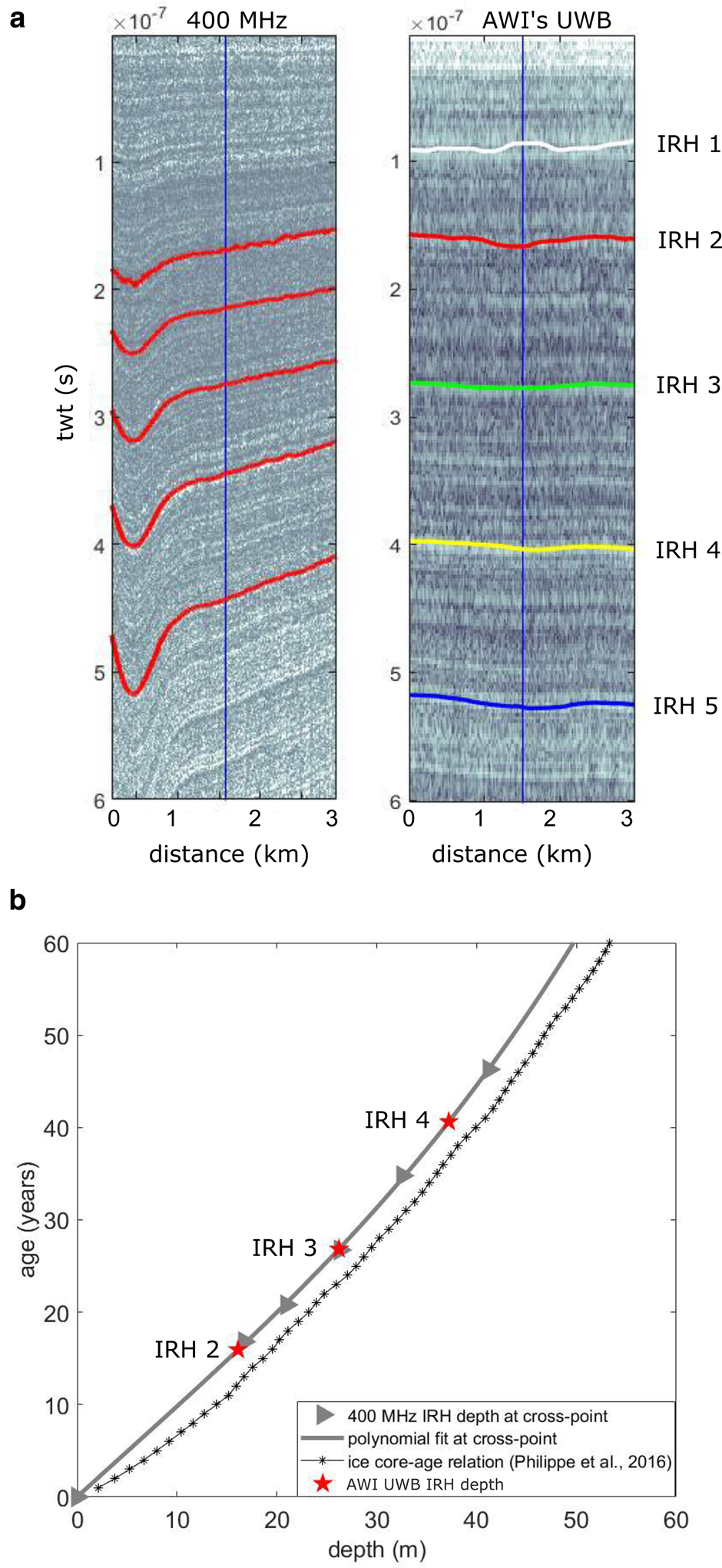
Figure 4. Dating of AWI UWB airborne radar-derived IRHs by linking with previously dated IRHs based on 400 MHz GPR profiles by Callens and others (Reference Callens, Drews, Witrant, Philippe and Pattyn2016) that extend to the ice core site. In (a) the original radar data and IRHs are shown with 400 MHz profiles on the left and the airborne radar profile (this paper) on the right. A blue vertical line denotes the crossing point of the two radar datasets. A third-order polynomial (forced through zero with zero depth equal to zero age) is fitted to the age–depth relationship at each cross-point site of both radar datasets. One age–depth relationship at one cross-point of the two radar datasets is displayed in (b) in comparison to the ice core depth–age relationship.
The IRHs were pattern-matched across data gaps by manually identifying distinct internal layer packages as in previous studies (e.g. MacGregor and others, Reference Matsuoka2015). For quality control, IRHs were visually matched across intersecting transects at cross-points and in closed loops when possible (e.g. Bodart and others, Reference Bodart2021; Cavitte and others, Reference Cavitte2022), such as at DIR. IRH2 was taken to derive past surface accumulation rates in the Princess Ragnhild Region since it is the IRH that allows the deepest almost continuous tracing in the area.
Uncertainties in the magnitude of surface accumulation rates result from the steady-state assumption between 2012 and 2019 (the years of the airborne and ground-based radar surveys), errors in the travel time-to-depth conversion (~0.25 m or 0.25 years at this depth), spatial variability in the depth–density profile, picking errors and uncertainties in the age–depth profile from the ice core itself (±1 year; Philippe and others, Reference Philippe2016). We accounted for this in bulk by assuming ±2 years in age uncertainty, and by calculating upper and lower estimates of surface accumulation rates in which all other factors reinforce each other (e.g. the lower estimate assumes an older, shallower IRH with a density profile resulting in less cumulative mass above the IRH). This resulted in a conservative error envelope for the inferred magnitudes (Fig. 5). The uncertainty of the surface accumulation rates can be reduced in future studies, e.g. by including an inverse-distance weighted average of the density profile from the various ice cores available in this area. Surface accumulation rates were additionally low-pass filtered with a cut-off period of 1 km to remove smaller-scale uncertainties that occur during picking. Even though the absolute uncertainties are large, the relative spatial variability of the accumulation signal can be interpreted across the whole dataset.

Figure 5. Average surface accumulation rates (from mind 2002 until the end of 2019) derived from IRH 2 of airborne radar data using the shallow layer approximation (SLA) (bottom) in comparison to RACMO surface accumulation from Lenaerts and others (Reference Lenaerts2013) (bottom) and topography (elevation and slope) (top). The shaded area in the lower plot includes the calculated error.
4. Results
4.1 Overview and characteristics of traced IRHs
We traced 77 IRHs with a total length of ~3700 km in the airborne datasets and ~2200 km in the ground-based datasets (Table 2). IRHs were traced continuously across individual segments and, when clearly visible, around bends in the radar transects. They are on average 190 km long in the airborne radar data and 25 or 62 km long in the ground-based radar data. In the airborne data, 24 IRHs were traced with the longest IRH as 314 km long (Figs 9, 10; Table 2). The shallowest IRH was traced at a minimum depth of a couple of metres below the surface and the deepest IRH was traced at a maximum depth of 222 m. At larger depths, the multiple reflection of the surface makes it more challenging to trace IRHs reliably (Fig. 8). In the ground-based data, 53 IRHs were traced at depths larger than 35 m and down to the ice–ocean interface (Figs 11, 12; Table 2). The maximal traced depth in these IRHs derived from the ground-based radar data is 416 m.
In general, continuous IRHs occur across all ice rises and also in large parts of the adjacent ice shelves, in particular when these are fed by the slower-moving ice from ice rises and the continental ice sheet (Fig. 1). Continuous IRH arches occur beneath ice divides of ice rises DIR (Figs 2c, 10), and near the saddles of HIR and LIR (Figs 2a, b, 9), likely as a combined result of the Raymond effect (Raymond, Reference Raymond1983) and local surface accumulation rate anomalies (Drews and others, Reference Drews2015; Kausch and others, Reference Kausch2020). The IRH arches will be considered in a different study constraining ice-rise evolution. Discontinuous or buckled IRHs were mostly detected at greater depths and predominantly in fast-flowing parts (Fig. 1) of shelf ice (below 100 m and extending to the ice–ocean interface whereby the lowermost IRHs are truncated, Figs 2a, 11, 12). IRH-free zones occur close to the grounding zones and in areas of horizontal shear.
In the grounding zones surrounding the ice rises, IRHs exhibit steep synclines resulting in IRH data gaps in numerous transects across ice rises into ice shelves (Figs 2a, b, c). These zones are typically subject to large gradients in ice surface flow velocities and associated with horizontal shear zones at the ice-shelf ice-rise transition (Fig. 6a). An exception is a transition from LIR into the RBIS where horizontal shearing is weaker (Figs 2a, b, 6). Two IRHs (IRH 2 and IRH 5) in airborne radar data were pattern-matched across two shear zones and a 24 km wide data gap based on the occurrence of characteristic layer packages (Fig. 3). While this approach increases uncertainties, it is currently the only way to transfer absolute accumulations rates from DIR to the other ice rises in the area (section 4.2). A localised IRH-free zone appears in all ground-based and airborne profiles at the RBIS (e.g. G–G’ in Fig. 2a) that are presented in section 4.3.

Figure 6. (a) Elongated IRH-free zone marked as green dots that also denote its top depth, derived from airborne and ground-based radar data. In addition, the transparent green circles denote locations of small IRH-free zones adjacent to ice rises. The locations of the ground-based (F–F’ and G–G’) and one airborne (H–H’) radargrams (as shown in b) are shown as yellow lines, overlain by the IRH-free depth markers on the map. Flowlines are shown as dotted positions for every 50 years. For context, surface ice-flow velocities are plotted in red, and horizontal shear strain rates in purple (Alley and others, Reference Alley2018) on the map. Panel (b) shows selected radargrams in which the IRH-free zone (that is marked in pink) is clearly visible. The ground-based radar data profiles F–F’ and G–G’ were filtered prior to analysis and the original amplitudes are thus not preserved. Therefore, the scale bar is left unitless.
4.2 Surface accumulation rates across ice shelves and ice rises
The longest traced continuous IRH (IRH2 in airborne radar data) connects all three ice rises in the near-surface in east–west oriented transects (D–D’ and E–E’, Fig. 1) over ~250 km (Fig. 5). Accumulation rates are lower on ice shelves than on ice rises and are higher on south-eastern (or windward) slopes (Fig. 5). Surface accumulation rates on ice shelves vary more strongly on sub-kilometre scales, particularly across surface depressions of ice-shelf channels (Fig. 5). The largest variability occurs across grounding lines and corresponding horizontal shear zones where characteristic synclines are most prominent (Figs 5, 6).
4.3 IRH-free zones
IRHs are absent in several areas: (1) in a distinct ~15 km-wide and ~100 m-thick laterally constrained elongated IRH-free zone or thick band that extends from the grounding line to the RBIS front to the west of the Ragnhild Glacier and (2) in the shear zones between the LIR and DIR and their adjacent ice shelves (Figs 2a, b, c, 6). The western limit of the IRH-free zone is defined with a comparatively abrupt transition from continuous IRHs to absent IRHs as visible in the ground-based data near the ice-shelf front (Fig. 2a, transect A–A’, box G–G’ and Fig. 6, transects F–F’ and G–G’). The eastern limit is more subtle and transitions across an ice-shelf channel east of which discontinuous IRHs emerge (Fig. 2a, transect A–A’, box G–G’). The ground-based radar profiles show a strong bright reflector above the elongated IRH-free zone (Fig. 6, transects F–F’ and G–G’). This zone is also detected in airborne profiles further upstream at shallower depths (Fig. 2b, transect B–B’, box H–H’ and Fig. 6, transect H–H’). Closer to the grounding zone, the lateral limits are more diffuse as IRH-free zones occur essentially across the entire ice shelf with a higher frequency to the west, where more surface lakes have been observed (Fig. 6a). The IRH-free zone progressively deepens downstream towards the ice-shelf front as continuous IRHs progressively develop near the surface from local snow accumulation (Lenaerts and others, Reference Lenaerts2017; Višnjević and others, Reference Višnjević2022). Consequently, the IRH-free zone, which forms a flow-parallel elongated band when connected in the across-flow radar profiles, is overlain by ~120 m continuous IRHs near the ice-shelf front (Fig. 6).
5. Discussion
5.1 Overview of IRH occurrence and contemporary ice dynamic setting
Occurrence of continuous IRHs, discontinuous IRHs or IRH-free zones generally coincides with respectively: (1) slow-flowing ice velocities over ice rises or within the top ten to hundreds of metres of ice shelves (Figs 1, 2) (IRH presence); (2) areas of fast ice flow such as the advected Ragnhild outlet glacier (Figs 1, 2) (IRH presence); and (3) areas of horizontal shearing (Fig. 6a) (IRH absence). In radar cross-section A–A’ in Figure 2, different ice bodies with continuous and discontinuous IRHs were classified and those zones are situated in slow and fast-flowing ice, respectively (Fig. 1). The link of IRH buckling to a fast-flow regime was observed in previous studies (e.g. Karlsson and others, Reference Karlsson2014; Ashmore and others, Reference Ashmore2020; Bodart and others, Reference Bodart2021). Since the undulated discontinuous IRHs occur at greater depth within RBIS (Fig. 2a), they have been advected from the land and subsequently further submerged because of continuing accumulation at the surface; such discontinuous IRHs have been previously associated with ice streams (e.g. Conway and others, Reference Conway2002). Once advected into the ice shelf, discontinuous IRHs were also further shaped by differential basal melting (Berger and others, Reference Berger, Drews, Helm, Sun and Pattyn2017) and by spatially variable surface accumulation rates (Drews and others, Reference Drews2020) considered in further detail in the following section. Increased localised basal melting also truncates IRHs (Figs 2a, 11, 12) at the ice-shelf base. This is most frequently observed at the basal incisions of ice-shelf channels within RBIS (Figs 11, 12). This strengthens previous assertions that basal melting can be heavily localised in ice-shelf channels (Marsh and others, Reference Marsh2016; Drews and others, Reference Drews2020; Schmidt and others, Reference Schmidt2023). While the processes for discontinuous IRH generation seem straightforward, we discuss further processes important for the development and interpretation of continuous IRH characteristics and those of IRH-free zones in the following two subsections.
5.2 Surface accumulation patterns over three ice rises and two ice shelves
Magnitudes and general patterns of the IRH-derived surface accumulation rates on RBIS (Fig. 5) compare in principle with atmospheric modelling results and previous observations. Increased orographic precipitation signatures on windward slopes with respect to mean wind direction are visible at the two eastern ice rises (DIR and LIR) and to a lesser degree also at the most western HIR (Fig. 5). This is in line with results from atmospheric modelling (RACMO (Fig. 5); Lenaerts and others, Reference Lenaerts2013) and observations at the same sites (Drews and others, Reference Drews2015; Callens and others, Reference Callens, Drews, Witrant, Philippe and Pattyn2016; Cavitte and others, Reference Cavitte2022). However, RACMO overestimates precipitation on the windward and underestimates precipitation on the leeward sides of the ice rises (Fig. 5). Such discrepancies in observed and simulated precipitation patterns should be accounted for in 3D modelling attempts of DIR, but also highlight the importance to obtain such spatially extensive in situ observations on a local to regional scale. Independent of these spatial differences, the good match in magnitude with previous observations and modelling results corroborates the accuracy of the dating and pattern matching approaches employed in this study.
Even though atmospheric modelling predicts spatially homogeneous surface accumulation rates over ice shelves (Lenaerts and others, Reference Lenaerts2014), IRH-derived accumulation rates show variability on spatial scales of less than about 3 km (Fig. 5). For example, surface depressions that occur near ice-shelf channels show signatures of wind erosion and re-deposition that have been observed previously in the Be:Wise dataset (Drews and others, Reference Drews2020). Here, we observe these patterns on all three ice shelves, emphasising that surface accumulation changes with the surface gradient especially across ice-shelf channels (Fig. 5). This is in line with several previous studies which have established this link over a wide range of spatial scales (e.g. Black and Budd, Reference Black and Budd1964; Spikes and others, Reference Spikes, Hamilton, Arcone, Kaspari and Mayewski2004; Drews and others, Reference Drews, Martín, Steinhage and Eisen2013, Reference Drews2020; Goel and others, Reference Goel, Brown and Matsuoka2017; Van Liefferinge and others, Reference Van Liefferinge2021). Insufficient resolution of surface topography could therefore be the primary reason for the mismatch on small spatial scales between radar-based accumulation rates and regional high resolution as well as continental- and regional-scale surface accumulation products. The observed smaller-scale variability becomes relevant, for example, when deriving basal melt rates with mass conservation near ice-shelf channels (e.g. Berger and others, Reference Berger, Drews, Helm, Sun and Pattyn2017).
The largest oscillations in surface accumulation rates occur across the grounding zones between ice rises and adjacent ice shelves (Fig. 5). This variability coincides with a strong change in surface slope from the ice rise to the ice shelf (Fig. 5) as well as large horizontal shearing (Fig. 6a). Since the IRH2, from which accumulation rates were derived, is located at a depth that is within the upper 5% of the ice thickness where the SLA typically applies, it is indeed likely that variable snow deposition might be the primary cause. Nonetheless, the calculated accumulation signal may be overprinted by four other factors: (1) unaccounted strain-induced effects in firn densification (Riverman and others, Reference Riverman2019; Oraschewski and Grinsted, Reference Oraschewski and Grinsted2022) impacting the travel time to depth and hence snow water equivalent conversion, (2) increased basal melt rates at the grounding line (Pattyn and others, Reference Pattyn2012; Berger and others, Reference Berger, Drews, Helm, Sun and Pattyn2017), (3) characteristic down warping of the IRH geometry (Figs 2b, c) as a result of persistent horizontal shearing (Hambrey and Lawson, Reference Hambrey and Lawson2000) (Fig. 6a) and (4) small vertical ice velocities that are inherent to ice dynamics across grounding zones (Lestringant, Reference Lestringant1994; Durand and others, Reference Durand, Gagliardini, de Fleurian, Zwinger and Le Meur2009). All these factors also increase the near-surface depression and hence contribute to increased topographically induced accumulation in the grounding zones. Disentangling all mechanisms would require a full-Stokes ice-flow model beyond the scope of this study. Nonetheless, the newly derived dataset of surface accumulation rates across three ice rises and two ice shelves now allows for catchment-wide accumulation assessment over the same time period.
5.3 Evidence for paleo-ice-stream activity advected into the ice shelf
The IRH-free zone or band of absent IRHs in the western part of the RBIS extends from the grounding zone to the ice-shelf front (Fig. 6a) as revealed by radar data presented in this study. Lenaerts and others (Reference Lenaerts2017) and Drews and others (Reference Drews2020) already detected the presence of an IRH-free zone in ground-based radar data near the ice-shelf grounding line but did not yet determine its full spatial extent toward the ice-shelf front, required to establish its origin. Here we discuss the possible physical processes that caused this elongated feature. We consider three main processes: internal lateral shearing, surface meltwater penetration and refreezing and blue-ice area advection. Given that this IRH-free zone or band is bound by continuous and discontinuous IRHs that were imaged much deeper on either side of the zone (e.g. Fig. 2a) by all radar systems, a lack of system sensitivity as an explanation can be excluded.
We suggest horizontal shearing as the primary cause for the existence of the IRH-free zone or band. Previous studies have found discontinuous IRHs or IRH-free zones to be associated with shear zones or basal ice deformation zones (Clarke and others, Reference Clarke, Liu, Lord and Bentley2000; Jacobel and others, Reference Jacobel, Scambos, Nereson and Raymond2000; Karlsson and others, Reference Karlsson, Rippin, Bingham and Vaughan2012; Holschuh and others, Reference Holschuh, Lilien and Christianson2019; Ross and others, Reference Ross, Corr and Siegert2020; Franke and others, Reference Franke2022). While persistent lateral shearing causes fold (syncline) formation (Jennings and Hambrey, Reference Jennings and Hambrey2021), IRH slopes progressively steepen with depth in RBIS similar to those created in land ice masses due to differential deformation (e.g. Hudleston and others, Reference Hudleston2015) until they cannot be imaged by radar anymore (Holschuh and others, Reference Holschuh, Christianson and Anandakrishnan2014). Small IRH-free zones occur together with such IRH synclines in our study area at the western limits of DIR where horizontal shear strain rates are highest within RBIS (Fig. 6a).
The syncline amplitude increases within the deeper IRHs (~15–50 m, Figs 2a, c) that have been exposed to strain for longer. However, these synclines of structural deformation origin are also influenced by increased local basal melting (Berger and others, Reference Berger, Drews, Helm, Sun and Pattyn2017) and spatially variable surface accumulation at this location (section 5.2). In the IRH-free elongated zone or band within the western part of RBIS, however, no shallow synclines are observed at the side of the zone, even though lateral shearing occurs, partially induced by (1) a pinning point located at the ice-shelf front (Berger and others, Reference Berger, Favier, Drews, Derwael and Pattyn2016) and (2) two ice masses of different origins and speed that merge as revealed by flowline tracing (Fig. 6a). The absence of synclines at the edges of the elongated IRH-free zone or band suggests that the horizontal strain rates within the ice shelf were not strong enough to visibly alter the continuous IRH geometry since deposition. This is corroborated by the presence of only slightly undulated continuous IRHs above and adjacent to the IRH-free zone (Fig. 6b, section G–G’). These continuous IRHs progressively developed downflow from the grounding line everywhere on the shelf towards the ice-shelf front, forming a local ice body of a maximum total depth of ~120 m (Višnjević and others, Reference Višnjević2022) (Fig. 6a). The interpretation of their localised formation downflow from the grounding line is consistent with the derived average surface accumulation rate of 300 kg m−2 a−1 over 400 years (advection time for shelf ice from the grounding line to the ice-shelf front using current flow speeds from Rignot and others, Reference Rignot2019), but it also matches the accumulation rates calculated from the SLA (section 4.2, Fig. 5).
A bright IRH (e.g. Dunmire and others, Reference Dunmire2020) at the top of the IRH-free zone (Fig. 6b) further supports this scenario, since it likely originates from refrozen surface meltwater from the grounding zone area where many surface lakes have been observed (Lenaerts and others, Reference Lenaerts2017; Stokes and others, Reference Stokes, Sanderson, Miles, Jamieson and Leeson2019). The reflector is slightly patchy (Supplementary Figs 3, 4, 7 and 11 in Drews and others, Reference Drews2020) in line with disconnected surface lakes. Since we present evidence that the relatively weak shear strain rates in the ice shelf were not strong enough to significantly alter the shape of IRHs since their formation at the grounding line, the IRH-free zone could constitute a remnant of a previous continental ice shear zone originating from the grounded shear zone of the Ragnhild glacier. Further corroborating the interpretation as a remnant and advected strain zone is that the location of the elongated IRH-free zone or band does not fully line up with today's surface strain field within the ice shelf. Most notably, it is offset by ~5 km eastwards in the Be:Wise data relative to the pinning point. Whether or not this signifies some temporal changes in the shear margin should be investigated in further studies which use this feature as a proxy for shear-margin migration over time.
There is weak evidence for an alternative explanation for the origin of the elongated IRH-free zone or band, i.e. that surface lakes have shaped this zone. It is not yet clear if surface meltwater infiltration and refreezing alone could also obscure deeper radio-stratigraphy, e.g. by disrupting the stratigraphy and creating a zone of warmer refrozen ice. It has been observed that ice-shelf surface lakes can drain abruptly (Banwell and others, Reference Banwell, Willis, Macdonald, Goodsell and MacAyeal2019; Dunmire and others, Reference Dunmire2020), and although direct evidence is yet missing, it appears that lake drainage is facilitated through vertical fractures into the deeper ice of the RBIS near its grounding line (Lenaerts and others, Reference Lenaerts2017; Dunmire and others, Reference Dunmire2020). Current flowlines at the eastern RBIS allow tracing back of the elongated IRH-free zone ice upstream into a grounded region that shows much blue ice and lakes (Fig. 6a). Whereas individual supra-glacial lakes at the grounding zone are only a few metres in water depth (Dunmire and others, Reference Dunmire2020), the elongated IRH-free zone within RBIS extends continuously to the ice-shelf base. Hence, the IRH-free band could be a temporally integrated signal of lake formation and near-surface refreezing. Hereby, slow ice advection over several hundred years, as flowline tracing upstream from the grounding line revealed, through an area of surface lakes before and after the grounding line (Stokes and others, Reference Stokes, Sanderson, Miles, Jamieson and Leeson2019) (Fig. 6a) could have contributed to shaping the zone. Especially if these surface lakes were topographically controlled by undulations in the underlying bed, with expression at the ice surface, they could have continuously formed in the same location. This would have created a refrozen lake upon a refrozen lake, stacked within the ice-shelf stratigraphy (and disturbing IRHs). However, this scenario is unlikely in shaping such a distinct elongated zone only, as lakes were extending across the whole ice-shelf grounding zone in recent satellite observations (Stokes and others, Reference Stokes, Sanderson, Miles, Jamieson and Leeson2019) and not just upstream of the elongated IRH-free zone. Hence this interpretation would be only plausible if surface lake presence and extent was a transient signal. It would require surface lakes at the grounding line to extend across almost the whole ice-shelf width having developed in recent years, whereas the lake presence upstream of the grounding line (in the blue-ice area) would have existed for several hundred or thousand years.
Another influence on the presence of the elongated IRH-free zone could be blue-ice areas that exist upstream of western RBIS next to Ragnhild Glacier (Fig. 1). Blue-ice areas have a negative (or zero) surface mass balance (Markov and others, Reference Markov2019) and the high local surface mass loss rates allow older and originally deeper ice stratigraphy to emerge at the surface (e.g. Koch and others, Reference Koch, Fitzsimons, Samyn and Tison2015; Baggenstos and others, Reference Baggenstos2018). According to the current flow field, the deeper continental ice at depth in western RBIS would have travelled through a blue-ice area for several thousand years. The localised surface ablation would result in deep ice layers coming to the surface that may not show continuous stratigraphy due to a previous intense deformation history of the deep ice on the continent.
Considering the ice dynamic context and the fact that the elongated IRH-free zone or band within RBIS has a very distinct lateral, longitudinal as well as vertical extent, we consider the interpretation as an advected remnant or paleo shear zone of the Ragnhild outlet glacier as the most likely one. This is more strongly backed up by the best observational evidence, even though this interpretation should be validated through modelling. Detailed stratigraphical investigations of ice shelves could hence also provide valuable information on the paleo strain history of the previous continental ice.
5.4 Scientific applications for mapped IRH stratigraphy in coastal regions
The IRH data presented in this study of the near-surface and internal ice stratigraphy allow for calibrations of as well as assimilation in ice-flow models applied to ice shelves and ice rises. For instance, Višnjević and others (Reference Višnjević2022) modelled the stratigraphy of the locally accumulated ice of RBIS, and validated results with the mapped shape and patterns of near-surface continuous IRHs from airborne radar (Koch and others, Reference Koch2023a). The mapped IRH stratigraphy could also be used to test whether or not the ice shelf has been in a steady state by comparing the observations with steady-state predictions of ice-flow models over the last hundreds of years (Višnjević and others, Reference Višnjević2022). Since the ice-shelf stratigraphy is affected by both surface accumulation and basal melting, it would now be feasible to use an inverse approach that distinguishes between these two factors incorporating deeper stratigraphy, such as discontinuous internal radar horizons. In terms of ice rises, our dataset fully unravels the 3D internal stratigraphy of DIR with a sufficient density that allows constraining 3D ice rise models (e.g. Pattyn and others, Reference Pattyn2012; Henry and others, Reference Henry, Drews, Schannwell and Višnjević2022). The mapped stratigraphy would help to constrain vertical velocities, which have thus far been derived through tuning snapshot inversions based on matching surface velocity observations to model output with varying basal slipperiness (Schannwell and others, Reference Schannwell2019, Reference Schroeder2020). With the full 3D stratigraphy, Raymond arches can be adequately represented which would also mean that vertical velocities would have been adequately modelled. The IRH stratigraphy that links HIR, LIR and – via pattern matching – DIR could also be used to study the coupled evolution of ice rises in neighbouring catchments. In addition, mapping and modelling the current and past locations of Raymond arches would also allow for the identification of the best suitable ice core-drilling locations (Steig and others, Reference Steig2006).
Shallow IRHs as well as those from deep within-ice shelves are also useful for improving (1) surface accumulation products and potentially (2) basal melt rate products that feed numerical simulations, allowing for more accurate ice dynamic reconstructions or predictions. Ice-shelf models are often fed by coarse input data of surface accumulation (e.g. RACMO; Lenaerts and others, Reference Lenaerts2014). The current accumulation rates derived from IRHs in this study could be used for bias correction, which is especially important since surface accumulation was established as the dominating forcing when modelling ice-shelf stratigraphy (Drews and others, Reference Drews2020; Theofilopoulos and Born, Reference Theofilopoulos and Born2023). In order to improve estimations of basal melt rates, traced synclines across grounding zones could be used to derive basal melt rates in combination with numerical simulations (e.g. Catania and others, Reference Catania, Conway, Raymond and Scambos2006; Pattyn and others, Reference Pattyn2012).
5.5 Need for standardised derivation and archiving of IRHs
We provide a stratigraphic dataset of IRHs derived from airborne as well as ground-based radar data, extending from the near-surface to the ice-shelf base and across ice rises and are hereby expanding IRH datasets in coastal areas of Antarctica. A few limitations of the IRH dataset presented here remain since few radar data have been collected along flowlines which is relevant for ice-shelf models (e.g. Višnjević and others, Reference Višnjević2022) and the 3D geometry of ice shelves is still not adequately sampled by radar transects presented here. We recommend (re)investigating ground-based radar data – when available – from previous field surveys together with airborne radar data in order to gain a comprehensive picture of the whole ice column or expand data coverage.
AWI's UWB airborne radar system (MCoRDS5) will be used for future efforts as part of the SCAR RINGS survey efforts albeit with a different flight altitude to avoid masking of the internal stratigraphy by a surface multiple. The system is capable of resolving IRHs in the firn with a resolution of about 1 m, as well as the entire deeper stratigraphy in similarly high resolution (Figs 2b, c, 7). Depending on the data acquisition set-up (e.g. platform, height above ground, transmit power, bandwidth, number of waveforms, waveform transmit time and gain) and the environmental conditions reflectivity at the ice surface and in the firn column, clipping can mask the upper IRHs. Our analysis found that AWI's UWB airborne radar system (MCoRDS5) is capable to detect the bed reflection as well as near-surface englacial reflections. This capacity gives a great opportunity to map both bed topography and SMB with a single survey flight. These two are major uncertainties when ice-sheet mass balance is determined using the input–output method (e.g. Bamber and others, Reference Bamber, Westaway, Marzeion and Wouters2018) and the primary targets of future RINGS surveys.
The derivation and archiving of IRHs from radar data is currently not a standardised procedure. While commercial and open-source seismic software are routinely applied to trace IRHs in radar data (e.g. Cavitte and others, Reference Cavitte2021, Reference Cavitte2022), these software mostly require a time-intensive manual tracing of IRHs. Hence, many IRHs have been traced by a wide variety of custom-programmed radar pickers with different semi-manual tracking schemes (e.g. Fahnestock and others, Reference Fahnestock, Abdalati, Luo and Gogineni2001; Mitchell and others, Reference Mitchell, Crandall, Fox and Paden2013; Panton, Reference Panton2014; MacGregor and others, Reference MacGregor2015; Xiong and others, Reference Xiong, Muller and Carretero2017; Delf and others, Reference Delf, Schroeder, Curtis, Giannopoulos and Bingham2020). Automating the detection of local maxima/minima of IRHs in backscattered power that occur at similar travel times in neighbouring traces often is a challenge and varies with the radar data type. Even when including layer slope (Panton, Reference Panton2014; MacGregor and others, Reference MacGregor2015; Delf and others, Reference Delf, Schroeder, Curtis, Giannopoulos and Bingham2020), most IRH tracing techniques operate only semi-automatically, i.e. require operator interference (e.g. MacGregor and others, Reference MacGregor2015; Xiong and others, Reference Xiong, Muller and Carretero2017). Our study used elements from previous studies (MacGregor and others, Reference MacGregor2015; Xiong and others, Reference Xiong, Muller and Carretero2017) to program ‘yet another picker’ to allow for IRH tracing in both airborne and ground-based radar data equally well (for more details on the picker see Appendix A.1.). This study provides no exception to the most common motivation for programming another tool: specific inputs/outputs were needed because of the radar platforms. Recent developments provide open-source radar processing software (e.g. Lilien and others, Reference Lilien, Hills, Driscol, Jacobel and Christianson2020), which could serve as a suitable platform for integrating the many available picking approaches. The classification of IRHs could also be included in future pickers since it would ease the interpretation of IRHs in relation to ice dynamics.
A larger-scale assembly of IRHs will be needed both for ice-sheet-wide model calibration and for developing more advanced IRH tracking methods to minimise operator interference in the future, such as deep learning to automatically track IRHs (e.g. Rahnemoonfar and others, Reference Rahnemoonfar, Yari, Paden, Koenig and Ibikunle2020; Varshney and others, Reference Varshney2021). Previous deep learning approaches rely on labelled datasets of IRHs for both training the network and evaluating its accuracy. Thus, the amount of available, labelled data currently limits the success of neural networks in identifying IRHs. While IRHs are increasingly becoming publicly available (Winter and others, Reference Winter, Steinhage, Creyts, Kleiner and Eisen2019; Ashmore and others, Reference Ashmore2020; Bodart and others, Reference Bodart2021; Cavitte and others, Reference Cavitte2021), a standardised community-wide process of data collection, processing and storing is required. We suggest saving IRHs together with metadata as outlined in Table 3. Here we include the date of the originally acquired radar profiles as well as their survey ID and profile ID, and the radar profile coordinates. For the IRHs, we include the dates of picking, the associated trace number, the two-way travel time of the picked IRHs (and optionally converted depth) and optionally the two-way travel time of the picked ice base (and optionally converted depth). Non-standardised data publishing currently makes it difficult to assemble IRHs generated by different institutions without relying on active submissions of individuals to community papers as was the case for radar-derived ice depth assembled for BedMachine (Morlighem and others, Reference Morlighem2017, Reference Morlighem2020; Frémand and others, Reference Frémand2023).
6. Conclusion
We mapped about 5900 km of IRHs semi-automatically in radar data of an ice-marginal Antarctic catchment. The analysed radar data were acquired in ground-based and airborne surveys between 2010 and 2019 over three ice rises and ice shelves in the Princess Ragnhild region. This study's focus was on characterizing the internal ice stratigraphy through mapping different types of IRHs that could (a) be used to derive spatially varying surface accumulation when dated (continuous IRHs) or (b) give information about elements of the ice-shelf deformation history (discontinuous IRHs or IRH-free zones) and ultimately provide an archive for calibrating and validating future modelling efforts.
Continuous IRHs in the Princess Ragnhild Coast region show increased accumulation on the eastern (windward) sides of topographic slopes as well as a strong small-scale variability across small-scale undulations within the ice shelf (like ice-shelf channels). While the large-scale trends for these orographic effects are known, our new data now correctly position surface accumulation maxima and minima in the respective flanks which is important for modelling ice-rise evolution. Linking three ice rises in this study via the interspersed ice shelves provides unique isochronal constraints that allow studying coupled ice rise evolution of neighbouring ice rises. Discontinuous IRHs mainly occur in deeper shelf ice that was advected from the dynamically active Ragnhild outlet glacier upstream. While discontinuous IRHs were associated with higher ice deformation previously, a discontinuous IRH dataset that extends all the way to the ice-shelf bottom allows the assessment of ice-shelf heterogeneity, which has implications for ice-flow modelling, hitherto rarely considered. The lack of IRHs in a spatially constrained elongated IRH-free zone within RBIS was interpreted as a proxy for the paleo activity of the shear margin with the Ragnhild outlet glacier. Checking other ice shelves for similar signatures could provide a valuable archive for ice-stream dynamics over the past hundreds of years.
The mapped internal ice stratigraphy of this study contributes to the ongoing mapping efforts of AntArchitecture and expands its focus toward the lesser-studied ice marginal zones. As the focus of airborne radar investigations shifts to the ice margins of Antarctica (Matsuoka and others, Reference Matsuoka, Forsberg, Ferraccioli, Moholdt and Morlighem2022), more data will become available. More and better observations of the ice-shelf stratigraphy allow – in combination with models – to distinguish steady-state ice-shelf dynamics from more recent transient responses. Accumulation patterns derived from IRHs could help validate surface accumulation products with which models are fed. Interpreted in combination with remotely sensed ice-flow dynamics or dated ice cores, IRHs also allow investigations into spatial variations or temporal stability (over several decades) of ice-shelf dynamics (processes).
Acknowledgements
Inka Koch, Reinhard Drews and Vjeran Višnjević were supported by an Emmy Noether Grant of the Deutsche Forschungsgemeinschaft (DR 822/3-1). Steven Franke and Daniela Jansen were funded by the Alfred Wegener Institute Strategy Fund, while Daniela Jansen was also funded by the Helmholtz Young investigator group HGF YIG VH-NG-802. Falk Oraschweski was supported by a scholarship of the ‘Studienstiftung des deutschen Volkes’. Logistical support was provided at Princess Elisabeth Station (Belgium), Troll Station (Norway) and Novolazarewskaja-Station (Russia). The airborne radar data were acquired in austral summer 2018/19 by the Alfred Wegener Institute, Helmholtz Centre for Polar and Marine Resarch (AWI) within the CHIRP project. We thank the Kenn Borek crew as well as Martin Gehrmann and Sebastian Spelz of AWI's technical staff of the research aircraft Polar 6. Furthermore, we thank John Paden, Tobias Binder and Veit Helm for their support regarding airborne data acquisition and processing. We acknowledge the use of the CReSIS toolbox from CReSIS generated with support from the University of Kansas, NASA Operation IceBridge grant NNX16AH54G and NSF grants ACI-1443054, OPP-1739003 and IIS-1838230. We thank Marie Cavitte and Nanna Karlsson for helpful discussions and tips around generating IRH datasets and Heiko Spiegel for picking IRHs at Derwael Ice Rise. In addition, we thank Joseph MacGregor and another anonymous reviewer for helpful comments that improved the clarity of the manuscript. Internal reflection horizons of this study are available on the PANGAEA data repository (Koch and others, Reference Koch2023a) at https://doi.org/10.1594/PANGAEA.950383. Radar data products from the standard work flow of the CHIRP survey are available on the PANGAEA data repository (Franke and others, Reference Franke2023) at https://doi.org/10.1594/PANGAEA.963264. Non-standard and raw radar data are available on request.
Author contributions
Inka Koch and Reinhard Drews designed the concept of the study. Reinhard Drews, Daniela Jansen, Olaf Eisen and Steven Franke planned the airborne radar survey and Daniela Jansen and Steven Franke collected the airborne radar data. Kenichi Matsuoka, Reinhard Drews, and Frank Pattyn collected the ground-based radar data. Reinhard Drews, Inka Koch and Vjeran Višnjević selected suitable data and – with input from Daniela Jansen – relevant topics for analysis/interpretation. Inka Koch, Reinhard Drews, Leah-Sophie Muhle and Falk Oraschewski developed the picker and picked the data. Inka Koch, Steven Franke and Leah-Sophie Muhle tagged the IRH data and finalised it. Inka Koch and Reinhard Drews drafted the initial manuscript, whereby all authors contributed to writing and editing. Inka Koch, Reinhard Drews and Steven Franke designed the figures of the manuscript.
Appendix
A.1. IRH picker
The IRH picker MATLAB code and supporting documents can be accessed on GitHub: https://github.com/Ice-Tub/picking_isochrones_v1/tree/paper. The picker requires that initial preprocessing of the radargrams has been completed so that the IRHs are clearly distinguishable. Some preprocessing is included as an option in the picker for the ground-based radar data to increase IRH visibility (e.g. bandpass filtering or Hilbert transformation). The picker is based on tracking a local maximum (or also local minimum for ground-based radar) of the received reflected power in an adjustable window across traces, corroborated by optionally employing a wavelet algorithm. Initially, the surface and basal reflectors are semi-automatically traced, applying standard maximum search techniques. The surface reflector is selected as the first largest peak, whereas the basal reflector is semi-automatically traced within a likely time interval defined by the user. Subsequently, the procedure of picking IRHs is different for airborne and ground-based radar data. For airborne radar data, significant wavelet peaks are identified in the whole radar dataset using Mexican Hat or Morlet Wavelets (Xiong and others, Reference Xiong, Muller and Carretero2017) and are marked as seed points. In order to calculate the seed points, the data below the basal reflector are considered background noise. Subsequently, the seed points are connected pixel by pixel laterally within a user-defined pixel time interval (‘a vertical window’) around each previously selected IRH pixel using a semi-automated search algorithm. Should no suitable seed points be available within the time window, the code selects the closest maxima instead. Depending on the nature of the specific IRH, this procedure can require a significant amount of user interaction wherever the automated tracing loses track of the corresponding IRH. Picking of IRHs in ground-based radar data relies solely on the semi-automated search for maxima/minima (and no seeds) due to the shape of the traces. Individual digitised IRHs in airborne or ground-based radar data can be connected between different profiles since cross-points are visibly marked in the picker to ensure internal consistency. In certain cases, this allows for checking of closed loops, a procedure often adopted for quality checking of picks (e.g. Winter and others, Reference Winter, Steinhage, Creyts, Kleiner and Eisen2019; Cavitte and others, Reference Cavitte2022). Surface and basal picks were corrected to the first break in the postprocessing. In addition to IRHs, the picker also allows basic picking of ice surface and base.
A.2. Explanatory note on the published internal reflection horizon data
The IRHs presented in this study are published in eight tab-delimited text files (see Table 2). For each of the four surveys (Belare 2010, Bewise 2012, CHIRP 20190602 and CHIRP 20190701; Figs 9–12) there is one file of IRHs in the twt domain and one in the depth domain, respectively. The locations of IRHs and the ice base are thus presented in seconds (twt) and metres (depth) with respect to the location of the ice surface. Note that the presentation of IRHs in Figures 9–12 is shown in elevation with respect to the REMA ice surface (Howat and others, Reference Howat, Porter, Smith, Noh and Morin2019). The column names, a description and the precision of the values are shown in Table 3. Non-data values are represented as ‘nan’. All IRHs have unique IDs within each survey (e.g. IRH_01 to IRH_29). Most IRHs are depth-sorted; however, in some cases, the IRH sequences are not unambiguous. Therefore, we highlighted in Figures 9–12 and in the file headers, which IRHs are depth-sorted and which are individual. The IRHs of the BELARE 2010 survey are depth-sorted, but divided into three individual sets (IRH_01-11, IRH_12-20 and IRH_21-29; see the three different colour codes in Fig. 11). The conversion from the twt domain to the depth domain includes a first-break correction and is based on the empirical density–permittivity relationship of Kovacs and others (Reference Kovacs, Gow and Morey1995) with averaged ice-core densities from Philippe and others (Reference Philippe2016) and Hubbard and others (Reference Hubbard2013).
The IRH data are published as tab-delimited text files and are stored in a PANGAEA publication series with a collective DOI (Koch and others, Reference Koch2023a)and four individual DOIs (Koch and others, Reference Koch2023b, Reference Koch2023c, Reference Koch2023d, Reference Koch2023e) for the respective datasets. The twt-based IRHs can be obtained from the ‘Source datasets’ section and the twt-derived depth-based IRHs from the ‘Other version’ section. An explanation for the column field names is presented in Table 3. In addition, figures of the IRHs in the elevation domain (Figs 9–12) for each dataset are archived under ‘Further details’. Note that the primary data (the twt-based IRHs) imported into the internal PANGAEA system have a more complex field notation according to the PANGAEA standards. This also affects the downloadable tab files, which have a different field structure than the one in Table 3. However, this field structure is explained on the respective dataset page in the ‘Parameter’ section.
Table 3. Explanatory notes for the columns in the internal reflection horizon (IRH) data files. Note that the information is valid for both, ‘twt’ and ‘depth’ files except for the ‘base’ and ‘IRH_N*’ columns


Figure 7. Representation of englacial layering in the airborne CHIRP radar profile 20190107_01_006 over Darwael Ice Rise with the AWI UWB MCoRDS5 system. (a) Radargram with the two-way traveltime (TWT) as recorded at acquisition (TWT between target and receiver) and (b) with the TWT from the ice surface reflection (i.e. flattened). The approximate depth scale of the entire ice column in (b) is 85 m.

Figure 8. Illustration of the effect of multiple reflections on englacial IRHs from AWI UWB profile 20190107_01_006 (panel a). Panels (b)–(f) show different magnified sections in which it becomes clear that: (i) the reflections on 50% of the ice thickness are indeed multiple reflections from internal layers below the surface reflections (panels c and d), (ii) partly only the surface multiples are visible and partly the surface multiples overprint the englacial IRHs (panel d), and (iii) both reflections are visible at the same time (panels e and f).
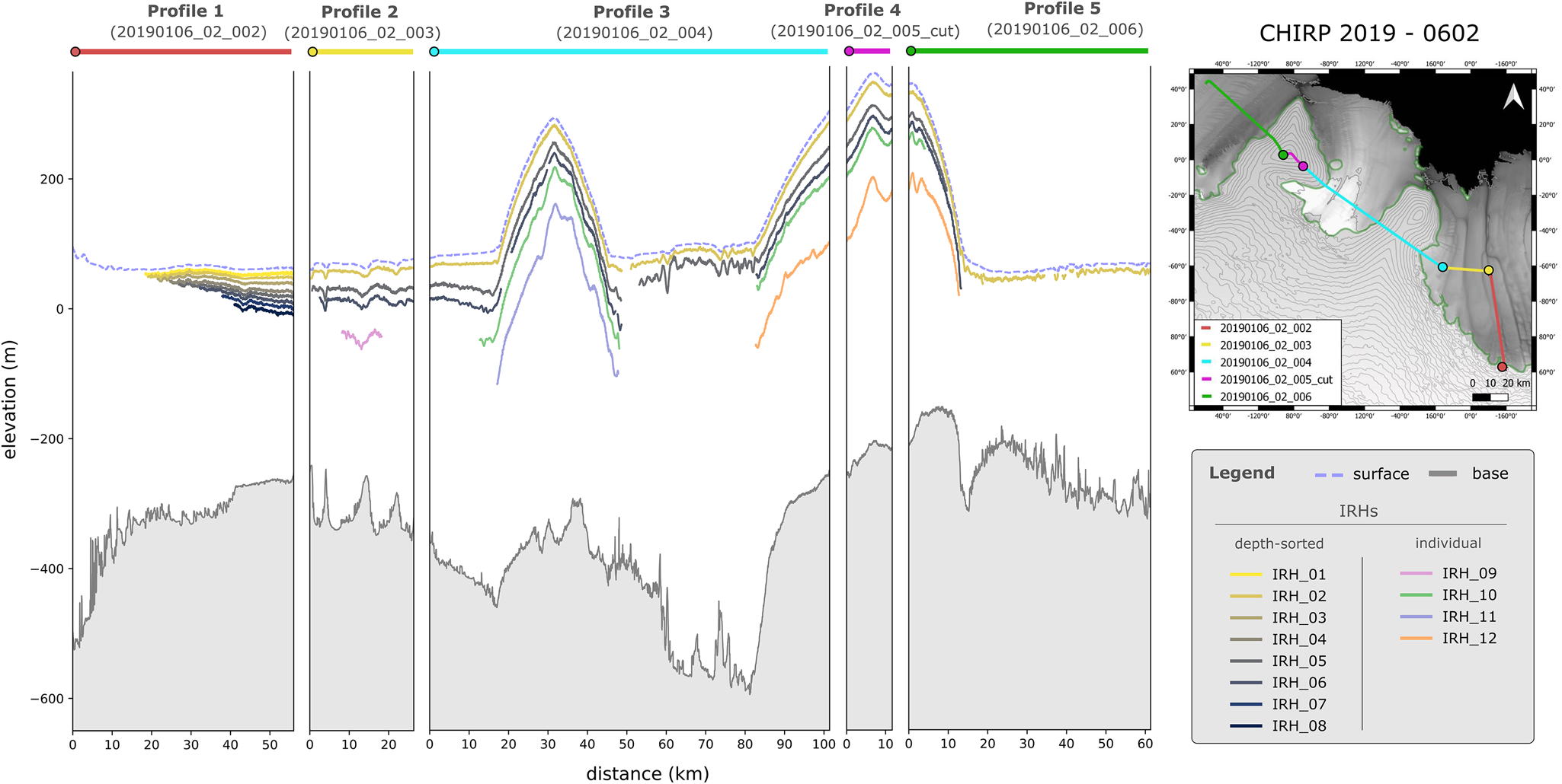
Figure 9. Representation of all IRHs and bed picks of the airborne CHIRP 2019 (0602) radar profiles in the elevation domain. Elevations were calculated using the REMA surface elevation model (Howat and others, Reference Howat, Porter, Smith, Noh and Morin2019). The positions of the profiles are marked by the respective colour in the upper right corner of the map. The circle always represents the starting point of the profile. The original name of the radar profile is shown on the top of each profile.

Figure 10. Representation of all IRHs and bed picks of the airborne CHIRP 2019 (0701) radar profiles in the elevation domain. Elevations were calculated using the REMA surface elevation model (Howat and others, Reference Howat, Porter, Smith, Noh and Morin2019). The positions of the profiles are marked by the respective colour in the upper right corner of the map. The circles represent the starting point of the profile. The original name of the radar profile is shown on the top of each profile.

Figure 11. Representation of all IRHs and bed picks of the ground-based BELARE 2010 radar profiles in the elevation domain. Elevations were calculated using the REMA surface elevation model (Howat and others, Reference Howat, Porter, Smith, Noh and Morin2019). The positions of the profiles are marked by the respective colour in the upper right corner of the map. The circle always represents the starting point of the profile. The original name of the radar profile is shown on the top of each profile.

Figure 12. Representation of all IRHs and bed picks of the ground-based Bewise 2012 radar profiles in the elevation domain. Elevations were calculated using the REMA surface elevation model (Howat and others, Reference Howat, Porter, Smith, Noh and Morin2019). The positions of the profiles are marked by the respective colour in the upper right corner of the map. The circle always represents the starting point of the profile. The original name of the radar profile is shown on the top of each profile.


 Open access