


1. Introduction
Investigating the structure of polar firn is important for understanding the response of glaciers and ice sheets to a warming climate. Modelling firn density is necessary for calculating ice sheet mass balance from altimetry measurements (Wingham, Reference Wingham2000; Alley and others, Reference Alley, Spencer and Anandakrishnan2007). The mechanical properties of firn are key to understanding processes of crevasse formation (Rist and others, Reference Rist1996), and potentially have implications for ice shelf rifting and hydrofracture (Kuipers Munneke and others, Reference Kuipers Munneke, Ligtenberg, Van Den Broeke and Vaughan2014; Hubbard and others, Reference Hubbard2016; Kulessa and others, Reference Kulessa2019).
Studying the structure of firn using seismic techniques requires wavelet velocities and amplitudes to be considered. Methods of measuring seismic velocity are well-developed: seismic velocity can be used as a proxy for density (Kohnen, Reference Kohnen1972) and can be used to estimate the thickness of the firn column (e.g. Hollmann and others, Reference Hollmann, Treverrow, Peters, Reading and Kulessa2021). Combined estimates of compressional (P) and shear (S) wave velocities can also be used to evaluate mechanical properties such as Poisson's ratio (King and Jarvis, Reference King and Jarvis2007) and elastic moduli (Schlegel and others, Reference Schlegel2019). In contrast, tools for quantifying attenuation, derived from amplitude losses, are less well developed. Attenuation is caused by both intrinsic mechanisms (elastic wave energy conversion) and apparent mechanisms (e.g. tuning and scattering); their combined effect is measured using the dimensionless seismic quality factor, or Q (O'Doherty and Anstey, Reference O'Doherty and Anstey1971; Schoenberger and Levin, Reference Schoenberger and Levin1974).
Measuring Q is desirable for two main reasons. The first is that correcting for attenuation through firn is an essential part of many glaciological measurements of seismic amplitude. These include amplitude-versus-offset measurements, which are important for identifying glacial substrates (e.g. Peters and others, Reference Peters, Anandakrishnan, Alley and Smith2007, Reference Peters2008; Booth and others, Reference Booth2012, Reference Booth, Emir and Diez2016; Horgan and others, Reference Horgan2021), as well as normal-incidence methods (e.g. Smith, Reference Smith1997; Muto and others, Reference Muto2019). However, current methods of measuring attenuation do not take into account the complex attenuative structure of firn, and often rely on the presence of multiple reflections, which are not always present with a sufficient signal-to-noise ratio (e.g. Dow and others, Reference Dow2013; Muto and others, Reference Muto2019).
Second, because Q is influenced by the physical properties of the propagating medium, measuring it has the potential to give further insight into the physical structure of firn. For example, the relationship between the compressional- and shear-wave quality factors and velocities in sands has been observed to be influenced by fluid saturation (Prasad and Meissner, Reference Prasad and Meissner1992), so measuring Q in firn may have implications for characterising firn hydrology. Recent observations of complex firn structure (Hollmann and others, Reference Hollmann, Treverrow, Peters, Reading and Kulessa2021) and large ice lenses within the firn column (Hubbard and others, Reference Hubbard2016) highlight the need for continued in-situ characterisation of firn and improvement of existing methods.
Although the continuous increase in seismic velocity with depth enables the velocity-depth structure to be measured in detail by relatively simple methods such as Wiechert–Herglotz inversion (Herglotz, Reference Herglotz1907; Wiechert, Reference Wiechert1910; Slichter, Reference Slichter1932), constraining the attenuation structure is less straightforward, due to the lack of convenient collinear raypaths. In this paper, we present a novel process of measuring the depth dependence of Q in the firn from diving waves (downgoing direct waves continuously refracted back towards the surface). We apply the process to data from Korff Ice Rise, West Antarctica, providing a more complete description of the firn's attenuative structure than has previously been possible. We complement these results with measurements made using primary and multiple reflections, their source ghosts, and direct waves, to validate the firn Q model and obtain a complete Q vs depth model for the entire glacier.
1.1. The seismic quality factor of snow, firn and ice
As a seismic wave propagates, it loses energy in three generic ways: geometric spreading, partial reflection at interfaces, and by conversion of kinetic energy to heat due to the internal friction of the propagating medium. The lattermost is termed seismic attenuation, and is quantified using a dimensionless quality factor Q. Q is proportional to the fractional energy loss per wave cycle (Aki and Richards, Reference Aki and Richards2002; Sheriff and Geldart, Reference Sheriff and Geldart1995), with higher Q materials associated with more efficient propagation. A wide range of P-wave quality factors (Q p) have been measured in both polar ice sheets and mountain glaciers; field-based measurements have ranged from Q p = 6 ± 1 in warm ice (Gusmeroli and others, Reference Gusmeroli2010), to Q p > 500 in cold polar ice (Bentley and Kohnen, Reference Bentley and Kohnen1976). A dependence of Q p on temperature has been demonstrated both in the laboratory (Kuroiwa, Reference Kuroiwa1964), and in the field (Peters and others, Reference Peters, Anandakrishnan, Alley and Voigt2012, using a method by Dasgupta and Clark, Reference Dasgupta and Clark1998). Clee and others (Reference Clee, Savage and Neave1969) measured both Q p and the shear-wave quality factor, Q s, in ice near its melting point.
Attenuation measurements have been made across various depth ranges, with some authors measuring Q over the entire ice column from the spectra of pairs of primary/multiple reflections (e.g. Robin, Reference Robin1958; Bentley, Reference Bentley1971; Jarvis and King, Reference Jarvis and King1993; Booth and others, Reference Booth2012). Others have measured Q within narrower depth ranges, either by using strong basal and englacial reflections (e.g. Jarvis and King, Reference Jarvis and King1993; Peters and others, Reference Peters, Anandakrishnan, Alley and Voigt2012) or by measuring the amplitude decay of the direct P wave in a vertical seismic profile (Booth and others, Reference Booth2020). Q has been measured in the uppermost ice of a snow-free glacier (Gusmeroli and others, Reference Gusmeroli2010), and at a single depth at the base of the firn column (Peters, Reference Peters2009); however little attention has been paid to the depth dependence of attenuation at intermediate depths in the firn column. Measurements of Q are therefore desirable to provide further insight into the structure of the firn itself.
In this study, we use continuously refracted seismic waves to measure the depth dependence of Q p in the firn column. We use measurements from basal reflection/source ghost pairs and critical refractions to corroborate our results. Q refers to the compressional-wave quality factor unless stated otherwise.
2. Data
2.1. Field site
Korff Ice Rise (KIR) is located in the Weddell Sea region of West Antarctica, surrounded by the Ronne Ice Shelf (Fig. 1). The ice is 530 ± 5 m thick at the divide (the boundary between ice flow directions), with flow velocity <10 m/a (Kingslake and others, Reference Kingslake, Martín, Arthern, Corr and King2016; Brisbourne and others, Reference Brisbourne2019). Seismic data were acquired in January 2015 along a line parallel to the ice divide.
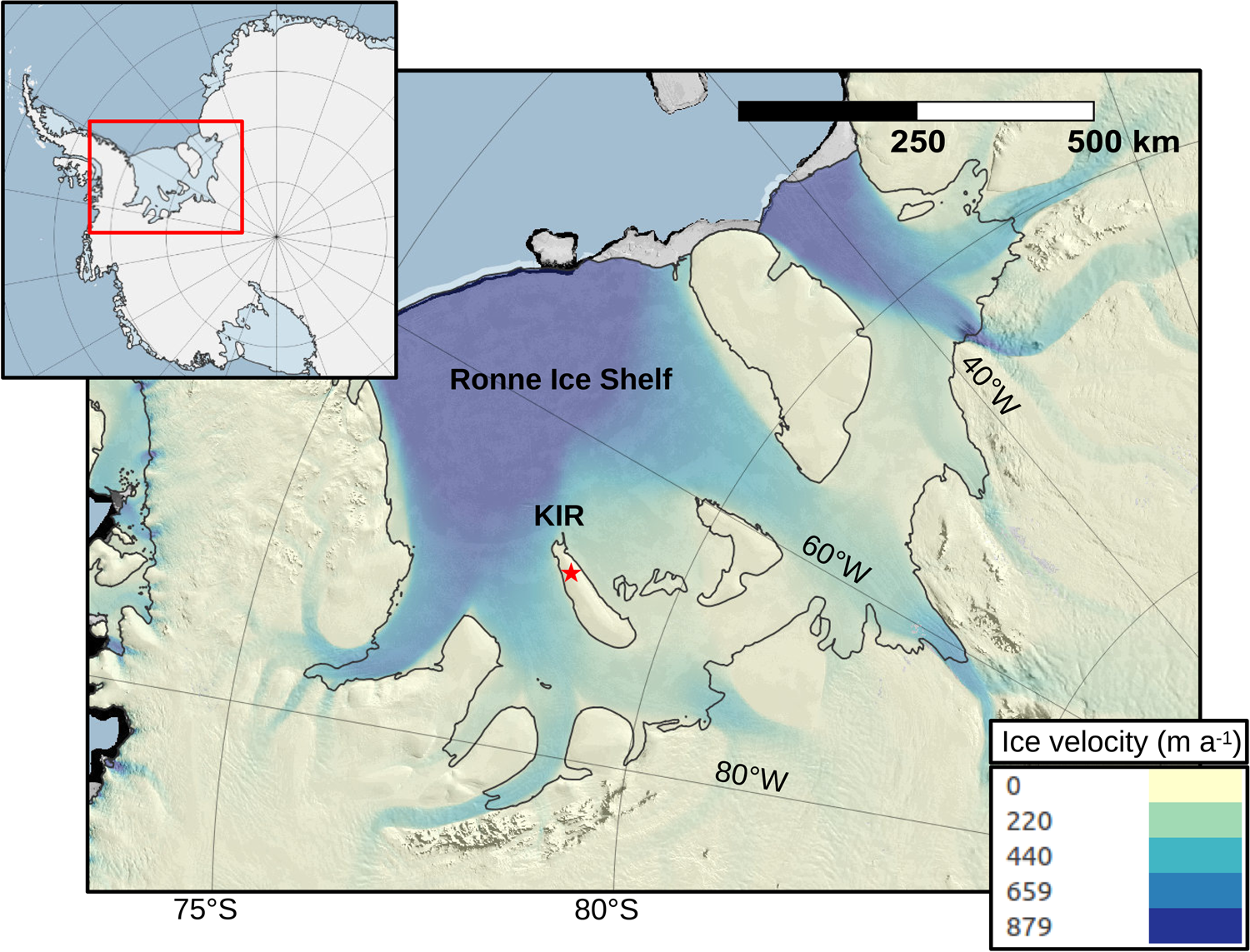
Figure 1. Location of the field site (red star) on Korff Ice Rise (KIR) in the Ronne Ice Shelf. Inset shows the location within Antarctica. MODIS imagery (Scambos and others, Reference Scambos, Haran, Fahnestock, Painter and Bohlander2007) is overlain by MEaSUREs flow velocities (Rignot and others, Reference Rignot, Mouginot and Scheuchl2011; Mouginot and others, Reference Mouginot, Scheuchl and Rignot2012, Reference Mouginot, Rignot, Scheuchl and Millan2017; Rignot and others, Reference Rignot, Mouginot and Scheuchl2017), accessed through Quantarctica (Matsuoka and others, Reference Matsuoka2021).
2.2. Surface-source data (acquisitions A1 and A2)
To constrain Q in the uppermost firn, a line of vertically oriented georods (Voigt and others, Reference Voigt, Peters and Anandakrishnan2013) was deployed with offset intervals progressively increased: 2.5 m between offsets of 2.5 m and 20 m, 5 m to 50 m and 10 m thereafter to a maximum offset of 390 m. A seismic detonator at the surface was used as the source. We call this acquisition A1; Data are shown in Figure 2a.
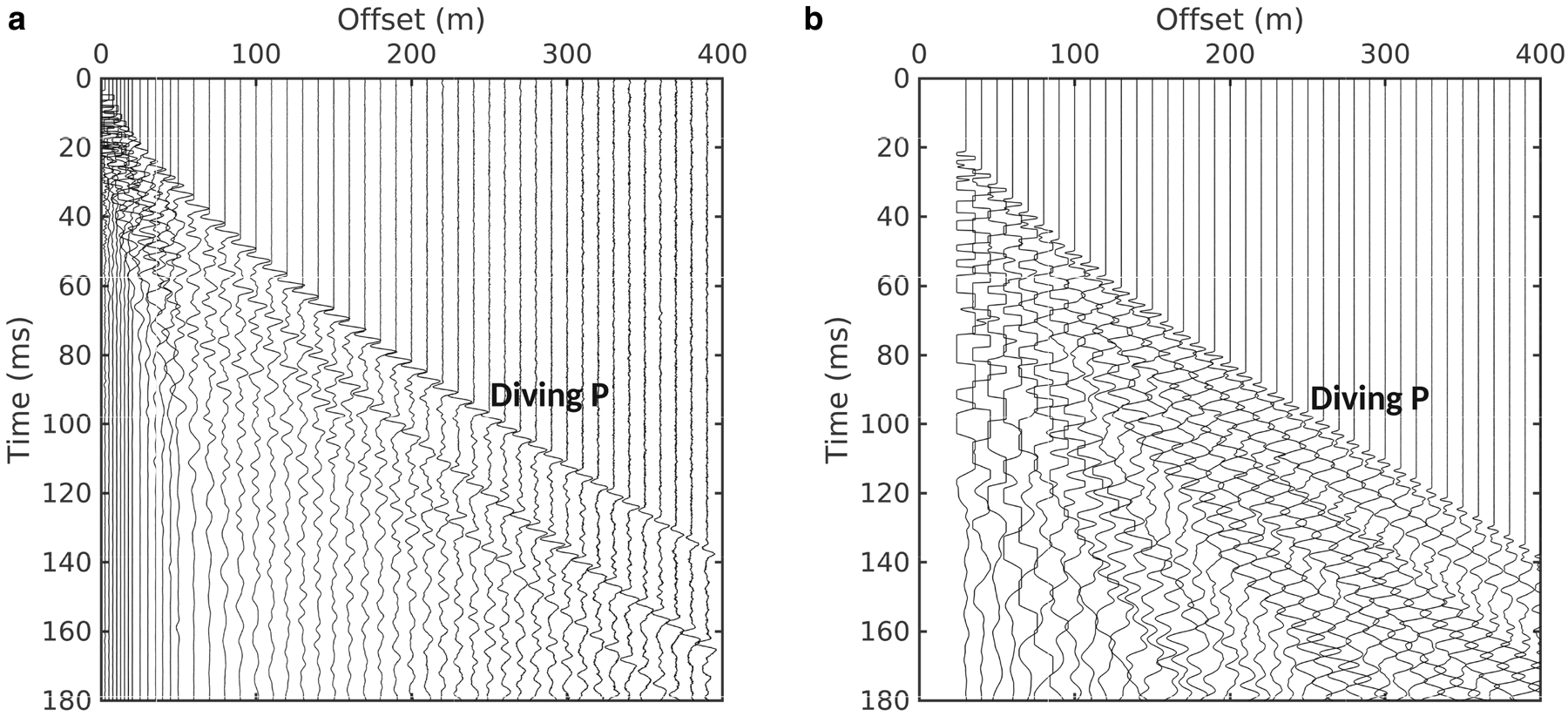
Figure 2. (a) Diving wave first breaks from the expanding spread refraction experiment (acquisition A1), used to constrain v and Q near the surface. Source: seismic detonator at surface. (b) First 400 m of diving wave first breaks from acquisition A2 used for the layer stripping computation. Source: 150 g Pentolite at surface. Traces are normalised in both (a) and (b).
To constrain Q deeper in the firn, we use data from a second acquisition, which we call A2: a line of vertically oriented georods, deployed at 10 m offset intervals between 30 m and 980 m. A 150 g Pentolite source was used, also at the surface, and 2 s of data were recorded with a 16 kHz sampling rate (data are shown in Fig. 2b).
2.3. Buried source data (acquisition B)
In addition to the layouts with the source at the surface, data were acquired from a line of vertically oriented georods at 10 m intervals, installed between 30 m and 1940 m offset, with a 150 g Pentolite source buried in a 20 m deep borehole. These data were recorded with an 8 kHz sampling rate. We call this acquisition B, and use these data to measure Q using the primary, multiple, source ghost and critical refraction. Figure 3 shows primary, source ghost and multiple phases.

Figure 3. Normal incidence traces from buried source data, acquired in acquisition B. (a) The primary reflection (PP) and its source ghost reflection (pPP) are used to measure Q above the source. (b) The primary and first multiple (PPPP) are used to measure Q from surface to bed. The source ghost (pPPPP) is also present.
A summary of acquisitions A1, A2 and B is given in Table 1. Data will be made available at the UK Polar Data Centre.
Table 1. Summary of acquisition geometries A1, A2 and B

3. Methods
The fundamental method we use is the spectral ratio method (Section 3.1), which we apply in different ways to measure Q in various portions of the ice column. The process we present to measure Q vs depth in the firn is layer stripping (Section 3.3). Layer stripping requires Q at the surface, Q 1, to be constrained independently, so we measure this using direct waves (Section 3.4.1), calling the result Q 1d. By initialising the layer stripping process with Q 1d, we obtain a full Q profile of the firn.
The other measurements we present corroborate our firn Q results. We measure Q from the surface to the bed, Q tot, using the primary reflection and first multiple (Section 3.2). By combining Q tot with our firn Q profile, we obtain Q in the section between the base of the firn and the bed, Q ice. We compare this to a measurement made in the uppermost solid ice from critically refracted waves, Q crit (Section 3.5). Additionally, we independently measure Q in the upper firn from the source ghosts of primary and first multiple phases, giving the results Q 1pg and Q 1mg (Section 3.4.2). We compare these to the direct wave result, Q 1d.
A summary of each measurement, its depth, acquisition type and offset range is given in Table 2; Figure 4 shows a schematic of the measurements and their depths.
Table 2. Summary of the survey layout used for each of the velocity and attenuation measurements


Figure 4. Schematic of measurements made and their depths. Note that depths are not to scale.
3.1. Spectral ratio method
Seismic attenuation is routinely measured using the spectral ratio method (Teng, Reference Teng1968; Båth, Reference Båth1974). The amplitude spectrum S(f, r) of a seismic wavelet of frequency f which has propagated a distance r with no transmission or reflection at interfaces is given by:

where S 0(f) is the initial spectrum, G(r) describes geometric spreading and a is the attenuation rate, related to Q by α = πf/Qv at frequency f and velocity v. The spectral ratio method compares the spectrum S A(f) of a reference wavelet A to that of a second wavelet B, S B(f), which travels for an additional time δt. The logarithmic ratio of the spectra is

Linear regression of the spectral ratio's logarithm against frequency allows a measurement of Q to be made from the slope m:

Figure 5 shows examples of wavelets, their spectra and associated logarithmic spectral ratios used for a calculation of Q in the firn (Section 3.3.1). In all spectral ratio measurements, a bandwidth must be chosen over which the spectral ratios are considered sufficiently linear; m is the curve's gradient within this bandwidth.
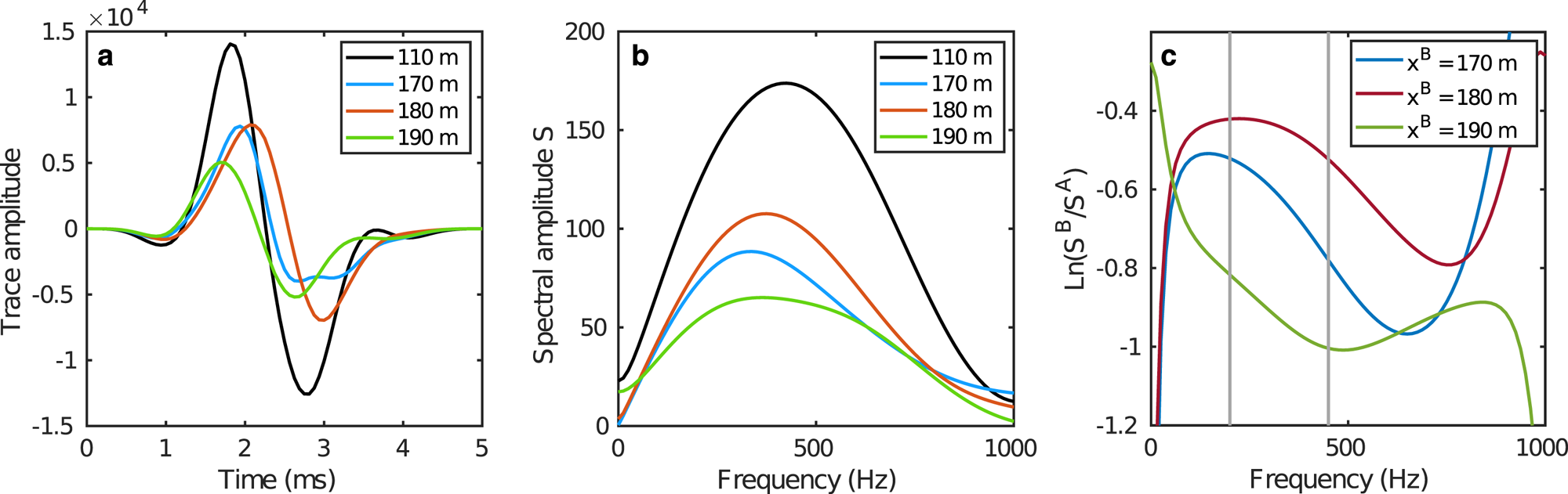
Figure 5. (a) Wavelets and (b) spectra of diving waves used for the calculation of Q in the second layer of the firn, Q 2. Legends (a) and (b) indicate the source-receiver offsets of the traces and spectra. The trace at 110 m offset (black) is used as the reference trace, with spectrum S A. (c) Logarithmic spectral ratios used for the calculation. The comparison trace has spectrum S B and source-receiver offset x B. The spectral ratios are considered to be sufficiently linear within the chosen bandwidth of 200 − 450 Hz, indicated by the grey vertical lines.
We use the common assumption that Q is independent of frequency (Kjartansson, Reference Kjartansson1979). We assume a low-loss formulation and definition of Q (e.g. O'Connell and Budiansky, Reference O'Connell and Budiansky1978; Toverud and Ursin, Reference Toverud and Ursin2005) and a non-dispersive velocity (Kjartansson, Reference Kjartansson1979; Liner, Reference Liner2012); we also assume that Q is isotropic.
Appendix B contains examples of traces, spectra and spectral ratios used for each application of the spectral ratio method.
3.2. Surface-to-bed Q measurement (Qtot)
A common process for measuring Q to correct for attenuation in seismic reflection studies is to use the spectral ratio of the primary reflection and its multiples (e.g. Booth and others, Reference Booth2012) with Equation (3). This gives the effective Q from surface to bed, Q tot, which includes the firn and its underlying ice (Fig. 6a). We select non-clipped normal incidence traces from acquisition B for our measurement (Fig. 3), taking incidence angles <10o as normal (Smith, Reference Smith2007). These wavelets and their spectra are shown in detail in Appendix B.
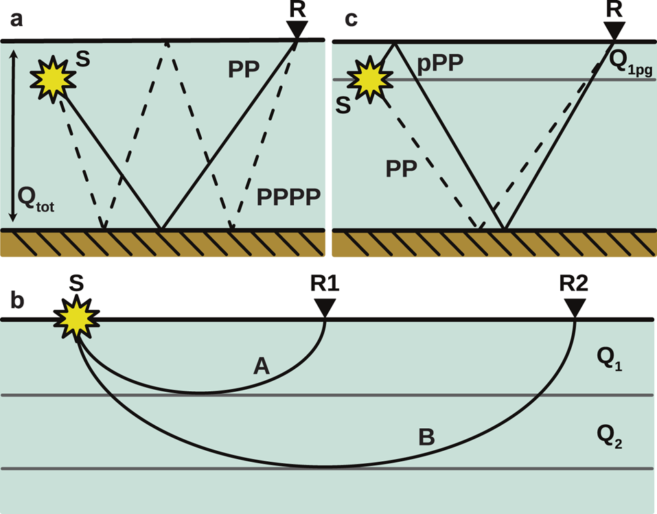
Figure 6. (a) The primary reflection (solid, PP) and first multiple (dashed, PPPP) are used to measure effective Q across the glacier's entire depth, Q tot. (b) Diving waves travelling between source S and receivers R1, R2. We define layers of constant Q and take the bottoming depth of the rays to be the layer boundaries. (c) The spectral ratio of the primary reflection (dotted, PP) and source ghost (solid, pPP) can be used to calculate Q in the uppermost layer, above a buried source. Note that this is schematic, and (a) and (c) do not show refraction of ray paths due to the firn's velocity gradient.
3.3. Deriving Q in the firn
The spectral ratio method usually measures the difference in frequency content of a propagating wavelet at different locations on an otherwise collinear path. We use a modified process which takes advantage of the firn's continuous velocity gradient and the resulting diving wave paths (e.g. Hepburn, Reference Hepburn2016; Alsuleiman, Reference Alsuleiman2018; Crane and others, Reference Crane, Lorenzo, Shen and White2018). We use Wiechert–Herglotz inversion to obtain a velocity model (WHI: Herglotz, Reference Herglotz1907; Wiechert, Reference Wiechert1910; Slichter, Reference Slichter1932); WHI has been widely used for application to firn (e.g. Kirchner and Bentley, Reference Kirchner and Bentley1990; Jarvis and King, Reference Jarvis and King1993; King and Jarvis, Reference King and Jarvis2007; Schlegel and others, Reference Schlegel2019; Hollmann and others, Reference Hollmann, Treverrow, Peters, Reading and Kulessa2021).
3.3.1. Layer stripping
For the purposes of this method, we represent the firn column as a sequence of layers of uniform Q; the stated quality factor for an individual quasi-layer describes the aggregated effect of attenuation over a defined vertical interval. Layer stripping is an established technique in seismic tomography and attenuation analysis (e.g. Quan and Harris, Reference Quan and Harris1997; Yilmaz, Reference Yilmaz2001), and it is the process by which we calculate the quality factor of an individual quasi-layer in the firn. This combines spectral ratio measurements of wavelets passing through that layer with an evaluation of the cumulative attenuation through all overlying layers.
Figure 6b shows two diving waves A and B arriving at receivers R1 and R2, having passed through different portions of the firn column. We trace these rays to find their depths of maximum penetration and interpret layers of uniform Q between these depths, discretising what we assume to be a gradual change in attenuative properties with depth as the firn compacts. The attenuated time t*, defined as t* = t/Q, is cumulative along each ray (Carpenter and others, Reference Carpenter, Bullard and Penney1966); i.e. for a ray which travels through n layers:

where t i is the time a ray spends in layer i, and Q i is the quality factor in that layer. A wavelet's attenuated time is not measured directly; however, the difference in t* between two wavelets, δt*, can be measured from their spectral ratio gradient m = −πδt*. Ray-tracing is used to determine the time each ray spends in each layer; combined with the measured spectral ratio gradients, this is used to calculate Q in each successive layer. Q n in layer n is calculated using the spectral ratio gradient of two rays A and B, which penetrate to the bottom of layers n − 1 and n, respectively:

Here, the superscripts denote the ray and the subscripts denote the layer; i.e., Q n is the quality factor in layer n, $t^A_i$ is the time ray A spends in layer i, and m B,A is the gradient of the spectral ratio S B(f)/S A(f). A derivation of this equation is given in Appendix A.
It is apparent from Equation (5) that the calculation of Q in each successive layer depends on the calculation of Q in all of the shallower layers. This process requires Q in the uppermost layer to be known before the others can be calculated; we measure this using near-offset direct waves (Section 3.4.1).
In principle, an attenuation-depth profile as smooth as the velocity-depth profile could be constructed using each successive offset pair; however, in practice, a vertical interval must be thick and/or attenuative enough that its Q contribution is detectable above noise. To obtain more robust results, we use clusters of three adjacent traces which, taken together, define the layer boundaries (Fig. 6b), calculating and averaging nine ${Q_i}^{-1}$ results for each layer. Figure 5 shows examples of traces, spectra and spectral ratios for the calculation of Q in the second layer. We choose traces and bandwidths based on inspection of individual spectra, avoiding traces with notched or unstable spectra.
We construct a four-layer Q p model based on available stable spectra with sufficiently large offset differences for a reliable measurement to be made, using data from the line of georods offset at 10 m intervals with a 150 g Pentolite source at the surface (acquisition A2).
3.3.2. Stochastic error analysis
We estimate uncertainties in velocities by applying Gaussian perturbations to wavelet travel times before Wiechert–Herglotz inversion, repeating the process to obtain distributions of velocities as a function of depth. We then calculate the mean and standard deviation of the output distributions to obtain velocity-depth curves.
To estimate the propagation of errors through the layer stripping process, we implement a stochastic framework of error analysis. After Q i is calculated for layer i, a Gaussian perturbation is applied to ${Q_i}^{-1}$ consistent with the uncertainty on the spectral ratio slope, and this perturbed Q i is used to calculate the Q i+1 of the next layer. We repeat this process 1000 times to obtain a large number of credible models to analyse statistically. In order to ensure that each generated Q(z) model is physically plausible, we assume two conditions and accept only models which satisfy these. We require that Q increases with depth (i.e., Q i+1 > Q i), and that Q > 0 always. We assume that the uncertainty is dominated by the spectral ratios and that the uncertainty from the travel-time measurement is comparatively small. Although these assumptions do not allow all theoretically possible results, we consider them necessary in order to obtain a large enough number of usable models from which statistics can be robustly calculated, given our computational constraints. All statistics are computed from distributions of the quantity ρ = Q −1, and results and uncertainties are quoted as the mean and standard deviation of the output distributions. The uncertainty in Q is then derived from $\epsilon _Q = \epsilon _\rho /\rho ^2$
 , where $\epsilon _Q$
 is the error in Q and $\epsilon _\rho$
 is the error in ρ (Topping, Reference Topping1972).
3.4. Constraining near-surface Q
Q(z) profiles output from layer stripping reveal relative variations, but evaluating absolute values requires Q in the shallowest layer, Q 1, to be constrained. We initialise our layer stripping process with a measurement of Q 1 from direct waves, which we call Q 1d, and use measurements from primary and multiple source ghosts (Q 1pg and Q 1mg) to support this result.
3.4.1. Direct wave measurement, Q1d
Measuring Q 1 from direct waves enables its constraint without the use of a buried source. Approximating near-offset diving waves as direct waves, we calculate Q 1d using their spectral ratios. The layer thickness d is the maximum thickness of the ray's first Fresnel volume, given by

where λ is the wavelength and x the source-receiver offset of the further offset ray in the pair (Spetzler and Snieder, Reference Spetzler and Snieder2004; Gusmeroli and others, Reference Gusmeroli2010). For the direct wave calculation, we use data acquired with a seismic detonator as source, which for our selected rays gives Q 1d in a layer 12 m thick. We initialise our layer stripping computation with Q 1d. For layer stripping, we use the nearest-offset non-clipped traces from acquisition A1; these rays reach 27 m depth, requiring that we assume Q 1 = Q 1d to 27 m.
3.4.2. Source ghost measurement, Q1pg, Q1mg
These results are used to corroborate the direct wave measurement of Q 1d. We acquired data with a buried source (20 m depth, acquisition B) which generates a discrete source ghost. We use these data to provide an independent measurement of Q in the upper 20 m. Figure 6c shows the ray paths of the primary reflection and its source ghost. The spectral ratio gradient for these two wavelets at normal incidence is used with Equation (3) to calculate Q, which we call Q 1pg. The traces used to calculate Q 1pg are shown in Figure 3a.
Shown in Figure 3b are the normal incidence first multiple (PPPP) and its source ghost (pPPPP). Measuring Q using these wavelets also gives Q in the firn above the shot, which we call Q 1mg. Ideally, we would expect Q 1pg and Q 1mg to be equal.
3.5. Constraining Q in the ice from multiples and critical refractions
3.5.1. Critical refraction, Qcrit
To validate the layer stripping approach to calculating Q, we make an independent measurement of Q in the uppermost solid ice, Q crit, using critically refracted waves (Peters, Reference Peters2009). Critical refractions occur at the point at which seismic velocity stops increasing. At this depth, Q crit can be straightforwardly measured using the spectral ratio of two critically refracted arrivals and Equation (3). For this measurement, we use data with a 150 g buried Pentolite shot (acquisition B). We calculate the thickness of this quasi-layer using Equation (6).
3.5.2. Combining Qtot with a firn-Q model
We combine our layer-stripping measurement with our measurement of Q tot to provide an estimate of Q between the base of the firn and the bed, Q ice:

Here, t ice is the travel time of a normal-incidence reflection between the base of the firn and the bed, t tot is the travel time between surface and bed, t i is the travel time in a layer i of the firn, and Q i is the quality factor of that layer. Since the measurement of Q ice is dependent on layer stripping, it is possible to validate the layer stripping process by evaluating the consistency of Q crit and Q ice.
4. Results
WHI yields the velocity-depth model shown in Figure 7a. The P-wave velocity increases with depth from 1200 ± 340 m s−1 at 1 m depth to 3779 ± 30 m s−1 at 90 m depth.
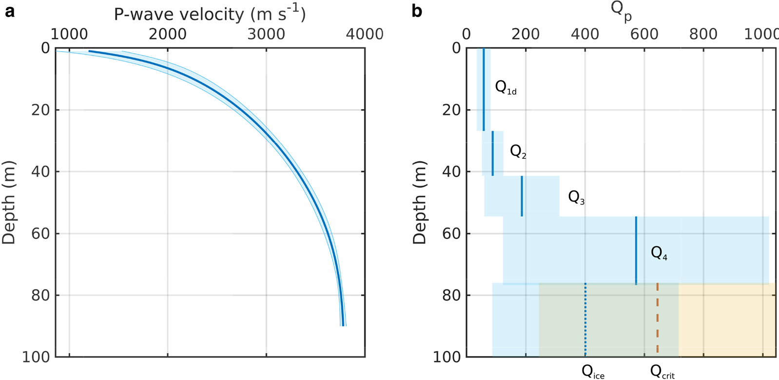
Figure 7. (a) Results from Wiechert–Herglotz inversion, showing the depth dependence of seismic velocity. (b) Dependence of quality factor Q on depth z. Q 1d is measured from direct waves and assumed constant to 27 m. Q 2 − Q 4 result from the layer stripping process. The blue dotted line shows Q ice resulting from combining the Q tot measurement with the layered model Q 1 − Q 4. The red dashed line shows Q at the base of the firn, Q crit, measured using the critical refraction. Shaded areas represent uncertainties.
The surface-to-bed Q is Q tot = 250 ± 100 measured using the primary and first multiple. The direct wave measurement of Q 1 gives Q 1d = 56 ± 23 in the uppermost 12 m of firn. From the primary reflection/ghost measurement, we find Q 1pg = 53 ± 20 for the uppermost 20 m, and from the first multiple/ghost, we find Q 1mg = 53 ± 24 for the uppermost 20 m.
The results of our layer stripping computation in combination with stochastic error analysis are shown in Figure 7b, which shows Q increasing to 570 ± 450 between 55 and 77 m depth. Table 3 presents the Q model resulting from the layer stripping process.
Table 3. Q p model from the layer stripping process, shown in Figure 7b

For the first layer, 0 − 27 m, we take Q 1 = Q 1d from the direct wave measurement.
By measuring Q at the critical refraction, we obtain Q = 640 ± 400 at 90 ± 14 m. This is indicated in Figure 7b by the dashed red line and shaded red area.
For a normal incidence reflection, our layered Q model, when combined with Q tot, implies that for the entire ice column at depths greater than 77 m, Q ice = 400 ± 310. This result is dependent on layer stripping and is shown in Figure 7b as the deepest layer with a dotted blue line, with errors indicated by the shaded area. Table 4 summarises all Q measurements which are independent of layer stripping.
Table 4. Summary of measurements independent of layer stripping

5. Discussion
We have shown an effective process of deriving the velocity and attenuation profiles through firn and ice, including a robust evaluation of uncertainties. Comparison of Q results obtained from layer stripping with independent measurements at similar depths shows consistency between methods. Our measurements of Q 4 = 570 ± 450, Q ice = 400 ± 310 and Q crit = 640 ± 400 agree with each other within uncertainties, supporting the use of the layer stripping process. The large uncertainties in our results arise from the variability in spectral ratio slope which propagates through the layer stripping process to Q 4 and Q ice. Furthermore, to conform with our stochastic error analysis, our quoted errors on Q are derived from the standard deviations of Q −1; other authors (e.g. Gusmeroli and others, Reference Gusmeroli2010) quote standard errors, which makes direct comparison inappropriate. Fundamentally, the uncertainties are determined by the bandwidth and signal-to-noise ratio of the diving-wave arrivals, which could be improved in many ways - for example, by ensuring excellent receiver coupling.
In the shallow firn, our measurements of Q 1d = 56 ± 23, Q 1pg = 53 ± 20, and Q 1mg = 53 ± 24 agree closely, despite the fact that the direct wave samples the top 12 m (Q 1d) and the source ghost samples the top 20 m of firn (Q 1pg, Q 1mg). This is suggestive of a shallow Q gradient in the upper firn.
A key motivation for measuring Q in the firn is the need to compensate for Q losses when the amplitude of seismic waves is of interest, for example when using amplitude-versus-offset (AVO) analysis to identify a subglacial material (e.g. Peters and others, Reference Peters2008; Booth and others, Reference Booth2012). We assess the impact of a layered Q model by considering what difference such a model would make to an AVO measurement versus a model which assumes a uniform Q tot throughout the whole glacier. We produce a synthetic AVO gather of a reflection from 530 m thick ice over bedrock, dominant frequency 200 Hz, which incorporates our detailed firn-Q model and velocity model. We then pick the amplitudes, and recalculate the bed reflection coefficient using (a) our detailed Q model including Q ice, and (b) the assumption that Q = 250 everywhere. We correct the amplitudes for a single frequency, f = 200 Hz. Figure 8a shows the two corrected reflectivity curves, and Figure 8b shows the percentage difference between the layered-Q corrected and uniform-Q corrected curves. The difference is small compared with typical signal-to-noise ratios at angles <50°, rising to $> 10\%$ at angles >50°. Layer stripping could therefore in theory provide a small benefit to AVO surveys which have very high-quality and wide-angle data. However, for typical glaciological AVO experiments layer-stripping will provide minimal benefits if Q can be measured using the primary and first multiple.
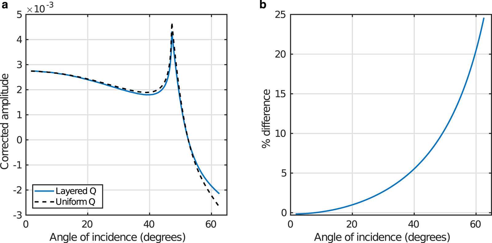
Figure 8. (a) Bed reflectivities obtained from synthetic amplitude-versus-offset (AVO) data simulating a reflection from an ice-bedrock interface with a Korff-like geometry, correcting for attenutation with a layered Q model (solid blue line), and a uniform-Q assumption (dashed black line). Data are not corrected for synthetic source amplitude and the y-axis is consequently multiplied by a constant. (b) Difference between layered-Q-corrected and uniform-Q-corrected AVO curves (%).
There are circumstances in which it would be preferable to choose a layer stripping measurement over a multiple-based one. First, for seismic experiments studying the firn itself, a measurement of Q in the firn is necessary, as clearly it is not valid to assume that Q at shallow depths is the same as the effective Q that would be measured using multiples. Second, thin layering at the ice-bed interface (Booth and others, Reference Booth2012) can cause interference effects which change the apparent amplitudes of the primaries and multiples, making a multiple-based measurement inappropriate where a thinly layered bed is suspected. Third, multiples are not always clearly visible in a seismic dataset (e.g. Dow and others, Reference Dow2013; Muto and others, Reference Muto2019); in such a case Q would need to be estimated by layer stripping.
Our method has potential for improvement. A more detailed model could be produced if more closely spaced, or even all, traces were used, resulting in a model with very thin layers and providing a more accurate representation of the continuous nature of firn transformation; however, this would require an extremely high signal-to-noise ratio that was not achieved with our dataset. In principle, layer stripping could be used to measure the shear-wave quality factor; the acquisition would need to be designed with this in mind, with an S-wave source and closely spaced receivers at near offsets. In addition to our P-wave data, we acquired S-wave data using a 600 g Pentolite source; however the size of the source needed to generate S-waves caused a high degree of clipping and contamination with P-waves, rendering a Q-analysis impossible. In the future, layer stripping could be combined with measurements relying on englacial reflections (e.g. Peters and others, Reference Peters, Anandakrishnan, Alley and Voigt2012) in order to build up a more comprehensive englacial Q-profile; this could be supplemented by a dedicated microspread to resolve detail at very shallow depths (e.g. Gusmeroli and others, Reference Gusmeroli2010). For complex firn structures such as those with ice lenses or hoar frost layers, WHI fails to capture the true velocity-depth relationship, and more advanced inversion methods such as full waveform inversion could be used to jointly invert for velocity and attenuation structures (e.g. Pearce and others, Reference Pearce2023a, Reference Pearce2023b).
6. Conclusions
We have demonstrated a novel application of the spectral ratio method for the measurement of the seismic quality factor Q in firn, and applied the method to data from Korff Ice Rise in West Antarctica. We have therefore been able to resolve the compressional-wave attenuative structure of firn in greater detail than has previously been possible. We have combined our layer stripping method with a stochastic method of error propagation. Our results show Q increasing from 56 ± 23 in the uppermost 12 m to 570 ± 450 between 55 and 77 m depth. We corroborate results from layer stripping with independent measurements using critically refracted waves, the source ghost and primary/multiple reflections. Using the primary reflection and source ghost shows Q = 53 ± 20 in the uppermost 20 m of firn, and using critically refracted waves shows Q = 640 ± 400 at 90 m depth. The layer stripping process can be used for seismic studies of firn or seismic reflection studies where conventional methods of measuring Q are not possible. Our results provide a fuller characterisation of firn's seismic properties than has previously been shown, and our methods will aid future seismic investigations of glaciological targets.
Acknowledgements
These data were collected as part of the British Antarctic Survey programme Polar Science for Planet Earth with the support of British Antarctic Survey Operations. RSA is supported by the NERC PANORAMA Doctoral Training Partnership. We thank the editor and three anonymous reviewers for their comments which greatly improved the quality of the paper.
Appendix A. Derivation
This is a derivation of Equation (5) seen in the main text. Here superscripts denote rays, and subscripts denote quasi-layers in the firn; e.g. $t^B_2$ is the time ray B spends in layer 2, and Q 2 is the quality factor in that layer. m B, A is the gradient obtained from the logarithm of the spectral ratio S B(f)/S B(A), where S B(f) is the spectrum of a wavelet following the path of ray B, and S A(f) is the spectrum of a wavelet following the path of ray A. Figure 6b shows two rays A and B, which reach the bottom of firn quasi-layers 1 and 2, with quality factors Q 1 and Q 2, respectively. These rays would be used to calculate Q in the interval between their maximum penetration depths, i.e. Q 2. The difference in their attenuated times is:

Assuming Q 1 is known, rearranging for Q 2 gives:

where δt*B,A is computed from the spectral ratio gradient m = −πδt*. Consider a ray C which penetrates to the base of a third layer; by a similar argument,

To calculate Q n in an arbitrary layer n, we would use the spectral ratio gradient calculated from two rays X and Y, one of which (Y) has penetrated to the base of layer n, and one of which (X) has penetrated to the base of layer n − 1. By extension of Equation (A.3), Q n is:

Appendix B. Data examples
Here we show examples of the wavelets, spectral amplitudes and spectral ratios relied upon for each of our measurements. In each figure, the legend indicates the source-receiver offsets of the traces used. In spectral ratio plots, the vertical grey lines indicate the bandwidth over which the gradient is measured. Figure 9 shows the relevant wavelets for the measurement of Q 1d in the top layer 12 m thick. Figure 10 shows the wavelets and associated spectra for the critical refraction measurement, for Q crit at the base of the firn column. An independent measurement of Q near the surface, Q 1pg was made using the primary reflection, PP, and its source ghost, pPP. Figure 11 (panels a-d) shows these wavelets and their spectra, and Figure 12a shows the associated spectral ratios, along with the bandwidth of measurement. A measurement was also made over the entire ice column of Q tot, using the primary and its first multiple (PPPP). These wavelets and spectra are shown in Figure 11 (panels e and f), with associated spectral ratios in Figure 12b. Finally, a third measurement was made of Q close to the surface, Q 1mg, from the first multiple and its ghost, pPPPP. Figure 13 shows these wavelets, their spectra and associated spectral ratios. Table 5 shows the bandwidth used for each measurement.
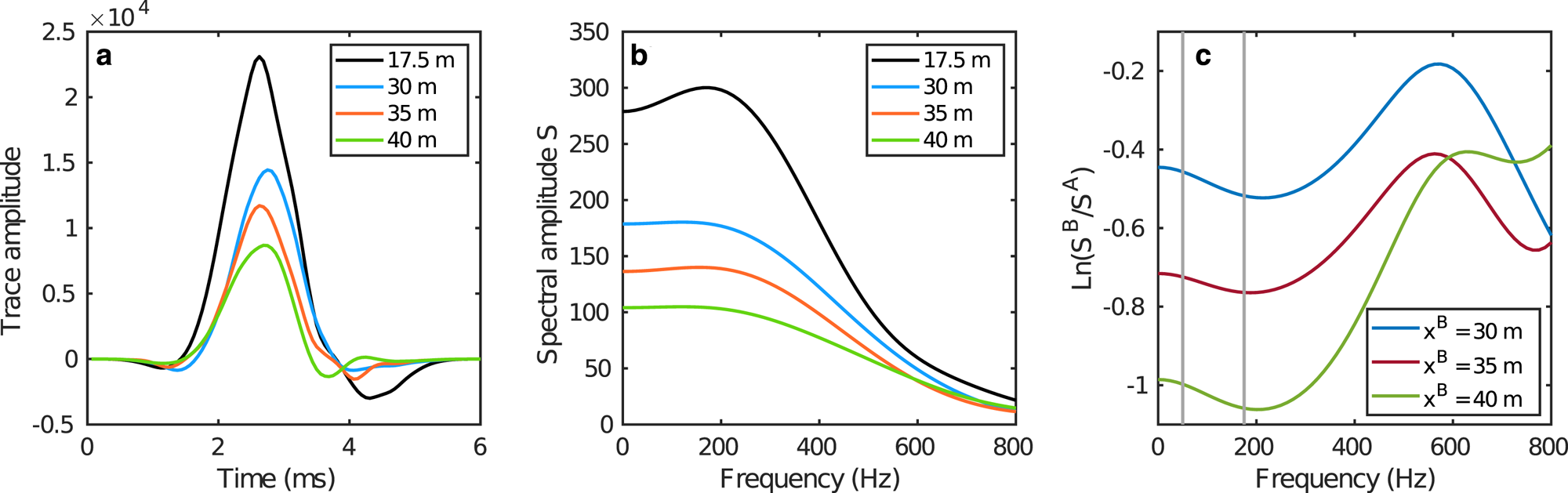
Figure 9. (a) Wavelets, (b) spectra and (c) logarithmic spectral ratios of diving waves used for the calculation of Q 1d in the uppermost layer (12 m thick). The spectral ratios are approximately linear within the chosen bandwidth of 50 − 175 Hz, indicated in (c) by the grey vertical lines. The legends in a) and b) indicate source-receiver offsets of traces and their associated spectra. In (c), S A is always the spectrum of the reference trace, at 17.5 m offset. x B is the source-receiver offset of the comparison trace, with spectrum S B, used to obtain the spectral ratio.
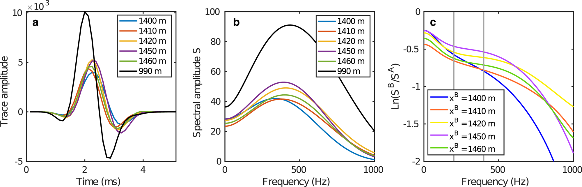
Figure 10. (a) Wavelets, (b) spectra and (c) logarithmic spectral ratios of critically refracted waves used for the calculation of Q at the base of the firn column, Q crit. Legends (a) and (b) indicate source-receiver offsets of traces. The reference trace, which has spectrum S A, is at 990 m offset. Legend (c) refers to the source-receiver offset of the comparison trace, x B, used to obtain the spectral ratio. The grey bars in (c) show the bandwidth of spectral ratio measurement, 200 − 400 Hz.
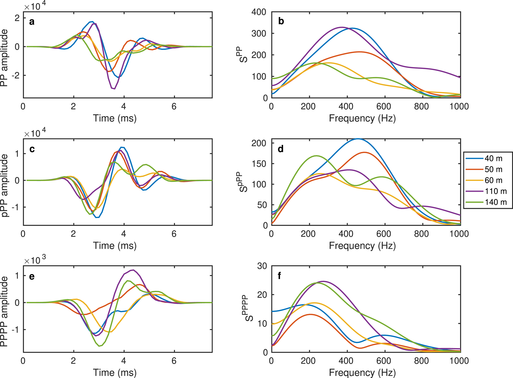
Figure 11. Wavelets and spectra recorded from buried-shot data. Primary reflection PP (a, b), its ghost pPP (c, d), and its first multiple PPPP (e, f).
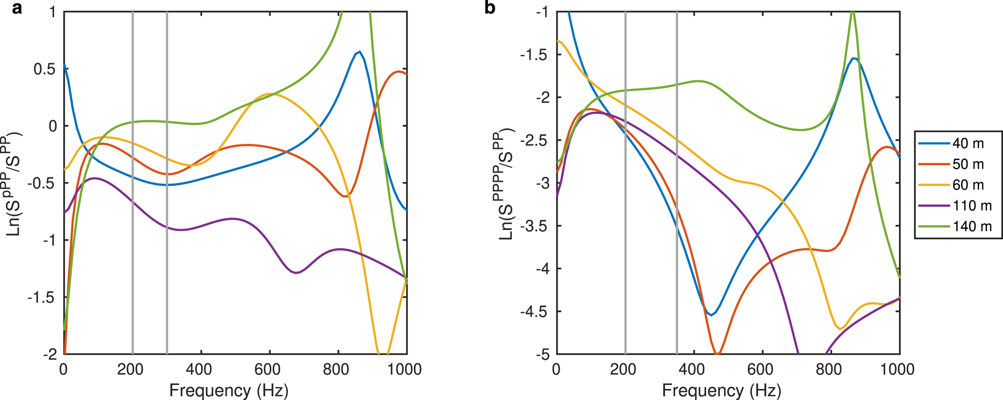
Figure 12. (a) Logarithmic spectral ratios of the primary and its ghost (pPP), used for the calculation of Q 1pg. (b) Logarithmic spectral ratios of the primary (PP) and first multiple reflections (PPPP), used for the calculation of Q tot. Legend indicates source-receiver offset. The grey bars indicate the bandwidths used for Q measurement, (a) 200 − 300 Hz, and (b) 200 − 350 Hz.

Figure 13. (a) Wavelets and (b) spectra of the first multiple (PPPP) used for calculation of Q 1mg. (c) Wavelets and (d) spectra of the first multiple ghost (pPPPP) used for calculation of Q 1mg. (e) Logarithmic spectral ratios used to calculate Q 1mg. Legend indicates source-receiver offset of each ghost/multiple pair. Grey bars in (e) represent the bandwidth used for Q measurement, 100 − 250 Hz.
Table 5. Bandwidths used for each spectral ratio measurement


 Open access