


1. Introduction
Glacier mass-balance models are important tools for assessing glacier evolution and associated meltwater runoff, and to describe mass and energy exchange between the glacier surface and the atmosphere. Mass-balance models can be used to analyse past trends and interannual and seasonal variations in glacier mass change (e.g. Engelhardt and others, Reference Engelhardt, Schuler and Andreassen2013; van Pelt and others, Reference van Pelt2019; Eidhammer and others, Reference Eidhammer2021; Geck and others, Reference Geck, Hock, Loso, Ostman and Dial2021), to explore glacier sensitivity to climate perturbations (e.g. Schuler and others, Reference Schuler2005; Andreassen and Oerlemans, Reference Andreassen and Oerlemans2009; Giesen and Oerlemans, Reference Giesen and Oerlemans2010; Engelhardt and others, Reference Engelhardt, Schuler and Andreassen2015) and to provide predictions of glacier and runoff evolution with climate change on local, regional and global scales (e.g. Huss and Hock, Reference Huss and Hock2018; Zekollari and others, Reference Zekollari, Huss and Farinotti2019; Rounce and others, Reference Rounce, Hock and Shean2020a; Compagno and others, Reference Compagno, Zekollari, Huss and Farinotti2021). Temperature index models use empirical relationships to describe accumulation and ablation on the glacier surface. While more complex physically based energy-balance approaches may require a large amount of temporally and spatially distributed meteorological data and significant computational resources, temperature index models are less data intensive, computationally inexpensive and often used in large-scale assessments of glacier change (e.g. Huss and Hock, Reference Huss and Hock2015; Maussion and others, Reference Maussion2019; Rounce and others, Reference Rounce2020b).
The performance of temperature index models relies on the availability of observations of glacier mass change to calibrate model parameters. However, in situ observations of glacier mass change exist for less than 0.3% of the world's glaciers (WGMS, 2022). Long-term series are rare, especially of seasonal mass balances. Only 42 glaciers worldwide have ongoing (2019/2020) long-term reference series (30 years or more) of both annual and seasonal mass-balance measurements (WGMS, 2021). The scarcity of observations poses a challenge in temperature index modelling of unmonitored glaciers. Approaches adopted in regional and global models include calibrating parameters based on regional average mass-balance estimates (Huss and Hock, Reference Huss and Hock2015) or employing mass-balance observations from a nearby glacier of similar size (Zekollari and others, Reference Zekollari, Huss and Farinotti2019). Although neighbouring glaciers experience similar climatic conditions, their mass balances can differ significantly due to topographic controls or lake-enhanced melt (Andreassen and others, Reference Andreassen, Elvehøy, Kjøllmoen and Belart2020). Another calibration strategy for modelling unmonitored glaciers is to employ a uniform and constant set of parameters for a large number of glaciers, constrained by relatively few mass-balance observations (e.g. Engelhardt and others, Reference Engelhardt, Schuler and Andreassen2013). This may be problematic because the transferability of parameter values in space and time is not necessarily given (e.g. Gabbi and others, Reference Gabbi, Carenzo, Pellicciotti, Bauder and Funk2014).
In recent years, the increasing availability of multi-temporal digital elevation models (DEMs) from satellite remote sensing has enabled regional and global-scale geodetic mapping of glacier changes (e.g. Brun and others, Reference Brun, Berthier, Wagnon, Kääb and Treichler2017; Shean and others, Reference Shean2020; Hugonnet and others, Reference Hugonnet2021). For most of the world's glacier population, geodetic observations constitute the only source of information on individual glacier change and have thus been increasingly applied to determine glacier-specific parameter values in calibration of large-scale glacier evolution models (e.g. Zekollari and others, Reference Zekollari, Huss and Farinotti2019; Rounce and others, Reference Rounce, Hock and Shean2020a; Compagno and others, Reference Compagno, Zekollari, Huss and Farinotti2021, Reference Compagno2022). Satellite-borne geodetic observations provide mass-balance estimates over multi-year periods and at higher uncertainties compared to geodetic observations based on airborne surveys. The relatively high uncertainty in satellite-borne geodetic observations is mainly attributed to the glacier-wide extrapolation of variable spatio-temporal sampling and uncertainties in densities used to convert glacier volume to mass change (Hugonnet and others, Reference Hugonnet2021).
Temperature index models are known to suffer from equifinality (Beven, Reference Beven2006); multiple equally plausible parameter sets produce results that are in line with observations, due to the combination of a simple, parameterised model structure that exhibits compensating effects, and a lack of observations to constrain representations of mass change. The typically low temporal resolutions and high uncertainties of geodetic mass-balance estimates may hamper constraining model parameters and promote equifinality. Although the calibration of parameter values for individual glaciers using satellite-borne geodetic observations has been shown to improve the spatial and temporal resolution of mass-balance estimates in large-scale modelling (Rounce and others, Reference Rounce, Hock and Shean2020a), it is still unclear how the use of such observations influences parameter values and thus, model sensitivity.
Various calibration techniques have been employed to determine equifinal parameter sets that satisfy some model performance criteria, e.g. stepwise adjustment of parameter values (e.g. Schuler and others, Reference Schuler2007; Compagno and others, Reference Compagno, Zekollari, Huss and Farinotti2021), Monte Carlo simulations (e.g. Østby and others, Reference Østby, Schuler, Hagen, Hock and Reijmer2013; Engelhardt and others, Reference Engelhardt, Schuler and Andreassen2014) and automatic multi-objective optimisation schemes (e.g. Rye and others, Reference Rye, Willis, Arnold and Kohler2012; Zolles and others, Reference Zolles, Maussion, Galos, Gurgiser and Nicholson2019). However, these techniques do not provide a formal quantification of parameter uncertainty in probabilistic terms, and the effect of the design of the calibration on parameter estimates is largely unexplored (van Tiel and others, Reference van Tiel, Stahl, Freudiger and Seibert2020).
In recent years, Bayesian approaches have been increasingly applied in glacier mass-balance studies (e.g. Eckert and others, Reference Eckert, Baya, Thibert and Vincent2011; Martín-Español and others, Reference Martín-Español2016, Reference Martín-Español, Bamber and Zammit-Mangion2017; Zemp and others, Reference Zemp2019; Rounce and others, Reference Rounce, Hock and Shean2020a, Reference Rounce2020b; Landmann and others, Reference Landmann2021). Rounce and others (Reference Rounce2020b) introduced Bayesian inference in temperature index mass-balance modelling to perform rigorous assessment of parameter uncertainty. A Bayesian framework allows to infer a joint posterior probability distribution of parameter values from observations, conditioned on a joint prior distribution that represents our prior knowledge of plausible parameter values. The marginal posterior distributions, i.e. the posterior distributions of each individual parameter, can be estimated from the joint posterior distribution. Comparison of the statistics of the marginal prior and posterior distributions can be used to assess the degree to which different datasets and their uncertainties constrain parameter values. Analysing the marginal posterior distributions can also give indications of shortcomings in the model structure and bias in the input data, e.g. through poorly constrained parameters or high correlation between distributions (Rounce and others, Reference Rounce2020b), or a high probability of ‘unphysical’ parameter values.
In this work, we apply a Bayesian framework to investigate the impact of employing different mass-balance observations commonly used in calibration of parameters in glacier mass-balance modelling, each with their characteristic temporal resolution and uncertainty. We apply a temperature index model to simulate surface mass balance (SMB) of seven glaciers in Norway that have long-term series (>30 years) of in situ mass-balance observations and are situated along a maritime-continental climate gradient. For each glacier, we estimate three sets of parameters based on three sets of data derived from in situ observations: (1) glacier-wide seasonal SMB, (2) glacier-wide annual SMB and (3) 10-year averages of glacier-wide annual SMB. For seasonal and annual SMB, we employ uncertainties reported in glaciological records. The 10-year averages of annual SMB represent our analogue to satellite-based decadal geodetic observations, and we thus assign uncertainties characteristic to such observations to this dataset. The observational datasets differ in temporal resolutions and uncertainties but maintain a consistent mass-balance signal. We quantify the uncertainty associated with the parameters inferred from the datasets and assess the degree to which posterior parameter distributions are informed by the observations in each of the three experiments. Our aim is to assess how the use of different observational datasets with distinct temporal resolutions and uncertainties affects model performance and influences modelled seasonal and annual SMB.
2. Study sites
The glaciers selected for mass-balance modelling in this study are situated along a climate gradient in southern Norway, from the maritime Ålfotbreen and Hansebreen glaciers in the west to the continental Gråsubreen glacier in the interior part of the country (Fig. 1). The glaciers are part of the monitoring program of the Norwegian Water Resources and Energy Directorate (NVE) and have long glaciological SMB records (>30 years; Table 1). We employ the reanalysed SMB series (available at http://glacier.nve.no/viewer/CI), which are partly homogenised (all seven glaciers) and partly calibrated (Ålfotbreen, Hansebreen, and Nigardsbreen) where discrepancies between glaciological and geodetic balances were significant (Andreassen and others, Reference Andreassen, Elvehøy, Kjøllmoen and Engeset2016; Kjøllmoen, Reference Kjøllmoen2022a, Reference Kjøllmoen2022b). Over the past 60 years, the SMB records show large inter-annual and decadal fluctuations. All seven glaciers gained mass in the early 1990s, a period of particularly high snow accumulation on maritime glaciers in southern Norway. Since the early 2000s, all seven glaciers have been experiencing mass loss and retreat (Andreassen and others, Reference Andreassen, Elvehøy, Kjøllmoen and Belart2020).

Figure 1. Overview map of the seven study glaciers in southern Norway: Ålfotbreen (Alf), Hansebreen (Han), Nigardsbreen (Nig), Austdalsbreen (Aus), Storbreen (Sto), Helstugubreen (Hel) and Gråsubreen (Gra). Glacierized areas are shown in dark grey.
Table 1. Characteristics of glaciers selected for this study and overview of surface mass balance (SMB) records

Glaciers are sorted from west to east along a continentality gradient from maritime towards continental conditions. Area and altitude range are taken from Kjøllmoen and others (Reference Kjøllmoen, Andreassen, Elvehøy and Storheil2022c), and slope refers to the latest glacier inventory from 2018/2019 (Andreassen and others, Reference Andreassen, Nagy, Kjøllmoen and Leigh2022). Start year refers to the start year of SMB measurements. Outline refers to years of glacier outlines applied in the homogenised SMB record of each glacier (Kjøllmoen, Reference Kjøllmoen2022b). $\overline {B_{w}}$ , $\overline {B_{s}}$
 and $\overline {B_{a}}$
 refer to average winter, summer and annual balance, respectively, over the common period of SMB measurements 1988–2020 (http://glacier.nve.no/viewer/CI).
3. Glacier mass-balance model
3.1. Model description
The glacier mass-balance model computes SMB b mod,i,t as the sum of accumulation a i,t, ablation m i,t, and refreezing r i,t in each model grid cell i (1 × 1 km in this study) on a daily time step t:

The daily mean temperature T i,t ($^\circ$ C) and daily total precipitation P i,t (mm) are calculated from the corresponding climate forcing data T f,i,t and P f,i,t as follows:


where P corr (–) is a precipitation correction factor and T corr ($^\circ$ C) is a temperature bias correction. Daily accumulation a i,t (mm w.e. d−1) is calculated as the fraction of precipitation falling as snow assuming a linear transition interval ΔT ($^\circ$
 C) around a snow/rain temperature threshold T s ($^\circ$
 C) as follows:

Daily melt of snow and ice in each grid cell m snow/ice,i,t (mm w.e. d−1) is modelled using a temperature index approach:

where MF snow/ice (mm w.e.$^\circ$ C−1d−1) are melt factors for snow and ice, relating the amount of melt of snow and ice to the temperature difference above the melt threshold temperature T m ($^\circ$
 C). Melt factors partly reflect differences in surface albedo of snow and ice. Since characteristic values of the albedo of firn are between those of snow and ice (e.g. Cuffey and Paterson, Reference Cuffey and Paterson2010), daily melt of firn m firn,i,t (mm w.e. d−1) is estimated as the average of daily melt of snow and ice:

At the onset of melt, refreezing of meltwater in a grid cell is assumed to occur until a maximum refreezing potential in the cell is reached. Potential refreeze in each cell R pot,i (mm w.e. d−1) is calculated based on the study by Woodward and others (Reference Woodward, Sharp and Arendt1997) as a function of the mean annual air temperature in the cell $\overline {T}_{a, i}$ ($^\circ$
 C) according to:

Refreezing is assumed to occur in the snowpack, such that refrozen meltwater is added to the snow reservoir in the given cell. Refreezing is thus assumed to occur above the summer surface, such that it contributes to SMB and not to internal accumulation within the glacier. Potential refreeze is reset at the end of each hydrological year (defined as 1 October–30 September). In each grid cell, the snow/firn reservoir is required to melt away before melting the underlying firn/ice. At the end of the hydrological year, a fraction (25%, same as in Engelhardt and others (Reference Engelhardt, Schuler and Andreassen2014) for glaciers in Norway) of firn is assumed to become ice, and the remaining snow is added to the firn reservoir. The specific glacier-wide SMB B mod (m w.e.) over a time period τ is calculated over the glacier area A as follows:

where A i is the glacier area in cell i. Glacier-wide annual SMB is the sum of winter and summer balance, which are calculated from the maximum and minimum glacier mass over the accumulation and ablation seasons, respectively.
3.2. Input data
To force the model, we employ gridded daily temperature and precipitation from seNorge_2018 (Lussana and others, Reference Lussana, Tveito, Dobler and Tunheim2019), provided at 1 km resolution over mainland Norway from 1957 to present. SeNorge (‘see Norway’) is a collection of long-term observational datasets based on spatial interpolation of in situ observations from a large network of weather stations and is developed and maintained by the Norwegian Meteorological Institute (MET Norway). Since the release of the first seNorge version, seNorge1 (Mohr, Reference Mohr2008), several studies have demonstrated the usefulness of the datasets in glacio-hydrological modelling in Norway (e.g. Engelhardt and others, Reference Engelhardt, Schuler and Andreassen2012, Reference Engelhardt, Schuler and Andreassen2013; Li and others, Reference Li2015). Engelhardt and others (Reference Engelhardt, Schuler and Andreassen2012) found good agreement between modelled and measured winter balance at stake locations on Ålfotbreen and Nigardsbreen using seNorge1, while results for Storbreen indicated a 20% underestimation of winter balance. The latest version (seNorge_2018; Lussana and others (Reference Lussana, Tveito, Dobler and Tunheim2019)) applies monthly precipitation reference fields derived from a regional climate simulation based on dynamical downscaling of ERA-Interim. The use of reference fields allows to better capture spatial precipitation patterns over data-sparse regions. In addition, the in situ precipitation measurements used in the interpolation scheme are corrected for wind-induced undercatch. While precipitation estimates in seNorge_2018 are expected to be superior to previous versions, they are still prone to uncertainties in mountainous regions with low station density and complex terrain. For intense precipitation (observed values greater than 10 mm d−1), the probability of large errors in data-sparse areas is estimated to around 30% (Lussana and others, Reference Lussana, Tveito, Dobler and Tunheim2019). Winter (October–April) precipitation in seNorge_2018 is 44%, 32% and 18% lower than seNorge1 for Ålfotbreen, Nigardsbreen and Storbreen, respectively (Fig. 2).

Figure 2. Mean monthly precipitation sums (bars) and mean monthly temperature (lines) for Ålfotbreen (a), Nigardsbreen (b), and Storbreen (c) from seNorge1 (light grey bars and dashed lines) and seNorge_2018 (dark grey bars and solid lines) for the period 1960–2019. seNorge_2018 is used as forcing in this study.
The glacier mass-balance model employs the seNorge DEM (1 km resolution), on which the seNorge_2018 data are provided, such that no downscaling of the climate data is required. As input to the mass-balance model, we produce a sequence of glacier masks for each glacier by intersecting multi-temporal glacier outlines with the seNorge DEM. Glacier outlines are provided by NVE and based on the area employed in reanalysis of glaciological records (Kjøllmoen, Reference Kjøllmoen2022b). Between four and six outlines are available for each glacier over the period 1957–2020 (Table 1). In accordance with the procedure applied in reanalysis of the SMB record, the mass-balance model updates the glacier mask such that each mask is used for half of the period before and after each update (Andreassen and others, Reference Andreassen, Elvehøy, Kjøllmoen and Engeset2016).
3.3. Model parameters
The mass-balance model contains several parameters that control accumulation, melt and refreezing: precipitation and temperature corrections (P corr and T corr), temperature thresholds for snow and melt (T s and T m) and melt factors for snow and ice (MF snow and MF ice). In our comparative analysis, the dataset of 10-year average annual SMB is expected to impose the weakest constraints on parameter values and is thereby the limiting case that determines the number of parameters that can be reasonably estimated. Rounce and others (Reference Rounce2020b) found that, for most glaciers in High Mountain Asia, the joint posterior distribution of three parameters could be informed by a single 18-year geodetic mass-balance estimate. Following their findings, we focus our investigation on the estimation of precipitation and temperature bias corrections, P corr and T corr, and the melt factor for snow MF snow and define MF ice = MF snow/0.7, based on the assumption that the efficiency of snow melt is 70% of that of ice (e.g. Singh and others (Reference Singh, Kumar and Arora2000), same as assumed by Rounce and others (Reference Rounce2020b)). For each glacier, we define the set of model parameters to be estimated as θ = {P corr, T corr, MF snow}. We assign plausible values for the remaining parameters based on what is commonly reported in the literature: $T_m = 0^\circ$ C, $T_s = 1^\circ$
 C and $\Delta T = 2^\circ$
 C (e.g. Engelhardt and others, Reference Engelhardt, Schuler and Andreassen2013; Huss and Hock, Reference Huss and Hock2015; Rounce and others, Reference Rounce2020b).
4. Parameter estimation
4.1. Experiment set-up
We estimate parameters for each glacier based on three representations of the reanalysed glaciological SMB records (Kjøllmoen and others, Reference Kjøllmoen, Andreassen, Elvehøy and Storheil2022c). The three datasets are assigned uncertainties associated with observations commonly used in calibration of mass-balance model parameters (Fig. 3). The three experiments, which we henceforth refer to by their respective abbreviation, are as follows: (1) glacier-wide seasonal SMB, B w/s; and (2) glacier-wide annual SMB, B a, both with uncertainties characteristic to glaciological observations; and (3) 10-year averages of glacier-wide annual SMB, B 10yr, with uncertainties characteristic to decadal geodetic observations derived from satellite remote sensing. The B 10yr experiment is thus our analogue to satellite-borne decadal geodetic observations (e.g. Shean and others, Reference Shean2020; Hugonnet and others, Reference Hugonnet2021), but it is derived from the glaciological records to avoid any influence on parameter estimates that result from inconsistencies in mass-balance signals between different datasets. For each glacier, we employ 20 years of the respective SMB records for parameter estimation and remaining years between 1960 and 2020 (minimum 13 years) for validation of modelled SMB. We use the period 1990–2009 for parameter estimation because (1) all seven study glaciers have SMB records that cover this period, and (2) it spans years of variability in climate and mass-balance trends (Andreassen and others, Reference Andreassen, Elvehøy, Kjøllmoen and Belart2020), reducing parameter bias towards specific meteorological conditions. To summarise, for the 20-year calibration period, the three datasets contain (1) 40 observations that express seasonal variability in SMB; (2) 20 observations that describe annual variability in SMB and (3) two observations (1990–99 and 2000–09) that describe decadal variability in SMB.

Figure 3. Observational record for Ålfotbreen showing winter (blue, top), summer (red, bottom), annual (black, middle) and 10-year average annual (green, horizontal) surface mass balance (SMB). Shaded areas represent estimated one standard deviation uncertainties in observations. For the 10-year average annual SMB, uncertainties reflect those of decadal geodetic observations from satellite remote sensing.
4.2. Bayesian inference
We are interested in estimating the probability distributions of the set of mass-balance model parameters θ = {P corr, T corr, MF snow}, given a set of n = 1:N observations of glacier mass change B obs,1:N. We assume that the observed SMB B obs,n over the incremental time period τ (e.g. season, year, decade) can be explained by the modelled SMB B mod,n(X n, θ) and the error associated with the observations $\epsilon _n$ :
:

where X n is the set of model input data over τ.
In a Bayesian framework, we can express the joint posterior distribution of the set of parameters θ, given a set of N observations, p(θ|B obs,1:N, X 1:N) in terms of Bayes’ theorem (see e.g. Gelman and others, Reference Gelman2014):

The term p(θ) is the joint prior distribution of θ and represents the beliefs about the value of the parameters before the observed data are considered. p(B obs,1:N|θ, X 1:N) is termed the likelihood and is the probability of observing the data given a particular set of parameters and $p(B_{{\rm obs},\,1 \colon N)$$ ) is the probability of observing the data, also called evidence. We can use Markov chain Monte Carlo (MCMC) simulations that make use of the following proportionality:

to obtain samples from the joint posterior distribution given appropriate formulations of the joint prior distribution and the likelihood.
4.3. Likelihood
We assume that errors $\epsilon _n$ in Eqn (9) are independent and normally distributed (${\cal N}$
 ) with mean of zero and constant variance $\sigma _{B_{\rm obs}}^2$
 , such that the likelihood $L_{B_{\rm obs}}\ = \ p( B_{\rm obs, 1 \colon N}\vert \theta ,\; X_{1 \colon N})$
 can be expressed as follows:

For computational efficiency and stability, we employ the log likelihood function $l_{B_{\rm obs}}\ = \ \ln ( L_{B_{\rm obs}})$ which can be expressed as:

For the parameter estimation experiments B a and B 10yr, we express the log likelihood function as defined in Eqn (13). For B w/s, we assume that observations of glacier-wide winter and summer balance (B w,1:N and B s,1:N, respectively) are conditionally independent given the set of parameters θ, such that:

The full log likelihood function $l_{B_{w/s}}$ can be expressed as the sum of log likelihood functions for each of the winter ($l_{B_w}$
 ) and summer ($l_{B_s}$
 ) balance:

Uncertainty in annual SMB ($\sigma _{B_a}$ ) for each glacier is assessed in the reanalysis of the glaciological SMB records (Andreassen and others, Reference Andreassen, Elvehøy, Kjøllmoen and Engeset2016). For each glacier, we assume that the reported uncertainty is constant throughout their respective period of observations. We derive uncertainties in winter and summer balance ($\sigma _{B_w}$
 and $\sigma _{B_s}$
 , respectively) given that observations of annual SMB are the sum of winter and summer balances and under the assumption that observations of seasonal balances are independent (Dyurgerov and Meier, Reference Dyurgerov and Meier1999) and with normally distributed errors. The distribution of the error in observed annual SMB $\epsilon _{n, a}$
 can thus be represented as follows:

which entails that the variance in observed annual SMB can be expressed as the sum of variances in observed seasonal balances:

We derive $\sigma _{B_w}$ and $\sigma _{B_s}$
 from $\sigma _{B_{a}}$
 for each glacier (Table 2), assuming that uncertainty in observed summer balance accounts for two-thirds of the uncertainty in the annual balance based on experience and typical uncertainty estimates in the SMB records (e.g. Kjøllmoen and others, Reference Kjøllmoen, Andreassen, Elvehøy and Storheil2022c).
Table 2. Uncertainties (standard deviation; m w.e. a−1) of observations used in parameter estimation

aDerived from Andreassen and others (Reference Andreassen, Elvehøy, Kjøllmoen and Engeset2016).
bDerived from Hugonnet and others (Reference Hugonnet2021).
Glaciers are sorted from west to east along a maritime to continental climate gradient.
Since B 10yr represents our analogue to satellite-based geodetic mass balance, the uncertainty in these observations should reflect those typical to satellite-based decadal geodetic estimates. We estimate the uncertainty in B 10yr for each glacier as the average of the reported standard deviations in two glacier-specific decadal geodetic estimates (2000–09 and 2010–19) from Hugonnet and others (Reference Hugonnet2021) and assign the resulting uncertainty to each time period 1990–99 and 2000–09. To illustrate, the uncertainty in geodetic mass balance for Storbreen is 0.24 m w.e. a−1 and 0.28 m w.e. a−1 for the decades 2000–09 and 2010–19 (Hugonnet and others, Reference Hugonnet2021), respectively, and we thus ascribe an uncertainty of 0.26 m w.e. a−1 to the B 10yr estimates (Table 2).
4.4. Prior distributions
The joint posterior distribution represents a belief of the parameter values inferred from the data (likelihood), conditioned on prior knowledge (joint prior distribution). The chosen form of the prior, in terms of strength and properties of the distribution, influences how much information the posterior distribution can gain from the observations. We choose weakly informative (wide) priors since we are interested in the effect of the observational datasets on the posterior distribution.
Priors are constructed such that they reflect our knowledge of physically plausible parameter values and prohibit sampling of nonphysical values. Braithwaite (Reference Braithwaite2008) modelled accumulation at the equilibrium line altitude for 66 mid-latitude and polar glaciers and found that 76% of the accumulation variance could be represented by a temperature index model using a melt factor for snow of 4.1 ± 1.5 mm w.e.$^\circ$ C−1d−1. This is in line with melt factors derived for glaciers in southern Norway (Engelhardt and others, Reference Engelhardt, Schuler and Andreassen2012, Reference Engelhardt, Schuler and Andreassen2014). Thus, we represent the prior distribution for the melt factor for snow as a truncated normal distribution (${\cal N}_{T}$
 ) with mean 4.1 mm w.e.$^\circ$
 C−1d−1 and standard deviation 1.5 mm w.e.$^\circ$
 C−1d−1, truncated at 0 to ensure positivity (same as in the study by Rounce and others (Reference Rounce2020b)):

To inform our choice of prior distribution for the precipitation correction factor, we contrast precipitation and temperature in seNorge1 and seNorge_2018 (Fig. 2) in light of previous comparisons of precipitation sums in seNorge1 and winter mass balances (Engelhardt and others, Reference Engelhardt, Schuler and Andreassen2012). We roughly estimate a 25% underestimation of precipitation in seNorge_2018 and choose the following truncated normal distribution as prior for the precipitation correction factor:

Although winter temperature has been highlighted as more prone to large errors in data-void areas (Lussana and others, Reference Lussana, Tveito, Dobler and Tunheim2019), there is no clear indication that seNorge_2018 under- or overestimates temperatures in mountainous regions. We therefore choose a normal distribution with mean 0$^\circ$ C and standard deviation 1.5$^\circ$
 C as the prior for the temperature bias correction:

We apply the same joint prior distribution in all parameter estimation experiments. We acknowledge that posterior estimates could be improved by adapting priors to site-specific conditions, e.g. by adopting different melt factors for maritime and continental glaciers or including information from alternative data sources where possible. However, the goal of our analysis is not to produce the best possible mass-balance estimates for each glacier, but to investigate data-driven differences in posterior distributions across glaciers.
4.5. Markov chain Monte Carlo sampling
MCMC methods (see e.g. Gelman and others, Reference Gelman2014, Chapter 11) provide techniques for generating random samples from the joint probability distribution of continuous random variables that is proportional to a known function (Eqn (11)). Through a sequential process, proposed samples of the joint posterior distribution are either accepted or rejected, depending on how likely a sample is to explain the observations. Given enough steps in a Markov chain, the sample distribution converges towards the joint posterior distribution from which statistics of the marginal posterior distributions can be estimated.
The Bayesian model is implemented using the probabilistic programming framework PyMC3 for Python (Salvatier and others, Reference Salvatier, Wiecki and Fonnesbeck2016), which provides a suite of MCMC sampling algorithms. We employ an adaptive Metropolis-type algorithm, DEMetropolisZ (based on ter Braak and Vrugt (Reference ter Braak and Vrugt2008)), which offers increased efficiency compared to a standard random-walk Metropolis (Metropolis and others, Reference Metropolis, Rosenbluth, Rosenbluth, Teller and Teller1953) through an adaptive mechanism for which proposed samples of the posterior distribution are produced (ter Braak, Reference ter Braak2006). In accordance with the recommendation of Vehtari and others (Reference Vehtari, Gelman, Simpson, Carpenter and Bürkner2021), we run four parallel MCMC chains to allow for reliable assessment of convergence. We apply a similar modelling approach to Rounce and others (Reference Rounce2020b) and estimate the same number of parameters. On the basis of their evaluation of diagnostics and chain convergence, we consider that running four MCMC chains for each glacier with 2000 tune and 10 000 sampling iterations each is sufficient to ensure chain convergence and an adequate number of independent samples of the posterior distribution. We assess convergence and the stability of posterior estimates using the metrics rank-normalised $\widehat {R}$ and rank-normalised effective sample size (bulk and tail) recommended by Vehtari and others (Reference Vehtari, Gelman, Simpson, Carpenter and Bürkner2021), and the Monte Carlo standard error (bulk and tail). Although we can never conclusively claim convergence, visual and numerical inspection does not indicate nonconvergence in any simulation cases (see Supplementary Material for details). Chains display good mixing and stationarity, and provide a sufficient number of independent samples across all quantiles, such that we are confident that the MCMC simulations provide satisfactory approximations of the marginal posterior distributions of each parameter across all experiments.
5. Results
5.1. Posterior distributions of model parameters
The difference between marginal posterior and prior parameter distributions in each experiment reflects the influence of the observations (through the likelihood) on the posterior distribution. In all experiments, the spread of the marginal posterior distributions of the parameters (hereafter referred to as parameter uncertainty) is lower than that of the corresponding priors, implying that posterior distributions are to some degree informed by the observations (Fig. 4). In the B w/s and B a experiments, posteriors are well constrained. Posteriors are less constrained in the B 10yr experiment and appear to largely reflect the priors, although there is some shift in the mode and reduction in the spread of the posteriors compared to the priors.

Figure 4. Marginal posterior probability distributions for P corr (a), MF snow (b) and T corr (c) for all glaciers and experiments B w/s, B a, and B 10yr. Marginal prior distribution for each parameter is shown at the bottom in grey. Markers indicate median of posterior distributions, while bold and thin lines indicate interquartile range and credible interval (in terms of the 95% highest posterior density interval), respectively. Grey dashed lines indicate prior medians. Glaciers are sorted from west to east along a maritime to continental climate gradient.
B a generally yields lower values for P corr and T corr than B w/s and B 10yr, but MF snow is on average slightly higher (see Tables S1–S3 in Supplementary Material for details). The highest values of P corr and MF snow are inferred for the most maritime glaciers, Ålfotbreen and Hansebreen. For most glaciers and parameters, the interquartile range of posterior distributions for B 10yr contains the median of posteriors for B w/s and B a (Fig. 4). This reflects that high probability parameter values for B w/s and B a are also considered likely in the B 10yr experiment. The posterior distributions for B w/s and B a, however, do not show agreement. This is especially visible for P corr, for which posterior distributions for B a yield lower values than B w/s across all glaciers. The difference in parameter uncertainty between B 10yr and B w/s is typically less than one order of magnitude for MF snow and T corr and greater than one order of magnitude for P corr. Parameter uncertainty is higher for B a than B w/s, but significantly lower than for B 10yr.
5.2. Model performance
We evaluate the performance of posterior distributions in modelling seasonal and annual balances in two main ways: (1) in terms of root mean squared error (RMSE) and mean bias between modelled (posterior predictive median) and observed mass balances over the calibration and validation years (Fig. 5); and (2) by comparing probability density functions (PDFs) of modelled (posterior predictive) and observed mass balances over the period of respective observations for each glacier (B w/s; Fig. 6, B a; Fig. A1, and B 10yr; Fig. A2). To complement (1), we also evaluated the median absolute deviation and median bias between modelled and observed mass balances (Fig. A3), which gives similar results.
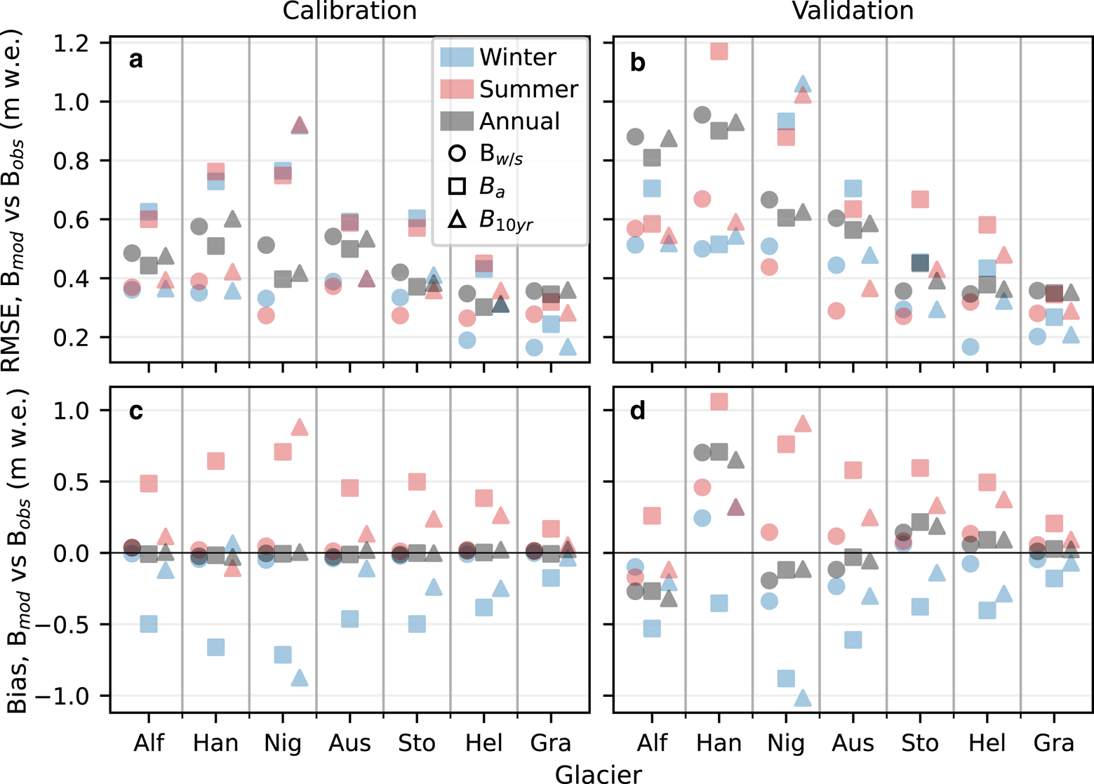
Figure 5. Model performance for each glacier in terms of RMSE (a, b) and mean bias (c, d) between modelled (posterior predictive median) and observed seasonal (winter in blue, summer in red) and annual (in grey) surface mass balance over calibration (a, c) and validation (b, d) periods for parameter estimation experiments B w/s (circle), B a (triangle) and B 10yr (square). Glaciers are sorted from west to east along a maritime to continental climate gradient.
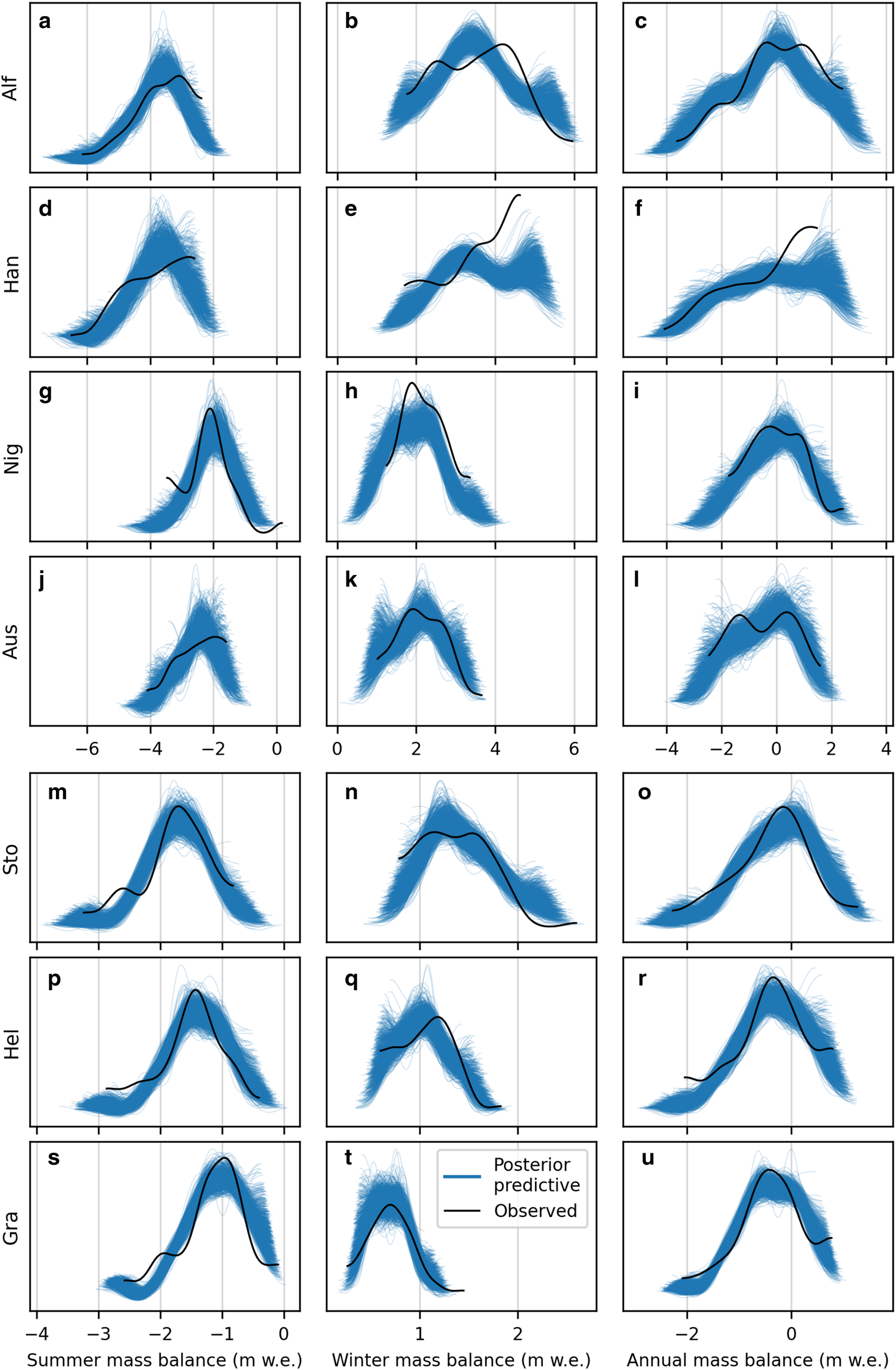
Figure 6. Probability density functions for mass balances in the B w/s experiment for 1000 posterior predictive samples (blue lines) and observations (black lines). Summer, winter and annual mass balance (m w.e.) are shown from left to right for each glacier. Glaciers are sorted from west to east along a maritime to continental climate gradient.
When considering the ensemble of glaciers, the three experiments display similar performance in modelling annual SMB over the calibration and validation years in terms of RMSE and bias between modelled and observed SMB (Fig. 5). Posterior distributions for B w/s give the lowest RMSE and bias for seasonal SMB. Overall, B a and B 10yr show a bias in the magnitudes of modelled seasonal balances, with higher (less negative) summer balances and lower (less positive) winter balances than observed. The underestimation of the magnitudes of seasonal SMB for B a and B 10yr is in line with parameter values of posterior distributions that promote lower ablation and accumulation compared to B w/s. B a shows a larger bias in seasonal SMB compared to B 10yr, and higher RMSE for most glaciers. B a appears to systematically favour mass-balance scenarios characterised by low ablation and low accumulation, in line with the lower parameter values of the posteriors in this experiment (Fig. 4).
RMSE is typically lower for the calibration period than the validation period (Fig. 5), which is not unexpected given that posteriors are informed by observations in the calibration period. Overall, the lowest RMSE is found for the three most continental glaciers (Storbreen, Hellstugubreen and Gråsubreen), and the largest deterioration in RMSE from the calibration to the validation period is found for the most maritime glaciers (Ålfotbreen and Hansebreen). For Ålfotbreen, observed seasonal and annual SMB is generally within the range of predicted values for the calibration years, while the correspondence is poor for some years of the validation period (e.g. too low winter balance in 1960s and 70 s, too negative summer balance in the 1970s and too high winter balance in the 2010s; Fig. A4).
The PDFs of posterior predictive samples of modelled mass balances (Figs. 6, A1 and A2) describe the probability distribution of mass balances over the observational period. For a well-performing and robust model, the bulk of PDFs of the posterior predictive samples should reflect the PDF of the observations. For B w/s, posterior predictive PDFs encompass the PDF of observations to a degree for most glaciers and observations, although discrepancies are visible in all cases (Fig. 6). For some ranges of mass balance, PDFs of posterior predictive samples do not encompass the PDF of observations. This implies that the model under- or overestimates SMB such that the observed SMB is not within the distribution of modelled SMB (e.g. as for Ålfotbreen for many years in the 1960s and 70s; Fig. A4). For instance, winter balance of Nigardsbreen shows predicted values around 0.5–1 and 3.5–4 m w.e., while the PDF of observations is constrained between 1–3.5 m w.e. and shows a higher density than posterior predictive PDFs in this range (Fig. 6h). For Hansebreen, correspondence between posterior predictive and observed PDFs is particularly poor, e.g. posterior predictive samples show a high frequency of large winter balances (>5 m w.e.), while the frequency of winter balances in the range 3.5–4.5 m w.e. is lower than observed (Fig. 6e). The consequence is that annual SMB (Fig. 6f) is underrepresented in the range 0-1.5 m w.e. and overrepresented in the range 1.5–3 m w.e., which indicates that annual SMB for Hansebreen is overestimated in several years. Generally, B w/s shows better correspondence for Austdalsbreen and the continental glaciers (Figs. 6j-l) than for Ålfotbreen, Hansebreen and Nigardsbreen (Figs. 6a–i).
B a (Fig. A1) yields similar results as B w/s in terms of modelled annual SMB, but with slightly higher spread such that PDFs of observed annual SMB are to a larger degree encompassed by posterior predictive samples (e.g. Ålfotbreen and Hansebreen). However, PDFs of posterior predictive samples for winter and summer balances are shifted towards low magnitudes and do not show correspondence with observations. This is in line with the low mass-turnover parameter values for B a and systematic bias in modelled seasonal balances (Fig. 5). PDFs of posterior predictive samples of B 10yr (Fig. A2) show an extremely large spread in comparison to B w/s and B a and quite high densities towards low values of seasonal balances.
We assess the performance improvement achieved through posterior inference in the three experiments by evaluating the difference between RMSE of the posterior predictive median (predictions using joint posterior distributions) and RMSE of the prior predictive median (predictions using joint prior distributions; Fig. 7). A positive performance improvement indicates that the posterior distribution improves modelled SMB compared to using the prior distribution and reflects the added benefit of using the observational data in parameter estimation as opposed to no data at all. Over the calibration period, all experiments show a performance improvement (reduction in RMSE) in terms of modelling annual SMB across all glaciers (Figs. 7a–c). The same is true for the validation period (Figs. 7d–f), except for Hansebreen. B w/s is the only experiment where posterior inference consistently improves modelling of seasonal SMB over the calibration period, and largely also over the validation period. Although both B a and B 10yr give an overall performance improvement in modelling annual SMB, in many instances, the performance in modelling underlying seasonal balances has worsened compared to using the prior distribution.

Figure 7. Performance improvement in terms of percentage reduction in RMSE of posterior predictive median compared to RMSE of prior predictive median for each glacier and experiments B w/s (a, d), B a (b, e) and B 10yr (c, f) in calibration (a–c) and validation (d–f) periods. Positive performance improvement (reduction in RMSE, up to 100%) reflects improvement in model performance when using posterior compared to prior distributions to model mass balances. Negative performance improvement (increase in RMSE, up to −∞%) reflects deterioration in model performance.
5.3. Modelled surface mass balance, 1960–2020
The modelled SMB indicates a net mass loss for all glaciers over the period 1960–2020 (Figs. 8 and 9). Nigardsbreen is the only glacier that is in near balance. Modelled (in terms of posterior predictive median) average annual SMB is similar across experiments (Fig. 8). B a and B 10yr generally give lower magnitudes of summer and winter balances than B w/s, with B a showing the lowest magnitudes overall. All experiments illustrate a large difference in mass turnover from the maritime to continental glaciers.

Figure 8. Average rates of modelled (posterior predictive median) winter, summer and annual mass balance over the period 1960–2020 for each glacier and parameter estimation experiment B w/s, B a and B 10yr. Glaciers are sorted from west to east along a maritime to continental climate gradient.

Figure 9. Cumulative annual mass balance for each glacier and experiments B w/s, B a and B 10yr over their respective period of glaciological mass-balance observations. Shaded areas represent credible intervals in terms of the 90% highest posterior density interval. Black lines indicate medians. Zero is set to the first year of the calibration period (1990). Grey vertical lines indicate the start (1990) and end (2009) of the calibration period.
The three experiments give similar results in terms of modelled cumulative SMB, but with different margins of uncertainty (Fig. 9). Uncertainty in modelled SMB (credible region in Fig. 9, which is given in terms of the 90% highest posterior density interval; the shortest interval that spans 90% of the density of the distribution) from propagation of parameter uncertainty for B w/s and B a is comparable. Considering the glaciers with observation records beginning in the 1960s, uncertainty in modelled SMB for B w/s and B a is generally higher for Ålfotbreen and Nigardsbreen, compared to Storbreen, Hellstugubreen and Gråsubreen. Across glaciers, B 10yr gives the highest uncertainty in modelled SMB. The largest difference between experiments is found for the small continental glacier Gråsubreen, where the 90% credible interval of cumulative annual SMB is an order of magnitude larger for B 10yr compared to B w/s and B a.
Modelled and observed annual SMB correspond well over the period 1960s–2020 for Storbreen, Hellstugubreen and Gråsubreen, and over the shorter records (1980s–2020) of Hansebreen and Austdalsbreen (Fig. 10). The agreement between modelled and observed annual SMB is more variable over time for Ålfotbreen and Nigardsbreen, e.g. annual SMB is generally underestimated (more negative) for Ålfotbreen from the early 1960s to the late 1970s but shows better correspondence in the subsequent decades (Figs. 9a, 10a and A4). B a shows a more or less consistent underestimation of the magnitude of summer balance over the period of available observations (Fig. 10), in line with the systematic bias found for modelled seasonal balances (Figs. 5c and d). A similar underestimation is visible for B 10yr for some glaciers (Nigardsbreen, Storbreen, Hellstugubreen and the shorter record of Austdalsbreen). For Storbreen, Hellstugubreen and Austdalsbreen, the magnitudes of seasonal balances for B 10yr are in general higher than for B a (Fig. 8), such that the underestimation is less severe. However, for Nigardsbreen, B 10yr displays a greater underestimation of modelled ablation than B a, which is also reflected in the bias between modelled and observed seasonal balances over the calibration and validation periods (Figs. 5c and d). For both B a and B 10yr, underestimation of the magnitude of summer balance is counteracted by an underestimation of the magnitude of winter balance, such that the resulting modelled annual SMB is comparable across experiments (Figs. 8 and 5c and d).

Figure 10. Cumulative difference between median of modelled (posterior predictive) and observed summer (red) and annual (black) mass balance for each glacier for experiments B w/s (solid lines), B a (dashed lines) and B 10yr (dotted lines).
6. Discussion
6.1. Prior and likelihood influence on posterior
Observations influence the posterior distribution through the likelihood function. We highlight three aspects that distinguish the datasets used in each experiment and that influence the effect of the likelihood (observations) on the posterior distribution: (1) the number of observations, (2) the mass-balance information and (3) the observational uncertainty. For B w/s and B a, posterior distributions are strongly constrained compared to B 10yr, which indicates that posteriors are more influenced by the likelihood (observations) than in the B 10yr experiment. B w/s and B a show lower posterior uncertainty compared to B 10yr due to the combination of the three factors: (1) a larger number of observations which increases the relative importance of the likelihood in posterior inference (Gelman and others, Reference Gelman2014), (2) lower equifinality in the mass-balance information and (3) lower observational uncertainty. In all experiments, accounting for observational uncertainty aggravates equifinality because we are searching for parameter values that explain a wider range of probable observations. Posterior distributions for B 10yr show high uncertainty, not only as a result of the limited number of observations but also due to the combination of significant equifinality in the mass-balance information and high observational uncertainty.
Due to the combination of the three mentioned factors, B 10yr posteriors show a wide range of probable parameter values (Fig. 4). Although posterior distributions for B w/s and B a are more constrained than B 10yr, equifinality is still reflected in the correlation between parameter values (Figs. A5 and A6) and in the difference in the spread of distributions between parameters. Overall, posteriors of P corr are more constrained than posteriors of T corr and MF snow. P corr alone largely controls accumulation of snow over the glaciers since winter temperatures are mostly below the snow/rain threshold (Fig. 2). Ablation, however, is controlled by both T corr and MF snow, such that there is a strong correlation between these two parameters (Figs. A5 and A6) and thus higher uncertainty in posteriors. For B w/s, distributions of P corr are especially narrow because the posterior is informed by observations of winter balance which are assigned lower uncertainties than summer balance observations.
Since posteriors of B w/s and B a seem to be highly constrained by the likelihood (observations) in our formulation of the Bayesian model, we would expect that our choice of prior has little influence in posterior inference in these experiments. We investigate posterior sensitivity to the choice of prior distribution for three glaciers across the maritime-continental climate gradient (Ålfotbreen, Nigardsbreen and Gråsubreen) by performing inference with low and high priors for parameters P corr and MF snow in each experiment. The sensitivity experiment illustrates the influence on the posterior for a low or high mass-turnover prior. The low and high priors were constructed from the original priors, but with means shifted up or down by one standard deviation of the original priors, e.g. such that the high (low) prior for MF snow was a truncated normal distribution with a mean of 5.6 (2.6) mm w.e.$^\circ$ C−1d−1.
For B w/s and B a, posteriors display similar properties regardless of the choice of prior (e.g. for Nigardsbreen in Fig. 11) which implies that the posterior distribution is highly influenced by the likelihood (observations). Our choice of weakly informative priors and the assigned low observational uncertainties for B w/s and B a produce posterior distributions that approach standard maximum likelihood estimates and thus reflect a narrow range of values that minimise the difference between observed and modelled SMB (Eqn (13)). For B a, the model seemingly achieves a better fit between observed and modelled annual SMB with smaller magnitudes of accumulation and ablation. This may be due to limitations in the model, e.g. simplified process representation, lack of resolution and changes in hypsometry and incremental updates of glacier areas. Since posteriors for B a are largely driven by the likelihood, we could expect that the bias of B a towards low mass-turnover parameter values would be similar in standard maximum likelihood estimation.

Figure 11. Marginal posterior probability distributions for P corr (a), MF snow (b) and T corr (c) for Nigardsbreen for experiments B w/s, B a and B 10yr using different priors (high, original and low). Prior distributions for each parameter are shown in grey. Markers indicate medians of posterior distributions, while bold and thin lines indicate interquartile range and credible interval (in terms of the 95% highest posterior density interval), respectively.
In contrast to B w/s and B a, prior influence on the posterior for B 10yr is pronounced, with marginal posteriors displaying a shift towards low or high values depending on the choice of prior. B 10yr could essentially have the same effect of favouring low mass-turnover parameter values as B a. This indication is supported by the results for Nigardsbreen, where posteriors for B 10yr and B a adopt values in the low range of the prior, in contrast to the posterior for B w/s. The low accumulation, low ablation parameter values for Nigardsbreen achieve a significantly lower RMSE for annual SMB than in the B w/s experiment (Figs. 5a and b), but give a large bias in seasonal balances (Figs. 5c and d, 10c and A1). However, the tendency to favor low mass-turnover scenarios is generally less pronounced for B 10yr due to the comparatively stronger prior influence and weaker influence of the likelihood (observations). The high parameter uncertainty and sensitivity to choice of prior distribution in the B 10yr experiment implies that the number of unknown parameters is at the upper limit of what can be reliably estimated using decadal resolution satellite-borne geodetic observations with their characteristic uncertainty. Increasing the number of unknown parameters could aggravate equifinality such that the inferred posterior distributions would largely reflect the priors.
6.2. Parameter values
We compare parameter values for B w/s across glaciers as this experiment most correctly represents accumulation and ablation. For all glaciers, values of P corr for B w/s (medians range from 1.06 to 1.55, see Tables S1–S3) indicate that seNorge_2018 may underestimate winter precipitation. To our knowledge, no formal evaluation of seNorge_2018 in glacio-hydrological modelling in remote data-void regions has been performed. However, considering previous evaluation of winter precipitation in seNorge1 (Engelhardt and others, Reference Engelhardt, Schuler and Andreassen2012), our results are in line with lower precipitations sums in seNorge_2018 compared to seNorge1 (Fig. 2). P corr shows a trend from higher to lower values from coastal (Ålfotbreen and Hansebreen) to more inland glaciers (Nigardsbreen and Austdalsbreen) across experiments. This indicates that seNorge_2018 may not adequately capture the strong longitudinal precipitation gradient in southern Norway. A similar pattern in values of P corr from west to east over the continental glaciers also suggests that orographic effects over the central mountain ranges may not be accurately represented. Although parameter values suggest underestimation of precipitation in seNorge_2018, strong conclusions regarding the magnitude of underestimation should not be drawn based on these values. Parameter values are influenced by the model limitations discussed earlier, as well as potential biases in observations and choice of calibration period. Other processes that may influence accumulation, such as redistribution of snow by wind or avalanching, are also not included in the model.
Values of T corr for B w/s indicate a slight overestimation of temperature in seNorge_2018 for maritime glaciers and an underestimation for the westernmost continental glaciers. However, in addition to the limitations in model structure and potential influences on parameter values mentioned earlier, general statements about the quality of seNorge_2018 temperature are even more precarious due to compensating effects between T corr and MF snow on modelled ablation. Considering MF snow, maritime glaciers generally exhibit higher values than continental glaciers, in agreement with the findings of Zhang and others (Reference Zhang, Liu and Ding2006) for degree-day factors of maritime and continental glaciers in western China. Engelhardt and others (Reference Engelhardt, Schuler and Andreassen2014) found a similar pattern in parameters controlling melt across Åfotbreen, Nigardsbreen and Storbreen, but parameter values are not directly comparable to this study due to differences in the model structure. For Storbreen and Hellstugubreen, which have lowest values of MF snow, we would expect higher values of MF snow without the compensating effect of T corr.
6.3. Effect of observations on modelled mass balance
The magnitudes of seasonal balances are generally underestimated (too low) for B a (Figs. 5, 10 and A1), due to parameter values promoting lower accumulation and ablation (Fig. 4). Underestimation of the magnitude of ablation implies that also summer meltwater runoff would be underestimated for B a. B 10yr also shows underestimation of magnitudes of summer and winter balances, which is in line with findings of Rounce and others (Reference Rounce, Hock and Shean2020a) for glaciers in High Mountain Asia with parameters calibrated with 20-year geodetic mass-balance observations. B w/s is the only experiment that adequately resolves seasonal balances (Figs. 5 and 6) and consistently improves modelled seasonal balances (Fig. 7) because posteriors are informed by winter and summer balance observations. The overall better performance in terms of median values of B 10yr in modelling seasonal SMB compared to B a (Figs. 5 and 10) could be attributed to a choice of priors that produce posteriors centered around the same values as B w/s, and thus give decent estimates of accumulation and ablation.
B a and B 10yr (which is essentially an aggregation of annual SMB observations) give decent mass-balance estimates (Figs. 5, A1 and A2) and improvement of annual SMB (Fig. 7) since posteriors are informed by annual SMB observations. However, this does not necessarily improve performance in modelling seasonal balances since parameter values that give the best estimates of annual SMB do not necessarily reproduce seasonal variations. Nevertheless, due to the equifinality in the mass-balance model, B a and B 10yr give estimates of annual SMB that are in line with those achieved by resolving seasonal balances in the B w/s experiment.
Overall, all experiments improve estimates of annual SMB compared to employing parameter values based on prior knowledge (Fig. 7). A performance improvement does not necessarily imply a good model performance, but rather reflects the added value of using the observations in calibration for a given prior. Across experiments and glaciers, deterioration in RMSE reflects that a posterior centred around the median of the prior distribution would give lower RMSE than the inferred posterior. The deterioration in RMSE in seasonal and annual SMB over the validation period for some glaciers (e.g. Hansebreen; Figs. 7d–f) reflects that posterior parameter values are less representative over this period than the prior values. B 10yr posteriors are clearly sensitive to the choice of prior (Fig. 11) but improve modelling of annual SMB for most glaciers and priors we evaluated (Fig. 12). Although B 10yr represents a mass-balance signal of low temporal resolution and high uncertainty, posterior distributions informed by such observations yield improved estimation of annual SMB compared to employing parameter values based on prior knowledge alone. In the low and original prior cases for Ålfotbreen and Gråsubreen, B 10yr also improves modelled seasonal SMB because posterior parameter values also produce better representations of accumulation and ablation.

Figure 12. Performance improvement for B 10yr in terms of percentage reduction in RMSE of posterior predictive mean compared to RMSE of prior predictive mean for calibration (a) and validation (b) periods for Ålfotbreen (Alf), Nigardsbreen (Nig) and Gråsubreen (Gra) using high, original and low priors. Positive performance improvement (reduction in RMSE, up to 100%) reflects improvement in model performance when using posterior compared to prior distributions to model mass balances. Negative performance improvement (increase in RMSE, up to −∞%) reflects deterioration in model performance.
Although B 10yr gives decent estimates of annual SMB in terms of median values, the modelled uncertainty is significantly higher than for B w/s and B a (Fig. 9). The high parameter uncertainty in the B 10yr experiment leads to a considerably higher uncertainty (standard deviation) in mass-balance sensitivity compared to the other experiments (by a factor of 1.2–3.1 compared to B w/s, see Supplementary Material for details). This uncertainty reflects the parameter uncertainty, which is again determined by the influence of the likelihood (given our prior formulations). High temporal resolution, low uncertainty observations (B w/s and B a) correspond to low uncertainties in modelled SMB, while low temporal resolution, high uncertainty observations (B 10yr) yield high modelled uncertainties. For B w/s and B a, uncertainty in modelled SMB is higher for Ålfotbreen and Nigardsbreen compared to continental glaciers. This reflects that glaciological observations of high mass-turnover glaciers are generally associated with higher uncertainty (Table 2). For B 10yr, the difference in uncertainty in modelled SMB between glaciers generally corresponds to the difference in magnitudes of observation uncertainties (Table 2 and Fig. 9). Gråsubreen, which shows the largest difference in modelled uncertainties between B w/s/B a and B 10yr, has particularly low uncertainty in glaciological observations and large uncertainty in geodetic observations. For satellite-borne geodetic observations, uncertainty is in general higher for smaller (e.g. Gråsubreen) compared to larger (e.g. Nigardsbreen) glaciers due to the combination of limited spatial coverage of elevation change estimates, high uncertainty in the temporal evolution of the glacier area, and uncertainty in the volume-to-mass density conversion (Hugonnet and others, Reference Hugonnet2021).
Modelled mass balances for Hansebreen and Austdalsbreen are validated on fewer observations than for the other glaciers. The difference in bias over the validation period between the similar (in terms of hypsometry and area) neighboring glaciers Ålfotbreen and Hansebreen (Fig. 5d) could be partly explained by their validation periods. For these two glaciers, the late 1980s to mid-1990s was a period of predominant mass gain, followed by two decades of predominantly large mass losses from 2001 (Fig. 3). While the validation period for Ålfotbreen covers years of moderate positive and negative balances from 1963 to 1990, Hansebreen is mainly validated on a shorter period of more extreme mass-balance years (end of 1980s and 2010s). This could also explain the particularly poor correspondence between modelled and observed mass-balance distributions for Hansebreen (Figs. 6d–f) and deterioration of RMSE in the validation period (Fig. 7).
6.4. Parameter and model robustness
An interesting result of posterior inference with our model is that posterior distributions of B a and B w/s are not equifinal solutions of each other. We would expect high probability regions of posteriors of B w/s and B a to show overlap as both posteriors produce decent estimates of annual SMB (e.g. Figs. 5 and 10). We believe that the discrepancy is due to a combination of two factors: (1) limitations in the model structure (e.g. lack of complexity, processes representation and limited spatial resolution) and the number of parameters estimated, such that simultaneous reproduction of the most accurate representation of annual and inter-annual variations is not possible; and (2) that the assigned uncertainties in B w/s and B a are too low, such that the influence of the likelihood in our Bayesian model is too strong.
We only estimate three parameters due to the low temporal resolution and high uncertainty in B 10yr, which limits the variability in SMB that can be achieved with our simple model. Although we find decent results in terms of median values, PDFs of B w/s and B a suggest that observed values are in many cases outside the spread of predictions, which indicates that these models are not particularly robust. This suggests that the spread in the error term (Eqn (9)) to which we assign the observation uncertainty may be too low to produce robust predictions for B w/s and B a given our mass-balance model. Options to increase robustness of B w/s and B a could be to explore the use of larger variance than the reported observation uncertaintyor whether other distributions than the normal distribution are more appropriate for the likelihood or prior. We investigated the use of Student's t distributions, which are more heavy tailed than the normal distribution, for the likelihood in the B w/s and B a experiments for some glaciers (see Supplementary Material for details). We found that using Student's t distributions for the likelihood gives posterior distributions centred around the same values, but with larger spread, thus giving a broader range of posterior predictive samples. However, we still found the same bias in B a towards low mass-turnover parameter values in the tests we performed.
B w/s yields a decent estimation of seasonal and annual SMB, but the overall reduction in performance from calibration to validation period (Fig. 5) reflects a lack of robustness of parameter values over time. The deterioration in performance is especially visible for maritime glaciers that have high mass-balance gradients (e.g. for Ålfotbreen; Fig. A4). This highlights a general issue of temperature index models concerning the representativeness of constant parameter values, e.g. those of melt factors, over longer time scales where meteorological conditions may vary. Melt factors implicitly account for the relative contribution of the various energy-balance components and therefore vary in both space (e.g. aspect, elevation) and time (e.g. change in albedo with snow/ice surface properties; Hock, Reference Hock2003, Reference Hock2005). Calibrated melt factors may be representative of climatic conditions specific for the calibration period, but not necessarily beyond (Gabbi and others, Reference Gabbi, Carenzo, Pellicciotti, Bauder and Funk2014). Although we attempt to reduce bias in parameter values to specific climatic conditions by employing a calibration period that encompasses years of mass-balance variability, results nevertheless indicate a lack of representativeness of parameter values in certain time periods. The underestimation of SMB in the 1960s and 1970 s is not only prominent for Ålfotbreen, but also visible for the other glaciers with records dating back to the 1960s (Figs. 9 and 10). This bias could also be due to unresolved geometry changes in the model (constant hypsometry and incremental area updates), but we would not expect this to be the main influence as all glaciers have outlines from the 1960s (Table 1) and surface elevation changes over the glaciers are limited (−2.2 m to −15.8 m for Nigardsbreen and Hellstugubreen, respectively, from the 1960s to the 2010s Andreassen and others (Reference Andreassen, Elvehøy, Kjøllmoen and Belart2020)). Alternatively, there could be biases in the climate dataset specific to certain time periods, e.g. due to varying quality of meteorological observations used in the reanalysis, that are not captured by the constant temperature and precipitation corrections. Still, we argue that capturing parameter uncertainty from uncertainty in observations is an indirect way to, at least partly, reflect the variability of parameter values over time. Employing more robust formulations of the Bayesian model could make the model predictions more robust to these variations, at a cost of increased uncertainty in modelled mass balances.
Our results show that parameter estimation employing annual observations with low uncertainty or decadal observations with high uncertainty could produce decent estimates of annual SMB, and we would thus expect such observations to be useful in constraining net glacier mass changes, e.g. in determining future sea-level rise. However, the underlying seasonal mass changes may not be resolved using these observations. To improve estimates of accumulation and ablation, annual and decadal mass-balance observations could be used in combination with observations that constrain accumulation and/or ablation, e.g by using independent data on snow distribution (e.g. Geck and others, Reference Geck, Hock, Loso, Ostman and Dial2021). However, such observations are generally lacking, particularly at the scale of individual glaciers. High-quality, high-resolution climate data in complex terrain, or widespread, higher resolution mass-balance observations are needed to properly resolve interannual and interseasonal variations in mass balance.
7. Conclusions
We modelled SMB of seven glaciers in southern Norway over the period 1960–2020 using a temperature index model. The glaciers are located along a maritime-to-continental climate gradient and have long-term glaciological SMB records. To explore how the use of distinct mass-balance observations affects model calibration, we applied a Bayesian framework to estimate three sets of parameters for each glacier based on three representations of the respective glaciological records: seasonal, annual and 10-year average SMB. For seasonal and annual mass balances, we employed associated uncertainties from the glaciological records. Ten-year average SMB represented our analogue to geodetic mass balance based on satellite remote sensing and was thus assigned uncertainties characteristic to such observations.
Posterior parameter distributions are strongly dependent on the observations used in parameter estimation and, in the experiment using 10-year average SMB, also on the choice of prior distribution. The marginal posterior distributions of the precipitation correction factor indicates that the seNorge_2018 climate dataset may underestimate winter precipitation over the westernmost glaciers.
All datasets demonstrated decent performance in modelling annual SMB and generally improved estimates of annual SMB compared to using parameter values based on prior knowledge. However, using 10-year average SMB displayed higher uncertainty in modelled mass balance and in mass-balance sensitivity to changes in climate forcing due to considerable parameter uncertainty.
Reliable estimates of the magnitude of accumulation and ablation were only achieved using seasonal balances to constrain parameters. However, model performance varied over time due to the application of constant parameter values and limited robustness of the Bayesian model. Using annual mass-balance observations consistently favoured parameter values that promote low accumulation and ablation. Consequently, magnitudes of summer and winter balances were on average around 20% lower over the period 1960–2020 using annual compared to seasonal balances in parameter estimation.
Similar to the use of annual SMB, the use of 10-year average SMB also tended to underestimate magnitudes of accumulation and ablation but was restricted by the influence of the prior distribution. Nevertheless, our results demonstrate that high-uncertainty geodetic observations, which typically represent decadal snapshots of glacier mass change, can be used in parameter calibration to improve model results of annual mass balance. Since our representation of decadal mass-balance observations are constructed from glaciological records, the actual performance of satellite-borne geodetic observations will depend on the quality of these observations.
Propagation of parameter uncertainty revealed large differences in uncertainty in modelled SMB between the observational datasets, up to an order of magnitude for the small, continental glacier Gråsubreen. However, for the larger, more maritime glacier Nigardsbreen, uncertainty in modelled SMB was comparable between datasets due to higher mass-balance variability and similar observational uncertainty in glaciological and geodetic observations.
We underline that our findings are based on a limited sample of glaciers and are conditional on the specific model structure in this study. Generalisation to other model structures and glaciers should thus be made with caution. Nevertheless, our findings highlight that the purpose of modelling should be considered when choosing the type of mass-balance data to be used in model calibration. For reliable predictions of the timing and magnitude of runoff, e.g. in assessment of climate change impacts on freshwater availability, evaluating the performance of models on seasonal mass balances is important. Therefore, more extensive and robust seasonal mass-balance data are needed to both improve and evaluate model performance on seasonal scales.
Supplementary material
The supplementary material for this article can be found at https://doi.org/10.1017/jog.2023.62.
Data
The source code of the model is available in the GitHub repository https://github.com/khsjursen/BI_glacier_mb_model. seNorge_2018 is available for download at https://thredds.met.no/thredds/catalog/senorge/seNorge_2018/catalog.html. Mass balance observations can be found at http://glacier.nve.no/glacier/viewer/ci/en/ and time series of glacier outlines used in this study are available in the model GitHub repository.
Acknowledgements
This study is a contribution to the JOSTICE project funded by the Norwegian Research Council (RCN grant #302458). We thank Hallgeir Elvehøy and Bjarne Kjøllmoen at NVE for providing mass-balance observations and time series of glacier outlines of Ålfotbreen, Hansebreen, Nigardsbreen and Austdalsbreen, and Markus Engelhardt for providing MATLAB code that the implementation of the mass-balance model is partly based upon. We would also like to recognise the Western Norway University of Applied Sciences (HVL) for providing computational resources and the managers of the HVL cluster for technical support. In addition, we thank Gregoire Guillet, David Rounce and Lilian Schuster for evaluating our manuscript and providing constructive feedback that has both improved the quality and clarity of the paper.
Author contribution
KHS developed the code for the mass-balance model and Bayesian parameter estimation routine, performed the MCMC simulations and initial analysis, and prepared the figures, tables and initial draft of the article. TD, AT, TVS and LMA read and edited the article, and provided input for additional analyses. LMA provided mass-balance observations and time series of glacier outlines for Storbreen, Hellstugubreen and Gråsubreen.
Appendix A. Additional figures

Figure A1. Probability density functions for mass balances in the B a experiment for 1000 posterior predictive samples (blue lines) and observations (black lines). Summer, winter and annual mass balance (m w.e.) is shown from left to right for each glacier. Glaciers are sorted from west to east along a maritime to continental climate gradient.

Figure A2. Probability density functions for mass balances in the B a,10yr experiment for 1000 posterior predictive samples (blue lines) and observations (black lines). Summer, winter and annual mass balance (m w.e.) is shown from left to right for each glacier. Glaciers are sorted from west to east along a maritime to continental climate gradient.

Figure A3. Model performance per glacier in terms of median absolute deviation (MAD) (a, b) and median bias (c, d) between modelled (posterior predictive median) and observed seasonal (winter in blue and summer in red) and annual (grey) surface mass balance over calibration (a, c) and validation (b, d) periods for experiments B w/s (circle), B a (triangle) and B 10yr (square). Glaciers are sorted from west to east along a maritime to continental climate gradient.

Figure A4. Posterior predictive samples (100 samples) in B w/s experiment of winter (blue), summer (red) and annual (grey) mass balances for Ålfotbreen 1963–2020. Observations of winter (dotted line), summer (dashed line) and annual (solid line) mass balances are shown as black dots. Grey vertical lines indicate the start (1990) and the end (2009) of the calibration period.

Figure A5. Joint posterior distributions of pairs of parameters for Ålfotbreen for the three experiments B w/s (a–c), B a (d–f) and B 10yr (g–i). Parameters are melt factor for snow (MF snow; mm w.e.$^\circ$ C−1d−1), temperature correction factor (T corr; $^\circ$
 C) and precipitation correction factor (P corr; -). Lines and points indicate medians of distributions.

Figure A6. Joint posterior distributions of pairs of parameters for Gråsubreen for the three experiments B w/s (a–c), B a (d–f), and B 10yr (g–i). Parameters are melt factor for snow (MF snow; mm w.e.$^\circ$ C−1d−1), temperature correction factor (T corr; $^\circ$
 C) and precipitation correction factor (P corr; -). Lines and points indicate medians of distributions.


 Open access