


1. Introduction
A heuristic study by Mercer (Reference Mercer1968) suggesting that the West Antarctic Ice Sheet (WAIS) collapsed at least once in its history raised the question whether WAIS is currently experiencing another collapse (e.g., Hughes, Reference Hughes1975; Joughin and others, Reference Joughin, Smith and Medley2014) or whether it could collapse in the (near) future under a warming climate (e.g., Mercer, Reference Mercer1978; DeConto and Pollard, Reference DeConto and Pollard2016). Resting on a bed below sea level, the fate of the WAIS is determined by the evolution of the grounding line, ‘the junction between ice sheet and ice shelf’ (Weertman, Reference Weertman1974). Since the first analytical analysis of marine ice sheets by Weertman (Reference Weertman1974), grounding-line retreat either observed on the present-day Antarctic and Greenland ice sheets (e.g., Shepherd and others, Reference Shepherd2018; Khan and others, Reference Khan2020) or simulated with ice-sheet models (e.g., Cornford and others, Reference Cornford2015; Seroussi and others, Reference Seroussi2020), has frequently been interpreted as an indication of ice-sheet ‘instability’.
Realistic ice sheets are subject to the atmospheric and oceanic forcing that constantly varies in time on a wide range of temporal scales. As a result, the ice sheets do not attain steady states, stable or not. To add to the confusion, the terms ‘stable’ and ‘unstable’ are frequently used to describe the migration of grounding lines, i.e. they are used to describe unsteady, time-variable behavior (e.g., Shepherd and others, Reference Shepherd, Fricker and Farrell2018a). This mischaracterization might stem from the results of Weertman's(Reference Weertman1974) original analysis, which related the existence of a steady-state ice-sheet configuration and its stability to the bed slope at the location of the grounding line. He concluded that ‘[a] stable ice sheet can occur if the bed slopes away from the center of the ice sheet.’ (Weertman, Reference Weertman1974). Because the beds in many locations under the WAIS, parts of the East Antarctic Ice Sheet, and parts of the Greenland Ice Sheet slope towards the interior of these ice sheets, the grounding line positions are described as ‘unstable’ as a corollary of Weertman's result, regardless of the temporal variability of either the ice sheets or their environmental conditions.
Existing theoretical analyzes of grounding line behavior are focused on steady states of idealized configurations (e.g., Schoof, Reference Schoof2007a; Wilchinsky, Reference Wilchinsky2009; Tsai and others, Reference Tsai, Stewart and Thompson2015; Pegler and Worster, Reference Pegler and Worster2013; Pegler, Reference Pegler2018; Haseloff and Sergienko, Reference Haseloff and Sergienko2018) and questions of their stability (e.g. Schoof, Reference Schoof2012; Sergienko and Wingham, Reference Sergienko and Wingham2019; Haseloff and Sergienko, Reference Haseloff and Sergienko2022; Sergienko and Wingham, Reference Sergienko and Wingham2022; Sergienko, Reference Sergienko2022b). These studies assume specific functional forms of basal and lateral shear parameterizations, most often a power-law sliding law (e.g., Schoof, Reference Schoof2007a, Reference Schoof2007b; Schoof, Reference Schoof2012; Sergienko and Wingham, Reference Sergienko and Wingham2019, Reference Sergienko and Wingham2022) and, in the case of laterally confined (‘buttressed’) marine ice sheets, a power-law lateral shear stress (e.g., Schoof and others, Reference Schoof, Devis and Popa2017; Pegler, Reference Pegler2018; Haseloff and Sergienko, Reference Haseloff and Sergienko2018, Reference Haseloff and Sergienko2022; Sergienko, Reference Sergienko2022a). Consequently, results of these studies apply only to the steady-state behavior of these particular forms of basal and lateral shear stress formulations.
To date, investigations of the temporal evolution of ice sheets, especially under changing climatic forcing and for realistic regional or continental configurations, require the use of numerical simulations (e.g., Cornford and others, Reference Cornford2015; Seroussi and others, Reference Seroussi2017, Reference Seroussi2020). The results of these numerical studies are complex and are typically interpreted in terms of the conceptual results of the theoretical analyzes, even though those are applicable to steady-state conditions only. In particular, rapid grounding line retreat is often identified as a manifestation of the instability of grounding lines on retrograde beds. Key conclusions drawn from numerical studies include: (i) rapid grounding-line retreat is triggered by loss of buttressing ice shelves (e.g., Favier and others, Reference Favier, Pattyn, Berger and Drews2016; Gudmundsson and others, Reference Gudmundsson, Paolo, Adusumilli and Fricker2019), (ii) the rate of grounding-line migration strongly depends on the choice of the sliding law (e.g., Brondex and others, Reference Brondex, Gagliardini, Gillet-Chaulet and Durand2017; Sun and others, Reference Sun2020; Åkesson and others, Reference Åkesson, Morlighem, O'Regan and Jakobsson2021), (iii) stochastic variability to climate forcing can trigger rapid grounding line retreat (e.g., Christian and others, Reference Christian, Robel and Catania2022).
Reconciliation of these modeling results with our conceptual understanding of grounding line dynamics requires an extension of the existing analytical framework to the time-evolving behavior of marine ice sheets with variable basal and lateral shear stress parameterizations. To develop this framework, we derive expressions for the ice flux at the grounding line, the rate of the grounding-line migration, and stability conditions for steady-state configurations. As an illustration, we apply it to compare a laterally confined marine ice sheet subject to two different sliding laws: i) a composite viscous and Coulomb-style sliding law proposed by Zoet and Iverson (Reference Zoet and Iverson2020) on the basis of the results of laboratory experiments (hereafter referred to as Zoet-Iverson sliding law) and ii) a power-law sliding law (Weertman, Reference Weertman1957; Fowler, Reference Fowler1981). The lateral shear is described by a power law (e.g., Raymond, Reference Raymond1996).
In this framework, all terms of the steady-state expressions can be written in closed form. For given bed topography, basal and lateral shear stresses and environmental characteristics (i.e. surface accumulation and submarine melting), steady-state configurations can be determined (if they exist) and their stability can be established. Capturing the temporal evolution of ice sheets analytically is not possible because there is no closed form expression for a time-variant buttressing parameter (Haseloff and Sergienko, Reference Haseloff and Sergienko2018). Thus, investigations of the response of buttressed marine ice sheets to temporal variations in forcing need to rely on numerical simulations to produce quantitative results, but the expressions derived here provide insights into the controls on grounding line behavior and can guide our conceptual understanding.
In this study we choose to focus on the effects of stochastic variability in submarine melting. The Earth's climate has a wide range of modes of internal variability on a variety of temporal scales. For instance, the recent retreat of the grounding line of Pine Island Glacier has been attributed to decadal oceanic variability (Jenkins and others, Reference Jenkins2018); retreats and advances of the grounding lines in the Pacific sector of West Antarctica exhibit strong variability on this timescale as well (Christie and others, Reference Christie, Steig, Gourmelen, Tett and Bingham2023). Global circulation models indicate that conditions in the Southern Ocean exhibit variability on centennial timescales (e.g., Latif and others, Reference Latif, Martin and Park2013). Numerical studies investigating the response of grounding lines to variability in climate forcing using realistic (e.g., Hoffman and others, Reference Hoffman, Asay-Davis, Price, Fyke and Perego2019; Robel and others, Reference Robel, Seroussi and Roe2019) and idealized configurations (e.g., Christian and others, Reference Christian, Robel and Catania2022; Felikson and others, Reference Felikson, Nowicki, Nias, Morlighem and Seroussi2022) indicate a substantially different grounding-line behavior compared to that without any variability in the climate forcing.
Our results show that a classification of the grounding-line behavior into ‘stable’ or ‘unstable’ loses its meaning when considering its time-dependent behavior. We find that starting from a stable steady-state configuration, the grounding line of a buttressed marine ice sheet can exhibit irregular oscillations as well as an unstoppable retreat depending on the specifics of the stochastic variability. The results of our linear stability analysis indicate that stability conditions of steady-state marine ice sheets depend on a large number of parameters combined in a complex way, and in contrast to the results of Weertman (Reference Weertman1974) and Schoof (Reference Schoof2012), stability or instability of a steady state cannot be easily inferred from a simple external characteristic, such as the bed slope at the grounding line. Consequently, terms ‘stable’ and ‘unstable’ are not useful for description of the grounding line behavior of realistic ice sheets.
The manuscript is organized as follows: After a model description in section 2, we introduce the analytical framework for derivations of the expressions of the ice flux at the grounding line, the rate of the grounding line migration and the steady-state stability conditions for arbitrary forms of the basal and lateral shears (section 3). In section 4 we apply the developed framework to a marine ice sheet with Zoet-Iverson sliding law and compare its steady-states with a marine ice sheet with Weertman sliding law. These configurations are exposed to stochastic variability in submarine melting in section 5. Readers less interested in the mathematical aspects of the analysis can proceed to sections 6–7 where we summarize the results and provide their physical interpretation.
2. Model description
Following many previous studies (e.g., Schoof and others, Reference Schoof, Devis and Popa2017; Pegler, Reference Pegler2018; Haseloff and Sergienko, Reference Haseloff and Sergienko2018, Reference Haseloff and Sergienko2022), we consider a laterally confined ice stream flowing into a laterally confined ice shelf (Fig. 1).

Figure 1. Model geometry: b - bed elevation (b < 0), h - ice thickness, x d - the ice divide location, x g - the grounding line location; x c - the calving front location.
It is described by a vertically integrated and laterally averaged momentum balance under assumptions of a negligible vertical shear appropriate for ice-stream and ice-shelf flow (MacAyeal, Reference MacAyeal1989)


Subscripts indicate partial derivatives, e.g., u x = ∂u/∂x. u(x, t) is the depth- and width-averaged ice velocity; h(x, t) is ice thickness; b(x, t) is bed elevation (negative below sea level and positive above sea level); A is the ice stiffness parameter (assumed to be constant); n is the exponent of Glen's flow law, g is the acceleration due to gravity. τ b and τ w are the laterally averaged basal and the lateral shear, respectively, which can have different functional forms and dependencies on the ice stream and ice shelf. g ′ is the reduced gravity defined as

where

is the buoyancy parameter, ρ and ρ w are the densities of ice and water, respectively. x d = 0 is the location of the ice divide, x c(t) is the location of the calving front, and x g(t) is the location of the grounding line – the location where the grounded ice starts to float and form the ice shelf. The first term on the left hand side of (1a) and (1b) is the divergence of the longitudinal stress τ x = (2A −1/nh|u x|1/n−1u x)x. The basal shear τ b, and lateral shear τ w of the ice stream and ice shelf are treated as arbitrary functions, i.e.


where ξ b and ξ w represent a set of all variables that τ b and τ w may depend on – ice velocity, effective pressure (in the case of τ b) ice thickness, the ice-stream or ice-shelf width (in the case of τ w), etc. For brevity, we combine all these variables into one set and denote it ξ = {ξ b, ξ w}, with understanding that the respective function (either τ b or τ w) depends on its respective set of variables (either ξ b or ξ w).
The mass balance is


where $\dot a( x,\; \, t)$ is the net accumulation/ablation at the ice top surface and $\dot m( x,\; \, t)$
 is the net melting/refreezing rate at the ice-shelf base (we assume that melting/refreezing at the ice-stream base is negligible).
Boundary conditions at the divide x d and the calving front x c are


The conditions (6a) state that the driving stress at the divide is zero and there is no flow that enters or leaves from the left. The condition (6b) requires the longitudinal stress in the ice to balance the pressure deficit at the calving front.
At the grounding line x g the continuity conditions


(the last condition is on the longitudinal stress τ = 2A −1/nh|u x|1/n−1u x), and the flotation condition

are satisfied. The fact that the ice is grounded upstream of the grounding line and is floating downstream of it is reflected by two inequalities


Haseloff and Sergienko (Reference Haseloff and Sergienko2018) have demonstrated that the momentum balance of the ice shelf (1b) can be integrated with the boundary condition at the calving front, x c, (6b) and the continuity conditions (7). As a result, the problem can be split into two – one for the ice stream and one for the ice shelf. The boundary conditions at the grounding line are the flotation condition (8), velocity and thickness continuity conditions (7a)–(7b), and the stress continuity condition (7c) written in a form

where θ ≤ 1 is the buttressing parameter – the ratio between the backstress at the grounding line and the backstress in the absence of the ice-shelf lateral confinement, which is $\displaystyle {{1}/{2}\rho g^\prime h^2}$ . This parameter represents the effects of the laterally confined ice shelf on the stress-regime of the grounding line. It encapsulates the integrated effects of the ice-shelf dynamics, the ice-shelf mass balance, other ice-shelf parameters and calving conditions on the grounding line. Hence, θ depends on the length of the ice shelf, lateral shear τ w and its parameters ξ, the functional forms of the net accumulation/ablation and melting/refreezing rates, $\dot a$
 and $\dot m$
 , respectively, calving conditions (e.g., a prescribed calving-front position, a prescribed value of ice thickness at the calving front) and their parameters (Haseloff and Sergienko, Reference Haseloff and Sergienko2018). It also depends on the ice flux

in the ice shelf as well as at the grounding line, q(x g). In some cases (e.g., for particular forms of sub-ice-shelf melting $\dot m$ and calving conditions), it is possible to write a closed-form expressions of the buttressing parameter (Haseloff and Sergienko, Reference Haseloff and Sergienko2018, Reference Haseloff and Sergienko2022). However, there is no general expression for θ. Consequently, we treat it as an arbitrary function of a set of parameters $\varpi$
 that includes all parameters mentioned above and write $\theta ( \varpi )$
 .
.
The grounded parts of marine ice sheets can experience distinct dynamic regimes. In the first one, the divergence of the longitudinal stress (the first term on the left-hand side of (1a)) has much lower magnitude than all other terms. The driving stress (the last term on the left-hand side of (1a)) is typically large, on the order of hundreds of kPa. This dynamic regime is characteristic of very wide glaciers like Thwaites Glacier in the Amundsen Sea Embayment (West Antarctica) (e.g., Holt and others, Reference Holt2006), and laterally confined glaciers like Greenland marine outlet glaciers, Pine Island Glacier in the Amundsen Sea Embayment (e.g., Wingham and others, Reference Wingham, Wallis and Shepherd2009), ice streams flowing into the Filchner-Ronne and Amery ice shelves (e.g., King and others, Reference King, Woodward and Smith2007), and many others. Such a stress regime has been considered by Weertman (Reference Weertman1974); Wilchinsky (Reference Wilchinsky2009); Schoof (Reference Schoof2007a, Reference Schoof2007b); Schoof (Reference Schoof2012); Tsai and others (Reference Tsai, Stewart and Thompson2015); Pegler (Reference Pegler2016, Reference Pegler2018); Schoof and others (Reference Schoof, Devis and Popa2017); Haseloff and Sergienko (Reference Haseloff and Sergienko2018, Reference Haseloff and Sergienko2022); Sergienko and Wingham (Reference Sergienko and Wingham2022); Sergienko (Reference Sergienko2022b). In the second regime, the divergence of the longitudinal stress is of the same order of magnitude as the other components of the momentum balance (1a). The driving stress in this regime is typically low, on the order of several kPa. This dynamic regime is characteristic of Siple Coast ice streams flowing into the Ross Ice Shelf (West Antarctica) (e.g., Rose, Reference Rose1979; Bindschadler and Vornberger, Reference Bindschadler and Vornberger1998); it has been considered by Sergienko and Wingham (Reference Sergienko and Wingham2019). Here, we focus on the first dynamic regime and provide a brief description of the treatment of the second dynamic regime in section 3.4.
3. Framework for arbitrary forms of sliding and lateral shear
As Haseloff and Sergienko (Reference Haseloff and Sergienko2018) showed, the behavior of a buttressed marine ice sheet is described by the momentum and mass balances of the grounded part (1a) and (5a), respectively, and the boundary conditions at the ice divide (6a) and at the grounding line: the flotation condition (8) and the stress condition (10).
A scaling analysis of Schoof (Reference Schoof2007a, Reference Schoof2007b); and Sergienko and Wingham (Reference Sergienko and Wingham2022) can be directly applied here, resulting in the leading order problem of the grounded part (1a), (5)–(10)


This is an approximate model that describes the behavior of the grounded ice stream, which is buttressed by a laterally confined ice shelf. Below we derive a relationship between the ice flux at the grounding line and dynamic (stress), geometric (bed elevation and slope) and environmental conditions at the grounding line; an expression for the grounding line migration and stability conditions for steady-state configurations in terms of the general forms of the basal and lateral shears. The only condition imposed on these general forms is that they are continuously differentiable with respect to variables they depend on. We follow derivations of Haseloff and Sergienko (Reference Haseloff and Sergienko2022) and Sergienko and Wingham (Reference Sergienko and Wingham2022), and in contrast to studies based on the boundary-layer theory (Schoof, Reference Schoof2007a, Reference Schoof2012; Tsai and others, Reference Tsai, Stewart and Thompson2015) that consider configurations with shallow beds, negligible bed slopes and small accumulation rates at the grounding line, we do not make any additional assumptions apart from those under which the vertically integrated momentum balance (1) is derived.
3.1 Ice flux at the grounding line
Observing that

where q is the ice flux (11), rearranging terms in (12a), the problem (12) can be written as


where the stress-condition (12d) written in terms of q was obtained by using (13) and (14a). We assume that θ > 0. Although it is possible to write (12d) in a form permitting a negative buttressing parameter, it is unclear how realistic such a situation could be. Physically, θ < 0 implies that the ice at the grounding line is under compression and u x < 0. It is unclear which processes can determine the limit of compression, i.e. how negative u x can be. Consequently, we consider only the case of θ > 0.
For a dynamic ice sheet that evolves with time, (14d) is

As apparent from these expressions, if specific forms of the lateral shear τ w and the sliding law τ b depend on the ice velocity $\displaystyle {u = {q}/{h}}$ , the ice flux at the grounding line will be an implicit function of ice thickness h and thinning rate h t. Only if these forms are independent of the ice velocity, and the ice shelf is unbuttressed, θ=1, then the ice flux is can be written as an explicit function of the ice thickness

If on the other hand $\displaystyle {\tau ^{w} + \tau ^b + \rho ghb_x} = 0$ , then Eqn. (15) determines the grounding line position x g(t), and the flux through the grounding line is given by $\displaystyle {q_g( t) = q( x_g( t) ,\ t) = {\int } _0^{\hskip1pt x_g( t) }( \dot a-h_t) {\rm d}x}$
 .
.
3.2 The rate of grounding line migration
The rate of grounding line migration $\dot x_g$ is determined by taking the total time derivative of the flotation condition (14e).

where the term b t is the bed elevation changes due to, for instance, erosion/deposition processes, glaciostatic adjustment, changes in the local or global sea level. Combining this expression with (15) and rearranging terms leads to

With δ ≈ 0.1 (3), the last term in the denominator will typically be small compared to the other terms and can be neglected. This expression can also be written in terms of the ice velocity u

where τ w, τ b and θ are expressed in terms of u.
Expressions (15) and (18) reduce to previously derived expressions by Haseloff and Sergienko (Reference Haseloff and Sergienko2018, Reference Haseloff and Sergienko2022) for Weertman sliding law in the case of buttressed marine ice sheets, by Sergienko and Wingham (Reference Sergienko and Wingham2022) in the case of unconfined marine ice sheets, and in case of negligible bed slopes and accumulation rate by Schoof (Reference Schoof2007a, Reference Schoof2007b).
3.3 Steady states and their stability
In a steady state, h t = 0, and the ice-flux expression (15) is

The dependence of the sliding and lateral shear laws on ice velocity has consequences for the stability of steady-state configurations, and particularly whether only the sign or both the sign and the magnitude of a stability parameter (denoted here λ) can be determined. As derivations of Appendix A show, if the sliding law depends on the ice velocity, it is only possible to make inferences about the sign of λ, based on properties of a steady-state configuration at the grounding line. If λ is negative, the steady-state configuration is stable, and if λ is positive, it is unstable. These conditions imply that provided that


the grounding line is stable, if

where


and where all partial derivatives with respect to ξ or $\varpi$ indicate a sum of partial derivatives with respect to all variables that τ b, τ w or θ depend on, and ξ x and $\varpi _x$
 are the spatial derivatives of these variables; a subscript $\varpi ( \varpi \neq h)$
 indicates partial derivatives with respect to all variables except h. If the conditions (21) are not satisfied, it is not possible to determine whether the grounding line is stable or unstable without solving a corresponding eigenvalue problem described in Appendix A. Condition (21a) requires that the ice stream remains grounded upstream of the grounding line, and, consequently is satisfied for any steady-state solution of interest. The second condition (21b) relates specifics of the sliding law dependence of the ice velocity and the gradient of the ice thickness. If the inequality in (22) is reversed, the grounding line is unstable.
It is possible to write these stability conditions in the same form as Schoof (Reference Schoof2012), i.e.

provided

where (20) is written in terms of an implicit function F

with ( ⋅ ) being a placeholder indicates dependencies on other variables than (q, q x, h, x). A derivation of this form is described in Appendix A.
In some special cases, it is possible to obtain an analytic expression for the stability parameter λ (see Appendix A). The marine ice sheet is stable if λ < 0 and unstable if λ > 0, and the magnitude of λ allows to compute the e-folding time t e = |λ|−1 (Sergienko and Wingham, Reference Sergienko and Wingham2019). We provide a closed-form expression for λ in (A.15) for the case where both τ b and τ w are independent of u simultaneously. While there are formulations of the basal shear τ b independent of u that are based on the arguments that subglacial till can behave plasticaly, (e.g., Bassis and Ultee, Reference Bassis and Ultee2019), the existing formulations for τ w depend on ice velocity (e.g., Raymond, Reference Raymond1996). Potentially, an argument that the lateral shear could be described by the yield stress in a similar way as the basal shear could be made (e.g., Thomas, Reference Thomas1977), however, such formulations have not being tested in numerical models.
The stability conditions (22) are derived under the assumption that there are no feedbacks between the marine ice sheet and its environmental conditions, for example, the surface net accumulation $\dot a$ and submarine melting $\dot m$
 do not depend on characteristics of the ice sheet (e.g., its surface elevation or thickness), but can be functions of the ice-sheet horizontal extent and other parameters. If the feedbacks between the marine ice sheets and their environmental conditions are taken into account (e.g., Fyke and others, Reference Fyke, Sergienko, Löfveström, Price and Lenaerts2018) then it is not possible to derive stability conditions that are based on the characteristics of the steady-state configurations and the environmental conditions (Sergienko, Reference Sergienko2022b).
3.4 Scope of the framework
The derived expressions and conditions can be applied to unconfined and buttressed marine ice sheets as long as the momentum balance of the grounded part can be approximated by (12a) with sufficient accuracy. For an unconfined or very wide ice shelf, θ → 1 and the behavior of the marine ice sheet is determined by the properties of the grounded part only. In the case of a laterally unconfined marine ice sheet, in addition to θ = 1, lateral shear stresses are negligible, i.e. τ w = 0 in all above expressions.
The approximate expression of the momentum balance (12a) is valid if the driving stress is balanced by the basal and lateral shears and the divergence of the longitudinal stress is smaller than these components. If, for instance, the ice-stream bed is very weak, and τ b is significantly smaller than the lateral shear and driving stress, then τ b can be neglected. However, conditions where both the basal and lateral shear stresses are of the same order of magnitude as the divergence of the longitudinal stress cannot be treated with this developed framework. For ice streams flowing into unconfined ice shelves in such a stress regime, the ice flux at the grounding line and stability conditions can be obtained from those derived by Sergienko and Wingham (Reference Sergienko and Wingham2019), their eqn (29) and eqn (36), respectively, where in the first-order solution h 1(x) eqn (30), the last term $\displaystyle {C( {q}/{\vert b\vert }) ^m}$ is replaced with τ w + τ b in which the dependence on the ice velocity is expressed in terms of the ice flux, i.e. as $\displaystyle {u = {q}/{h_0}}$
 , where h 0 = −b.
The only case that is not covered either by the framework presented here or the analysis of Sergienko and Wingham (Reference Sergienko and Wingham2019), is the case in which the leading order balance is between the divergence of the longitudinal stress and the driving stress, and the lateral and basal shear stresses are negligible (either through the length of the ice stream or in the vicinity of the grounding line). This case corresponds to a laterally unconfined marine ice sheet with no basal or lateral resistance in the vicinity of the grounding line; it requires a separate treatment. A potential approach to develop such a treatment could be based on using the approximate form of the momentum balance (12a) far away from the grounding line, the approximate form of the momentum balance considered by Sergienko and Wingham (Reference Sergienko and Wingham2019)(Eqn. (19)) with Γ → 0 (where Γ is a non-dimensional parameter related to the basal shear), and matching these formulations by means of the matched asymptotic analysis.
4. Application to Zoet-Iverson and Weertman sliding laws
As an example of the use of the framework described above, we apply it to specific forms of the lateral and basal shear stresses. We choose the same lateral-shear form as used in previous studies of laterally confined marine ice sheets and outlet glaciers (e.g., Raymond, Reference Raymond1996; Schoof and others, Reference Schoof, Devis and Popa2017; Haseloff and Sergienko, Reference Haseloff and Sergienko2018, Reference Haseloff and Sergienko2022; Sergienko, Reference Sergienko2022a)

where C w = 2(n + 1)1/n is a lateral shear stress parameter and W is the width of the marine ice sheet and ice shelf. (The derivation of this form can be found in Raymond (Reference Raymond1996).) Here, we use the same formulation of the lateral shear for the grounded part and the ice shelf. All parameters are listed in Table 1.
Table 1. Model parameters

.
Based on laboratory experiments, Zoet and Iverson (Reference Zoet and Iverson2020) have proposed a sliding law of the form

where N is the effective pressure, ϕ is the till friction angle, u t is a transition speed at which basal shear transitions from the viscous-like deformation of underlying till to Coulomb style, and p ~ 5 is a slip exponent. The transition speed u t is

with $\alpha = {N_f}/( 2 + N_fk) ( 1/( {\eta ( Ra) ^2k_0^3}) + {4C_1}/( ( Ra) ^2k_0) )$ determined by the geological and rheological conditions of the underlying till (N f is the till-bearing capacity factor; k is a pressure-shadow factor; η is the effective dynamic viscosity of ice; R is the clast radius, a is the fraction of the clast radius that extends above the ice-till interface; C 1 = CpK/L is the regelation parameter, where C p is the depression of the melting temperature of ice with pressure, K in the mean thermal conductivity of ice and rock, and L is the volumetric latent heat of ice, and k 0 = 2π/(4R), with 4R chosen to approximate the wavelength of bumps in Nye's model). Using the values listed for these parameters in the Supplemental Materials of Zoet and Iverson (Reference Zoet and Iverson2020), we obtain α ≈ 1.1 × 10⁻¹¹ Pa−1 m s−1.
As Haseloff and Sergienko (Reference Haseloff and Sergienko2022) point out, in limited cases it is possible to construct analytic expressions for the buttressing parameter θ. For instance, for submarine melting that depends on the horizontal position x

where

The effective pressure N is approximately the difference between the ice overburden and the subglacial water pressure

At the grounding line x = x g, the subglacial bed is in contact with the ocean, and we assume

Zoet and Iverson (Reference Zoet and Iverson2020) performed their experiments for constant values of N = 136 kPa and N = 158 kPa. To investigate the effects of reducing N to zero at the grounding line, we use an approach similar to that used by Joughin and others (Reference Joughin, Smith and Schoof2019), and linearly reduce N from a constant value (136 kPa) to zero in a zone (10 km and 50 km) upstream from the grounding line:

We refer to $L_{N_0}$ as the reduction length scale.
We compare the steady-state and dynamic behavior of a marine ice sheet with the above described forms of lateral and Zoet-Iverson basal shear stress to the behavior of a marine ice sheet with the same lateral shear and Weertman sliding law

that has been investigated in earlier studies (Haseloff and Sergienko, Reference Haseloff and Sergienko2018, Reference Haseloff and Sergienko2022). We do so by using the constructed analytic expressions and numerical simulations of the steady-state formulation of the full model (1)–(8), i.e. we set h t = 0. To be consistent with the analysis of the marine ice-sheet behavior with Zoet-Iverson sliding law, we consider a linear reduction of the Weertman sliding parameter C from its constant value to zero in the 10 km and 50 km zones upstream of the grounding line (as in Eqn. (34) but with N replaced by C). We use the bed shape

where $\tilde x = x/L_s$ , which is based on the shape used in MISMIP+ experiments (Asay-Davis and others, Reference Asay-Davis2016), with minor differences in the coefficients b 0 and L. For the submarine melt rate we use

Melting is largest at the grounding line, and at the calving front L c the net ablation/accumulation $\dot a-\dot m$ is always zero; this form is chosen purely for its simplicity.
Numerical simulations that solve the full model (1)–(8) are performed with the finite-element solver ComsolTM(COMSOL, 2023). The steady-state solutions are obtained by solving an optimization problem using a minimization procedure based on the Bound Optimization by Quadratic Approximation optimization algorithm (Powell, Reference Powell2009). In all simulations, the grid resolution is spatially variable: it is 200 m through 95% of the length of the domain, and 1 m in the 5% closest to the grounding line position x g. The high resolution in the vicinity of the grounding line is used to ensure its accurate position where both the flotation and the stress conditions are satisfied simultaneously.
4.1 Steady-state configurations
For τ w and τ b given by (27) and (28), the expression for the ice flux at the grounding line (20) is

If N(x g) = 0 then this expression simplifies and becomes

These expressions are the steady-state stress conditions that are satisfied together with the flotation condition (8) at the junction between the grounded and floating parts of the marine ice sheet. They are implicit relationships between the steady-state ice flux and ice thickness. According to the mass balance (5a), in a steady state

With this condition (39), (38a) and (38b) are transcendental equations whose roots determine the grounding line positions, of which there can be none, one or several.
The results of the analysis by Haseloff and Sergienko (Reference Haseloff and Sergienko2022) show that the choice of the conditions at the calving front has a strong effect on the steady-state configurations of marine ice sheets. For the chosen bed shape (36) and the values of parameters described in Table 1, there are unique steady-state positions on the up-sloping part of the bed with a fixed position of the calving front (Figs. 2(a,b)). Out of three calving-front conditions considered by Haseloff and Sergienko (Reference Haseloff and Sergienko2018, Reference Haseloff and Sergienko2022) this is the only one that yields steady-state configurations for this bed shape and the parameter set. With both sliding laws the ice sheets attain similar steady-state configurations. The grounding-line position for the case with zero basal shear is upstream of the grounding-line position with non-zero basal shear. The upstream displacement of the grounding line position for the 10 and 50 km reduction zones are fairly similar – 5.7 km for the 10 km and 6.7 km for the 50 km reduction zones for both sliding laws (6.5 km for Weertman's). The differences between the ice thicknesses of the grounded ice streams computed with the approximate and the full model do not exceed 3 m in all simulations. The differences between the ice-shelf thicknesses are larger: within 20 m directly downstream of the grounding line, and they progressively reduce to under 2 m towards the calving front.
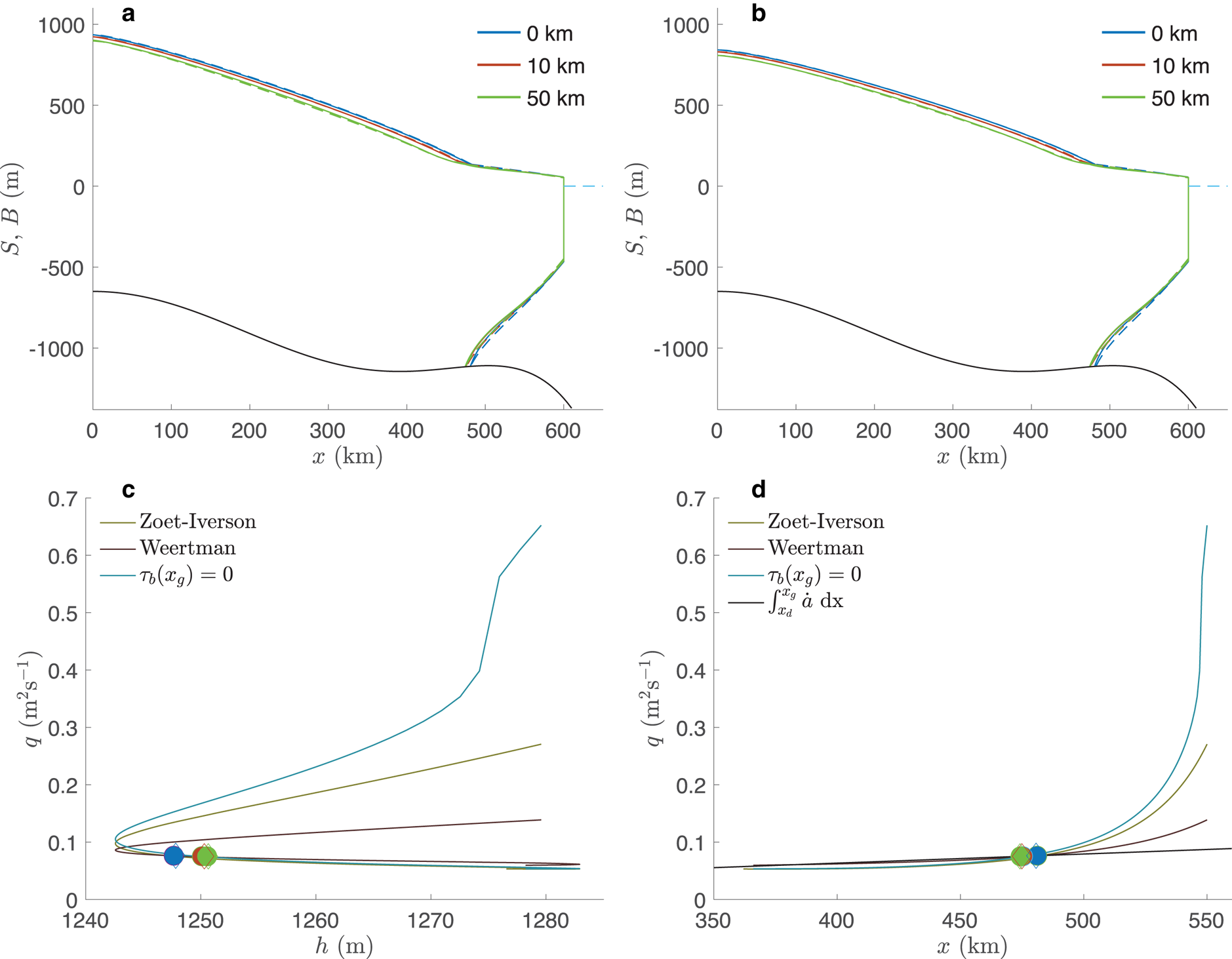
Figure 2. Steady-state configurations of ice sheets. (a) profiles with the Zoet-Iverson sliding law with N reducing to 0 in the 50 km upstream of the grounding line (green line), 10 km (red line) and constant through the length of the ice stream; (b) profiles with the Weertman sliding law with C reducing to 0 in the 50 km upstream of the grounding line (green line), 10 km (red line) and constant through the length of the ice stream. Solid lines are numerical simulations of the full model, dashed lines are results of the approximate model (14). (c) The ice flux at the grounding line as a function of the ice thickness. Lines are solutions of the approximate analytic expression (38a) with the corresponding sliding laws; τ b(x g) = 0 is a solution of (38b); symbols indicate steady-state values from the numerical simulations: filled symbols indicate Zoet-Iverson sliding law open symbols indicate Weertman sliding law, colors indicate the reduction of τ b in the zone upstream of the grounding line similar to those shown in panels (a) and b. (d) The ice flux at the grounding line as a function of the position x g. The light magenta, light green and turquoise lines are solutions of (38a) and (38b), the black line is the integrated accumulation rate through the grounding line (39); symbols are the same as in panel (c).
One of the advantages of the analytic expressions (38) is the possibility to examine the steady-state ice flux for a range of possible grounding line positions, see Figures 2c,d. The solid lines are obtained by solving (38) with the flotation condition (8) for x g between 350 km and 550 km. Due to the appearance of b x and θ in (38), these curves depend on the ice shelf and bed geometry. For $x_g \lesssim$ 350 km all ice on the ice shelf is removed by melting and the ice shelf front is located where the ice thickness goes to zero. We exclude this case from our analysis.
In the presence of a sufficiently long ice shelf (≈100 − 250 km, $x_g\lesssim 475$ km) the form and value of the sliding law do not greatly affect the steady-state ice flux at the grounding line. However, the differences are significantly more pronounced as the ice shelf becomes shorter and buttressing is smaller (Fig. 2(d)).
In steady state, the ice flux at the grounding line matches the integrated surface accumulation (39), and the steady-state grounding line position is determined by the intersection of the flux determined from (38) and the mass balance flux given by (39) (black line in Fig. 2(d)); these intersections are marked by the symbols in Fig. 2(d). The values obtained with the approximate model (14) are in a good agreement with the values obtained in numerical solutions of the full model: the differences between positions obtained with the numerically solved full model (1)–(9) and the roots of (38) are between 650 m a 1200 m for both sliding laws, with smaller values for the configurations with the non-vanishing basal shear and larger values for the configurations for the 50 km reduction zone. The reduction of τ b to zero at the grounding line results in a small reduction (less then 2%) of the steady-state ice flux through the grounding line Figure 2(c)). This reduction is due to the fact the grounding line position is slightly upstream, and in a steady state the flux at the grounding line is the integral of the surface accumulation rate $\dot a$ from the divide to the grounding line; with the constant values of $\dot a$
 , this integral is smaller for the grounding line position located upstream than for the grounding line position located downstream.
As the basal and lateral shear stress depend on the ice velocity, the stability of the steady-state configurations can be determined from (21)–(23). The expressions for the stability coefficients for the Zoet-Iverson sliding law are listed in Appendix B; the expressions for the Weertman sliding law can be found in Haseloff and Sergienko (Reference Haseloff and Sergienko2022)(Eqn. (C20)). According to (22), all configurations shown in Figs. 2(a,b) are stable. This is confirmed with numerical simulations in the same way as in similar studies by Sergienko and Wingham (Reference Sergienko and Wingham2019, Reference Sergienko and Wingham2022) and Sergienko (Reference Sergienko2022b) by displacing the grounding line positions 1 km upstream from their steady-state positions and solving the full time-dependent problem (1)–(8). In all simulations, the displaced grounding lines return to their steady-state positions, confirming that the steady-state configurations are stable.
Expressions (15)–(20) were derived under assumptions that on the grounded part the divergence of the longitudinal stress is smaller than other components of the momentum balance. It is instructive to analyze the components of the ice stream (1a) and ice shelf (1b) momentum balances in order to verify our assumption that for the ice stream the divergence of the longitudinal stress is smaller than other components of the momentum balance is valid. We use the terms from the numerical simulations with the full model (Fig. 3).
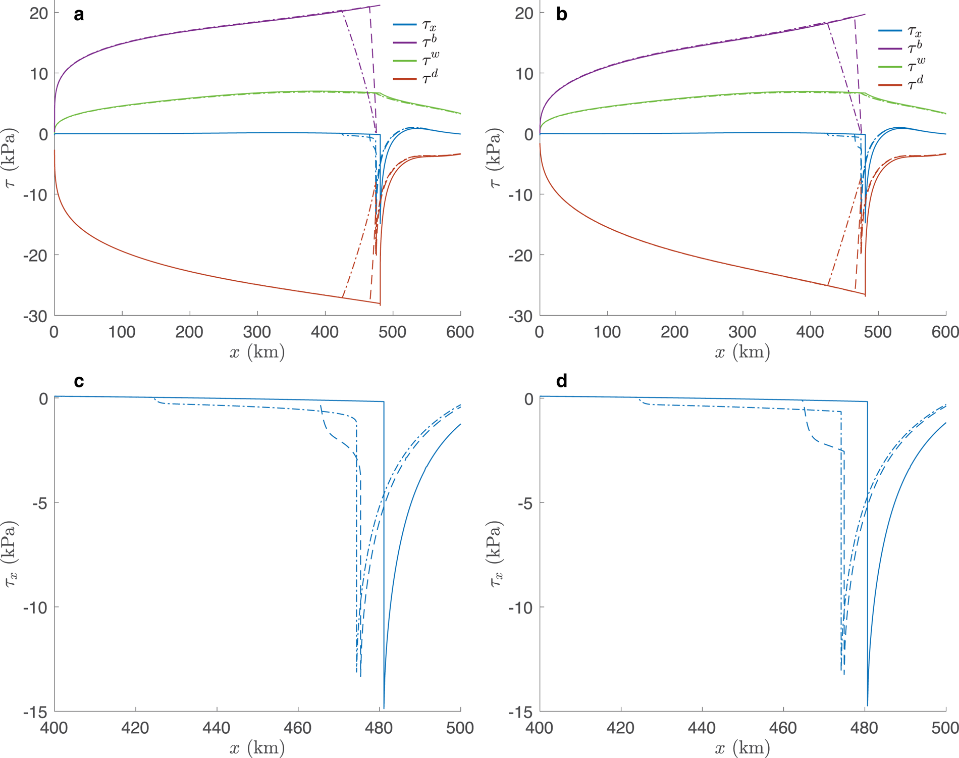
Figure 3. Terms of the steady-state momentum balance. (a) Zoet-Iverson sliding law; solid lines correspond to a constant value of N, dashed lines correspond to reduction of τ b to zero in the 10 km upstream of the grounding line, dotted-dashed lines correspond to reduction of τ b to zero in the 50 km upstream of the grounding line; (b) Weertman sliding law, the lines are the same as in panel (a); (c) zoom-in of τ x terms in the vicinity of the grounding line for Zoet-Iverson sliding law; (d) the same as panel (c) for Weertman sliding law.
The driving stress τ d (last terms on the left-hand side of Eqns. (1a)–(1b)) is discontinuous at the grounding line. This discontinuity results in a discontinuity of the divergence of the longitudinal stress τ x at the grounding line, even though the longitudinal stress itself is continuous in accordance with the continuity condition (7c). The lateral shear stress is continuous at the grounding line because of the continuity conditions (7a)–(7b). As Haseloff and Sergienko (Reference Haseloff and Sergienko2018) surmised, there is a boundary layer downstream of the grounding line, in which the longitudinal stress divergence rapidly reduces to zero, and outside this boundary layer the momentum balance of the ice shelf is between the driving stress and the lateral shear stress.
Upstream of the grounding line, the dominant balance is between the basal shear, lateral shear and driving stress. The imposed reduction of the basal shear is accompanied by the reduction of similar magnitude in the driving stress, rather than significant increase of the magnitude of the longitudinal-stress divergence. It is only in the immediate vicinity of the grounding line that τ x reaches a magnitude of 1–2 kPa, with the value slightly larger for the 10 km reduction zone than for the 50 km reduction zone. This relative smallness of the longitudinal-stress divergence provides justification for the approximated momentum balance (14a). Both sliding laws result in a similar behavior of the stress terms. This behavior of the momentum-balance terms is qualitatively similar to that obtained by Tsai and others (Reference Tsai, Stewart and Thompson2015) in their analysis of an unconfined marine ice sheet with Coulomb sliding law. The linear stability analysis, and hence a derivation of stability conditions of their specific formulation of the sliding law is problematic because it is written in terms of a min function, and its derivatives may not exist.
5. Response to the stochastic variability in submarine melting
While most previous theoretical studies investigate steady-state configurations that assume that all internal and external parameters remain constant in time, realistic ice sheets experience environmental conditions that change in time. This temporal variability happens on a wide range of timescales, because in addition to the long-term changes in the orbital forcing (Milanković, Reference Milanković1941), the Earth's climate has numerous modes of internal variability. Steig and others (Reference Steig, Ding, Battisti and Jenkins2012) linked the variability in the tropical Pacific to variability in submarine melting of the ice shelves in the Pacific region of West Antarctica, and Jenkins and others (Reference Jenkins2018); Christie and others (Reference Christie, Steig, Gourmelen, Tett and Bingham2023) have attributed the grounding line migration of these ice shelves to decadal variability. The results of numerous observational (e.g., Shepherd and others, Reference Shepherd, Wingham and Rignot2004) and modeling (e.g., Cornford and others, Reference Cornford2015; Seroussi and others, Reference Seroussi2017) studies indicate that the grounding-line dynamics is sensitive to submarine melting. Consequently, we chose to explore how the marine ice sheets respond to stochastic variability in submarine melting. Previous modeling studies with idealized (Christian and others, Reference Christian, Robel and Catania2022; Felikson and others, Reference Felikson, Nowicki, Nias, Morlighem and Seroussi2022) and realistic (Hoffman and others, Reference Hoffman, Asay-Davis, Price, Fyke and Perego2019; Robel and others, Reference Robel, Seroussi and Roe2019) geometries show that stochastic variability in the climate forcing have strong effects on the long-term behavior of the grounding lines.
We use the steady-state configurations obtained in the previous section as initial conditions; as discussed above they are all stable configurations. We modify the expression for the submarine melt rate (37) in the following way

where $\Delta \dot m( t)$ varies stochastically

Subscripts s and l refer to ‘short’ and ‘long’ time-scales, $\dot m_{s, l}$ are the amplitudes of the melt-rate variability; T s,l are the correlation time-scales, and ${\cal N}( t)$
 is a noise function with a uniform distribution and zero mean value. For the ‘short’ time-scale we choose the decadal and for the ‘long’ time scale we choose centennial time scales as suggested by in situ and remote sensing observations (Jenkins and others, Reference Jenkins2018; Christie and others, Reference Christie, Steig, Gourmelen, Tett and Bingham2023) and modeling (Latif and others, Reference Latif, Martin and Park2013).
For each sliding law we perform four sets of simulations (see table 2): with constant values of N or C or with a reduction in the 10 km zone upstream of the grounding line; and with T l = 200 yrs or T l = 500 yrs. The values of m s,l are the same in all simulations. Each set consists of five simulations with the noise function ${\cal N}( t)$ initialized with a random seed to ensure independence of the simulation results.
Table 2. Performed time-dependent simulations
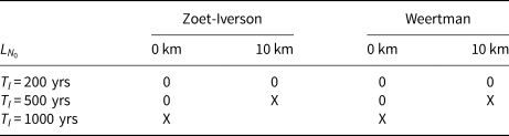
X indicates the occurrence of an irreversible ice sheet collapse, 0 indicates no ice sheet collapse within the 100 kyrs simulation period. For T l = 200 yrs and T l = 500 yrs, 5 simulations were performed for each configuration. Ice sheet collapses occur at different times during these simulations, depending on the seed in the random noise function ${\cal N}$
The problem (1)–(8) is solved numerically on domains with a moving boundary (the grounding line) using an arbitrary Lagrangian-Eulerian (ALE) method (Donea and others, Reference Donea, Huerta, Ponthot and Rodríguez-Ferran2017). The time-step is adaptive and does not exceed two years in order to resolve variability on T s = 10 yrs. The grounding line moves with velocity (17), where all terms are computed by the model and b t = 0. The analysis relies on numerical simulations because it is not possible to write a closed-form expression for θ ((30) is only valid for steady-states). Instead, θ is determined numerically from (10).
Simulations with the Zoet-Iverson sliding law, the 10 km reduction zone and T l=200 yr indicate that stochastic variations in the submarine melting can cause migration of the grounding line on the order of ~40 km with excursions to almost 70 km (Fig. 4(a)). Although the time-averaged values of the rate of the grounding-line migration $\dot x_g$ over the 100 kyr simulation period are low (~−4.5 m yr−1, Fig. 4(b)), there are infrequent instances when the rate of the grounding-line retreat exceeds 1 km yr−1. Together in all five simulations that happened 27 times. The average periodicity of such events is ~18.5 kyr – significantly longer then the long correlation time-scale T l = 200yrs.
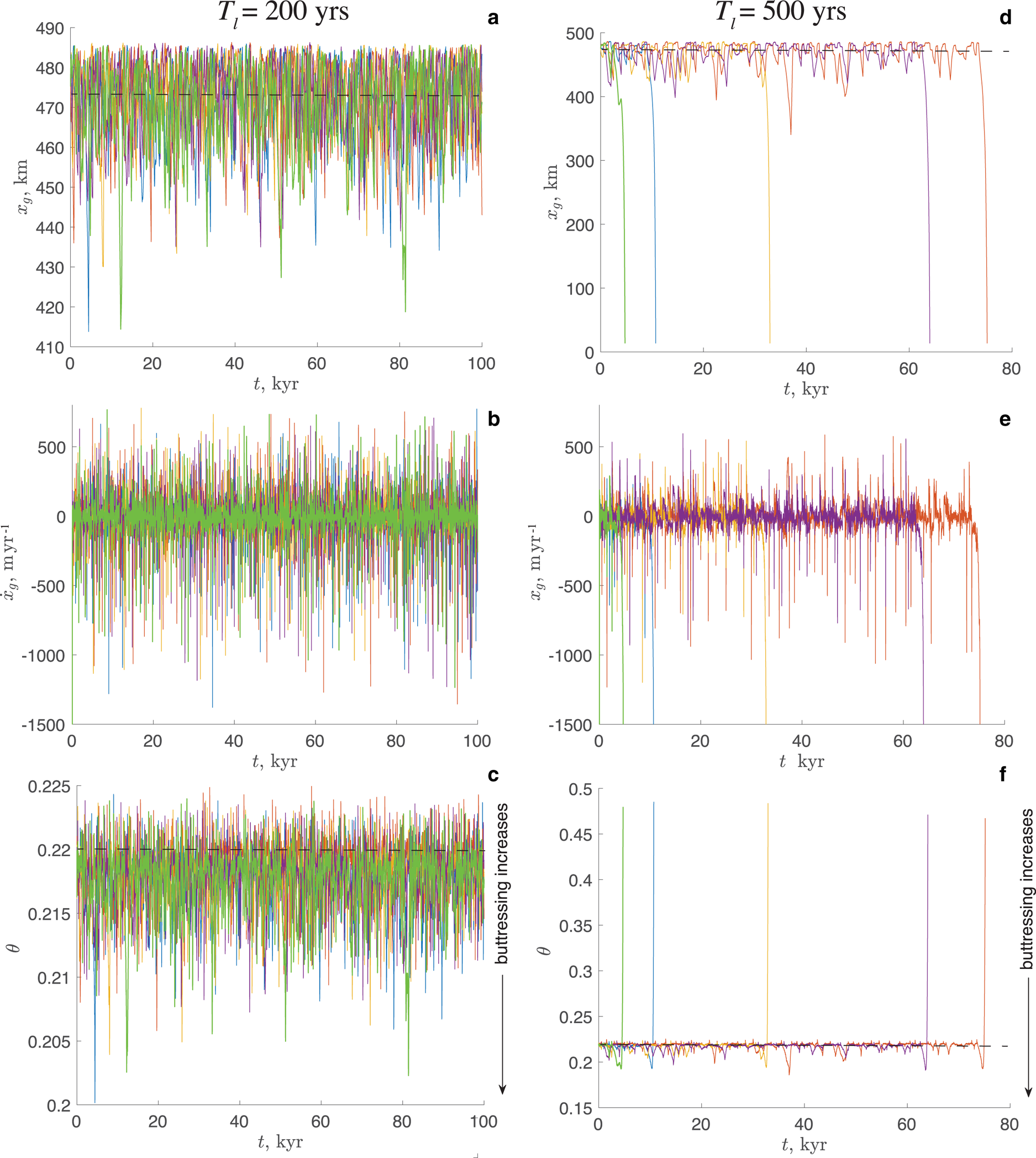
Figure 4. Response of the grounding line to stochastic perturbation in the melt rate with T l = 200 yrs (left column) and T l = 500 yrs for Zoet-Iverson sliding law and with $L_{N_0} = 10$ km. (a) the grounding line position (km); (b) the rate of the grounding line migration (m yr−1); (c) the buttressing parameter θ. Different colors correspond to simulations with different seeds in the noise functions. Dashed lines indicate steady-state values.
In steady state, melting reduces the ice-flux divergence ($\dot a-\dot m = q_x$ ), which can lead to both thinner and slower ice downstream of a melt perturbation. As the steady-state buttressing parameter depends on the integrated ice flux (see (30)), in either case melting leads to a reduction in buttressing if everything else is fixed. In time-dependent calculations as those performed here, melting can either reduce the ice-flux divergence or lead to thinning ($\dot a - \dot m = q_x + h_t$
 ) and it is not obvious how the partition between these two processes affects the buttressing parameter and consequently the grounding line evolution. Moreover, as the location of the calving front is fixed in our simulations, a retreating grounding line lengthens the ice shelf, which could in turn increase the amount of buttressing experienced at the grounding line, with the counter-intuitive result that grounding line retreat and an increase in buttressing go hand-in-hand. This is indeed what we observe: the temporal evolution of the buttressing parameter θ is shown in Figure 4(c) and θ decreases (buttressing increases) as the grounding-line retreats, and conversely. Simulations with the same parameters and no reduction of τ b, as well as simulations with a Weertman sliding law with and without reduction of τ b produce quantitatively similar results.
Increase of the long correlation time-scale T l to 500 yr produces markedly different results in simulations with and without reduction of τ b near the grounding line. If the basal shear stress is reduced at the grounding line ($L_{N_0} = 10$ km) then the marine ice sheet collapses in all simulations, i.e. the grounding line retreats to the ice divide at x d = 0, see Figure 4(d). The timing of this collapse is significantly longer (~5 kyr to ~75 kyr) than the correlation time-scale T l of stochastic variability of submarine melting (500 yr). The rates of grounding line migration prior to the ice-sheet collapse are lower than in simulations with T l =200 yrs. During the collapse they exceed 1 km yr−1 (Fig. 4(e)). Similar to the simulations with the shorter correlation time-scale T l =200 yrs, prior to collapse, the buttressing parameter θ increases when the grounding line retreats, and decreases when the grounding line advances. It is only during the collapse that θ significantly increases indicating strong loss of buttressing (Fig. 4(f)). Simulations with the Weertman sliding law and $L_{N_0} = 10$
 km exhibit quantitatively similar behavior – the ice sheet collapses in ~8 kyr – 120 kyr depending on the simulation.
If τ b does not vanish at the grounding line and T l = 500 yrs, the marine ice sheet does not undergo collapse; instead, it experiences an intermittent advance and retreat of the grounding line. In these simulations, the rate of the grounding line migration is overall lower than in simulations with T l = 200 yr. Only in one simulation (for each sliding law) does the rate of the grounding line migration exceeds 1 km yr−1. However, if the correlation time scale T l is increased to 1000 yrs, then a collapse-like behavior is observed in simulations with both Zoet-Iverson and Weertman sliding laws and constant values of N and C as well. The ice-sheet behaviors in these simulations are similar to those in simulations with τ b vanishing at the grounding line and T l = 500 yrs, described above. Table 2 summarizes these results.
To get a better understanding how the values of the correlation time-scales affect the dynamics of the grounding line, we analyze the co-evolution of the melt rate, the grounding line displacement and the buttressing parameter in single simulations with different values of T l. As Figs. 5(a,b) and 5(d,e) show, in general, the grounding line retreat coincides with a rapid increase of the melt rate and vice versa. Changes in θ overall mimic changes in the grounding-line position: when the grounding line retreats, θ decreases (buttressing increases), and when the grounding line advances, θ increases (buttressing decreases). As pointed out above, this behavior of θ is a consequence of the chosen conditions at the calving front and the fixed values of the surface ablation/accumulation rate $\dot a$ . The difference between simulations with different values of T l is that in simulations with T l = 500 yrs the ice shelf can experience melt rates substantially larger than their mean values for longer time periods compared to simulations with T l = 200 yrs. The longer periods of sustained high melt rates imply longer periods during which the grounding line is upstream of its time-averaged position, and consequently shorter horizontal extent of the grounded part of the ice sheet, through which it accumulates mass.
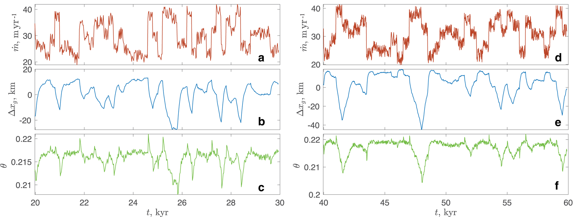
Figure 5. Response of the grounding line to stochastic perturbations in the melt rate in a single simulation for Zoet-Iverson sliding law with the 10 km reduction zone (a)–(c) for T l = 200 yrs and (d)–(f) for T l = 500 yrs. (a), (d) melt rate at the grounding line (m yr−1); (b), (e) displacement of the grounding line from the time-mean position (km); (c), (f) the buttressing parameter θ. Note different horizontal scales in panels (a)–(c) and (d)–(f).
Ultimately, the unstoppable retreat of the grounding line is caused by the loss of the ice flux through the floating ice shelf exceeding the mass gain upstream of the grounding line for prolonged periods of time (Fig. 6). This leads to continuous thinning and further grounding line retreat, until the ice sheet has completely disappeared.
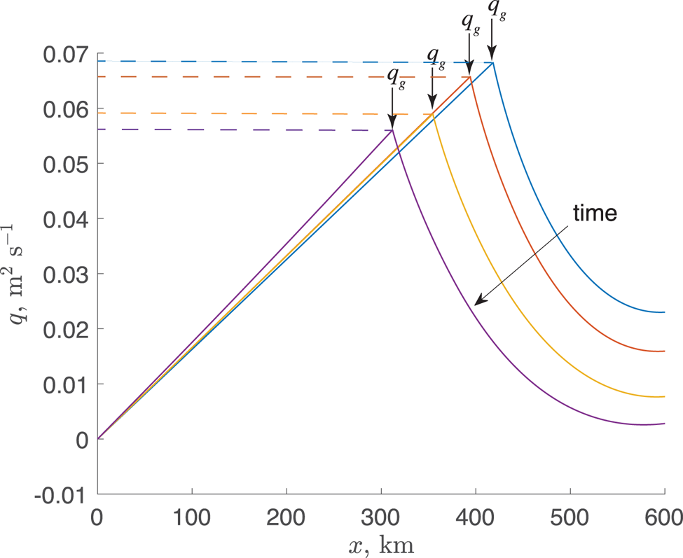
Figure 6. Evolution of the ice flux q(x) through the length of the ice sheet during unstoppable retreat for Zoet-Iverson sliding law with the 10 km reduction zone for T l = 500 yrs. Dashed lines indicate the mass flux gained upstream of the grounded part.
6. Discussion
The existing theoretical analyzes have focused thus far only on steady states of marine ice sheets and their stability. In order to improve our conceptual understanding of the dynamic behavior of marine ice sheets and extend the theoretical analyzes to time-variant behavior that is characteristic of realistic ice sheets experiencing environmental conditions that vary in time, we have developed a framework to analyze the effects of different forms of basal and lateral shear stresses on marine ice sheet dynamics. This framework can be applied to analyze the role of lateral and basal shear stress parameterizations in steady state configurations. Written with general forms of τ w and τ b, the derived expressions also provide insights into how basal and lateral shear (or their absence) affect the temporal evolution of grounding lines. The stability conditions presented here are derived assuming no feedbacks between ice sheet and surface accumulation or submarine melting. Even in the absence of these additional feedbacks, the stability conditions depend on a large number of parameters in a non-trivial fashion. This, and the presence of feedbacks between realistic ice sheets and their environmental conditions, questions generalized statements about their (in)stability and the usefulness of such statements.
The rate of grounding line migration (18) (or (19)) is determined by the imbalance between the stresses on the grounded side of the ice stream (the basal, lateral and form drag associated with the shape of the bed), the ice-shelf buttressing, whose effect is encapsulated in the buttressing parameter θ, the ice velocity at the grounding line, which reflects the effects of lateral and basal shear through the length of the grounded part (19) and the net accumulation/ablation at the grounding line. In steady state these terms balance each other, $\dot x_g = 0$ , and the grounding line does not move. The fact that $\dot x_g$
 is determined by the imbalance of several terms reflects that it is controlled by the competing effects of several processes – both local, at the grounding line, as well as integral, through the lengths of the grounded part and the ice shelf. This indicates that the observed migration of present-day grounding lines cannot be attributed to a single cause (e.g., submarine melting), and all other processes and interactions between them have to be taken into account.
To illustrate the developed framework, we have applied it to a marine ice sheet whose lateral shear increases with velocity and ice thickness and whose basal shear is described by either a Zoet-Iversion sliding law or a Weertman sliding law. The only calving law that yields a steady-state configuration for the chosen bed topography is a fixed calving front position – a widely used condition in idealized and realistic studies. For both sliding laws, we find a good agreement between the steady-state configurations obtained with the full and the approximate models. Analysis of the momentum balances of these ice sheets shows that the divergence of the longitudinal stress at the grounding line is discontinuous (Fig. 3) because the driving stress at the grounding line is discontinuous (Eqn. (1)). Although the discontinuity of the driving stress is obvious from the momentum balance (1), the discontinuity of the divergence of the longitudinal stress is less so. Its existence should be kept in mind in analyzes of the large-scale ice-sheet simulations that are typically based on the vertically integrated momentum balances. Most likely, the requirements of high spatial resolution in the vicinity of the grounding line (Seroussi and others, Reference Seroussi, Morlighem, Larour, Rignot and Khazendar2014; Gladstone and others, Reference Gladstone2017) are associated with the need to resolve this discontinuity of the divergence of the longitudinal stress with sufficient accuracy.
The steady-state configurations with the two sliding laws we compare do not differ qualitatively. There are also no substantial differences in the steady-state configurations of ice sheets whose basal shear reduces to zero or remains large at the grounding line, regardless of the sliding law.
However, if the grounding line is dynamic and driven by stochastic variability in submarine melting, then the ice sheet response depends on the basal shear stress at the grounding line and the magnitude of the correlation time-scales. Our results show that on the given bed topography, the marine ice sheet can exhibit intermittent advance and retreat of their grounding lines in response to up to 40% variations compared to steady-state melt rates if such variations are sustained on the order of 200 yrs. If such melt-rate variations are sustained for longer periods (~500yrs) simulated ice sheets with vanishing basal shear experience unstoppable retreat of their grounding lines, while simulated ice sheets with large basal shear at the grounding lines continue to exhibit intermittent advance and retreat of their grounding lines. They experience such an unstoppable retreat if melt-rate variations are sustained for longer periods (~1 kyr). We point out that the exact values of periods are specific to the chosen parameters - the bed shape, the magnitudes of the basal and lateral shears and the amplitudes of the melt-rate variations. For instance, for the amplitudes of variations much larger than the steady-state values, the correlation timescales may be shorter, e.g., of the order of several decades. However, our finding that for the same amplitudes of the melt-rate variability, the longer correlation timescales can eventually lead to unstoppable retreat of the grounding line is a robust result.
The unstoppable retreat observed in our simulations is a consequence of an excess mass loss at the grounding line which exceeds the integrated mass gain upstream of the grounding line for prolonged periods of time, leading to sustained thinning and retreat of the ice sheet. The retreat occurs at times significantly longer than the stochastic correlation time-scale, on the order of thousands to hundreds of thousands of years, after many periods of melt-rates higher than their time-averaged values. During intermittent grounding-line retreats, the ice-shelf buttressing increases and vice versa. This behavior is a result of holding the calving front position fixed.
Even though our assumption that all parameters except submarine melt rates remain constant in time is unrealistic, it simplifies the analysis and allows us to focus on the effects of time-varying melting. A drastically different response to temporal variability in submarine melting observed in our simulations with vanishing and non-vanishing basal shear stress at the grounding line suggests that the basal traction in the vicinity of the grounding line exhibits a strong control on the transient behavior of marine ice sheets. It also suggests that the temporal variability of basal conditions can have a critical role in its dynamics. Although inferences about the basal shear spatial distribution from surface observations by means of inverse modeling have been done routinely (e.g., Sergienko and others, Reference Sergienko, Bindschadler, Vornberger and MacAyeal2008; Morlighem and others, Reference Morlighem, Seroussi, Larour and Rignot2013), there is very little understanding of its temporal variability. The presence of high basal shear structures in the vicinity of the grounding lines of many Antarctic ice streams and Greenland outlet glaciers has been attributed to the interactions between subglacial hydraulic systems, sediments and the ice flow (Sergienko and Hindmarsh, Reference Sergienko and Hindmarsh2013; Sergienko and others, Reference Sergienko, Creyts and Hindmarsh2014). The highly dynamic nature of the subglacial hydraulic system means that assuming sliding law parameters do not change in time is very limiting. Establishing characteristics of their variability is equally important as establishing a functional form of the sliding law, and is necessary for improvements in understanding of grounding line dynamics.
The concepts of marine ice-sheet stability and instability introduced by Weertman (Reference Weertman1974) and further developed by Schoof (Reference Schoof2007a, Reference Schoof2007b, Reference Schoof2012) apply to steady-state configurations of ice sheets that require that all environmental conditions (in this study expressed via the net surface accumulation/ablation and submarine melting) do not change with time. Neither the present-day ice sheets nor paleo ice sheets have ever attained steady states, because the Earth's climate changes in time on a variety of temporal scales. Hence, the concepts of marine ice-sheet (in)stability cannot be used to describe their behavior. This does not imply, however, that analyzes of steady states are useless. The purpose of such analyzes are different from those focused on the ice-sheets’ response to time-variant environmental conditions (past or future). By ignoring the variability of external conditions, the steady-state analyzes focus on the internal dynamics of the ice sheets and provide insights into their dynamics and conceptual understanding of complex behavior controlled by poorly known subglacial processes, which effects are encapsulated in sliding laws. Additionally, these steady-state analyzes have been a driving force for the development of ice-sheet numerical models, providing benchmarks and establishing the requirements for numerical algorithms and the model resolutions.
Understanding of the behavior of the realistic ice sheets requires analyzes that take into account changing environmental conditions. This requires shifting the focus from steady-state considerations to the temporal evolution of the ice sheets and their characteristics such as the grounding line migration. If its rate is small or close to zero that means that the ice sheets are close or at equilibrium with their environmental conditions; nevertheless, they are not in steady states, because if these conditions change the rate of the grounding line migration changes in response to them (Eqn. (19)). Currently, there is neither quantitative nor conceptual understanding of such dynamic equilibria, their characteristic timescales, controls, etc. Developments of such approaches need to become the focus of future studies.
7. Conclusions
We have developed a generalized framework for the analysis of the steady-state behavior and dynamic evolution of marine ice sheets, and applied it to a configuration with a power-law lateral shear and Zoet-Iversion and Weertman sliding laws. When driven with stochastic variability in submarine melt rates, the grounding line evolution strongly depends on the specific modeling choices (e.g., the size of the modeled domain, the shape of the bed, the conditions at the calving front). Our results illustrate that classifications in stable or unstable grounding lines are not useful concepts in understanding the transient behavior of ice sheets. Although all our simulations started from stable steady-state configurations, their response to temporal variability, even of a stochastic nature with no trends, cannot be described in terms of ‘stable’ or ‘unstable’ at any given time. Understanding the dynamic behavior of marine ice sheets requires a new conceptual approach that takes into account the ice-sheet environmental conditions and their variability on a wide range of temporal scales.
Code availability
Numerical models used in this study are available on Zenodo https://zenodo.org/record/7637662 (Sergienko and Haseloff, Reference Sergienko and Haseloff2023).
Acknowledgements
We would like to thank Scientific Editor Jonathan Kingslake and two anonymous referees for their useful suggestions that greatly improved readability of the manuscript. This study was supported by an award NSF2218463 from the National Science Foundation (M. H.) and an award NA18OAR4320123 from the National Oceanic and Atmospheric Administration, U.S. Department of Commerce (O. S.). The statements, findings, conclusions, and recommendations are those of the author and do not necessarily reflect the views of the National Oceanic and Atmospheric Administration, or the U.S. Department of Commerce.
Appendix A. Stability analysis of steady-state configurations
Here, we describe details of a linear stability analysis of an approximate problem (14). As usual, we consider small perturbations around the steady state

where steady-state solutions are denoted by $\hat { }$ , perturbation solutions are denote by $\tilde { }$
 , and σ is a small parameter. Substituting these expressions to (14) and collecting terms in the lowest order of σ lead to the perturbation problem


where


ξ ={ξ b, ξ w} represents all variables that τ b and τ w on the grounded, ice-stream side described by (4) depend on; $\varpi = \left\{\xi ,\; \, \dot m,\; \, x_c\ldots \right\}$ represents all variables that τ w on the floating, ice-shelf side and θ depend on; and variable subscripts (x, t, h, q, $\varpi$
 ) indicate a partial derivative with respect to the respective variable.
Taking into account the steady-state momentum balance (12a), the perturbation momentum balance (A.2a) can be written as

Substitution of this expression to the perturbation mass balance (A.2b) gives

This is a second-order PDE for $\tilde h$ . Its solution can be written in a form

Substitution this form to (A.5) transforms the perturbation problem (A.2) into an eigenvalue problem with λ being an eigenvalue


where


and


were taken into account.
The eigenvalue problem (A.7) is of the same kind as those considered by Sergienko and Wingham (Reference Sergienko and Wingham2022); Haseloff and Sergienko (Reference Haseloff and Sergienko2022). Similar to these and Schoof's(Reference Schoof2012) analysis, it is possible to put (A.7) into Sturm-Liouville form. As in these previous studies, it is not possible to write a closed form expression for λ. It is possible, however, to establish conditions under which all eigenvalues are negative, implying that a steady-state configuration is stable. According to theorem 1 of Linden (Reference Linden1991), the eigenfunction corresponding to the largest eigenvalue does not have zeros if the term in parenthesis of the first square brackets on the left-hand side of (A.7c), $\displaystyle {( G_1( \hat \xi ) + G_2( \hat \xi ) \hat q-F_1( \varpi ) \theta _q( \hat \varpi ) ) }$ , is positive. If this condition is satisfied, the term $\displaystyle {{ { \int } _0^{\hat {\hskip1pt x}_g}\tilde h{\rm d}x}/{\tilde h( \hat x_g) }}$
 is positive. Consequently, the first square bracket on the left-hand side of (A.7c) is positive. The second square bracket has to be negative in order for the ice stream remain grounded (Schoof, Reference Schoof2012). Thus, the sign of λ and stability of a steady state is determined by the sign of the right-hand side of (A.7c). It is stable if

If the inequality sign is reversed, the steady state is unstable.
If τ b and τ w do not depend on u, it is possible to compute the term $\displaystyle {{ { \int } _0^{\hat {\hskip1pt x}_g}\tilde h{\rm d}x}/{\tilde h( \hat x_g) }}$ in the square brackets of the left-hand side of (A.7c). With all other terms known, this expression (A.7c) allows to determine the eigenvalue λ. This can be achieved by observing that the term (τ w + τ b)q in (A.2a) is zero. Taking into account the steady-state momentum balance (12a) and rearranging terms, (A.2a) gives

Integrating both sides of this expression leads to the following expression for $\tilde h( x)$

where C 0 is a constant of integration. Using this expression leads to

Rearranging terms in (A.7c), one obtains

where the term $\displaystyle {{ { \int } _0^{\hat {\hskip1pt x}_g}\tilde h{\rm d}x}/{\tilde h( \hat x_g) }}$ is defined by (A.14).
Stability conditions in terms of the flux gradient
The above stability conditions can be written in terms of the gradient of the ice flux at the grounding line $\displaystyle {{{\rm d} q_g}/{{\rm d} x_g}}$ , a form used by Schoof (Reference Schoof2012). To do so we write the ice-flux expression (15) as an implicit function F

where the ( ⋅ ) placeholder indicates dependencies on other variables than (q, q x, h, x). The perturbation stress condition (A.2c) becomes

Variable subscripts (x, t, h, q, q x) indicate a partial derivative with respect to the respective variable. Note that we expect τ w, τ b and θ to depend on different combinations of h, q, x, (Eqn. (A.3)).
In this form, the eigenvalue problem similar to that described by Eqn. (A.7c) becomes


and the stability conditions are

We can identify $\hat q_x = \dot a$ , b x/(1 − δ) = −dh g/dx g, and $\hat q_{xx} = {\rm d} \dot a/ {\rm d} x_g$
 at the grounding line $x = \hat x_g$
 , i.e.

If the inequality sign is reversed, the steady state is unstable. To understand this expression, we take the derivative of $F( q_g,\; \, \dot a,\; \, h_g,\; \, x_g,\; \, \cdot )$ with respect with x g:

which leads to

We have already required F q > 0 above, so the stability condition is

In the case of τ b and τ w being independent of u, the corresponding expression for λ is

Appendix B. Linear stability analysis for a power-law lateral shear and zoet-iverson sliding law
Here we provide specific forms of the coefficients in the stability conditions (21)–(22).


The terms in Eqn. (B.1c) are


where $\displaystyle {\alpha = {N_f}/{2 + N_fk}( {1}/{\eta ( Ra) ^2k_0^3} + {4C_1}/{( Ra) ^2k_0}) }$ ; N h = ρg − ∂hp w and ∂hp w is a derivative of p w with respect to the ice thickness h.
The terms θ h,θ q and $\theta _{\varpi ( \varpi \neq h) }\varpi _x = \theta _qq_x + \theta _{x_c}\partial _xx_c$ in (22) are the following


where


In the example considered here, x c is prescribed, and $\theta _{x_c} = 0$ , ∂xx c = 0.


 Open access