


1. Introduction
Inertial waves are propagating disturbances in rotating flows, where the Coriolis force provides the restoring mechanism (Greenspan Reference Greenspan1968; Pedlosky et al. Reference Pedlosky1987). They occur at frequencies ranging from zero to the Coriolis frequency, and are of dynamical significance in several natural systems where the background rotation is important, such as the Earth's core (Aldridge & Lumb Reference Aldridge and Lumb1987), ocean (Fu Reference Fu1981) and atmosphere (Zhang & Yi Reference Zhang and Yi2007), as well as astrophysical flows (Ogilvie & Lin Reference Ogilvie and Lin2007; Favier et al. Reference Favier, Barker, Baruteau and Ogilvie2014; Ouazzani et al. Reference Ouazzani, Lignières, Dupret, Salmon, Ballot, Christophe and Takata2020). Owing to their ability to transport significant momentum and energy across large distances, inertial waves are of importance in overall energy budgets and dynamical studies of the aforementioned natural systems. As a result, inertial wave generation and dissipation have been topics of several studies in the literature. One of the pathways for inertial wave dissipation is linear instability, which represents the focus of the current study.
Inertial wave dynamics has been studied both theoretically and experimentally in the last few decades. Early experimental studies were performed in finite-sized, closed rotating cylindrical tanks, where linear and nonlinear regimes of inertial wave modes were investigated (Greenspan Reference Greenspan1969; McEwan Reference McEwan1970; Manasseh Reference Manasseh1992; Kobine Reference Kobine1995). In these studies, nonlinear wave interactions, along with viscous boundary layer dynamics, were shown to play an important role in the associated mean circulation and breakdown of inertial waves into small-scale disorder. To understand these experimental observations, Kerswell (Reference Kerswell1999) performed a linear stability analysis of two representative inertial wave modes in confined cylindrical geometry to conclude that triadic resonances constitute the generic mechanism for secondary instability in rapidly rotating fluids. Motivated by applications in the Earth's core and tidally excited astrophysical bodies, inertial wave instabilities and associated mean flow dynamics have also been studied in spherical shells with precession and differential rotation (Lorenzani & Tilgner Reference Lorenzani and Tilgner2003; Wicht Reference Wicht2014; Hoff, Harlander & Egbers Reference Hoff, Harlander and Egbers2016a; Hoff, Harlander & Triana Reference Hoff, Harlander and Triana2016b).
Our current study is motivated by inertial wave dynamics in the ocean, where a Cartesian geometry is suitable for describing processes that do not span several degrees in latitude or longitude. The primary source of inertial waves in the ocean is the winds, and it is now recognized that the energy input into wind-driven inertial waves with frequencies close to the local Coriolis frequency is comparable to the energy input into internal tides (Alford et al. Reference Alford, MacKinnon, Simmons and Nash2016). Specifically, wind stress changes excite motions at frequencies close to the Coriolis frequency in the upper ocean, which could subsequently propagate as inertial waves. In addition, internal gravity waves excited by other mechanisms, such as tide–topography (Garrett & Kunze Reference Garrett and Kunze2007) and flow–topography (Nikurashin & Ferrari Reference Nikurashin and Ferrari2010; Zemskova & Grisouard Reference Zemskova and Grisouard2021) interactions, can also be significantly influenced by the background rotation and hence inertial wave dynamics (MacKinnon & Winters Reference MacKinnon and Winters2005).
One of the often-studied instability mechanisms in internal waves is the triadic resonance instability (TRI), where secondary waves with frequencies  $\omega _1 \text{ and } \omega _2$ and wavevectors
  ${\boldsymbol k_1} \text{ and }{\boldsymbol k_2}$ are excited, following
  $\omega _1+\omega _2 = n\omega$ and
  ${\boldsymbol k_1}+{\boldsymbol k_2} = n{\boldsymbol k}$ (Drazin Reference Drazin1977). Here,
  $\omega$ and
  ${\boldsymbol k}$ are the primary wave frequency and wavevector, respectively, and
  $n+1$ is the order of resonance (in the primary wave amplitude). A special case of TRI is the parametric subharmonic instability (PSI), where
  $n=1$,
  $\omega _1 = \omega _2 = \omega /2$ and
  ${\boldsymbol k_1} = -{\boldsymbol k_2}$ with
  $|{\boldsymbol k_1}|\gg |{\boldsymbol k}|$ (Staquet & Sommeria Reference Staquet and Sommeria2002). Recognizing that PSI is not well-understood in inertial waves, Bordes et al. (Reference Bordes, Moisy, Dauxois and Cortet2012) studied the evolution of secondary subharmonic waves in inertial waves excited by a wave generator at laboratory scale. While triadic resonance was found to be the relevant mechanism of instability, viscous effects were shown to be important in the selection of secondary waves at the laboratory scale. In a more recent study, Mora et al. (Reference Mora, Monsalve, Brunet, Dauxois and Cortet2021) showed that the subharmonic waves produced by TRI do not propagate in the same vertical plane as the base inertial wave, thus establishing the three-dimensional (3-D) nature of TRI even at small primary wave amplitudes. Using classical triadic resonance equations for small primary wave amplitudes, Mora et al. (Reference Mora, Monsalve, Brunet, Dauxois and Cortet2021) elucidated the 3-D nature of TRI in inertial waves. In this study, we perform a linear stability analysis of plane inertial waves using the local stability approach.
While Floquet theory has previously been used to study linear instabilities in spatially and temporally periodic internal waves (Mied Reference Mied1976; Drazin Reference Drazin1977; Klostermeyer Reference Klostermeyer1982; Sonmor & Klaassen Reference Sonmor and Klaassen1997), the local stability approach is computationally efficient in exploring a wider range of base flow and perturbation parameters, and thereby identifying different instability mechanisms in various parameter regimes (Ghaemsaidi & Mathur Reference Ghaemsaidi and Mathur2019). The local stability analysis (Lifschitz & Hameiri Reference Lifschitz and Hameiri1991) considers the evolution of short-wavelength perturbations, for which the linear stability equations reduce to a set of ordinary differential equations that govern the evolution of the perturbation amplitude and wavevector along fluid particle trajectories in the base flow. It has been extensively used to investigate various instabilities in idealized models of vortices (Bayly Reference Bayly1986; Leblanc Reference Leblanc1997; Sipp & Jacquin Reference Sipp and Jacquin2000), including the effects of background rotation (Godeferd, Cambon & Leblanc Reference Godeferd, Cambon and Leblanc2001) and stratification (Miyazaki & Fukumoto Reference Miyazaki and Fukumoto1992; Aravind, Mathur & Dubos Reference Aravind, Mathur and Dubos2017).
The local stability approach has been used to study linear instabilities in waves too, with examples including Gerstner's waves (Leblanc Reference Leblanc2004), equatorially trapped waves (Constantin & Germain Reference Constantin and Germain2013) and edge waves on a sloping beach (Ionescu-Kruse Reference Ionescu-Kruse2014). In the domain of internal waves in Cartesian geometry, it has been used to study standing inertial waves (Lifschitz & Fabijonas Reference Lifschitz and Fabijonas1996), plane internal gravity waves (Ghaemsaidi & Mathur Reference Ghaemsaidi and Mathur2019), and standing and propagating inertia-gravity waves (Miyazaki & Adachi Reference Miyazaki and Adachi1998). For standing inertial waves, Lifschitz & Fabijonas (Reference Lifschitz and Fabijonas1996) demonstrated that the growth rate tends to infinity as the amplitude and spatial scale of the inertial wave increases and decreases, respectively. In contrast to classical triadic resonance calculations, a linear stability analysis based on the local stability approach does not assume any specific instability mechanism; rather, instabilities such as TRI emerge as an outcome of the analysis. Furthermore, the linear stability analysis makes no assumptions about the amplitude of the base flow inertial wave, thus going beyond the small-amplitude inertial wave regime. Unlike the classical triadic resonance calculations, however, the local stability approach neglects the finite-wavenumber and viscous effects in the perturbations.
In the current study, we perform a local stability analysis of plane inertial waves to investigate linear instabilities associated with 3-D, short-wavelength perturbations. In addition to augmenting our understanding of previously observed characteristics of TRI in inertial waves, our study also explores the entire four-dimensional space occupied by inertial wave and perturbation parameters. Specifically, we obtain instability characteristics as a function of inertial wave amplitude/orientation and the orientation of the perturbation wavevector. The rest of the paper is organized as follows. Section 2 describes the base inertial wave and the local stability equations. Section 3 presents the growth rate variation as a function of various base flow and perturbation parameters, followed by an identification of various instability mechanisms in different regions of the parameter space. Section 4 summarizes the results and concludes with a discussion of the future scope of our study.
2. Theory
For an inviscid, incompressible flow with a uniform density  $\rho _0$, the governing equations of motion in a rotating frame of reference are (Pedlosky et al. Reference Pedlosky1987)
 $$\begin{gather} \boldsymbol{\nabla}\boldsymbol{\cdot}\boldsymbol{U}=0, \end{gather}$$
 $$\begin{gather}\boldsymbol{U_t}+\boldsymbol{U} \boldsymbol{\cdot}\boldsymbol{\nabla} \boldsymbol{U}+2\boldsymbol{\varOmega}\times\boldsymbol{U}={-} \boldsymbol{\nabla}(p/\rho_0)-g\hat{\boldsymbol e}_{\boldsymbol z}, \end{gather}$$
where  ${\boldsymbol U}$ and
  $p$ are the total velocity and pressure fields, respectively. Here
  ${\boldsymbol \varOmega }$ is the constant background rotation, which we assume in this study to be
  ${\boldsymbol \varOmega } = (f/2)\hat {\boldsymbol e}_{\boldsymbol z}$. The acceleration due to gravity is
  $g$, which acts along
  $-\hat {\boldsymbol e}_{\boldsymbol z}$. Decomposing the total flow into a base flow and a perturbation field (denoted by a prime), we write
 $$\begin{gather} \boldsymbol{U}=\bar{u}+ u', \end{gather}$$
 $$\begin{gather}p={-}\rho_0gz+\bar{p}+p', \end{gather}$$
where the base flow is assumed to be a combination of quiescent flow with a hydrostatic pressure distribution and a plane inertial wave. Specifically, the velocity and pressure fields  $\bar {\boldsymbol u}$ and
  $\bar {p}$ are described by a plane inertial wave, as discussed in § 2.1.
2.1. Plane inertial wave
A plane inertial wave, whose instability characteristics we study, can be described by
 $$\begin{gather} \bar{\psi}=\varPsi \cos(kx+mz-\omega t), \end{gather}$$
 $$\begin{gather}\bar{p}={-\rho_0 \omega }\varPsi\cot\varPhi \sin(kx+mz-\omega t), \end{gather}$$
 $$\begin{gather}\bar{v}={-}\frac{f\varPsi m}{\omega}\cos(kx+mz-\omega t), \end{gather}$$
where the stream function  $\bar {\psi }$ specifies the horizontal and vertical velocity components as
  $(\bar {u},\bar {w}) = (-\partial \bar {\psi }/\partial z,\partial \bar {\psi }/\partial x)$,
  $\bar {v}$ is the out-of-plane velocity component along the
  $y$-axis and
  $\bar {p}$ is the corresponding pressure field. Here
  $\varPsi$ is the stream function amplitude, and
  $\varPhi$ represents the angle that the wavevector
  ${\boldsymbol k}=k{\boldsymbol e_x}+m{\boldsymbol e_z}$ makes with the
  $x$-axis. Based on the orthogonality between the phase and group velocities for a plane inertial wave,
  $\varPhi$ can also be thought of as the angle made by the energy propagation direction with the vertical
  $z$-axis. We note here that the underlying mechanism that generates the plane inertial wave in (2.5)–(2.7) is not considered in the base flow for the stability analysis.
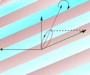
A schematic of the plane inertial wave is shown in figure 1. The wavenumbers  $(k,m)$ and the frequency
  $\omega$ are related by the dispersion relation (Greenspan Reference Greenspan1968)
 \begin{equation} \sin^2\varPhi=\frac{m^2}{k^2+m^2}=\frac{\omega^2}{f^2}. \end{equation}
As  $\omega$ increases from zero to
  $f$,
$f$,  $\varPhi$ increases from
  $0^\circ$ to
  $90^\circ$. It is worth clarifying that the
  $\omega = f$ limit is referred to as the inertial wave in oceanography (Kunze & Sanford Reference Kunze and Sanford1984), whereas we refer to the entire range of
  $0\le \omega \le f$ as inertial waves. Choosing
  $f^{-1}$ and
  $|{\boldsymbol k}|^{-1}$ as representative time and length scales, respectively, we define the following dimensionless parameters to characterize the base flow:
 \begin{equation} A=\frac{|{\boldsymbol k}|^2\varPsi}{f}, \quad \varPhi=\tan^{{-}1}\left(\frac{m}{k}\right), \end{equation}
where  $A$ and
  $\varPhi$ are dimensionless parameters that characterize the inertial wave velocity amplitude and orientation, respectively. It is noteworthy that
  $A$ is a Rossby number that represents the ratio between the internal wave shear in the
  $x$–
$x$– $z$ plane and the background rotation. In terms of the energy propagation direction (aligned with the group velocity vector,
  ${\boldsymbol c_g}$, shown in figure 1), smaller values of
  $\varPhi$ correspond to steeper inertial waves. The corresponding non-dimensional velocity components in the
  $x$–
$x$– $z$ plane are
 \begin{equation} (\bar{u},\bar{w})=A\sin({x}\cos\varPhi +{z}\sin\varPhi -{t}\sin\varPhi )(\sin\varPhi,-\cos\varPhi). \end{equation}
In the rest of this paper, all the variables are non-dimensional. It is worth noting that the plane inertial wave in (2.5)–(2.7) is a solution of the fully nonlinear inviscid equations of motion (Craik & Criminale Reference Craik and Criminale1986), thus rendering our stability analysis valid even for finite-amplitude inertial waves.

Figure 1. (a) Schematic depiction of the plane inertial wave with a wavevector  ${\boldsymbol k}$ which is aligned at an angle
  $\varPhi$ with the
  $x$-axis. The background is
  ${\boldsymbol \varOmega } = f/2 {\boldsymbol e_z}$. The projections of a representative fluid particle trajectory (not drawn to scale) on the
  $y$–
$y$– $z$ and
  $x$–
$x$– $z$ planes are shown in red and green, respectively. The initial perturbation wavevector
  $\kappa _0$ is aligned at an angle
  $\theta _0$ with the
  $x$–
$x$– $z$ plane. The projection of
  $\kappa _0$ on the
  $x$–
$x$– $z$ plane makes an angle
  $\phi _0$ with the
  $x$-axis. The projections of the representative fluid particle trajectory are also shown in panels(b) and (c).
2.2. Local stability equations
Following Lifschitz & Hameiri (Reference Lifschitz and Hameiri1991), we write short-wavelength perturbations, which we superimpose onto the base flow, in the Wentzel–Kramers–Brillouin–Jeffreys form
 \begin{equation} (\boldsymbol{u'},p')=\exp({\rm i}\varTheta/\epsilon)[(\boldsymbol{a},p) +\epsilon(\boldsymbol{a}_\epsilon,p_\epsilon)+\cdots], \end{equation}
where  $a({\boldsymbol {x},t}) \text{ and } p({\boldsymbol {x},t})$ are, respectively, the complex leading-order velocity and pressure perturbation amplitudes. Here
  $\varTheta (x,t)$ is a real-valued phase function and
  $\epsilon$ is a small parameter representative of the ratio between the perturbation and the base flow inertial wavelength scales. Here
  $\boldsymbol {\kappa }{ ({\boldsymbol x},t)}=\boldsymbol {\nabla } \varTheta /\epsilon$ is the perturbation wavevector, which corresponds to short-wavelength perturbations owing to
  $\epsilon \ll 1$. Substituting equation (2.11) into (2.1) and (2.2) and gathering terms at
  $O(\epsilon ^{-1})$ and
  $O(\epsilon ^0)$, we obtain the local stability equations as (Godeferd et al. Reference Godeferd, Cambon and Leblanc2001; Nagarathinam, Sameen & Mathur Reference Nagarathinam, Sameen and Mathur2015)
 $$\begin{gather} \frac{{\rm d} {\boldsymbol{\kappa}}}{{\rm d} t}={-}(\boldsymbol{\nabla} \boldsymbol{\bar{u}})^{\rm T}\boldsymbol{\cdot} \boldsymbol{\kappa}, \end{gather}$$
 $$\begin{gather}\frac{{\rm d} \boldsymbol{a}}{{\rm d} t}={-}\boldsymbol{\nabla}\boldsymbol{\bar{u}}\boldsymbol{\cdot} \boldsymbol{a}-\hat{\boldsymbol e}_{\boldsymbol z}\times\boldsymbol{a}+ \frac{\boldsymbol{\kappa}}{|\boldsymbol{\kappa}|^2}[2(\boldsymbol{\nabla} \boldsymbol{\bar{u}}\boldsymbol{\cdot}\boldsymbol{a})\boldsymbol{\cdot}\boldsymbol{\kappa}+ (\hat{\boldsymbol e}_{\boldsymbol z}\times\boldsymbol{a})\boldsymbol{\cdot}\boldsymbol{\kappa}], \end{gather}$$
where  ${\rm d}/{\rm d}t = \partial /\partial t + {\bar {\boldsymbol u}}\boldsymbol {\cdot }\boldsymbol {\nabla }$ is the material time derivative along fluid particle trajectories in the base flow. Equations (2.12) and (2.13) represent the evolution of the perturbation wavevector and leading-order velocity perturbation amplitude along fluid particle trajectories in the base flow
  ${\bar {\boldsymbol u}}$.
2.2.1. Solution along an inertial wave trajectory
In this subsection, we present analytical expressions for fluid particle trajectories in a plane inertial wave and discuss how to obtain solutions of (2.12) and (2.13) along specific fluid particle trajectories.
Defining  ${\beta }={z_0}\sin \varPhi +{x_0}\cos \varPhi$, where
  $(x_0,z_0)$ is the initial position, the fluid particle trajectory
  ${\bar {\boldsymbol x}}(t) = (\bar {x}(t),\bar {y}(t),\bar {z}(t))$ in the plane inertial wave (2.10) is
 $$\begin{gather} [{\bar{x}(t)},{\bar{z}(t)}]=[x_0,z_0]+A[\cos({\beta}-{t}\sin\varPhi)- \cos{\beta},-\cot\varPhi(\cos({\beta}-{t}\sin\varPhi)-\cos{\beta})], \end{gather}$$
 $$\begin{gather}{\bar{y}(t)}={\frac{A}{\sin\varPhi}}(\sin({\beta}-{t}\sin\varPhi)-\sin{\beta}). \end{gather}$$
Along the specific fluid particle trajectories represented by (2.14a,b), (2.12) and (2.13) reduce to ordinary differential equations with the dependent variables  $\boldsymbol {\kappa }$ and
  $a$ parameterized in terms of the only independent variable
  $t$.
$t$.
Substituting equations (2.14a,b) and defining  $\alpha ={\kappa _{x0}}\sin \varPhi -{\kappa _{z0}}\cos \varPhi$, the solution of (2.12) is
 \begin{align}
{\boldsymbol{\kappa}(\bar{\boldsymbol{x}}(\boldsymbol{t}),t)}&=
{\boldsymbol{\kappa_0}}+A\{\alpha(\sin({\beta}-{t}\sin\varPhi)-
\sin{\beta})\nonumber\\
& +\kappa_{y0}(\cos{\beta}-\cos({\beta}-
{t}\sin\varPhi))\}[\cot\varPhi,0,1],
\end{align}
\begin{align}
{\boldsymbol{\kappa}(\bar{\boldsymbol{x}}(\boldsymbol{t}),t)}&=
{\boldsymbol{\kappa_0}}+A\{\alpha(\sin({\beta}-{t}\sin\varPhi)-
\sin{\beta})\nonumber\\
& +\kappa_{y0}(\cos{\beta}-\cos({\beta}-
{t}\sin\varPhi))\}[\cot\varPhi,0,1],
\end{align}where
 \begin{equation} {\boldsymbol{\kappa_0}}=[\kappa_{x0},\kappa_{y0},\kappa_{z0}]= [\cos\theta_0\cos\phi_0,\sin\theta_0,\cos\theta_0\sin\phi_0], \end{equation}
is the initial perturbation wavevector. Here,  $\theta _0$ is the angle made by
  $\kappa _0$ with its projection on the
  $(x,z)$ plane, and
  $\phi _0$ is the angle that the projection of
  $\boldsymbol {\kappa _0}$ on the
  $(x,z)$ plane makes with the
  $x$-axis. These angles are geometrically depicted in figure 1. Owing to the invariance of (2.12) and (2.13) with respect to a scaling of
  $\boldsymbol {\kappa }$ with any scalar, it suffices to consider initial perturbation wavevectors of unit magnitude (see (2.16)).
To obtain the growth rates for perturbations in a plane inertial wave of given  $(A,\varPhi )$, (2.13) is solved numerically for different values of
  $(\theta _0,\phi _0)$ in the range of
  $\theta _0\in [-90^\circ,90^\circ ]$ and
  $\phi _0\in [0^\circ,180^\circ ]$. Integrating equation (2.13) for three different initial conditions, namely
  $a_{01} = [1,0,0], a_{02}=[0,1,0] \text{ and } a_{03}=[0,0,1]$, Floquet theory is invoked to estimate the growth rate as
 \begin{equation} \sigma=\frac{\max({\rm Re}(\log(\textrm{eigenvalues of }{{\boldsymbol M}})))}{2{\rm \pi}/ \sin\varPhi}, \end{equation}
where  ${\boldsymbol M}=[a_{1};a_{2};a_{3}]$. Here,
  $a_1, a_2$ and
  $a_3$ are the amplitude vectors obtained upon integrating equation (2.13) for one inertial wave time period
  $T = 2{\rm \pi} /\sin \varPhi$, using the initial conditions
  $a_{01}, a_{02}$ and
  $a_{03}$, respectively. For the numerical integration of (2.13), the Runge–Kutta fourth-order scheme was used with a time step of
  $\delta t = T/1000$. This choice for
  $\delta t$ ensured that the growth rates changed by less than
  $1\,\%$ when
  $\delta t$ is halved. Finally, for a given
  $(A,\varPhi )$, growth rates were calculated on an equispaced grid of 500 by 500 points on the
  $(\phi _0,\theta _0)$ plane. The maximum growth rate on the
  $(\phi _0,\theta _0)$ plane is denoted by
  $\sigma ^*$, and the corresponding location is referred to as
  $(\phi _0^*,\theta _0^*)$.
3. Results
We begin this section with results on the growth rate distributions in the parameter space of perturbation characteristics (§ 3.1). The growth rates at low and moderate inertial wave amplitudes are discussed within the context of PSI in § 3.2. Finally, in § 3.3, the dominant instability characteristics are presented and discussed.
3.1. Growth rate distribution
In figure 2, we present the growth rate  $\sigma$ on the (
 $\phi _0,\theta _0$) plane for nine different pairs of base flow parameters (
 $A,\varPhi$). The growth rate is periodic in
  $\phi _0$ upon a flip in
  $\theta _0$ such that
  $\sigma (\phi _0,\theta _0) = \sigma (180^\circ +\phi _0,-\theta _0)$. Interestingly, unlike for an internal wave with no background rotation (Ghaemsaidi & Mathur Reference Ghaemsaidi and Mathur2019),
  $\sigma$ is not symmetric about
  $\theta _0 = 0$ for an inertial wave. The loss in symmetry can be understood as a consequence of the background rotation, as a result of which (2.12) and (2.13) are not invariant when
  $\theta _0$ is replaced with
  $-\theta _0$. Specifically, it is already evident in the analytical solution for
  $\kappa$ (see (2.15)) that replacing
  $\kappa _{y0}$ with
  $-\kappa _{y0}$ non-trivially changes the evolution of
  $\kappa _x$ and
  $\kappa _y$, and hence that of the perturbation wavevector orientation also. In figure 2, while the inertial wave amplitude varies from
  $A = 0.1$ to 1 to 10 from figure 2(a–c) to figure 2(d–f) to figure 2(g–i), the inertial wave orientation
  $\varPhi$ varies from
  $15^{\circ }$ to
  $45^{\circ }$ to
  $75^{\circ }$ from figure 2(a,d,g) to figure 2(b,e,h) to figure 2(c, f,i).

Figure 2. Growth rate  $(\sigma )$ as a function of
  $\phi _0$ (deg.) and
  $\theta _0$ (deg.) for
  $A=0.1,1,10$ (a–c, d–f, g–i) and
  $\varPhi =15^\circ, 45^\circ, 75^\circ$ (a,d,g, b,e,h, c, f,i). White regions correspond to
  $\sigma <10^{-6}$. The red and black dashed curves represent the loci of the daughter waves corresponding to PSI of order two and three, respectively. The colour bar is common for all the figures in a given row.
For  $(A,\varPhi ) = (0.1,15^{\circ })$, clear instability band(s) are observed on the
  $(\phi _0,\theta _0)$ plane (figure 2a). Asymmetry with respect to
  $\theta _0 = 0$ is noticeable, with the instability region in
  $\theta _0>0$ being thicker and stronger (in terms of the growth rate) overall. To investigate the relevance of PSI in describing the instability regions, we plot red dashed curves corresponding to
 \begin{equation} \phi_0=\sin^{{-}1}\left(\frac{\sin\varPhi}{2\cos\theta_0}\right) \quad \text{for}\ |\theta_0|\leq\cos^{{-}1}\left(\frac{\sin\varPhi}{2}\right). \end{equation}
We note that the red dashed curves contain both the  $\phi _0$ in (3.1) and
  $180-\phi _0$. Specifically, (3.1) identifies daughter inertial waves at frequency
  $\omega /2$ and with wavevector aligned with the perturbation wavevector
  $(\cos \theta _0\cos \phi _0, \sin \theta _0, \cos \theta _0\sin \phi _0)$. It is worth noting that (3.1) has made use of the 3-D inertial wave dispersion relation for the daughter wave,
 \begin{equation} \sin^2\phi_0\cos^2\theta_0 = \frac{\kappa_{z0}^2}{|\kappa_0|^2} = \frac{\omega^2}{4f^2}. \end{equation}
In other words, the inertial waves with wavevectors  $\kappa (\phi _0,\theta _0)$ and
  $\kappa (180+\phi _0,-\theta _0)$, and both at frequencies
  $\omega /2$, are in triadic resonance with the primary inertial wave. The spatial triadic resonance condition is automatically satisfied up to leading order in
  $\epsilon$ since the two short-wavelength daughter waves are antiparallel to each other. We also recall from the beginning of this section that the growth rates corresponding to
  $\kappa (\phi _0,\theta _0)$ and
  $\kappa (180+\phi _0,-\theta _0)$ are the same and can be considered as the corresponding PSI growth rate on the red dashed curves.
As seen in figure 2(a), the PSI curves are in a close neighbourhood of the instability regions and are strongly suggestive that the observed instabilities originate from PSI. To investigate this aspect further, we ran growth rate calculations at  $(A,\varPhi ) = (0.01,15^{\circ })$, which showed that the PSI curves fall almost exactly on top of the instability regions, which have weaker growth rates compared with
  $(A,\varPhi ) = (0.1,15^{\circ })$. A quantitative comparison between growth rates from the local stability approach and PSI growth rates based on classical triadic resonance calculations is presented later in this section (§ 3.2). In addition, growth rate calculations at different amplitudes in the local stability approach reveal that symmetry with respect to
  $\theta _0 = 0$ is progressively broken as we increase the amplitude from
  $A = 0$. As mentioned earlier, this could be attributed to the background rotation, which causes an out-of-plane velocity
  $\bar {\boldsymbol {v}}$ that is proportional to
  $A$ (see (2.7)).
Figure 2(b) shows the growth rate distribution for a shallower inertial wave corresponding to  $(A,\varPhi ) = (0.1,45^{\circ })$. In figure 2(b),
  $\sigma$ is more symmetric with respect to
  $\theta _0 = 0$ than in figure 2(a). More interestingly, the PSI curves are nearly on top of the instability regions, thus reaffirming the relevance of PSI at small inertial wave amplitudes. This conclusion is further strengthened by the growth rate plot for the even shallower inertial wave corresponding to
  $(A,\varPhi ) = (0.1,75^{\circ })$ shown in figure 2(c). In addition, the growth rate seems to vary only a little over the instability region for
  $(A,\varPhi ) = (0.1,75^\circ )$, whereas noticeable variations within the instability regions are observed for
  $(A,\varPhi ) = (0.1,15^\circ )$ and
  $(0.1,45^\circ )$. This aspect is further discussed in § 3.1. With respect to the location of maximum growth rate, the most unstable perturbations are clearly 3-D
  $(\theta _0\ne 0)$ for
  $(A,\varPhi ) = (0.1,15^\circ )$ and
  $(0.1,45^\circ )$, while two-dimensional (2-D) perturbations are not far behind the most unstable 3-D perturbations for
  $(A,\varPhi ) = (0.1,75^\circ )$. These observations for small-amplitude inertial waves are in contrast to small-amplitude internal waves, for which the most unstable perturbations are 2-D (Ghaemsaidi & Mathur Reference Ghaemsaidi and Mathur2019). The PSI in small-amplitude inertial waves is discussed in more detail in § 3.2. We now proceed to discuss the growth rate distribution on the
  $(\phi _0,\theta _0)$ plane at larger inertial wave amplitudes.
Figure 2(d–f) show the growth rate distribution on the  $(\phi _0,\theta _0)$ plane for
  $(A, \varPhi ) = (1,15^{\circ })$,
  $(1, 45^{\circ })$ and (
 $1,75^{\circ }$), respectively. As shown in figure 2(d), the unstable region in
  $\theta _0<0$ associated with PSI at
  $A = 0.1$ moves upwards and becomes thicker when
  $A$ is increased to 1 (the region to which the ‘red’ arrow points). Interestingly, the theoretical PSI curve based on (3.1) is far from the aforementioned finite-amplitude extension of PSI. In addition, a seemingly new instability region that is attached to the
  $\theta _0 = -90^{\circ }$ axis appears at
  $A = 1$. Upon closer investigation, we found that this instability region is a continuous extension of the PSI region close to
  $\theta _0 = 90^\circ$. It is worth pointing out that
  $\theta _0 = -90^\circ$ and
  $\theta _0 = 90^\circ$ correspond to the same perturbation evolution equations since (2.12) and (2.13) are invariant under a scalar multiplication of
  ${\boldsymbol {\kappa }}$. Interestingly, if we assume the perturbations to follow the inertial dispersion relation in (3.2),
  $\theta _0 = \pm 90^\circ$ corresponds to zero frequency, i.e. a mean flow. The maximum growth rate occurs in this instability region that is attached to
  $\theta _0 = -90^{\circ }$, and the growth rate is close to its maximum over an extended region. For
  $\theta _0>0$, the unstable region associated with PSI is not too different between
  $A = 0.1$ and
  $A = 1$. Finally, it is also worthwhile to point out the appearance of a new, relatively thin unstable region (to which the ‘green’ arrow points) at
  $A = 1$, though the corresponding growth rates are small. In summary, for the finite-amplitude case of
  $(A,\varPhi ) = (1,15^{\circ })$, the PSI regions from small amplitude get significantly modified, and the most unstable perturbations occur in the
  $\theta _0<0$ finite-amplitude extension of PSI that occurs close to
  $\theta _0 = 90^{\circ }$ at smaller
  $A$. For larger
  $\varPhi$ at
  $A = 1$ (figure 2e, f), the modifications to small-amplitude PSI are qualitatively similar to that for
  $\varPhi = 15^{\circ }$. With respect to the most unstable perturbation wavevector, while it is possible to identify a location on the
  $(\phi _0, \theta _0)$ plane where
  $\sigma$ is maximum, a wide range of other wavevectors have similar growth rates as well, an aspect that was noted for
  $A=0.1$ as well.
Increasing the inertial wave amplitude to  $A = 10$, we plot the growth rate for
  $\varPhi = 15^\circ, 45^\circ$ and
  $75^\circ$ in figure 2(g–i), respectively. A significant portion of the
  $(\phi _0,\theta _0)$ plane is now unstable. In the
  $\theta _0<0$ region, which is almost entirely unstable, extended regions correspond to relatively large growth rates. The theoretical PSI curve based on (3.1), shown in red, does not seem to be relevant in describing the unstable regions anymore. Interestingly, the maximum growth rate
  $\sigma ^*$ on the
  $(\phi _0,\theta _0)$ plane seems to occur on the
  $\theta _0 = 0$ axis (2-D perturbations) for each of
  $\varPhi = 15^\circ, 45^\circ, 75^\circ$. Furthermore, the corresponding
  $\phi _0 = \phi _0^*$ is not far from
  $\varPhi$ for all three values of
  $\varPhi$. Physically,
  $\phi _0 = \varPhi$ represents perturbations whose shear on the
  $x$–
$x$– $z$ plane aligns with the shear of the base flow inertial wave.
Motivated by the dominant instability being nearly 2-D and associated with shear-aligned perturbations at large  $A$, we explored the relevance of third-order triadic resonance (Drazin Reference Drazin1977) in describing the dominant instability at large inertial wave amplitudes. In figure 2(g–i), the black dashed curves correspond to
 \begin{equation} \phi_0^*=\sin^{{-}1}\left(\frac{\sin\varPhi}{\cos\theta_0}\right) \quad \text{for}\ |\theta_0|\leq\cos^{{-}1}(\sin\varPhi), \end{equation}
which states that perturbations are at frequency  $\omega$ and satisfy the 3-D inertial wave dispersion relation. Specifically, the secondary wave frequencies add up to
  $2\omega$ for third-order triadic resonance, thus satisfying the classical triadic resonance criteria (§ 1) at
  $n = 2$. The black dashed curves nearly pass through the maximum growth rate location in each of figure 2(g–i) and confirm that nearly 2-D, shear-aligned dominant instabilities at large
  $A$ could indeed be a result of third-order triadic resonance. In § 3.2, we proceed to perform quantitative growth rate comparisons between local stability and classical triadic resonance calculations at small inertial wave amplitudes, and further explore the finite-amplitude extension of PSI based on the local stability analysis.
3.2. Parametric subharmonic instability
To quantify the relevance of PSI at small  $A$, we perform comparisons with the growth rate of PSI as known from classical triadic resonance calculations. Based on triadic interaction equations in the inviscid limit, Mora et al. (Reference Mora, Monsalve, Brunet, Dauxois and Cortet2021) showed that the growth rate associated with short-wavelength daughter waves at half the primary wave frequency is given by
 \begin{equation} \sigma_{PSI} = \frac{A}{4}\sin\alpha_2(1+\cos\alpha_2), \end{equation}
where  $\alpha _2$ is the angle between the primary wavevector and one of the daughter waves. It is noteworthy that (3.4) assumes the primary wave amplitude to be sufficiently small, while the local stability approach makes no assumptions on
  $A$. Here
  $\sigma _{PSI}/A$ is maximized for
  $\alpha _2 = 60^{\circ }$, thus allowing Mora et al. (Reference Mora, Monsalve, Brunet, Dauxois and Cortet2021) to conclude that PSI is strongest for 3-D daughter waves.
In figure 3(a), we plot  $\sigma /A$ as a function of
  $\alpha _2$ from the local stability calculations for
  $\varPhi = 15^{\circ }, 45^{\circ } \text{ and } 75^{\circ }$. To enable comparisons with (3.4), which was derived for sufficiently small primary wave amplitudes, the local stability calculations were run at
  $A = 0.01$. Since the instability regions in the local stability approach need not coincide exactly with the theoretical PSI curves (recall results in figure 2a–c), we calculated the maximum
  $\sigma$ in the vicinity of the theoretical PSI curves for the plot in figure 3(a). There is excellent quantitative agreement between
  $\sigma$ and
  $\sigma _{PSI}$ for the entire range of
  $\alpha _2$, thus establishing that the local stability approach does indeed recover PSI in the small-amplitude limit. Interestingly, the range of
  $\alpha _2$ decreases with
  $\varPhi$ in figure 3(a). While
  $\alpha _2$ ranges from
  $8^{\circ }$ to
  $157^{\circ }$ for
  $\varPhi = 15^{\circ }$, it lies within the much smaller range of
  $[46^{\circ },76^{\circ }]$ for
  $\varPhi = 75^{\circ }$. Given that
  $\sigma _{PSI}/A$ depends only on
  $\alpha _2$ at small
  $A$, it explains why the growth rate is nearly uniform throughout the theoretical PSI curve for
  $\varPhi = 75^{\circ }$ in figure 2(c). In fact, this feature seems to extend to larger amplitudes too, where larger extended regions on the
  $(\phi _0,\theta _0)$ plane have significant growth rates for larger
  $\varPhi$ (see figure 2d–f and figure 2g–i).

Figure 3. (a) Growth rate  $\sigma$ (normalized by
  $A$) as a function of
  $\alpha _2$ for
  $\varPhi = 15^{\circ }$ (red),
  $45^{\circ }$ (green) and
  $75^{\circ }$ (blue) based on the local stability calculations. The black dashed curve is based on classical triadic interaction equations (see (3.1)). (b) Plot of
  $\alpha _2^*$, the value of
  $\alpha _2$ at which
  $\sigma$ is maximum, as a function of the inertial wave amplitude
  $A$ for
  $\varPhi = 15^{\circ }$ (red),
  $45^{\circ }$ (green) and
  $75^{\circ }$ (blue).
To investigate the range of  $\alpha _2$ along the theoretical PSI curves for different
  $\varPhi$, we first plotted
 \begin{equation} \alpha_2 = \cos^{{-}1}(\cos\theta_0\cos(\phi_0-\varPhi)) \end{equation}
as a function of  $\phi _0$ and
  $\theta _0$ (plot not shown here). Indeed, the range of
  $\alpha _2$ on the entire
  $(\phi _0,\theta _0)$ plane decreases with
  $\varPhi$. More importantly, contours of
  $\alpha _2$ approach the theoretical PSI curve (see (3.1)) as
  $\varPhi$ is increased. In the limit of
  $\varPhi = 90^\circ$ (in other words,
  $\omega =f$),
  $\alpha _2$ is uniformly
  $60^{\circ }$ on the entire theoretical PSI curve. As a result, at
  $\varPhi = 90^\circ$,
  $\sigma _{PSI}$ is maximum for all the wavevectors along the PSI curve on the
  $(\phi _0,\theta _0)$ plane. In summary, the range of perturbation wavevectors that have growth rates comparable to the maximum growth rate increases with
  $\varPhi$ for small-amplitude inertial waves. In addition, the classical triadic resonance calculations for small-amplitude inertial waves predict that finite-wavenumber perturbations can have growth rates of the same order as infinite-wavenumber perturbations (Mora et al. Reference Mora, Monsalve, Brunet, Dauxois and Cortet2021). The local stability approach cannot recover such a result owing to its assumption of short-wavelength perturbations.
While PSI is the dominant mechanism at sufficiently small  $A$ and can be described well by classical triadic interaction equations, the instability characteristics get modified significantly as
  $A$ is increased. To evaluate the validity of
  $\sigma _{PSI}$ (see (3.4)) as
  $A$ is increased, particularly its prediction that the maximum growth rate occurs at
  $\alpha _2 = 60^{\circ }$, we plot
  $\alpha _2^*$ as a function of
  $A$ in figure 3(b). Here,
  $\alpha _2^*$ is based on the location
  $(\phi _0^*,\theta _0^*)$ at which
  $\sigma$ attains a maximum on the entire
  $(\phi _0,\theta _0)$ plane for a given
  $(A,\varPhi )$. Even at relatively small
  $A$, say
  $A\sim 0.1$,
  $\alpha _2^*$ clearly deviates from
  $60^{\circ }$, particularly for small
  $\varPhi$. The deviation continues to increase with
  $A$ until we reach around
  $A = 1$, beyond which
  $\alpha _2^*$ rapidly decreases towards zero. While the rapid decrease towards zero is likely to be associated with a new instability mode, the PSI does seem to get significantly modified even for
  $A<1$. The dominant instability characteristics are studied in more detail in § 3.3.
3.3. Dominant instability characteristics
For a given  $(A,\varPhi )$, the dominant instability is identified at the location
  $(\phi _0^*,\theta _0^*)$ where
  $\sigma$ attains a maximum on the entire
  $(\phi _0,\theta _0)$ plane. The corresponding maximum growth rate is denoted by
  $\sigma ^*$. Figure 4(a) shows the distribution of
  $\sigma ^*$ as a function of
  $\varPhi$ and
  $A$. For a given
  $\varPhi$,
  $\sigma ^*$ monotonically increases with
  $A$, with
  $\sigma ^*$ being directly proportional to
  $A$ for small
  $A$. Upon a closer look, we find that the increase in
  $\sigma ^*$ with
  $A$ becomes slower than the small-amplitude regime at around
  $A = 0.1$, with the deviation from the small-amplitude regime occurring earlier for smaller
  $\varPhi$. With respect to variation with
  $\varPhi$,
  $\sigma ^*$ is nearly uniform for all
  $\varPhi$ at small
  $A$, which is consistent with
  $\sigma _{PSI}/A$ being dependent only on
  $\alpha _2$ (see (3.4)) for small-amplitude inertial waves. Above a threshold
  $A \sim 1$,
  $\sigma ^*$ shows a clear monotonic increase with
  $\varPhi$.

Figure 4. (a) Maximum growth rate  $\sigma ^*$ as a function of
  $\varPhi$ and
  $A$, and the corresponding (b)
  $\theta _0^*$ and (c)
  $\phi _0^*$ at which the maximum growth rate occurs. (d) Angle between the inertial wavevector and the most unstable perturbation wavevector,
  $|\varPhi - \phi _0^*|$, as a function of
  $\varPhi$ and
  $A$. The red dashed and solid lines in each plot correspond to
  $A/\sin \varPhi = 1$ and
  $Ro=2$, respectively, where
  $Ro$ is defined in (3.6).
For large  $A$, the growth rates in figure 4(a) are large, and it is interesting to investigate their values relative to the base flow inertial wave frequency. With this motivation, we plot a rescaled growth rate
  $\bar {\sigma }^* = \sigma ^*/\sin \varPhi$, which represents the ratio between the maximum growth rate and the inertial wave frequency, in figure 5(a). At
  $A \sim 10$ or larger,
  $\bar {\sigma }^*$ becomes greater than unity, indicating an instability that grows faster than the inertial wave frequency. As a result, the instability does not strongly feel the base flow inertial wave oscillations at sufficiently large
  $A$, and the dependence of
  $\bar {\sigma }^*$ on
  $\varPhi$ becomes weaker than at small
  $A$. These results suggest that an asymptotic calculation at infinitesimally small
  $\omega$, while allowing
  $\varPhi$ to still vary from
  $0^\circ$ to
  $90^\circ$, could be useful for understanding the instabilities at very large
  $A$. It should also be noted that the
  $\omega = 0$ limit (steady base flow, as discussed by Leblanc & Cambon (Reference Leblanc and Cambon1997)) restricts the inertial wave orientation to
  $\varPhi = 0$ and hence is not useful for capturing the dependence of
  $\bar {\sigma }^*$ on
  $\varPhi$ at large
  $A$.
$A$.

Figure 5. Plots of (a)  $\bar {\sigma }^* = \sigma ^*/\sin \varPhi$ on a log scale and (b)
  $||\theta _0^*|-60^\circ |$ as a function of
  $A$ and
  $\varPhi$. Here,
  $\theta _0^*$ is associated with the maximum growth rate
  $\sigma ^*$, as plotted in figure 4(a,b), respectively. The red dashed and solid lines in each plot correspond to
  $A/\sin \varPhi = 1$ and
  $Ro=2$, respectively, where
  $Ro$ is defined in (3.6). The black curve corresponds to
  $\overline {\sigma ^*} = 1$.
In figure 4(b), we plot  $\theta _0^*$, the initial angle made by the most unstable perturbation wavevector with the
  $x$–
$x$– $z$ plane, as a function of
  $\varPhi$ and
  $A$. For small
  $A$,
$A$,  $\theta _0^*$ hovers around
  $\pm 60^{\circ }$ at all
  $\varPhi$, hence corresponding to strongly 3-D perturbations. We recall that
  $\sigma _{PSI}$ (see (3.4)) is the same for
  $\pm \theta _0$, and this is at the origin of a noisy
  $\theta _0^*$ field when
  $\sigma ^*$ is detected numerically from the
  $\sigma$ fields at small
  $A$. To circumvent this noise issue, we plot
  $||\theta _0^*| - 60^\circ |$ in figure 5(b), which shows explicitly that
  $\theta _0^*$ hovers around
  $\pm 60^\circ$ for all
  $\varPhi$ at small
  $A$. The closeness of
  $\theta _0^*$ to the optimum angle
  $\alpha _2 = 60^{\circ }$ (see (3.5) for the definition of
  $\alpha _2$) at which
  $\sigma _{PSI}$ is maximum indicates that the corresponding
  $\phi _0^*$ is close to
  $\varPhi$, an aspect we will examine further in figure 4(c,d). As
  $A$ is increased beyond
  $A \sim 0.1$,
  $\theta _0^*$ increases towards
  $90^{\circ }$, following which there is a sharp switch to
  $\theta _0^* = -90^{\circ }$. This is related to the PSI branch in the
  $\theta _0>0$ region moving towards
  $\theta _0 = 90^{\circ }$ and then appearing at
  $\theta _0 = -90^{\circ }$, as shown in figure 2. Assuming the perturbations to follow the inertial wave dispersion relation (3.2),
  $\theta _0 = \pm 90^{\circ }$ corresponds to zero frequency; in other words, at intermediate amplitudes, the dominant instability seems to be associated with the generation of an out-of-plane mean flow in the form of secondary perturbations. Following the switch to
  $\theta _0^* = -90^{\circ }$,
  $\theta _0^*$ continues to increase with
  $A$. At around
  $A = 1$, there is another sharp change in
  $\theta _0^*$, with its value rapidly going towards
  $0^{\circ }$, which represents 2-D perturbations. For larger
  $A$,
$A$,  $\theta _0^*$ continues to hover around
  $0^{\circ }$, suggesting that the dominant instability is nearly 2-D at sufficiently large inertial wave amplitudes.
Figure 4(c) shows the distribution of  $\phi _0^*$, the angle made by the projection of the most unstable perturbation wavevector on the
  $x$–
$x$– $z$ plane with the
  $x$-axis, as a function of
  $\varPhi$ and
  $A$. Interestingly,
  $\phi _0^*$ monotonically increases with
  $\varPhi$ in a similar manner at both small and large
  $A$. For intermediate values of
  $A$,
$A$,  $\phi _0^*$ seems to span the entire range of
  $0^{\circ }$ to
  $180^{\circ }$ as
  $\varPhi$ is varied from
  $0^{\circ }$ to
  $90^{\circ }$. Motivated by the variation of
  $\phi _0^*$ at small and large
  $A$, we plot the distribution of
  $|\varPhi - \phi _0^*|$ in figure 4(d). Here
  $\varPhi = \phi _0*$ represents alignment between the wavevectors of the base flow inertial wave and the projection of the most unstable perturbation on the inertial wave plane. Hence, small values of
  $|\varPhi - \phi _0^*|$ represent perturbations whose shear on the
  $x$–
$x$– $z$ plane is nearly aligned with the inertial wave shear. At sufficiently small and large
  $A$,
$A$,  $|\varPhi - \phi _0^*|$ becomes nearly zero for all
  $\varPhi$. In other words, at sufficiently small
  $A$, the dominant instability is 3-D PSI (recall from figure 4b that
  $\theta _0^*$ is close to
  $\pm 60^{\circ }$ at small
  $A$) with daughter waves whose shear on the
  $(x,z)$ plane is nearly aligned with the inertial wave shear. At sufficiently large
  $A$, the dominant instability corresponds to 2-D, shear-aligned perturbations, which was interpreted as being driven by third-order triadic resonance in figure 2.
To develop an understanding of the observed transition from 3-D PSI to 2-D, shear-aligned instability, we explore the relevance of a criterion that compares the nonlinear time scale associated with an inertial wave with the inertial wave frequency. Specifically, the non-dimensional inertial wave amplitude  $A$ can be considered as the inverse of the nonlinear time scale (Yarom, Salhov & Sharon Reference Yarom, Salhov and Sharon2017), whereas
  $\sin \varPhi = \omega /f$ is the inverse of the inertial wave time period. Interestingly, the criterion
  $A = \sin \varPhi$, plotted as the red dashed curves in figure 4, seems to nearly capture the departure of the dominant instability from 3-D PSI at all
  $\varPhi$. In other words, the beginning of the transition in the dominant instability mechanism as
  $A$ is increased is driven by strongly nonlinear interactions becoming relevant at large
  $A$. To capture the end of the transition in the dominant instability mechanism, i.e. the dominant instability becoming 2-D and shear-aligned, we define a Rossby number
  $Ro$ as
 \begin{equation} Ro=\frac{\sqrt{\max({\bar{u}^2+\bar{v}^2}})|{\boldsymbol k}|}{f}= A\sqrt{1+\sin^2\varPhi}, \end{equation}
where  $\sqrt {\max({\bar {u}^2+\bar {v}^2})}$ is the maximum velocity in the horizontal
  $(x,y)$ plane for the inertial wave and
  $|{\boldsymbol k}|^{-1}$ is the chosen length scale. Interestingly,
  $Ro = 2$ (shown in red in figure 4a–d) seems to reasonably capture the transition to 2-D, shear-aligned instability, particularly at intermediate values of
  $\varPhi$. As a result,
  $A/\sin \varPhi$ and
  $Ro$ represent good measures of the dominant instability, though growth rates can be comparable to that of the dominant instability in extended portions of the
  $(\phi _0,\theta _0)$ plane, as shown in figure 2. It is also interesting to note that the sufficient condition for inviscid instability in a steady, parallel shear flow with background rotation (Leblanc & Cambon Reference Leblanc and Cambon1997) reduces to
  $A\cos \varPhi >1$ if it were to be satisfied at some time during the inertial wave period. Such a criterion does not seem to be relevant in capturing the 3-D to 2-D instability transition in figure 4.
4. Conclusions
In this paper, a local stability analysis of plane inertial waves has been presented. Defining  $A$ and
  $\varPhi$ as the non-dimensional amplitude and orientation (the angle between the energy propagation direction with the vertical) that characterize the base flow inertial wave, the local stability equations were numerically solved along fluid particle trajectories in the base flow. Specifically, the local stability framework was used to study the evolution of 3-D, small-amplitude perturbations on an inertial wave of arbitrary amplitude, thus going beyond the small-amplitude inertial wave regime that is often considered in the literature. Instability characteristics on the
  $(\phi _0,\theta _0)$ plane were first plotted for representative small- to large-amplitude and steep to shallow inertial waves. Here,
  $\theta _0$ is the angle made by the initial perturbation wavevector with the plane of the inertial wave, and
  $\phi _0$ is the angle made by the projection (on the inertial wave plane) of the initial perturbation wavevector with the horizontal.
At small  $A$, 3-D PSI is the dominant instability mechanism, and the local stability analysis recovers the results of Mora et al. (Reference Mora, Monsalve, Brunet, Dauxois and Cortet2021) based on classical triadic resonance equations for small-amplitude inertial waves. In addition, the local stability analysis revealed that at small
  $A$, the most unstable perturbation wavevector corresponds to
  ${\theta _0 = \pm 60^\circ}$, with its projection on the inertial wave plane being aligned with the wavevector of the inertial wave, i.e. shear-aligned. Furthermore, larger
  $\varPhi$ corresponds to a larger proportion (of the theoretical PSI curve) of perturbation wavevectors whose growth rate is comparable to the maximum growth rate. In the limit of
  $\varPhi = 90^\circ$, the growth rate is uniform over the entire theoretical PSI curve on the
  $(\phi _0,\theta _0)$ plane (see the Appendix). As a result, the
  $\omega \approx f$ regime, which is particularly relevant and referred to as ‘near-inertial’ in oceanography, a continuous range of secondary waves could be excited as a result of PSI. These observations for small-amplitude inertial waves are in contrast to small-amplitude internal waves, for which the most unstable perturbations are 2-D (Ghaemsaidi & Mathur Reference Ghaemsaidi and Mathur2019). As
  $A$ is increased, strong asymmetry about
  $\theta _0 = 0$ develops in the instability characteristics, and the theoretical PSI curves lose their relevance in describing the finite-amplitude extension of PSI. At large
  $A$, 2-D shear-aligned instabilities driven by third-order triadic resonance are dominant, though significant growth rates occur over extended regions on the
  $(\phi _0,\theta _0)$ plane. The transition from 3-D PSI at small
  $A$ to 2-D shear-aligned instability at large
  $A$ is captured reasonably well by
  $A/\sin \varPhi = 1$ and
  $Ro = 2$. Here,
  $A/\sin \varPhi$ is a measure of the smallness of the nonlinear time scale relative to the inertial wave time period, and
  $Ro$ (see (3.6)) is a Rossby number defined based on the horizontal velocity and wavevector magnitude of the inertial wave. It is unclear why
  $Ro$ is the relevant Rossby number to capture the transition to 2-D, shear-aligned instability, and an analytical calculation around 2-D, shear-aligned instability could be insightful.
In the future, it would be interesting to validate the results from our study using direct numerical simulations (see Onuki, Joubaud & Dauxois (Reference Onuki, Joubaud and Dauxois2021) for an example of such a simulation in an internal gravity wave), which could also be used to explore nonlinear regimes of the linear instabilities reported here. The overall instability diagram that depicts the dominant instabilities over a wide range of inertial wave parameters is also a useful tool for designing and interpreting experiments and numerical simulations, especially those aimed at understanding how the driving instabilities influence the nature of resulting turbulence and mixing. Depending on the specific values of  $A$ and
  $\varPhi$, our results also highlight that a wide range of perturbation wavevectors could have similar growth rates, potentially an important consideration from the wave turbulence perspective on nonlinear regimes in inertial waves (Yarom & Sharon Reference Yarom and Sharon2014; Monsalve et al. Reference Monsalve, Brunet, Gallet and Cortet2020). For oceanic applications, such as inertial waves excited by winds (Moehlis & Llewellyn Smith Reference Moehlis and Llewellyn Smith2001; Mahadevan & Tandon Reference Mahadevan and Tandon2006), the local stability analysis presents a useful tool for evaluating the possibility of local instabilities being a pathway towards dissipation. To increase the relevance to realistic oceanic settings, it would be insightful to extend the local stability calculations to the case of inertia-gravity waves, where both rotation and stratification are dynamically important. It is worthwhile to recall that the local stability approach has previously been used in idealized vortex models with background rotation and stratification (Miyazaki Reference Miyazaki1993; Nagarathinam et al. Reference Nagarathinam, Sameen and Mathur2015). Finally, for astrophysical applications, it would perhaps be useful to perform a local stability analysis on inertial waves in spherical geometry.
Funding
D.S.A. thanks the PMRF scheme of the Ministry of Education, Government of India, for its support. The authors thank the Department of Science and Technology, India (FIST grant SR/FST/ET-II/2017/109) and the National Centre for Polar and Ocean Research (grant no. NCPOR/2019/PACER-POP/OS-05) for their support. This work was supported in part by the Collaborative Research Program of the Research Institute for Applied Mechanics, Kyushu University, Japan, and also benefited from discussions with Yohei Onuki.
Declaration of interests
The authors report no conflict of interest.
Appendix
In this appendix, we plot the growth rate distribution on the plane of perturbation wavevector orientations  $(\phi _0,\theta _0)$ in the limit of
  $\omega = f$, i.e.
  $\varPhi = 90^\circ$ (the so-called inertial limit in the oceanography literature), and
  $A = 0.1$ (figure 6). As was observed for
  $\varPhi = 75^\circ$, the theoretical PSI curve is in a close vicinity of the unstable region for
  $\varPhi = 90^\circ$ too. Interestingly, the theoretical PSI curves for
  $\varPhi = 75^\circ$ and
  $90^\circ$ are not too far from each other. It is also noteworthy that the growth rate is nearly uniform all along the unstable region for
  $A = 0.1$ and
  $\varPhi = 90^\circ$.

Figure 6. Growth rate  $(\sigma )$ as a function of
  $\phi _0$ (deg.) and
  $\theta _0$ (deg.) for
  $A=0.1$ and
  $\varPhi =90^\circ$. White regions correspond to
  $\sigma <10^{-6}$. The red and black dashed curves represent the loci of the daughter waves corresponding to PSI of order two for
  $\varPhi = 90^\circ$ and
  $\varPhi = 75^\circ$, respectively.


 Open access