


1. Introduction
Lipid molecules that comprise the cell membrane are free to flow within the 2-D surface that represents the bilayer, but exchange momentum with the adjacent 3-D medium. Insoluble surfactant monolayers and self-assembled polymer or nanoparticle layers have similar flow physics, driven by this unique ‘quasi-2-D’ nature of momentum transport. In their seminal work, Saffman & Delbrück (Reference Saffman and Delbrück1975) approximated the membrane as a thin Newtonian fluid layer sandwiched between and coupled to Stokes flow in adjacent 3-D fluid phases. Proteins, ion channels, molecular motors or synthetic particles are embedded in and constrained to move within this 2-D layer. Such a description reveals a subtle transition from 2-D to 3-D hydrodynamics: the interface decouples from the bulk fluid in the ‘membrane-dominant’ limit when surface viscous stresses far exceed the traction from the surrounding 3-D fluid. This limit is described by the 2-D Stokes equation and has no solution for the steady translation of a cylinder: a consequence of the Stokes paradox (Manikantan & Squires Reference Manikantan and Squires2020). However, Saffman (Reference Saffman1976) recognized that subphase viscous stresses eventually catch up with surface viscous stresses beyond a critical length scale, ultimately regularizing the divergence inherent to 2-D Stokes flow. Building on this framework, the hydrodynamics of disks (Hughes, Pailthorpe & White Reference Hughes, Pailthorpe and White1981; Stone & Ajdari Reference Stone and Ajdari1998), spheres (Danov, Dimova & Pouligny Reference Danov, Dimova and Pouligny2000; Fischer, Dhar & Heinig Reference Fischer, Dhar and Heinig2006), rods (Fischer Reference Fischer2004; Levine, Liverpool & MacKintosh Reference Levine, Liverpool and MacKintosh2004) and ellipsoids (Stone & Masoud Reference Stone and Masoud2015) embedded in surface viscous interfaces are now firmly established, and widely employed in quantifying lateral diffusion in membranes, monolayers and biofilms.
Most of these efforts, however, address flow around single particles. Correlated diffusion and collective effects become relevant in biological membranes that contain a high concentration of proteins (Bussell, Koch & Hammer Reference Bussell, Koch and Hammer1995; Oppenheimer & Diamant Reference Oppenheimer and Diamant2009). Recent efforts have highlighted the role of long-ranged hydrodynamics in aggregating and assembling active (Oppenheimer, Stein & Shelley Reference Oppenheimer, Stein and Shelley2019; Manikantan Reference Manikantan2020) and driven (Vig & Manikantan Reference Vig and Manikantan2023) membrane-bound point particles. While a point-particle description offers useful insight into this complex problem, real particles have a finite size and orientability with anisotropic hydrodynamic mobilities (Fischer Reference Fischer2004; Levine et al. Reference Levine, Liverpool and MacKintosh2004) that lead to non-trivial dynamics (Camley & Brown Reference Camley and Brown2013; Shi, Moradi & Nazockdast Reference Shi, Moradi and Nazockdast2022). Cellular processes such as signalling, trafficking and curvature sensing are associated with the transport and reorganization of filamentous proteins and rod-like domains (Simunovic, Srivastava & Voth Reference Simunovic, Srivastava and Voth2013) on the plasma membrane. Recent advances also enable synthetic assembly of catalytic (Dhar et al. Reference Dhar, Fischer, Wang, Mallouk, Paxton and Sen2006) and DNA origami-based (Khmelinskaia et al. Reference Khmelinskaia, Franquelim, Yaadav, Petrov and Schwille2021) nanorods embedded in monolayers and membranes, yet no description of their collective surface viscous interactions yet exist.
We aim to address this gap by borrowing fluid mechanical insights from analogous works on the dynamics of 3-D suspensions of settling particles. Such a 3-D problem was first studied by Koch & Shaqfeh (Reference Koch and Shaqfeh1989) who showed that a dispersion of settling spheroids is inherently unstable to concentration fluctuations. Elongated particles realign parallel to the extensional axis of the hydrodynamic disturbance generated by its neighbours. The orientation of each particle then dictates the direction and speed of settling due to the anisotropy in its hydrodynamic mobility. Disturbance fields due to denser particle clusters reorient neighbouring particles in such a way that they preferentially migrate towards regions of already dense clusters, thereby amplifying concentration fluctuations. Using a linear stability analysis, Koch & Shaqfeh (Reference Koch and Shaqfeh1989) showed that fluctuations with the longest wavelengths are the most unstable in a homogeneous 3-D suspension of isotropically oriented spheroids. In what follows, we will adapt such a mathematical framework to examine orientation-dependent hydrodynamic interactions and microstructure within a viscous membrane.
In § 2 we develop a mean-field description of a dilute quasi-2-D suspension of driven membrane-attached slender particles by coupling their anisotropic mobilities to long-ranged interfacial viscous hydrodynamics. In § 3, we analyse the linear stability of such a system to concentration perturbations, revealing signatures of the resolution of the Stokes paradox in collective dynamics. In § 4, we connect straining fields set up around driven particles to suspension stability and reveal mechanisms for a length-scale selection in this problem.
2. Theoretical formulation
2.1. Mean-field description
The geometry of our system is shown in figure 1. Slender rod-like particles of length  $L$ and characteristic thickness
  $a$ (with
  $a \ll L$), each with a unit orientation vector
  $\boldsymbol {p}=(\cos \theta,\sin \theta )$, are embedded within a 2-D viscous layer atop a 3-D subphase. In a mean-field description, we define a probability distribution
  $\psi (\boldsymbol {x},\boldsymbol {p},t)$ such that the local concentration
  $c(\boldsymbol {x},t)$ is obtained by integrating
  $\psi$ across all possible orientations
  $\boldsymbol {p}$:
 \begin{equation} c(\boldsymbol{x},t)= \int \psi (\boldsymbol{x},\boldsymbol{p},t) \,\mathrm{d}\boldsymbol{p}=\int_0^{2{\rm \pi}} \psi (\boldsymbol{x},\boldsymbol{p},t)\,\mathrm{d}\theta. \end{equation}
We will also define  $n$ as the number density of particles:
 \begin{equation} n=\frac{1}{A} \int_A c(\boldsymbol{x},t) \,\mathrm{d}\kern 0.06em \boldsymbol{x}, \end{equation}
where  $A$ is the area of the membrane. Rods are constrained to translate and rotate in the plane of the membrane. Conservation of particles is then expressed by
 \begin{equation} \frac{\partial{\psi}}{\partial{t}} + \boldsymbol{\nabla}_{s} \boldsymbol{\cdot} (\dot{\boldsymbol{x}} \psi) + \boldsymbol{\nabla}_{p} \boldsymbol{\cdot} (\kern 1.5pt\dot{\boldsymbol{p}} \psi) = 0, \end{equation}
where  $\dot {\boldsymbol {x}}$ and
  $\dot {\boldsymbol {p}}$ are translational and rotational velocities that capture probability flux. The surface gradient operator in the plane of the membrane is defined as
  $\boldsymbol {\nabla }_{s} =({{\boldsymbol{\mathsf{I}}}} - \boldsymbol {n}\boldsymbol {n})\boldsymbol {\cdot } \boldsymbol {\nabla }$, where
  $\boldsymbol{\mathsf{I}}$ is the identity tensor and
  $\boldsymbol {n}$ is the local normal to the 2-D manifold that represents the membrane, and the orientational gradient operator simplifies to
 \begin{equation} \boldsymbol{\nabla}_{p} = ({{\boldsymbol{\mathsf{I}}}} - \boldsymbol{p}\boldsymbol{p})\boldsymbol{\cdot} \frac{\partial{}}{\partial{\boldsymbol{p}}} = \hat{\boldsymbol{\theta}} \frac{\partial{}}{\partial{\theta}}. \end{equation}
Here,  $\hat{\boldsymbol{\theta}}$ is the azimuthal unit vector in the plane of the membrane. In this initial work, we will restrict ourselves to planar membranes at
  $z=0$, and so
  $\boldsymbol {n}=\hat {\boldsymbol {z}}$, where
  $\hat{\boldsymbol{z}}$ is the unit vector in the
  $z$ direction (figure 1).
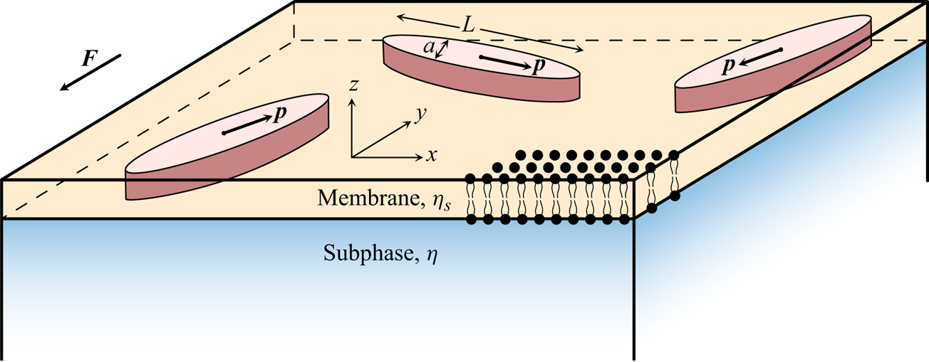
Figure 1. System geometry: elongated particles ( $L\gg a$) are embedded within an infinitesimally thin 2-D viscous layer atop a 3-D fluid subphase, and are all driven in the membrane plane by an external force
  $\boldsymbol {F}$.
2.2. Micromechanical model
We will explore the response of such a quasi-2-D suspension of elongated particles to an externally applied force. For simplicity, the force  $\boldsymbol {F}$ will be taken to be a constant and act in the same direction on all particles, akin to sedimentation in 3-D suspensions (Koch & Shaqfeh Reference Koch and Shaqfeh1989). This might represent tethered trans-membrane proteins that are driven by the external environment or by the cytoskeleton; alternatively, this geometry represents proteins or probes dragged through a membrane or a monolayer by an external force. The translational velocity in (2.3) then has contributions from the self-mobility of each particle, and from advection due to the disturbance field generated by neighbouring rods:
 \begin{equation} \dot{\boldsymbol{x}} = \boldsymbol{u}_{s}+\boldsymbol{u}_{d}. \end{equation}
 Phospholipids that make up biological membranes and monolayers are insoluble and well-approximated as 2-D incompressible fluids (Manikantan & Squires Reference Manikantan and Squires2020). The disturbance field  $\boldsymbol {u}_{d}$ then solves the Boussinesq–Scriven equation (Scriven Reference Scriven1960) for the stress balance within a viscous incompressible interface of surface viscosity
  $\eta _s$ coupled to 3-D Stokes flow in the adjacent bulk fluid of viscosity
  $\eta$ and forced by
  $\boldsymbol {F}$ distributed at concentration
  $c(\boldsymbol {x},t)$:
 \begin{equation} \boldsymbol{\nabla}_{s} \varPi = \eta_s \nabla_{s}^2 \boldsymbol{u}_{d} - \eta \left. \frac{\partial \boldsymbol{v}}{\partial z} \right|_{z=0} + \boldsymbol{F} c(\boldsymbol{x},t),\quad \boldsymbol{\nabla}_{s} \boldsymbol{\cdot} \boldsymbol{u}_{d} = 0. \end{equation}
Here,  $\varPi$ is the surface pressure. Membrane flow is coupled to the 3-D flow field
  $\boldsymbol {v}$ in the adjacent semi-infinite (
 $z$ from
  $0$ to
  $- \infty$) subphase via the traction term and a no-slip condition
  $\boldsymbol {u}=\boldsymbol {v}$ at
  $z=0$. This framework can be generalized to accommodate membrane curvature and to the presence of 3-D fluids on either side of the membrane (Shi et al. Reference Shi, Moradi and Nazockdast2022; Shi, Moradi & Nazockdast Reference Shi, Moradi and Nazockdast2024).
The velocity  $\boldsymbol {u}_{s}$ in (2.5) is the local response of a rod-like particle to a constant force
  $\boldsymbol {F}$:
 \begin{equation} \boldsymbol{u}_{s} = \mu_\perp ({{\boldsymbol{\mathsf{I}}}} - \boldsymbol{p} \boldsymbol{p}) \boldsymbol{\cdot} \boldsymbol{F} + \mu_\parallel \boldsymbol{p}\boldsymbol{p}\boldsymbol{\cdot}\boldsymbol{F}, \end{equation}
with hydrodynamic mobilities  $\mu _\perp$ and
  $\mu _\parallel$ for translation in directions perpendicular and parallel to
  $\boldsymbol {p}$, respectively. These mobilities can be determined by adapting standard boundary integral methods to a slender rod. In short, this is achieved by evaluating the disturbance velocity due to a line distribution of point-force solutions of the Boussinesq–Scriven equation (2.6a,b), and then integrating the force density that satisfies the boundary condition corresponding to particle motion parallel or perpendicular to the force (Fischer Reference Fischer2004; Levine et al. Reference Levine, Liverpool and MacKintosh2004; Shi et al. Reference Shi, Moradi and Nazockdast2022). These integrals can be analytically performed in the asymptotic limits of membrane-dominant (
 $\eta _s\gg \eta L$) or subphase-dominate (
 $\eta _s\ll \eta L$) systems. Specifically, the hydrodynamic mobilities of a rod in a planar incompressible membrane when surface viscous stresses dominate (
 $\eta _s/(\eta L) \rightarrow \infty$) are (Fischer Reference Fischer2004)
 \begin{equation} \mu_\parallel = \frac{\log(8 \eta_s/(\eta L))-\gamma_E+1/2}{4 {\rm \pi}\eta_s},\quad \mu_\perp = \frac{\log(8 \eta_s/(\eta L))-\gamma_E-1/2}{4 {\rm \pi}\eta_s}, \end{equation}
where  $\gamma _E$ is Euler's constant. Notably, drag on a rod-like particle depends only weakly on its length and orientation unlike in 3-D fluids where
  $\mu ^{3D}_\parallel \approx 2 \mu ^{3D}_\perp$. However, the parallel and perpendicular mobilities are not identical (
 $\mu _\parallel -\mu _\perp \rightarrow 1/(4 {\rm \pi}\eta _s)$ as
  $\eta _s/(\eta L) \rightarrow \infty$) and the resulting anisotropy, although weak, affects the suspension microstructure as we see in §§ 3–4. By contrast, the mobilities for subphase-dominant systems (
 $\eta _s/(\eta L) \rightarrow 0$) limit to
 \begin{equation} \mu_\parallel = \frac{\ln(0.48 \eta L / \eta_s)}{{\rm \pi} \eta L},\quad \mu_\perp = \frac{1}{{\rm \pi} \eta L}. \end{equation}
Perpendicular translation in a nearly inviscid membrane represents the most striking difference with 3-D fluids: in-plane 2-D incompressibility displaces surface velocities (and therefore bulk streamlines) around the length of the rod giving rise to a perpendicular drag that is linear in  $L$. Mobility coefficients
  $\mu _\parallel$ and
  $\mu _\perp$ for intermediate values of
  $\eta _s/(\eta L)$ can be evaluated numerically (Fischer Reference Fischer2004; Levine et al. Reference Levine, Liverpool and MacKintosh2004) and they monotonically interpolate between (2.8a,b) and (2.9a,b); further,
  $\mu _\parallel$ is always greater than
  $\mu _\perp$.
Finally, the rotational flux in (2.3) captures reorientation due to non-uniform disturbance fields. For slender rod-like particles, this is given by Jeffery's equation (Jeffery Reference Jeffery1922):
 \begin{equation} \dot{\boldsymbol{p}} = ({{\boldsymbol{\mathsf{I}}}} -\boldsymbol{p}\boldsymbol{p})\boldsymbol{\cdot}\boldsymbol{\nabla}_{s}\boldsymbol{u}_{d} \boldsymbol{\cdot} \boldsymbol{p}. \end{equation}
Thermal noise may contribute additional terms to  $\dot {\boldsymbol {x}}$ and
  $\dot {\boldsymbol {p}}$, or equivalently as diffusive terms in the conservation equation (2.3). We ignore diffusion in what follows to highlight the role of hydrodynamics alone. However, diffusion is straightforward to add to the analysis below via an additional flux
  $-D \boldsymbol {\nabla }_{s} (\ln \psi )$ or equivalently directly as a diffusive term
  $D \nabla _{s}^2 \psi$ on the right-hand side of (2.3), where
  $D$ is a diffusion constant. Diffusion always acts to suppress large wavenumber fluctuations (Manikantan et al. Reference Manikantan, Li, Spagnolie and Saintillan2014; Vig & Manikantan Reference Vig and Manikantan2023).
3. Linear stability
We wish to examine the linear stability of a dilute quasi-2-D suspension that is homogeneous in concentration and isotropic in orientational distribution. The disturbance field associated with such a base state is  $\boldsymbol {u}_{d}=\boldsymbol {0}$. We perturb the probability distribution around this base state as
  $\psi (\boldsymbol {x},\boldsymbol {p},t) = n [ \psi _0 +\epsilon \psi '(\boldsymbol {x},\boldsymbol {p},t) ]$ where
  $\psi _0=(2{\rm \pi} )^{-1}$,
  $\boldsymbol {u}_{d}=\epsilon \boldsymbol {u}'_{d}$ and
  $\dot {\boldsymbol {p}}_{d}=\epsilon \dot {\boldsymbol {p}}'_{d}$. Here,
  $|\epsilon| << 1$ and primes represent perturbed quantities. The corresponding local concentration is
  $c=n [1+\epsilon c' ]$. Plugging perturbed quantities into (2.3) and recognizing the isotropic base state as well as 2-D incompressibility of the membrane fluid field (
 $\boldsymbol {\nabla }_{s}\boldsymbol {\cdot } \boldsymbol {u} = 0$) gives the probability conservation equation at
  $O(\epsilon )$:
 \begin{equation} \frac{\partial{\psi'}}{\partial{t}} + \boldsymbol{\nabla}_{s}\psi'\boldsymbol{\cdot} \boldsymbol{u}_{s} + \psi_0 \boldsymbol{\nabla}_{p}\boldsymbol{\cdot} \dot{\boldsymbol{p}}'_{d} = 0 \end{equation}
We then impose normal modes with wave vector  $\boldsymbol{k}$ and frequency
  $\omega$ of the form
 \begin{equation} \psi'(\boldsymbol{x},\boldsymbol{p},t) = \tilde{\psi}(\boldsymbol{k},\boldsymbol{p},\omega) \exp({{\rm i} (\boldsymbol{k}\boldsymbol{\cdot} \boldsymbol{x} - \omega t)}), \end{equation}
where tildes represent corresponding Fourier variables, so that  $\tilde {c}(\boldsymbol {k},\omega )=\int \tilde {\psi } \,\mathrm {d}\boldsymbol {p}$ is the associated local concentration. The associated hydrodynamic disturbance field can be obtained by solving (2.6a,b) for the corresponding Fourier transform of the disturbance velocity (Manikantan & Squires Reference Manikantan and Squires2020):
 \begin{equation} \tilde{\boldsymbol{u}}_d(\boldsymbol{k},\boldsymbol{p},\omega) = \frac{({{\boldsymbol{\mathsf{I}}}} - \hat{\boldsymbol{k}}\hat{\boldsymbol{k}})\boldsymbol{\cdot} n \boldsymbol{F} \tilde{c}}{k^2 \eta_s+k \eta}, \end{equation}
where  $k=|\boldsymbol {k}|$ and
  $\hat {\boldsymbol {k}}=\boldsymbol {k}/k$ is a unit vector. Then, using Jeffery's equation (2.10), we find
 \begin{align} \tilde{\kern
1.5pt\dot{\boldsymbol{p}}}_{d} = \frac{{\rm i}
(\kern0.7pt \boldsymbol{p}\boldsymbol{\cdot}\boldsymbol{k})
({{\boldsymbol{\mathsf{I}}}} - \boldsymbol{p}\boldsymbol{p})
\boldsymbol{\cdot} ({{\boldsymbol{\mathsf{I}}}} -
\hat{\boldsymbol{k}} \hat{\boldsymbol{k}})
\boldsymbol{\cdot} n \boldsymbol{F} \tilde{c}}{k^2 \eta_s+k
\eta} \Rightarrow \boldsymbol{\nabla}_{p}\boldsymbol{\cdot}
\tilde{\kern 1.5pt\dot{\boldsymbol{p}}}_{d} = \frac{-2{\rm
i} (\kern0.7pt \boldsymbol{p}\boldsymbol{\cdot}\boldsymbol{k})
\boldsymbol{p} \boldsymbol{\cdot} ({{\boldsymbol{\mathsf{I}}}} -
\hat{\boldsymbol{k}} \hat{\boldsymbol{k}})
\boldsymbol{\cdot} n \boldsymbol{F} \tilde{c}}{k^2 \eta_s+k
\eta}. \end{align}
\begin{align} \tilde{\kern
1.5pt\dot{\boldsymbol{p}}}_{d} = \frac{{\rm i}
(\kern0.7pt \boldsymbol{p}\boldsymbol{\cdot}\boldsymbol{k})
({{\boldsymbol{\mathsf{I}}}} - \boldsymbol{p}\boldsymbol{p})
\boldsymbol{\cdot} ({{\boldsymbol{\mathsf{I}}}} -
\hat{\boldsymbol{k}} \hat{\boldsymbol{k}})
\boldsymbol{\cdot} n \boldsymbol{F} \tilde{c}}{k^2 \eta_s+k
\eta} \Rightarrow \boldsymbol{\nabla}_{p}\boldsymbol{\cdot}
\tilde{\kern 1.5pt\dot{\boldsymbol{p}}}_{d} = \frac{-2{\rm
i} (\kern0.7pt \boldsymbol{p}\boldsymbol{\cdot}\boldsymbol{k})
\boldsymbol{p} \boldsymbol{\cdot} ({{\boldsymbol{\mathsf{I}}}} -
\hat{\boldsymbol{k}} \hat{\boldsymbol{k}})
\boldsymbol{\cdot} n \boldsymbol{F} \tilde{c}}{k^2 \eta_s+k
\eta}. \end{align}
Plugging (3.2) and (3.4) into (3.1) gives
 \begin{equation} (-{\rm i} \omega + {\rm i} \boldsymbol{k} \boldsymbol{\cdot} \boldsymbol{u}_{s}) \tilde{\psi} - \frac{2{\rm i} \psi_0 (\kern 1.5pt\boldsymbol{p}\boldsymbol{\cdot}\boldsymbol{k}) \boldsymbol{p} \boldsymbol{\cdot} ({{\boldsymbol{\mathsf{I}}}} - \hat{\boldsymbol{k}} \hat{\boldsymbol{k}}) \boldsymbol{\cdot} n \boldsymbol{F} \tilde{c}}{k^2 \eta_s+k \eta} = 0, \end{equation}
where  $\boldsymbol {u}_{s}$ follows (2.7).
We now non-dimensionalize over characteristic values of  $L$ for length,
  $F$ for force, and
  $F/(4{\rm \pi} \eta _s)$ for velocities. We will take the direction of the force to be
  $\hat {\boldsymbol {f}}$ so that
  $\boldsymbol {F}=F \hat {\boldsymbol {f}}$. Then,
 \begin{equation} (-\omega + \boldsymbol{k} \boldsymbol{\cdot} [\mu_\parallel\boldsymbol{p}\boldsymbol{p} + \mu_\perp ({{\boldsymbol{\mathsf{I}}}} - \boldsymbol{p}\boldsymbol{p})] \boldsymbol{\cdot} \hat{\boldsymbol{f}}) \tilde{\psi} - \frac{8 N\psi_0 \ell (\kern 1.5pt\boldsymbol{p}\boldsymbol{\cdot}\boldsymbol{k}) \boldsymbol{p} \boldsymbol{\cdot} ({{\boldsymbol{\mathsf{I}}}} - \hat{\boldsymbol{k}} \hat{\boldsymbol{k}}) \boldsymbol{\cdot} \hat{\boldsymbol{f}} \tilde{c}}{k^2 \ell+k } = 0, \end{equation}
where  $\ell =\eta _s/(\eta L)$ is the dimensionless Saffman–Delbrück length. Alternatively,
  $\ell$ can be interpreted as a Boussinesq number (Manikantan & Squires Reference Manikantan and Squires2020) which characterizes surface viscous stresses relative to 3-D viscous stresses from the adjacent subphase fluid over the length
  $L$. Momentum transport is membrane-dominated when
  $\ell \rightarrow \infty$ and subphase-dominated when
  $\ell \rightarrow 0$. The variable
  $N=n{\rm \pi} L^2$ is an effective area fraction occupied by particles. The long-ranged description is valid only in the dilute regime, and so
  $N$ is at most
  $O(1)$.
To proceed, we simplify our problem by considering only perturbations in concentration along the direction perpendicular to the external forces:  $\boldsymbol {k} \boldsymbol {\cdot } \hat {\boldsymbol {f}} = 0$. This is motivated by the fact that these transverse perturbations are the most unstable in analogous 3-D sedimentation problems (Koch & Shaqfeh Reference Koch and Shaqfeh1989) and driven 2-D suspensions (Vig & Manikantan Reference Vig and Manikantan2023). Simplifying with this assumption and rearranging gives
 \begin{equation} \tilde{\psi} = \left(\frac{8 N\psi_0 \ell \tilde{c}}{k^2 \ell+k }\right) \frac{(\kern 1.5pt\boldsymbol{p}\boldsymbol{\cdot}\boldsymbol{k}) (\kern 1.5pt\boldsymbol{p}\boldsymbol{\cdot}\hat{\boldsymbol{f}}) }{(\mu_\parallel - \mu_\perp)(\kern 1.5pt\boldsymbol{p}\boldsymbol{\cdot}\boldsymbol{k}) (\kern 1.5pt\boldsymbol{p}\boldsymbol{\cdot}\hat{\boldsymbol{f}}) -\omega} . \end{equation}
Integrating (3.7) across all orientations while noting that  $\tilde {c}(\boldsymbol {k},\omega )=\int \tilde {\psi } \,\mathrm {d}\boldsymbol {p}$ eliminates
  $\tilde {\psi }$ to reveal an implicit relationship for
  $\omega (k)$:
 \begin{equation} \int \frac{(\kern 1.5pt\boldsymbol{p}\boldsymbol{\cdot}\boldsymbol{k}) (\kern 1.5pt\boldsymbol{p}\boldsymbol{\cdot}\hat{\boldsymbol{f}}) }{(\mu_\parallel - \mu_\perp)(\kern 1.5pt\boldsymbol{p}\boldsymbol{\cdot}\boldsymbol{k}) (\kern 1.5pt\boldsymbol{p}\boldsymbol{\cdot}\hat{\boldsymbol{f}}) -\omega} \mathrm{d} \boldsymbol{p} = \frac{k^2 \ell+k }{8 N \psi_0 \ell }. \end{equation}
The mobility coefficients  $\mu _\parallel$ and
  $\mu _\perp$ are functions of
  $\ell$, and
  $\psi _0=(2{\rm \pi} )^{-1}$ is the isotropic base state distribution. For a given area fraction
  $N$, (3.8) thus represents a family of dispersion relations parametrized by the Saffman–Delbrück length
  $\ell$.
In a 2-D Cartesian plane representing the membrane, we can take  $\hat {\boldsymbol {f}}=-\hat {\boldsymbol {y}}$ and
  $\hat {\boldsymbol {k}}=\hat {\boldsymbol {x}}$ without loss of generality. Simplifying (3.8) using
  $\boldsymbol {p}=(\cos \theta,\sin \theta )$ then gives
 \begin{equation} \frac{1}{2{\rm \pi}}\int_0^{2{\rm \pi}} \frac{k \sin \theta \cos \theta }{(\mu_\parallel - \mu_\perp)k \sin \theta \cos \theta +\omega} \mathrm{d} \theta = \frac{k^2 \ell+k }{8 N \ell }, \end{equation}
which is an implicit integral equation for the dispersion relation  $k(\omega )$. For normal modes of the form
  $\exp [{\rm i} (\boldsymbol {k}\boldsymbol {\cdot } \boldsymbol {x} - \omega t)]$, perturbations are unstable if the imaginary part of
  $\omega$ is positive.
Figure 2(a) shows the growth rate  $\sigma =\mbox {Im}[\omega ]$ as a function of wavenumber obtained by numerically evaluating roots of (3.9) with a secant method. The
  $\ell \rightarrow \infty$ limit is reminiscent of analogous 3-D suspensions, where the system-spanning mode corresponding to
  $k=0$ is the most unstable (see Koch & Shaqfeh Reference Koch and Shaqfeh1989; Manikantan et al. Reference Manikantan, Li, Spagnolie and Saintillan2014). To obtain the growth rate at
  $k=0$ analytically, we expand the integrand in (3.9) as a Taylor series in
  $k$:
$k$:
 \begin{equation} \frac{k}{2{\rm \pi} \omega}\int_0^{2{\rm \pi}} \sin\theta\cos\theta \left[1- \frac{(\mu_\parallel - \mu_\perp)k}{\omega} \sin\theta\cos\theta + \cdots \right] \mathrm{d} \theta =\frac{k^2 \ell+k }{8 N \ell }. \end{equation}
Integrating term by term and simplifying gives
 \begin{equation} {-}\frac{(\mu_\parallel - \mu_\perp) k^2}{\omega^2} + O(k^4)= \frac{k^2 \ell + k}{N\ell}. \end{equation}
From (2.8a,b), the dimensionless mobility difference in the membrane-dominated regime ( $\ell \rightarrow \infty$) is
  $\mu _\parallel - \mu _\perp \rightarrow 1$, which gives
  $\omega ^2=-N+O(k^2)$ or
 \begin{equation} \sigma (k\rightarrow 0, \ell\rightarrow \infty) = \sqrt{N}. \end{equation}
In fact, this turns out to be the maximum value of the growth rate across all  $k$ and
  $\ell$.

Figure 2. (a) Growth rates  $\sigma$ of unstable modes at various
  $\ell =\eta _s/\eta L$ for a dimensionless number density of
  $N=n {\rm \pi}L^2=1$. (b) Maximum growth rate
  $\sigma _m$, and (c) most unstable wavenumber
  $k_m$ and largest wavenumber
  $k_0$ as a function of
  $\ell$. Dashed lines in (c) are asymptotic limits from (3.14a,b).
Increasing subphase viscous stresses (decreasing  $\ell$) always acts to suppress the instability. Notably, the
  $k=0$ mode is stable for finite
  $\eta$, reflecting a boundary layer at infinity that regularizes the singularity in 2-D Stokes by accounting for subphase viscous stresses (Saffman Reference Saffman1976). For finite
  $\ell$, (3.11) gives
  $\omega ^2 \sim - k N \ell (\mu _\parallel - \mu _\perp )$ or
  $\sigma =\mbox {Im}[\omega ] \propto \sqrt {k}$. In other words, the growth rate goes to zero as
  $k\rightarrow 0$ for all values of
  $\ell$ except in the limit
  $\ell \rightarrow \infty$. The most unstable mode then corresponds to a finite value of
  $k$ which suggests a mechanism for wavenumber selection. The most unstable wavenumber
  $k_m$ can be determined by taking the derivative of (3.9) with respect to
  $k$ and numerically solving the implicit integral equation corresponding to
  $\partial \omega /\partial k = 0$. Figure 2(b,c) shows
  $k_m$ and the corresponding growth rate
  $\sigma _m$ as a function of
  $\ell$. Note that the maximum growth rate
  $\sigma _m$ asymptotes to the
  $\ell \rightarrow \infty$ limit as predicted by (3.12), and monotonically decreases upon decreasing
  $\ell$. The wavenumber
  $k_m$ corresponding to fastest growth of perturbations, however, varies non-monotonically with
  $\ell$ and peaks at
  $\ell =O(1)$: in § 4 we propose a mechanism of instability that clarifies the length scale selection underlying
  $k_m$ and its dependence on
  $\ell$.
Finally, a key parameter is the largest unstable wavenumber  $k_0$ which reveals the length scale of shortest unstable modes. Setting
  $\omega =0$ in (3.9) gives
 \begin{equation} k_0^2 \ell+k_0=\frac{8 N \ell}{\mu_\parallel - \mu_\perp}. \end{equation}
Solving this quadratic equation for positive  $k_0$ yields the curve in figure 2(c). Note that this
  $\omega =0$ limit is only valid for
  $k\neq 0$. The range of unstable modes increases monotonically with
  $\ell$. The high and low
  $\ell$ limits can be found analytically using (2.8a,b) and (2.9a,b):
  $\mu _\parallel - \mu _\perp$ asymptotes to
  $1$ and
  $4\ell [ \ln (0.48/ \ell )-1 ]$ in these limits, respectively, giving
 \begin{equation} k_0 (\ell \rightarrow \infty) = \sqrt{8N},\quad k_0 (\ell \rightarrow 0)= \frac{2N}{-\log(\ell)-1.73}. \end{equation}
These are shown as the dashed curves in figure 2(c).
4. Instability mechanism and length-scale selection
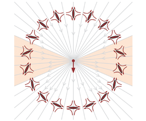
The mechanism of instability can be understood by examining the disturbance flow created in the plane of the membrane by a point force and the effect of this flow on realigning neighbouring particles. We again follow classic 3-D suspension works (Koch & Shaqfeh Reference Koch and Shaqfeh1989) to examine relative alignment of pairs of particles under a pseudo-steady approximation where particle positions are held at a fixed distance. In a dilute suspension, any given particle creates a point-force velocity disturbance (shown as the arrow pointing downward in figure 3a,b). Neighbouring particles tend to align parallel to the direction of the extensional component (shown in magenta around each particle) of the fluid motion caused by the point force at the centre. Such a picture helps identify microstructural configurations that favour accumulation or separation.

Figure 3. Mechanism of the instability: a point force generates in-plane velocity  $\boldsymbol {u}$ (grey streamlines). The magenta streamlines depict the symmetric part of the local, linear flow field around particles at a distance
  $r$. Particles are shown in their most favoured orientation, with their long axis parallel to the extensional component of the flow field generated by the point force. (a) For
  $\ell \gg r$ (membrane-dominated regime), neighbours always reorient such that they are drawn towards the point force, thereby increasing particle density. (b) By contrast, at much longer length scales
  $r \gg \ell$ (subphase-dominated regime), particles that fall within the shaded region reorient such that they are drawn away from the point force, reducing particle density and stabilizing the suspension. For a fixed
  $\eta _s$ and
  $\eta$, the system transitions continuously from membrane-dominated to subphase-dominated at large enough distances.
We can evaluate the local extensional flow and the principal axes of extension around each particle from the hydrodynamic disturbance field due to the point force. The dimensionless velocity at a point  $\boldsymbol {r}$ in the plane of the membrane due to a point force at the origin is (Fischer Reference Fischer2004; Levine et al. Reference Levine, Liverpool and MacKintosh2004; Manikantan & Squires Reference Manikantan and Squires2020)
 \begin{align} \boldsymbol{u} (\boldsymbol{r}) &= {\rm \pi}\left[ \left( \frac{H_1(d)}{d} -\frac{2}{{\rm \pi} d^2} - \frac{Y_0(d)+Y_2(d)}{2} \right) \frac{\boldsymbol{r} \boldsymbol{r}}{r^2} \right. \nonumber\\ &\quad + \left. \left(H_0(d)- \frac{H_1(d)}{d} +\frac{2}{{\rm \pi} d^2} - \frac{Y_0(d)-Y_2(d)}{2} \right) \left( {{\boldsymbol{\mathsf{I}}}} - \frac{\boldsymbol{r} \boldsymbol{r}}{r^2} \right) \right]\boldsymbol{\cdot} \hat{\boldsymbol{f}}, \end{align}
where  $r=|\boldsymbol {r}|$ is the dimensionless distance, and
  $d=r/\ell$. Here,
  $H_\nu$ and
  $Y_\nu$ are Struve and Bessel functions of the second kind or order
  $\nu$, respectively. Note that
  $\ell$ is renormalized by the distance
  $r$ in the far-field description: in other words, at constant
  $\eta _s$ and
  $\eta$, the system switches from membrane-dominated to subphase-dominated at large enough length scales.
The velocity field in the plane of the membrane from (4.1) asymptotes to that corresponding to the 2-D stokeslet in the membrane-dominated regime ( $\ell \gg r$):
 \begin{equation} \boldsymbol{u} (\boldsymbol{r},\ell\gg r) \rightarrow \left[ -\log\left( \frac{r}{\ell}\right){{\boldsymbol{\mathsf{I}}}} + \frac{\boldsymbol{r} \boldsymbol{r}}{r^2} \right] \boldsymbol{\cdot} \hat{\boldsymbol{f}}. \end{equation}
The mechanism of the instability is tied to the reorientation of neighbouring particles when placed in such a disturbance field. Specifically, rod-like particles align with the extensional axis of the local flow. The rate-of-strain tensor in the membrane-dominated case is
 \begin{equation} {{\boldsymbol{\mathsf{E}}}} (\ell \gg r ) = \frac{\boldsymbol{\nabla}_{s} \boldsymbol{u}_{d} + \boldsymbol{\nabla}_{s} \boldsymbol{u}_{d}^T}{2} = \frac{(\boldsymbol{r} \boldsymbol{\cdot} \hat{\boldsymbol{f}}) {{\boldsymbol{\mathsf{I}}}} }{r^2} - \frac{ 2 \boldsymbol{r} \boldsymbol{r} \boldsymbol{r} \boldsymbol{\cdot} \hat{\boldsymbol{f}}}{r^4}. \end{equation}
Using  $\hat {\boldsymbol {f}}=-\hat {\boldsymbol {y}}$ and
  $\boldsymbol {r}=r \hat {\boldsymbol {r}} = (r \cos \phi, r\sin \phi )$ where
  $\phi$ is measured relative to the positive
  $x$ direction diagonalizes the rate-of-strain tensor in the
  $(\hat {\boldsymbol {r}},\hat {\boldsymbol {\phi }})$ basis as
 \begin{equation} {{\boldsymbol{\mathsf{E}}}} (\ell\gg r ) = \frac{\sin \phi}{r} \begin{bmatrix} 1 & 0 \\ 0 & -1 \end{bmatrix} . \end{equation}
The eigenvectors of  ${{\boldsymbol{\mathsf{E}}}}$ are the principal directions of extension. We see from (4.4) that the principal axis of extension is parallel to
  $\hat {\boldsymbol {r}}$ – i.e. along the line connecting the particle to the point force – in the upper half-plane (
 $\phi >0$) and perpendicular to
  $\hat {\boldsymbol {r}}$ in the lower half (
 $\phi <0$). Figure 3(a) shows particles in such a preferred alignment: the anisotropic mobility of each elongated particle then draws it towards the point force, leading to a net tendency for particles to accumulate and amplify concentration fluctuations. This is analogous to the classic 3-D instability in the suspension of a rod (see Koch & Shaqfeh Reference Koch and Shaqfeh1989). Note also from (4.4) that the eigenvalues of
  ${{\boldsymbol{\mathsf{E}}}}(\ell \gg r)$, corresponding to the local rates of extension
  $\lambda _{ext}$, peak at
  $\phi =\pm \frac {1}{2}{\rm \pi}$ and vanish at
  $\phi =0$: rods on the same horizontal line thus do not reorient in response to the disturbance due to the other.
The in-plane extensional field surrounding a point force changes dramatically upon increasing the contribution from the subphase (decreasing  $\ell$). The membrane velocity field in the surface-inviscid limit (
 $\ell \ll r$) is
 \begin{equation} \boldsymbol{u} (\boldsymbol{r},\ell \ll r ) \rightarrow 2 \ell \frac{\boldsymbol{r} \boldsymbol{r}}{r^3} \boldsymbol{\cdot} \hat{\boldsymbol{f}}. \end{equation}
Note that (4.5) is not simply a 2-D slice of the flow due to a point force in the bulk 3-D fluid: surface incompressibility requires that  $\boldsymbol {u}$ be divergence-free in the plane of the membrane. The rate-of-strain tensor is no longer easily diagonalizable in the
  $(\hat {\boldsymbol {r}},\hat {\boldsymbol {\phi }})$ basis; however,
  ${{\boldsymbol{\mathsf{E}}}}$ still reveals key features when expressed in the
  $(\hat {\boldsymbol {x}},\hat {\boldsymbol {y}})$ basis:
 \begin{equation} {{\boldsymbol{\mathsf{E}}}} (\ell \ll r ) = \frac{2 \ell}{r^2} \begin{bmatrix} \sin \phi (3 \cos^2 \phi -1) & \cos\phi\left(3 \sin^2\phi-\frac{1}{2}\right) \\ \cos\phi\left(3 \sin^2\phi-\frac{1}{2}\right) & \sin\phi(3\sin^2\phi-2) \end{bmatrix} . \end{equation}
First, principal rates of extension scale with  $\ell$, consistent with a weakening instability as seen in § 3. Additionally, neighbouring particles along the wave vector (on the same horizontal line as the point force, or along
  $\phi =0$) experience a non-zero rate of extension along a principal direction
  $\theta _{ext}=3{\rm \pi} /4$ (figure 4). Coupled to the anisotropic mobility of rods, local extension therefore reorients rods in a manner that draws them away from the reference particle if initially placed in a region near
  $\phi =0$, which acts as a stabilizing mechanism. Note also from (4.6) that
  ${{\boldsymbol{\mathsf{E}}}}$ is diagonal in the
  $(\hat {\boldsymbol {x}},\hat {\boldsymbol {y}})$ basis when
  $3 \sin ^2\phi =\frac {1}{2}$, i.e. for a critical angle
  $\phi _c=\pm \sin ^{-1}(1/\sqrt {6})$. This corresponds to principal axes that are aligned with
  $\hat {\boldsymbol {x}}$ or
  $\hat {\boldsymbol {y}}$ and reveals a transition from configurations that draw neighbouring particles towards the point force (when
  $|\phi |>|\phi _c|$) or away from it. This also suggests a mechanism for wavenumber selection as seen in the stability analysis in § 3: the critical length scale emerges from a balance of fluxes of particles driven out from within the region
  $|\phi |<|\phi _c|$ vs drawn in from regions where
  $|\phi |>|\phi _c|$.

Figure 4. (a) Principal axes of stretch  $\theta _{ext}$ corresponding to preferred orientation of a neighbouring particle as a function of azimuthal position
  $\phi$ around a reference particle for
  $\ell /r=0.1$ (dotted line),
  $1$ (dash-dot) and
  $10$ (dashed line). The shaded patch denotes the set of orientations that draws particles away from each other: this region is not accessed in the limit of
  $\ell \rightarrow \infty$ (solid line), whereas
  $\ell \rightarrow 0$ maximizes this window for a range of relative positions
  $|\phi |<|\phi _c|=\sin ^{-1}(1/\sqrt {6})$. (b) Principal rates of extension
  $\lambda _{ext}$ corresponding to cases shown in (b). (c) The principal rate
  $\lambda _{ext}$ does not vanish at
  $\phi =0$ for finite
  $\ell$, and peaks when
  $r\sim \ell$.
Principal directions of extension for arbitrary  $\ell$, obtained by numerically evaluating the eigenvectors of
  ${{\boldsymbol{\mathsf{E}}}}$ from the general velocity field in (4.1), are shown in figure 4(a). This further clarifies the emergence of a ‘stabilizing region’ in terms of preferred orientations for finite
  $\ell$. Particles placed in this region are drawn away from the reference particle, contributing to a suppression of the instability. The
  $\ell /r \rightarrow \infty$ limit avoids this region entirely as seen mechanistically in figure 3 and quantitatively as a discontinuity in
  $\theta _{ext}(\phi )$ in figure 4(a). This reflects the singularity of 2-D Stokes flow at infinity, and the subphase viscous contribution introduces a boundary layer that regularizes this discontinuity. In doing so,
  $\theta _{ext}$ takes on values that fall within the shaded patch in figure 4(a) that represents a stabilizing region, where particle orientations are such that they are drawn away from the reference particle. This mechanism also explains the stabilization of the
  $k=0$ mode for finite
  $\ell$ in § 3: for any
  $\eta$ and
  $\eta _s$ (and since
  $\boldsymbol {k}$ is parallel to
  $\hat {\boldsymbol {x}}$ for transverse perturbations), particles along the horizontal line (
 $\phi =0$) will always fall in the stabilizing region at a large enough value of
  $r$.
$r$.
The associated eigenvalues of  ${{\boldsymbol{\mathsf{E}}}}$ are local rates of extension
  $\lambda _{ext}$: while these principal rates always peak at
  $\phi =\pm \frac {1}{2}{\rm \pi}$ and their magnitudes decrease upon decreasing
  $\ell$, they do not always vanish at
  $\phi =0$ (figure 4b,c). Indeed,
  $\lambda _{ext}(r,\phi =0)$ peaks when
  $r\sim \ell$. For a pair of particles placed in the same horizontal line, the reorientation that favours particle separation is thus strongest at distances comparable to the Saffman–Delbrück length.
5. Conclusion
In this paper, we developed a mean-field model to examine hydrodynamic collective modes of elongated particles embedded in viscous membranes or monolayers. We focused on a linear stability analysis around a homogeneous and isotropic quasi-2-D suspension of such particles. We discover a unique mechanism for stabilization of such a system, reflecting aspects of the Stokes paradox in 2-D viscous flows and its regularization via 3-D subphase stresses. We then tie this mechanism to the interplay between anisotropic particle mobility and long-ranged hydrodynamics in the plane of the membrane.
More generally, this mean-field framework opens a rich avenue of fluid dynamical problems and tools to examine microstructure on biological or synthetic membranes. The method can be readily adapted to membranes with curvature using modified Green's functions (Shi et al. Reference Shi, Moradi and Nazockdast2022, Reference Shi, Moradi and Nazockdast2024), to active particles on membranes via a stresslet solution (Oppenheimer et al. Reference Oppenheimer, Stein and Shelley2019; Manikantan Reference Manikantan2020), and to systems with weakly non-Newtonian membrane rheology using tools such as the Lorentz reciprocal theorem (Vig & Manikantan Reference Vig and Manikantan2023). We have illustrated the ‘deep’ subphase limit: confining the 3-D fluid has been shown to amplify bulk stresses (Camley & Brown Reference Camley and Brown2013; Shi et al. Reference Shi, Moradi and Nazockdast2024) and modify membrane flow fields in manners that favour aggregation (Manikantan Reference Manikantan2020). This modification is also straightforward within the mean-field description developed here. Our findings also open up opportunities to examine nonlinear dynamics in these systems by computationally solving the mean-field model and through efficient particle simulations of crowded systems. Building on these insights, we anticipate that the present work will spur new directions of fluid dynamical studies into active and passive quasi-2-D suspensions.
Funding
This material is based upon work supported by the U.S. National Science Foundation under grant no. CBET-2340415.
Declaration of interests
The author reports no conflict of interest.


 Open access