


1. Introduction
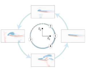
In an increasing number of flight applications, aerodynamic bodies are subject to large, unsteady disturbances, often resulting in separated, vortex-dominated flows (Jones, Cetiner & Smith Reference Jones, Cetiner and Smith2021). These flows are difficult to model in a low-order manner, but conceptually, vortex shedding events are often described in intuitive terms. Consider the problem of a wing encountering a discrete gust, illustrated in figure 1. This flow evolves in roughly three stages: (1) the wing begins in a base state of cruise, likely characterized by attached flow; (2) the wing encounters the gust, which triggers vortex shedding from the leading edge; (3) the wing exits the gust and returns toward its base state. This flow is not periodic and the underlying physics is inherently nonlinear, but in broad terms, these stages of vortex shedding belong to a single cycle, from the base state to a disturbed state and back to the base state.

Figure 1. The broad stages of vortex shedding associated with a transverse gust encounter.
The current work poses the following question: is there a way to describe large-amplitude disturbances that appeals to our intuitive notion of cycles and loops? Historically, cyclic events in aerodynamic flows have been described using Fourier analysis, but for discrete transient manoeuvres, in which the dynamics of the flow is unlikely to conform to a time-periodic basis, it can be difficult to characterize the flow without resorting to a large number of modes. As an alternative, we propose a data-driven framework that characterizes nonlinearly disturbed flows based on their topology, or their shape and structure, in a high-dimensional state space. Our central idea is that large-scale vortex shedding events, while complex and nonlinear in physical space, exhibit a fairly simple topology in state space, which we can leverage to identify low-order, interpretable representations of the flow.
To demonstrate this approach, we consider a set of experimental flowfield measurements in which a flat-plate wing translates horizontally into a transverse gust. For each gust encounter, we analyse the flow in two stages. First, we describe the dynamics of each gust encounter using persistent homology, a method of topology characterization that identifies the generating cycles, or ‘holes’, associated with a point cloud (Edelsbrunner & Morozov Reference Edelsbrunner and Morozov2014). Traditionally, persistent homology has found success in geometry-focused applications, such as medical imaging (Qaiser et al. Reference Qaiser, Sirinukunwattana, Nakane, Tsang, Epstein and Rajpoot2016) and molecular structure identification (Townsend et al. Reference Townsend, Micucci, Hymel, Maroulas and Vogiatzis2020). More recent studies have applied persistent homology to the characterization of dynamical events (Myers, Munch & Khasawneh Reference Myers, Munch and Khasawneh2019), but only a small fraction of these studies consider fluid systems (Kramar et al. Reference Kramar, Levanger, Tithof, Suri, Xu, Paul, Schatz and Mischaikow2016; Liu et al. Reference Liu, Siala, Budišić and Green2020; Wu, Tao & Zheng Reference Wu, Tao and Zheng2021).
Second, we use an autoencoder to transform the full-state dynamics of each gust encounter to a reduced-order space. The autoencoder is a data-driven method of feature extraction, capable of reducing complex fluid flows to a small number of essential state variables (Murata, Fukami & Fukagata Reference Murata, Fukami and Fukagata2020; Fukami & Taira Reference Fukami and Taira2023). In its basic configuration, the autoencoder is constructed as an approximation of an invertible, nonlinear transformation between a high-dimensional space and a low-dimensional space. In this work, we construct an autoencoder such that it transforms the dynamics of each gust encounter to a reduced-order space, while also preserving the most prominent topological features of the system. Our goal is to arrive at a low-order space in which the trajectory of the flow is simple and interpretable, all without sacrificing the reconstruction capabilities of the autoencoder.
In the sections that follow, we present a brief treatise on both persistent homology and nonlinear autoencoders, and we describe how these concepts can be combined to construct topology-preserving maps. We then apply our approach to an experimental gust encounter as a way of demonstrating the utility of this method in compressing, characterizing and modelling large-scale aerodynamic disturbances.
2. Methods
2.1. Persistent homology
In this subsection, we review persistent homology and its application to dynamical systems. Persistent homology is a computational tool for identifying homology groups, or  $k$-dimensional holes, in a multivariate point cloud (Edelsbrunner & Morozov Reference Edelsbrunner and Morozov2014). It characterizes a point cloud based on its topology, or the connectedness of nearby points, and in doing so, provides an avenue for describing the underlying ‘shape’ from which the points are sampled.
Persistent homology is defined formally in the language of simplicial topology, and its mathematical origins have been documented extensively throughout the literature (see Rieck (Reference Rieck2017) for a rigorous but approachable review). We aim to work with a more intuitive understanding of persistent homology, which is best illustrated with an example. Consider a point cloud sampled from a smooth circle embedded in  $\mathbb {R}^2$, sketched in figure 2(a). Let us associate an
  $\epsilon$-sphere with each point in figure 2(a), and examine the intersections that result from gradually increasing its diameter. In particular, we note that there is a certain diameter at which each
  $\epsilon$-sphere intersects with its neighbours, and a ‘hole’ emerges at the centre of the point cloud. Likewise, there is a certain diameter at which all
  $\epsilon$-spheres share a common intersection, and the hole is closed. The persistence (
 $p$) of this hole is defined as the difference between the diameter at which the hole emerges (‘birth’) and the diameter at which the hole is closed (‘death’).

Figure 2. The filtration process for a point cloud sampled (a) from a perfect circle in  $\mathbb {R}^2$, and (b) from the trajectory of a dynamical system.
The procedure above is called a Vietoris–Rips filtration, and it can be used to quantify various topological features in multivariate point cloud data. These features are generally classified according to their homology group  $H_k$ (where
  $k$ is the dimension of the manifold that bounds the feature of interest). Each of these groups can be linked to an intuitive notion of discrete shape or structure. In this work, we focus on two homology groups:
  $H_0$ (which corresponds to connected components) and
  $H_1$ (which corresponds to holes, or 1-cycles). The term ‘connected component’ refers to a collection of points that are linked together through mutual intersection. That is, two data points belong to the same connected component if one can travel between the two points without leaving an
  $\epsilon$-sphere (Zomorodian Reference Zomorodian2005). The notion of a ‘hole’ is exactly what was described in our initial example. That is, we define a hole as a closed loop of
  $\epsilon$-spheres, the collection of which bounds a non-empty surface in ambient space. As an illustration, we note that the leftmost filtration in figure 2(a) exhibits eight connected components and zero holes, while the centre filtration in figure 2(a) exhibits one connected component and one hole.
As a data analysis tool, persistent homology is concerned with how these connected components and holes change over successive values of  $\epsilon$. Such behaviour is typically presented in a persistence diagram, an example of which is provided in figure 2(a) for the circular point cloud. In this figure, the values of
  $\epsilon$ corresponding to the birth of topological features are plotted on the abscissa, while the values of
  $\epsilon$ corresponding to the death of topological features are plotted on the ordinate. Collectively, these birth–death pairs provide a concise description of our point cloud in ambient space, and provide a framework for describing the underlying shape from which our points were sampled.
Let us examine how the birth–death pairs of figure 2(a) relate to the filtration of the circular point cloud. In this example, our dataset consists of eight points, each separated by a distance 0.765 in  $\mathbb {R}^2$. At a low value of
  $\epsilon$, each of these points is immersed in a separate sphere, and our topological space consists of eight separate connected components. At
  $\epsilon =0.765$, each
  $\epsilon$-sphere intersects with its neighbours, and the number of connected components is reduced from eight to one. In turn, the
  $H_0$ group is characterized by seven identical birth–death pairs at
  $(0,0.765)$. Each of these birth–death coordinates corresponds to the intersection of two adjacent connected components; that is, an intersection between two connected components always leads to one ‘death’. Note that the diagram in figure 2(a) also features a final birth–death pair at
  $(0,\infty )$. This point is included as convention and captures the idea that the combined set of intersecting spheres persists as a connected subset to arbitrarily large values of
  $\epsilon$. It also ensures that the total number of
  $H_0$ birth–death pairs is equal to the number of input points.
The  $H_1$ group in figure 2(a) can be interpreted in a similar fashion. At
  $\epsilon =0.765$, the intersections of adjacent
  $\epsilon$-spheres form a closed 1-cycle, and the combined set of spheres exhibits a ‘hole’ at the centre of
  $\mathbb {R}^2$. This ‘hole’ persists for increasing values of
  $\epsilon$ up to
  $\epsilon \approx 2$, at which point any two spheres in the set share a non-zero intersection, and the hole is closed. The
  $H_1$ group is then characterized by a single birth–death pair near
  $(0.765, 2)$, and we observe that the point cloud is characterized by a single large hole. Note that for the
  $H_1$ element in figure 2(a), the ‘death’ coordinate is not exactly
  $\epsilon = 2$ (i.e. the diameter of the circle), but rather
  $\epsilon \approx \sqrt {3}$. This is a consequence of the mathematical definition of a Vietoris–Rips complex; we refer the reader to Zomorodian (Reference Zomorodian2005) and Adamaszek & Adams (Reference Adamaszek and Adams2017) for a detailed, group-theoretic definition of the
  $H_1$ ‘death’ coordinate, and how this definition manifests in the computation of a persistence diagram. For the purposes of this work, we can still rely on the diagram of figure 2(a) for an intuitive idea of when a hole is closed, even if the numerical value on the persistent diagram does not align exactly with our intuition. Also note that the dashed line in figure 2(a) represents minimal persistence (i.e. topological features that emerge and close at the same radius). Later, we will see that this minimum persistence line provides a simple way to distinguish between major topological features and noise in a persistence diagram.
The preceding example of a circular point cloud is simplistic, but the utility of persistent homology lies in the notion that this simple procedure can be applied to point clouds of arbitrary complexity and dimension. As a more practical example, figure 2(b) plots a series of points sampled from a complex curve in  $\mathbb {R}^3$. This curve could be interpreted as the trajectory of a dynamical system, where each axis corresponds to one of three state variables, and each point corresponds to a different instance in time. The rightmost image of figure 2(b) shows the persistence diagram for this point cloud. We see that much like the circular point cloud, this curve is characterized by one highly persistent hole in
  $H_1$. The persistence of the hole in figure 2(b) is quite different from the persistence of the hole in figure 2(a), but from a top level, the two curves share a similar topological description, in that the rank of their
  $H_1$ group is identical. This similarity points towards a more powerful idea: the underlying curve in figure 2(a) is homeomorphic to the unit circle, meaning that there exists an invertible map between the two curves.
In the sections that follow, we apply a similar analysis to the dynamics of an unsteady gust encounter. Our core idea is that if we can identify a simple shape that is topologically similar to the full-state dynamics of a gust encounter, then we can construct a map between the two shapes. Because of turbulence and measurement noise, the full-state dynamics of a gust encounter is unlikely to be exactly homeomorphic to such a simple shape (Wu et al. Reference Wu, Tao and Zheng2021). We aim instead to find a transformation that results in a minimal loss of information, or an ‘approximate’ homeomorphism. We propose that this transformation can be found using a modified autoencoder.
2.2. Autoencoder
In this subsection, we describe a process for finding transformations between high-dimensional trajectories and simple, low-order shapes, a task that we accomplish using an autoencoder. We begin by reviewing the basic framework of the autoencoder, before highlighting how this framework can be augmented through topological data analysis. As a starting point, figure 3 provides a conceptual diagram of our network architecture. In this figure, a time series of flowfield snapshots is mapped from a high-dimensional state space to a low-order (or latent) space by an encoder  $f$, and reverse transformed by a decoder
  $g$. The latent vector
  $\boldsymbol {\xi }$ serves as the bottleneck of the network architecture; its number of components defines the autoencoder compression ratio, and generally corresponds to the minimum number of variables needed to reconstruct the flow. In our implementation, the encoder and decoder are each composed of a convolutional neural network (CNN; Lecun et al. Reference Lecun, Bottou, Bengio and Haffner1998) and a multi-layer perceptron (MLP; Rumelhart & McClelland Reference Rumelhart and McClelland1986). Within these networks, each layer is associated with a set of model weights, and is coupled to adjacent layers by an activation function, for which we choose the hyperbolic tangent. In a process called ‘training’, the value of each weight is determined by minimizing a loss function, which is based conventionally on the difference between the input flowfield and the reconstructed flowfield.

Figure 3. The topological autoencoder used in the present study.
The key feature of our approach is that in addition to constraining the autoencoder to reconstruct the flow, we place topological constraints on the loss function, such that the latent space preserves the most persistent features of the input trajectory (Moor et al. Reference Moor, Horn, Rieck and Borgwardt2020). Figure 3 includes a rough sketch of how we incorporate topological constrains into the training of our autoencoder. For a given time series of flowfields, we compute the persistent homology of the trajectory, and identify the number of elements associated with each homology group  $H_k$. We then manually select a target shape, or a simple analytic curve in
  $\mathbb {R}^2$ or
  $\mathbb {R}^3$, that exhibits the same number of highly persistent holes, or the same rank of each
  $H_k$, as the input trajectory. The effect of persistent homology is then enforced implicitly via the loss function: a new term is added to the loss function that quantifies the difference between the latent trajectory and the target shape. The central idea is that we are forcing the latent trajectory to conform to a simple, tractable shape, and because that shape preserves the topology of the full-state dynamics (i.e. the encoder approximates a homeomorphism), the reconstruction capabilities of the autoencoder should be unaffected.
With the overall goal of our method in mind, we write an expression for the loss function of our autoencoder as
 \begin{equation} \mathcal{L} = \beta_r \left \| \boldsymbol{q} - f \circ g (\boldsymbol{q}) \right \|_2 + \beta_s \left \|\,f(\boldsymbol{q}) - \boldsymbol{s}(\kappa) \right \|_2 + \beta_p \left \langle \,p \left(\,f(\boldsymbol{q}) \right) - p \left(\boldsymbol{s}(\kappa) \right) \right \rangle\!{,} \end{equation}
where  $\boldsymbol {q}$ represents the full state of the flow,
  $\boldsymbol {s}$ represents the trajectory of the target shape (the selection of which depends upon a set of case-dependent parameters
  $\boldsymbol {\kappa }$), and
  $p(\,f(\boldsymbol {q}))$ and
  $p(\boldsymbol {s})$ represent the persistence of the latent trajectory and target shape, respectively. Note that double modulus rules in (2.1) indicate an average among snapshots, while angle brackets indicate an average among trajectories.
Each term in (2.1) serves a specific purpose in ensuring that the autoencoder converges towards a topology-preserving map. The first term in (2.1), called the reconstruction term, ensures that the transformation  $f$ is as close as possible to a bijection. Topologically, it ensures that adjacent vertices in
  $\mathbb {R}^n$ remain adjacent in the latent space. The second term forces the latent trajectory of the system to conform to the target shape (
 $\boldsymbol {s}$). Note that this term assumes that
  $\boldsymbol {s}$ is given analytically, such that
  $f(\boldsymbol {q}) - \boldsymbol {s}(\kappa )$ is the distance between a point and a curve, but it does not assign a specific location along the shape to each encoded snapshot. The final term in (2.1) places a minimum threshold on the persistence of holes (or elements of the
  $H_1$ group) in the latent trajectory. This term is related implicitly to the shape conformation term, in that the persistence threshold is dependent upon target shape selection, but we must note that this term is included in the loss function strictly as an aid to convergence. Setting
  $\beta _p \neq 0$ prevents the autoencoder from finding erroneous local minima (e.g. a jump discontinuity) and can be seen as a way of ensuring that the latent trajectory approximates a closed curve. Note that this term can also be augmented such that it incurs a penalty if the number of holes exceeds a certain value. However, such an augmentation is optional, and not strictly necessary to ensure convergence of the method.
3. Results
We now use our methodology to construct a low-order, data-driven representation of a large aerodynamic disturbance. As a representative dataset, we consider the particle image velocimetry measurements of Sedky et al. (Reference Sedky, Gementzopoulos, Lagor and Jones2023), the basic set-up of which is shown in figure 1. A flat-plate wing (chord  $c = 7.62$ cm, aspect ratio
  $AR = 4$) is towed horizontally at constant velocity (
 $U_{\infty }$) and constant incidence (
 $\alpha$) before encountering a transverse, vertical gust. The gust profile is trapezoidal and is characterized by the gust ratio (
 $G$), or the ratio of gust velocity to wing translational velocity. As the wing is towed through the gust, flow tends to separate about the sharp leading edge of the wing, resulting in the formation and shedding of a leading edge vortex (LEV). In the dataset considered here, the experiment was repeated for three gust ratios (
 $0.25 \leqslant G \leqslant 0.71$) and four incidence angles (
 $-15^{\circ } \leqslant \alpha \leqslant 15^{\circ }$). The variable freestream parameters from (2.1) are thus defined as
  $\kappa = \{ \alpha, G\}$.
3.1. Single trajectory
We begin our analysis by considering a single time series of flowfield measurements corresponding to  $\alpha = 5^{\circ }$,
  $G = 0.71$ and
  $Re_{\infty } = U_{\infty }c/\nu =10^4$. This ‘baseline’ case includes 800 snapshots, each consisting of a rectangular
  $200 \times 120$ grid of spanwise vorticity measurements (
 $\omega _z$), and covers the wing during initial translation (
 $\approx$200 snapshots), passage through the gust (
 $\approx$300 snapshots), and recovery (
 $\approx$300 snapshots). Note that prior to analysis, we applied a spatial Gaussian filter to each snapshot as a way of normalizing the degree of measurement noise across the time series, which we do not expect to impact our current results significantly.
Figure 4(a) shows the persistence diagram associated with the baseline gust encounter. To generate this figure, we consider 400 flowfield snapshots, each sampled uniformly in time, and cast each snapshot to a column vector in  $\mathbb {R}^{24\,000}$. That is, we convert each flowfield snapshot, which originally takes the form of a
  $200 \times 120$ grid, to a column vector of size
  $24\,000 \times 1$. This process is identical to the preparation of a data matrix in proper orthogonal decomposition (POD). We then perform a Vietoris–Rips filtration on the complete point cloud in
  $\mathbb {R}^{24\,000}$, and collect the resulting birth–death pairs in figure 4(a). Note that the relevant properties of figure 4 remain unchanged when increasing the number of snapshots beyond 400; we report this convergence behaviour in the Appendix.

Figure 4. Persistence diagram for (a) the single gust encounter case and (b) the collection of six separate gust encounter cases. In each diagram, the dominant elements of the  $H_0$ and
  $H_1$ groups are highlighted with grey and blue boxes, respectively.
Our goal now is to formulate a description of the overall topology in ambient space, guided by the persistence diagram of the trajectory. To begin, consider the behaviour of the homology group  $H_0$, which tracks connected components throughout the filtration. In figure 4(a), the
  $H_0$ group is characterized by a large number of birth–death pairs near
  $(0,0)$, along with a final birth–death pair at the
  $\infty$ line. These low-persistence pairs can be attributed to the proximity of points associated with adjacent time steps, and are expected behaviour for a point cloud sampled from a single continuous trajectory (Myers et al. Reference Myers, Munch and Khasawneh2019).
The  $H_1$ homology group, which tracks the persistence of holes, provides a much clearer picture of the topology associated with this gust encounter. In figure 4(a), the
  $H_1$ group is characterized by a single, highly persistent birth–death pair near
  $(70, 370)$, while the remaining
  $H_1$ elements lie close to the line of minimum persistence. This figure points towards an important observation: because the
  $H_1$ group contains a single highly persistent element, we expect the data to resemble a single, large loop in state space, with a number of secondary loops (or noise) emerging along the path.
The results of figure 4 have important implications in the next step of our analysis. If we were to set a noise threshold in figure 4, such that we ignore any cycle that lies near the minimum persistence line, then our persistence diagram would consists of a single 1-cycle in  $H_1$ and a single connected component in
  $H_0$. Such a shape is homeomorphic to a simple circle in
  $\mathbb {R}^2$. We do not suggest that the underlying trajectory is exactly homeomorphic to a circle, but knowing that our flow ultimately forms a cycle, we posit that our point cloud can be projected onto this dominant 1-cycle without a significant loss of information. We next assess the validity of this hypothesis, and use the topology-preserving autoencoder to find a transformation between the full-state dynamics of the gust encounter and a simple circle.
Figure 5 shows the latent space and the reconstructed flowfield that results from encoding the dynamics of the single gust encounter, with 200 snapshots used for training, and 600 snapshots used for test/validation (the effect of varying the number of training snapshots is discussed in the Appendix). As a target shape for this case, we select a circle of radius 0.75, and set the case-dependent hyper-parameters to constant values  $\beta _r = 5$,
  $\beta _s = 15$ and
  $\beta _p = 5$. Note that the choice of target radius, for this single case, is arbitrary. From our analysis of figure 4(a), we concluded that the full-state trajectory of this case is approximately homeomorphic to a circle in the plane. Topologically, this means that the underlying curve can be transformed to any circle in
  $\mathbb {R}^2$ without incurring a significant loss.

Figure 5. (a) Latent space, (b) phase angle, (c) reconstructed flowfield, and (d) measured flowfield associated with the  $\alpha =5^{\circ }$,
  $G = 0.71$ case.
Let us begin our assessment by considering figure 5(a). In this figure, each blue dot corresponds to a state of the system in latent coordinates, and each state is connected to its temporal neighbours by a solid black line. If we start at the base state of the system (state 1), then the latent coordinates rotate anticlockwise as the wing enters the gust (state 2), reach the apogee of the cycle during the shedding of the LEV (state 3), and re-approach the base state during gust recovery (state 4). The evolution of this latent trajectory is approximately continuous with respect to time (i.e. there are no significant jumps between time steps), and Euclidean distance, when measured relative to the initial state at  $\boldsymbol {\xi } = (0.75, 0)$, corresponds approximately to the degree of flow separation incurred by the gust disturbance. Crucially, it also appears that this cyclic latent space is obtained without a significant loss of flowfield information. Figures 5(c,d) compare the reconstructed flowfield, obtained by decoding the latent space, to the original flowfield at key moments throughout the gust encounter. The structural similarity index measure (SSIM; Wang et al. Reference Wang, Bovik, Sheikh and Simoncelli2004) is included as a quantitative measure of each snapshot's reconstruction accuracy. Qualitatively and quantitatively, the snapshots in figure 5(c) reconstruct a range of complex phenomena, including the onset of flow separation, the formation and shedding of an LEV, and the distortion of the gust shear layer upon the wing's exit.
With the successful reconstruction in mind, figure 5 appears to confirm that the dynamics of a transient gust encounter can be reduced to a very simple geometry, so long as that geometry preserves the most persistent topological features of the full-state trajectory. This result has numerous advantages from the perspective of dynamical analysis, several of which can be gleaned directly from figure 5. Note, for instance, that the simple trajectory of figure 5(a) provides a natural definition for a phase angle  $\theta (t)$, measured relative to the origin of the latent space. Such a definition allows us to leverage the concept of phase reduction (Nakao Reference Nakao2016; Taira & Nakao Reference Taira and Nakao2018; Nair et al. Reference Nair, Taira, Brunton and Brunton2021; Godavarthi, Kawamura & Taira Reference Godavarthi, Kawamura and Taira2023), typically a technique limited to periodic flows, in our analysis of this transient flow. Figure 5(b) plots the phase angle of our latent trajectory as a function of convective time
  $t^*$. Much like the circle in figure 5(a), the evolution of
  $\theta (t)$ mirrors closely the physical progression of the flow: the phase remains at
  $\theta (t) = 0$ while the wing is far from the gust (state 1), increases rapidly as an LEV begins to develop on the wing surface (state 2), and levels out smoothly as the wing transitions into recovery (states 3 and 4). In constructing figure 5(b), we have effectively reduced the dynamics of our gust encounter, an aperiodic, transient flow, to the dynamics of a single scalar phase variable.
This straightforward application of phase reduction, and the simplicity of the resulting dynamics, is a unique feature of the topological autoencoder, and points to the substantial degree to which our methodology is able to simplify dynamics in the latent space. As a way of contextualizing the utility of the topological autoencoder, figure 6 shows a series of comparisons between our topological approach and two conventional data reduction techniques: POD and a standard autoencoder (i.e. an autoencoder with  $\beta _s = \beta _p = 0$). Looking at figure 6(a), the latent trajectories associated with POD (red) and the standard autoencoder (purple) are quite complex, and any dynamical model based on these trajectories will inevitably require a large number of basis functions to resolve accurately the various changes in curvature. This complexity is compounded by the dense clustering of states near
  $t^* = 0$ in both methods; these states correspond to small-scale, turbulent wake shedding associated with the initial translation of the wing, and ultimately contribute little to the wake behaviour as the wing passes through the gust. The topological autoencoder, collapses these clusters to a single point at
  $\boldsymbol {\xi } = (0.75,0)$, and effectively guarantees that the latent dynamics will be well-behaved and tractable. In this sense, the topological autoencoder can be seen as a dynamical filter, wherein flow features are preserved only if they contribute to the most persistent elements of the trajectory's discrete homology.

Figure 6. (a) Latent dynamics, (b) reconstruction error, and (c) flowfield reconstruction associated with a two-mode POD reconstruction (red), a standard autoencoder (purple), and the topological autoencoder (AE, blue), all applied to the  $\alpha =5^{\circ }$,
  $G = 0.71$ gust encounter case.
Figure 6(b) highlights another important feature of our topological approach. This plot shows the mean square error associated with the topological autoencoder compared with that of the standard autoencoder (purple) and a two-mode POD reconstruction (red). In this plot, we see that the topological autoencoder maintains a mean square error very similar to that of the standard autoencoder, and produces similar results on a snapshot-by-snapshot basis (figure 6c). Such a result captures succinctly the appeal of the topological autoencoder: our method is able to simplify the latent dynamics without sacrificing reconstruction capability. Figure 6c also includes a more detailed comparison between the topological autoencoder and POD, showing that our topological approach produces a decoded flowfield of quality similar to that of a ten-mode POD reconstruction. Note that the autoencoder is designed with a larger number of weights than POD and a nonlinear activation function, both of which contribute to its reconstruction capabilities.
In summary, we have found that a modified neural network, the architecture of which is guided implicitly by persistent homology, is capable of reducing the trajectory of a complex gust encounter to a simple, low-dimensional shape, a process that effectively filters small-scale turbulent fluctuations based on their contribution to the overall disturbance trajectory. In the next subsection, we apply the same analysis to a family of gust encounters, and demonstrate that topology-based dimensionality reduction can provide meaningful insights into the broader gust parameter space.
3.2. Multiple trajectories
Let us now consider a set of six separate gust encounters. This dataset captures a broader representation of the gust parameter space, and includes a sweep of incidence angles at constant gust ratio ( $G = 0.71$,
  $\alpha = \{ -5^{\circ }, 0^{\circ }, 5^{\circ }, 15^{\circ } \}$) and a sweep of gust ratios at constant incidence (
 $\alpha = 0^{\circ }$,
  $G = \{0.25, 0.50, 0.71\}$). Note that gust ratio is varied among cases by changing the strength of the impinging jet, such that the freestream Reynolds number is held constant at
  $Re_{\infty } = 10^4$ for all six cases.
As a starting point, figure 4(b) shows the persistence diagram for the set of six gust encounters. This figure plots birth–death coordinates on the abscissa and ordinate, respectively, and was generated by including all six gust encounters in the input point cloud (with 400 uniformly sampled snapshots included from each trajectory). Let us first examine homology group  $H_0$. In figure 4(b), the
  $H_0$ group is characterized by a large number of birth–death pairs near
  $(0,0)$, and four highly persistent birth–death pairs above
  $(0,100)$. We can intuit that these four birth–death pairs correspond to our four cases with varying
  $\alpha$, as a change in
  $\alpha$ can affect dramatically the state associated with the wing's initial condition. A change in
  $G$, meanwhile, does not impact the initial condition, and we expect our three
  $G$ cases to intersect early in the filtration.
Next, we consider homology group  $H_1$. In figure 4(b), the
  $H_1$ group is dominated by six highly persistent birth–death pairs, while all remaining birth–death pairs lie near the minimum persistence line. If we classify these low-persistence elements as noise, then we are left with an
  $H_1$ group of rank 6. As shown in figures 4(a) and 5, each individual gust encounter case must be associated with at least one generating cycle, as the wing always re-approaches its base state. The topology of our point cloud can thus be described as a collection of six primary loops, where each loop corresponds to a different combination of
  $G$ and
  $\alpha$.
Let us discuss the implications of figure 4(b). We have incorporated several new cases into our point cloud, yet the topology described above remains quite simple. In fact, the de-noised topology of figure 4(b), wherein all states are projected onto the six generating 1-cycles, is homeomorphic to a collection of simple circles in  $\mathbb {R}^3$. The final stage of our analysis seeks to transform the full-state dynamics of all six gust encounter cases to a series of circles in
  $\mathbb {R}^3$, the organization of which is chosen manually to be interpretable and tractable. Keep in mind that because we are dealing with multiple trajectories, we must now consider both local constraints (i.e. the topology of individual trajectories) and global constraints (i.e. how these trajectories intersect). Based on figure 4(b), the only global constraint on our latent space is related to the variable gust ratio cases: these three latent trajectories share an initial condition, and thus must intersect near the starting point of their trajectory. Otherwise, we are free to organize the circles in whichever fashion best meets our application, and as long as the relevant intersections among circles are preserved, we should be able to maintain low reconstruction loss.
Figure 7(a) shows the latent space identified by the topological autoencoder, given the loss function described above. In this figure, each colour-coded trajectory corresponds to a different combination of  $G$ and
  $\alpha$, and each marker corresponds to a different state of the flow. This figure is generated by considering 200 snapshots from each gust encounter case, specifying a target shape for each case based on the topology of figure 4, and training the topological autoencoder to approximate an invertible transformation between the full state and the target shape. Note that we complete the training process in a series of segments, adding gust encounter cases to the dataset one at a time, and retraining the autoencoder after each addition. The hyper-parameters
  $\beta _r$,
  $\beta _s$ and
  $\beta _p$ were tuned with the addition of each new trajectory, but generally conformed to the formulas
  $\beta _r = 1$,
  $\beta _s = 20$ and
  $\beta _p = 1/n$, where
  $n$ is the number of cases included in the current training segment.

Figure 7. (a) The latent space, (b) a sample interpolated flowfield, and (c) the phase dynamics associated with the set of six gust encounter cases. (d) Illustration of the definition of phase for a sample subset of cases.
Before proceeding with our analysis, let us briefly describe the process of selecting a target shape for each of the six trajectories in figure 7(a). Since each trajectory is mapped to one circle in  $\mathbb {R}^3$, our task involves simply selecting a radius, centroid and
  $\xi _3$ location for each circle, with the goal of imparting as much physical relevance into the latent space as possible. To meet this goal, we selected circle radii/locations such that (1) a change in vertical location can be interpreted as a change in angle of attack, (2) a change in circle radius can be interpreted as a change in the magnitude of the disturbance (i.e. radius is analogous to arc length in ambient space), and (3) the latent dynamics of each gust encounter evolves on a
  $\xi _1$–
 $\xi _2$ hyperplane. In this sense, the latent variable
  $\xi _3$ corresponds directly to the angle of attack, the circle centre and radius combine to define the gust ratio, and the phase
  $\theta$ corresponds to a stretched time variable. Keep in mind that much like the single trajectory in figure 5, the choice of radius in figure 7(a) is essentially arbitrary, so long as the latent space preserves the rank of the
  $H_0$ and
  $H_1$ homology groups. We chose to define the radius of each circle as proportional to its full-state persistence (i.e.
  $R_i/R_j = p_i/p_j$, where
  $R_i$ is the radius of the
  $i{\rm th}$ latent trajectory, and
  $p_i$ is the persistence of the leading
  $H_1$ element in the
  $i{\rm th}$ full-state trajectory) as a noise-robust alternative to arc length. Effectively, this choice equips the latent space with a distance metric, and provides a physical link between the radius of each trajectory and the relative strength of the gust disturbance.
At this point, let us revisit our original hypothesis regarding the topology of the latent space. Earlier in this section, we posited that we could encode a family of transient gust encounters to a collection of circles in  $\mathbb {R}^3$, and because we chose a target shape with the appropriate topology, we could then reconstruct the original flowfield with minimal loss. Figure 7 provides clear support for this hypothesis. The insets of figure 7(a) show a series of comparisons, both qualitative and quantitative, between the reconstructed vorticity field and the measured vorticity field for four representative gust encounter cases. Each pair of flowfields represents a different combination of
  $G$ and
  $\alpha$, and corresponds to a phase (
 $\theta \approx {\rm \pi}/2$) at which the wing is completely immersed in the gust. These cases cover a wide spectrum of physical phenomena; the case with negative incidence (
 $\alpha = -15^{\circ }$,
  $G = 0.71$), for instance, exhibits a reversal in the sign and location of its leading edge shear layer as it passes through the gust. Figure 7(a) indicates that the autoencoder is able to reconstruct accurately the vortex shedding behaviour of each of these various cases by simply decoding a collection of circular trajectories in
  $\mathbb {R}^3$.
Looking at figure 7(a), it would appear that we have identified an avenue by which discrete gust encounters can be expressed as cycles and loops, satisfying our original goal from § 1. Beyond visualization, however, figure 7(a) is imbued with numerous features that simplify the analysis of our parameter space. In the remainder of this section, we discuss how the latent space of figure 7(a) can augment three specific data processing tasks, namely dynamical modelling, time series interpolation and time series interpretation.
First, we note that much like the single trajectory of figure 5, the latent trajectories of figure 7(a) provide a natural definition of the phase angle  $\theta (t)$. Figure 7(c) plots the phase angle associated with each of the six gust encounter cases, with the initial state of each trajectory corresponding to
  $\theta (t_0) = 0$. Note that in this figure, the phase angle is measured in a reference frame specific to each circle, such that
  $\theta (t) = \arctan {[ (\xi _2(t) - \xi _2^C)/(\xi _1(t) - \xi _1^C) ] }$, where
  $\xi _i^C$ denotes the centroid of a given trajectory (see figure 7(d) for a visual illustration). Although no explicit constraint was placed on the phase angle during autoencoder training, figure 7(c) shows that the phase distributions collapse to single curve for all six gust encounter cases, providing a global transformation between time and phase. With this transformation, coupled with the encoder
  $f$ and decoder
  $g$, we have sufficient information to define a closed, data-driven system for the dynamics of figure 7. Exploring the generality of such a system is outside the scope of the current work, but our topological autoencoder nonetheless provides a simple framework from which more general models can be built.
Next, note that figure 7(a) provides a convenient space from which new gust trajectories can be interpolated. Figure 7(b) shows an interpolated time series of flowfield snapshots extracted from our latent space. These snapshots were generated in a particularly straightforward fashion: we simply chose values of  $\xi _3$ and
  $R$ lying halfway between two training cases (
 $G = 0.71$,
  $\alpha = 15^{\circ }$ and
  $G = 0.71$,
  $\alpha = 5^{\circ }$), and constructed a new trajectory under the assumption of circular dynamics. In the resulting flowfield reconstruction, we see that the wing exhibits an incidence angle
  $\alpha \approx 10^{\circ }$, and the vorticity field evolves in a physically realizable manner, capturing the expected stages of LEV growth and shedding.
Such a simple procedure, wherein a new gust trajectory is drawn intuitively from encoded dynamics, would prove difficult without the shape constraints imposed by the topological autoencoder. As a demonstration, figure 8 shows a three-dimensional latent space built from POD (i.e. using the first three POD coefficients), a standard autoencoder (i.e. an autoencoder with  $\beta _s = \beta _p = 0$) and the topological autoencoder, each of which is trained using all six gust encounters. While continuous, the trajectories of figure 8(a) (POD) and figure 8(b) (standard autoencoder) are disorganized from trajectory to trajectory. Without the ability to identify a clear surface in
  $\mathbb {R}^3$ connecting adjacent cases, it is difficult to predict where interpolated trajectories will lie, a problem again compounded by the clustering of points near
  $t_0 = 0$. Figure 8 thus demonstrates concisely the ease with which an entire time series of flowfield snapshots can be interpolated using our topological approach.

Figure 8. Gust encounter trajectories in the latent space found from (a) POD, (b) a standard autoencoder, and (c) the topological autoencoder.
As a final comment, we note that autoencoders, in general, are formulated to reconstruct trajectories from the training dataset, yet the topological autoencoder has proven capable of extracting essential flow features from unseen gust encounter scenarios. In figure 9, we apply the autoencoder to a gust encounter case that was not included in the training dataset. This untrained case consists of a transverse gust encounter at  $\alpha =0^{\circ }$ and
  $G = 1.0$. This case was measured in the same water tank facility as our training data, and exhibits a similar vortex shedding pattern relative to the training data, but features a different gust profile and a larger gust ratio (Towne et al. Reference Towne, Dawson, Brès, Lozano-Durán, Saxton-Fox, Parthasarathy, Jones, Biler, Yeh and Taira2023). Figures 9(d) and 9(e) show that our autoencoder is able to reconstruct the location and size of the primary vortex in the untrained case with a very reasonable degree of accuracy. In addition, the latent trajectory associated with this case (see figures 9b,c) indicates that the
  $\sin ^{2}$ gust at
  $G = 1.0$ is actually quite similar to a trapezoidal gust at
  $0.5 < G < 0.71$, suggesting that the mean gust velocity (which is similar between the two profiles) represents an appropriate metric for predicting the evolution of the LEV. Inevitably, the current model is limited to the reconstruction of cases with shedding patterns similar to the training data, but we can still conclude reasonably that the latent space of figure 7 is applicable beyond the specific conditions of our experimental dataset, and carries with it a certain degree of generality.

Figure 9. Application of the autoencoder to an unseen gust encounter case, showing (a) the gust profile, (b) the latent trajectory, (c) the corresponding phase angle, (d) the reconstructed flowfield, and (e) the measured flowfield.
4. Concluding remarks
We considered a cyclic approach to the study of discrete gust encounters, focusing on experiments in which a wing is towed through a transverse gust. We used persistent homology to describe each gust encounter as a cyclic event, and determined that each case could be described by a single, highly persistent 1-cycle. We then posited that because of their topological simplicity, each gust encounter could be transformed to a basic shape. Using a nonlinear autoencoder, we identified a subspace in which the dynamics of six separate gust cases are represented by six circular trajectories in  $\mathbb {R}^3$, each of which can be decoded to reconstruct accurately the original flowfield.
After identifying a simple, three-dimensional latent space, we then explored a number of ways in which topology-based dimension reduction can simplify the analysis of transient gust encounters. Specifically, we showed the following: (1) the latent space permits a natural definition of the phase  $\theta (t)$, allowing us to apply phase reduction analysis to the gust encounter problem; (2) the latent space provides a natural framework for interpolating time series of flowfield snapshots; and (3) the latent space can be decoded to reconstruct conditions outside the training dataset, implying that our topological constraints impart a certain degree of robustness. Overall, we believe that the current approach holds promise in its ability to identify useful coordinate transformations for the purposes of flowfield analysis, and our future work aims to explore how these coordinates can simplify the modelling and control of large-scale aerodynamic disturbances.
Funding
L.S., K.F. and K.T. acknowledge the generous support of the US Department of Defense Vannevar Bush Faculty Fellowship (grant no. N00014-22-1-2798) and the US Air Force Office of Scientific Research (grant no. FA9550-21-1-0178). G.S. and A.J. acknowledge the generous support of the US Air Force Office of Scientific Research (grant no. FA9550-16-1-0508) and the National Science Foundation (award no. 2003951). K.F. acknowledges support from the UCLA-Amazon Science Hub for Humanity and Artificial Intelligence.
Declaration of interests
The authors report no conflict of interest.
Appendix
Throughout this work, we used persistent homology as a means of describing the shape of dynamical trajectories in a high-dimensional state space. While persistent homology is inherently robust to measurement noise (Edelsbrunner & Morozov Reference Edelsbrunner and Morozov2014), we must acknowledge that it is still a numerical method, and our descriptions of topology will ultimately exhibit some dependence on data sampling practices. In this appendix, we examine the effect of sampling rate on (1) our persistent homology computations, and (2) our topology-based autoencoder procedure.
Before presenting the results of this investigation, let us recall the intended purpose of our persistent homology analysis. In the context of this work, the overall goal of persistent homology is to determine the number of highly persistent elements associated with the  $H_0$ and
  $H_1$ groups, such that we can select manually a target shape that preserves these elements up to homeomorphism. Thus we can claim reasonably that our persistence diagrams have converged if it can be shown that the number of highly persistent
  $H_0$ and
  $H_1$ elements is insensitive to data sampling. Toward this end, figure 10 shows a grid of persistence diagrams, generated for the purpose of assessing the impact of snapshot number. Figures 10(a–c) correspond to persistence diagrams associated with the single trajectory point cloud (
 $G = 0.71$,
  $\alpha = 5^{\circ }$); figures 10(d–f) correspond to the multi-trajectory point cloud (
 $G = \{0.25, 0.50, 0.71 \}$,
  $\alpha = \{-15^{\circ }, 0^{\circ }, 5^{\circ }, 15^{\circ } \}$); and each column is associated with a different number of flowfield snapshots, sampled uniformly in time.

Figure 10. Convergence behaviour of persistent homology with respect to the number of snapshots in the input point cloud.
In figure 10, we identified manually the highly persistent elements of the  $H_0$ and
  $H_1$ groups, and have highlighted the corresponding birth–death pairs in blue. For the single trajectory case, we see that the persistence diagram exhibits one highly persistent element in
  $H_0$ and one highly persistent element in
  $H_1$ when including as few as 200 snapshots in the input point cloud. Likewise, for the multi-trajectory case, the persistence diagram exhibits four highly persistent elements in
  $H_0$, and six highly persistent elements in
  $H_1$, for as few as 400 snapshots. We thus conclude that the persistence diagrams of figure 4, which incorporated 400 snapshots for the single trajectory case and 400 snapshots for the multi-trajectory case, are reasonably converged with respect to snapshot number.
Based on figure 10, we can conclude that our persistent homology computation exhibits a weak dependence on sampling rate when expanding snapshot number beyond the value used to generate figure 4. As a final item in this appendix, we note that the next stage of our methodology, autoencoder training, also features some degree of dependence on the number of snapshots, in that the autoencoder weights may be considered more converged for datasets with a larger number of snapshots. The authors explored the sensitivity of an autoencoder to snapshot number in a previous work relating to fluid systems (Fukami et al. Reference Fukami, Hasegawa, Nakamura, Morimoto and Fukagata2021), with the conclusion that generally, reconstruction is unaffected by snapshot number beyond a certain threshold; however, we include a short sensitivity study here to confirm that these conclusions can be extended to gust encounter measurements.
Figures 11(a–d) show the latent space and a sample flowfield reconstruction for the single trajectory point cloud when training with 100, 200, 300 and 400 snapshots, respectively. In generating each subfigure, we retrained the single trajectory autoencoder from scratch, varying only the number of training snapshots, and holding constant the target shape (a circle of radius 0.75) and the hyper-parameters ( $\beta _r = 5$,
  $\beta _s = 3$,
  $\beta _p = 5$).

Figure 11. Convergence of the topological autoencoder with respect to the number of flowfield snapshots, using the single trajectory point cloud ( $G = 0.71$,
  $\alpha = 5^{\circ }$) as a test bed.
Figure 11 indicates that both the latent space and the quality of flowfield reconstruction are fairly insensitive to the number of snapshots. As snapshot number is increased, we see that the latent trajectory simply features more points along the trace of the target shape, while the reconstructed flowfields exhibit very slight differences in their representation of the LEV. Thus, on the whole, we find that the results of autoencoder training, much like the results of our persistent homology analysis, are only weakly sensitive to the number of snapshots included in the input point cloud, as long as our number of snapshots exceeds a reasonable threshold.


 Open access