


1. Introduction
Vortex ring collisions and interactions with solid boundaries have received much attention over the past few decades, whereby a variety of scenarios have been investigated experimentally, numerically and theoretically. They include head-on collisions with flat walls (Lim, Nickels & Chong Reference Lim, Nickels and Chong1991; Orlandi & Verzicco Reference Orlandi and Verzicco1993; Verzicco & Orlandi Reference Verzicco and Orlandi1994; Chu, Wang & Chang Reference Chu, Wang and Chang1995; Swearingen, Crouch & Handler Reference Swearingen, Crouch and Handler1995; Fabris, Liepmann & Marcus Reference Fabris, Liepmann and Marcus1996; Naitoh, Banno & Yamada Reference Naitoh, Banno and Yamada2001; Arévalo et al. Reference Arévalo, Hernández, Nicot and Plaza2007; Cheng, Lou & Luo Reference Cheng, Lou and Luo2010; Couch & Krueger Reference Couch and Krueger2011; New, Shi & Zang Reference New, Shi and Zang2016; Xu & Wang Reference Xu and Wang2016; Mishra, Pumir & Ostilla-Mónico Reference Mishra, Pumir and Ostilla-Mónico2021), porous walls (Adhikari & Lim Reference Adhikari and Lim2009; Hrynuk, Van Luipen & Bohl Reference Hrynuk, Van Luipen and Bohl2012; Naaktgeboren, Krueger & Lage Reference Naaktgeboren, Krueger and Lage2012; Cheng, Lou & Lim Reference Cheng, Lou and Lim2014; Xu et al. Reference Xu, Wang, Feng, He and Wang2018), and concave or convex surfaces (New & Zang Reference New and Zang2017; New, Gotama & Vevek Reference New, Gotama and Vevek2021; Chen, Gao & Chen Reference Chen, Gao and Chen2022; Ahmed & Erath Reference Ahmed and Erath2023), and under confined conditions (Stewart et al. Reference Stewart, Niebel, Jung and Vlachos2012; Danaila, Kaplanski & Sazhin Reference Danaila, Kaplanski and Sazhin2017; Zhang & Rival Reference Zhang and Rival2020; Hu & Peterson Reference Hu and Peterson2021), among others, with the primary interest surrounding how the vortex dynamics unfolds during the collisions and how it differs when the scenario varies. Vortex dynamics and structures resulting from these different collision scenarios not only provide better understanding of their fundamental fluid dynamics and flow mechanisms, but offer important insights into how the flow behaviour may be optimized to achieve specific engineering goals. One engineering application that is of significant interest here is impinging jet-based heat transfer scenarios associated with non-planar curved surfaces, which are encountered regularly during drying, as well as heating/cooling processes. Impinging jet flows are dominated by large-scale jet ring vortices prior to their interactions with the impingement surfaces, and the use of colliding vortex rings to emulate some of their basic flow features is seen as a good first step towards better understanding of their fundamental flow behaviour.
Towards that end, New & Zang (Reference New and Zang2017) and New et al. (Reference New, Gotama and Vevek2021) conducted experimental and numerical studies on vortex rings colliding with round cylinders that possess diameter ratios  $D/d=1$, 2 and 4, where
  $D$ and
  $d$ are the cylinder and nozzle/vortex ring core-to-core diameters, respectively. Experimental laser-induced fluorescence flow visualizations taken along the convex cylindrical surface plane by New & Zang (Reference New and Zang2017) revealed that vortex ringlets are formed from non-uniform interactions and vortex disconnection/reconnection processes between the various vortex rings during the collisions and ejected away from the convex surfaces. In particular, the trajectories of the ejected vortex ringlets depend on the diameter ratio used, and they deviate further away from the collision axis as the diameter ratio decreases (i.e. as the cylinder diameter becomes smaller). On the other hand, the collision behaviour along the cylinder straight edges is more reminiscent of vortex ring collisions with flat walls, with vortex stretching effects leading to increasingly smaller vortex structures accompanying reductions in the cylinder diameter ratio. In the follow-up large-eddy simulations (LES) study by New et al. (Reference New, Gotama and Vevek2021), simulation results showed good agreement with the vortex flow models proposed in the earlier study, and revealed further that the vortex ringlets undergo axis-switching like elliptic vortex rings. In addition, vortex core trajectories along the convex surface plane extracted from the numerical results also agree well with the experimental results, on top of allowing more accurate trajectory extraction of the vortex cores along the cylinder straight edges. The presence of vortex-stretching effects makes it more challenging to extract these trajectories from experimental flow visualizations and measurements, especially when the collision process is highly transient.
Other than convex cylindrical surfaces, there are other curved geometries that are of interest, but one that is of particular interest here involves hemispheric surfaces. Several past works studied coaxial vortex ring collisions with full spheres and shed much light on how the formations of vortex ring structures differ from those associated with planar geometries due to inherent differences between the pressure gradients and boundary layers of planar and spherical surfaces, as well as how non-coaxial collisions will affect the vortex dynamics (Allen, Jouanne & Shashikanth Reference Allen, Jouanne and Shashikanth2007; Ferreira de Sousa Reference Ferreira de Sousa2012; Nguyen, Takamure & Uchiyama Reference Nguyen, Takamure and Uchiyama2019). In the study by Allen et al. (Reference Allen, Jouanne and Shashikanth2007), a single and freely suspended sphere with a diameter close to that of the vortex ring orifice was studied, and the results show good agreement between the behaviour of the sphere's kinematics and that of the moment of vorticity during the vortex ring collision. However, only one relatively low vortex ring Reynolds number and one sphere diameter were used, which led to limited flow visualizations that showed the formation of the secondary vortex ring that leapfrogs over the primary vortex ring before the former moves in the upstream direction. In Ferreira de Sousa (Reference Ferreira de Sousa2012), a significantly higher vortex ring Reynolds number was used, but again, only a single sphere was used, with a diameter half that of the vortex ring. Similar to Allen et al. (Reference Allen, Jouanne and Shashikanth2007), only a secondary vortex ring was observed to form. In the more recent study by Nguyen et al. (Reference Nguyen, Takamure and Uchiyama2019) where the diameter of the sphere is much larger, at three times the vortex ring orifice, formations of secondary and tertiary vortex rings after the primary vortex ring collides with the sphere coaxially can be observed. However, experimental and numerical flow visualizations were presented only up to a non-dimensionalized time  $t^*=0.917$, and subsequent interactions between the three different vortex rings were lacking.
To address this, an experimental study based on two-dimensional (2-D) time-resolved particle image velocimetry was conducted by Xu et al. (Reference Xu, Peri, New and Li2022) recently, and the result indeed demonstrated strong dependency of the resulting vortex dynamics upon the relative size of the hemispheres. However, only 2-D velocity and vorticity field results were captured, and provided little understanding of the three-dimensional (3-D) vortex dynamics and other characteristics. With that in mind, an LES study was conducted here to provide more details on such vortex-ring–hemisphere collisions. The research aim is to attain a good understanding of the 3-D vortex dynamics underpinning the flow behaviour under various diameter ratios, so that basic understanding on how impinging jets could be better configured for more optimal heat transfer processes when hemispheres or hemispheric surfaces are encountered. In particular, numerical results are used to shed light to provide more clarity on how the 3-D flow dynamics of the collisions, vortex ring formations and circulations would be affected by the relative size of the hemisphere.
2. Numerical procedures and validations
The LES were conducted using the semi-implicit method for pressure-linked equations consistent (SIMPLEC) algorithm to solve the coupled pressure–velocity system through ANSYS Fluent. The SIMPLEC algorithm is a modified form of the semi-implicit method for pressure-linked equations (SIMPLE) algorithm where a face flux correction is imposed. Meanwhile, a bounded central differencing scheme was used for spatial discretization. This scheme is composed of a pure central differencing, a combined scheme of a central differencing and an upwind scheme, and the first-order upwind scheme; such a mixed scheme is adopted typically to overcome any potential oscillatory and unstable simulation outcomes. As for the transient formulation, although the second-order implicit formulation and bounded second-order implicit formulation have almost similar accuracy, the latter was used in this study due to its better robustness. A pressure staggering option (PRESTO) scheme was used for pressure discretization here, as it works well with various mesh types, such as unstructured triangular, tetrahedral and polyhedral meshes as well as hybrid meshes. In addition, a PRESTO scheme is more capable of handling rotating flows and situations where curved computational domains are involved, which is certainly the case for the present study. The working viscosity was set to  $\nu =10^{-6}\,{\rm m}\,{\rm s}^{-2}$, while the unresolved subgrid-scale viscosity was determined using the Smagorinsky–Lilly model (Ren, Zhang & Guan Reference Ren, Zhang and Guan2015). In this model, the mixing length
  $L_s$ for subgrid scales is determined using
 \begin{equation} L_s=\min(\kappa l,C_s\varDelta), \end{equation}
where  $\kappa$ is the von Kármán constant,
  $l$ is the distance to the nearest wall,
  $C_s=0.16$ is the Smagorinsky constant, and
  $\varDelta =V^{1/3}$ is the local grid scale, with
  $V$ the cell volume.
To validate the numerical procedures, three cases of classical and well-studied ‘head-on’ flat-wall-based vortex ring collisions with different mesh cell counts were first simulated. Figure 1(a) shows the cylindrical computational domain used for the validation stage, with height  $4.5d$ and diameter
  $8d$, where
  $d$ is the core-to-core diameter of the vortex ring. Note that in their vortex ring collision simulations, Cheng et al. (Reference Cheng, Lou and Luo2010) have demonstrated previously that the effects of a finite domain may be neglected without significant impact on the flow behaviour if the diameter of the cylindrical domain is larger than
  $5d$. A ‘no-slip’ boundary condition was imposed upon the lower flat circular wall with which the vortex ring was set to collide, while pressure outlet boundary conditions were used for all other surfaces to mimic an unbounded fluid domain. Figure 1(b) shows the hybrid mesh topology employed in this study, which is similar to the mesh generation procedures adopted by Hadžiabdić & Hanjalić (Reference Hadžiabdić and Hanjalić2008) in their impinging jet study, and by Wang & Feng (Reference Wang and Feng2022) for their density interface-based vortex ring collisions. It comprises unstructured tetrahedral cells and structured hexahedral cells within
  $0\le r/d <0.25$ and
  $0.25\le r/d\le 4$ regions, respectively, where
  $r$ is the radial distance from the vortex ring collision axis. It should be highlighted that a denser mesh was employed within the region
  $r/d<1.5$ to ensure that all the vortex rings and other flow structures induced by the vortex ring collisions can be resolved adequately. Furthermore, a mesh inflation technique was applied to the vicinity of the above flat circular wall to ensure that the
  $y^+$ value is lower than 1 throughout that region. With the above approaches, three sets of meshes were used for a mesh dependency check, and their details are shown in table 1. Note that the medium and fine mesh configurations have cells numbers that are 1.95 and 3.375 times that of the baseline case. All three test cases were simulated using time step size
  $5\times 10^{-4}$ s, which ensures that the Courant–Friedrichs–Lewy (CFL) value does not exceed unity, until a non-dimensional time
  $\tau =tu_t/d=4$ was reached, where
  $\tau$,
  $t$ and
  $u_t$ are the dimensionless time, absolute time and initial vortex ring translational velocity, respectively.

Figure 1. Schematics of (a) the computational domain (not to scale) and (b) the mesh topology used for flat-wall-based vortex ring collision numerical validation.
Table 1. Mesh configuration details.

The vortex ring was initialized with Reynolds number  $Re_{\varGamma _{0}}=\varGamma _{0}/\nu =3000$, whereby the initial vortex ring translational speed
  $u_t$ was estimated from Lamb (Reference Lamb1993) based on
 \begin{equation} u_t=\frac{\mathrm{\varGamma_{0}}}{4{\rm \pi} r_{0}} \left(\ln{\frac{8r_{0}}{\sigma_0}-\frac{1}{4}}\right), \end{equation}
where  $\varGamma _{0}$ is the initial vortex ring circulation,
  $r_{0}$ is the vortex ring radius (i.e.
  $d/2$), and
  $\sigma _0/r_0=0.1$ is the initial core to vortex ring radius ratio. Additionally, the vortex ring was described based on a Gaussian function similar to that of Orlandi & Verzicco (Reference Orlandi and Verzicco1993) and Cheng et al. (Reference Cheng, Lou and Luo2010), where the the vortex ring velocity field is related to the circulation using
 \begin{equation} \bar{\boldsymbol{u}}(\sigma,0)=\frac{\varGamma_{0}}{2{\rm \pi}\sigma} \left[1-{\rm e}^{-\left(\sigma/\sigma_{0}\right)^{2}}\right]\hat{\vartheta}, \end{equation}
with  $\sigma$ defined as the radial distance from the vortex core to any point in the computational domain, and
  $\hat {\vartheta }$ denoting the unit vector in the direction of the vortex ring azimuthal velocity. With the above definitions, the vortex ring was modelled after a simplified Oseen–Lamb vortex with Gaussian azimuthal vorticity for a viscous vortex ring, where the translational velocity is related to the circulation using Kelvin's formula. Note that while Kelvin's formula assumes uniform vorticity distribution within the vortex cores, it was adopted here as a matter of maintaining consistency with Cheng et al. (Reference Cheng, Lou and Luo2010) and New et al. (Reference New, Gotama and Vevek2021) for comparison purposes. Nevertheless, readers who are interested in modifying Kelvin's formula for a more realistic approach are referred to the procedures outlined by Saffman (Reference Saffman1992) and Danaila, Kaplanski & Sazhin (Reference Danaila, Kaplanski and Sazhin2021). The vortex ring was initialized at
  $1.5d$ above the flat wall, as indicated in figure 1(a), where it would be sufficiently stable before colliding with the flat wall. Equally important, this location is sufficiently far away from the flat wall to ensure that the vortex ring develops an elliptic vorticity distribution and aligns better with the experimental results (Hu & Peterson Reference Hu and Peterson2021).
To assess the effects of mesh resolution on the simulation results, the wall pressure coefficient and skin friction coefficient distributions on the flat wall surface diametrically across the vortex ring at  $\tau =2.45$ for all three meshes were extracted and compared in figure 2. This particular time instance is used as all major vortex ring structures resulting from the collision, namely the primary, secondary and tertiary vortex rings, are well developed and interacting with one another at this point. Note that the wall pressure and skin friction coefficients,
  $C_p$ and
  $C_f$, were calculated using the equations
 \begin{gather} C_{p}=\frac{{r_{0}}^{2}p}{\rho{\varGamma_{0}}^{2}}, \end{gather}
 \begin{gather}C_{f}=\frac{\tau_{w}}{\tfrac{1}{2}\rho {u_{t}}^{2}}, \end{gather}
where  $\rho$ is the density of the working fluid,
  $\varGamma _0$ is the initial circulation of the primary vortex ring when initialized, and
  $\tau _w$ is the magnitude of wall shear stress. Returning to figure 2, the influences of the major vortex ring structures on these coefficients can be appreciated, especially the large positive pressure and skin friction levels associated with the primary vortex ring, as well as the much smaller but negative pressure levels resulting from the weaker tertiary vortex ring that possesses an opposite rotational sense compared to the primary vortex ring. The skin friction levels associated with the tertiary vortex ring are also (as expected) smaller as compared to those of the primary vortex ring. More importantly, it is clear from the comparison that while there exist significant discrepancies between the baseline and medium mesh configuration results, good agreements exist between the medium and fine mesh configuration results. Next, major vortex ring structures predicted by the three different mesh configurations will now be compared to experimental results as shown in figure 3. In particular, corresponding 2-D vorticity results were extracted based on the three meshes and compared to a laser-induced fluorescence (LIF) result from New et al. (Reference New, Shi and Zang2016) based on the same Reynolds number vortex ring colliding with a flat wall.

Figure 2. Comparison of (a) the wall pressure coefficient  $C_p$ distribution, and (b) the skin friction coefficient
  $C_f$ distribution, along the flat wall for all three mesh configurations.

Figure 3. Comparison between (a) an experimental LIF visualization result (New et al. Reference New, Shi and Zang2016) and 2-D vorticity results from (b) baseline, (c) medium and (d) fine mesh configurations.
Similarly, the results based on medium and fine meshes do not differ discernibly, unlike those based on baseline and medium meshes, and demonstrate an outcome similar to that in figure 2. Last, but not least, a final comparison and validation was carried out by comparing the major vortex rings and other 3-D vortex structures identified based on the  $\lambda _2$-criterion from results using medium and fine meshes, and it is presented in figure 4, where results at two significantly different time instances,
  $\tau =2.45$ and 3.75, are shown. Apart from some additional waviness in the secondary vortex ring at
  $\tau =2.45$, and better resolving of the very-small-scale turbulent structures exhibited by the fine mesh results at
  $\tau =3.75$, the observable larger-scale vortex structures and behaviour are very similar. Since the main goal of this study is to study how key coherent vortex structures form, evolve and interact during the collision process, very-small-scale structures will not play a deterministic role in the fundamental flow mechanism or the vortex dynamics underpinning the collision process. Taking the considerably longer computational time needed to perform transient simulations based on the fine mesh, the medium mesh configuration was therefore deemed to be satisfactory as a compromise between numerical accuracy and simulation time.

Figure 4. Comparison of the 3-D isosurfaces identified by the  $\lambda _2$-criterion for the medium and fine mesh configurations at (a)
  $\tau =2.45$ and (b)
  $\tau =3.75$, for (a i) medium, (a ii) fine, (b i) medium, (b ii) fine.
The medium mesh configuration was modified to accommodate the inclusion of various hemispheres for the present study while maintaining other aspects similar, as shown in figure 5. For instance, the diameter of the modified computational domain remains similar to that used for code validation at  $8d$, while the hemispheres are attached to the flat wall. Both the vortex ring and hemisphere axes coincide, such that they define the collision axis together. Furthermore, the distance from the location where the vortex ring is initialized to the hemisphere top is also maintained at
  $1.5d$, regardless of the hemisphere size. As such, the computational domain heights are
  $4.75d$,
  $5d$ and
  $5.5d$ for
  $D/d=0.5$, 1 and 2, respectively, which lead to the cell numbers shown in table 1 for these test cases. Accordingly, different cases have different numbers of cells, i.e. 110 (radial direction)
  $\times$ 211 (axial direction)
  $\times$ 200 (circumferential direction), 110 (radial direction)
  $\times$ 222 (axial direction)
  $\times$ 200 (circumferential direction) and 110 (radial direction)
  $\times$ 244 (axial direction)
  $\times$ 200 (circumferential direction) for the cells in the structured region with
  $D/d=0.5$, 1 and 2, respectively. Consequently, the total numbers of cells are about 11.9 million, 12.1 million and 12.6 million, respectively. Similar to the flat wall validation cases, the hemisphere surface and flat wall are set to a ‘no-slip’ boundary condition, while other domain surfaces are set to pressure outlet conditions to create an unbounded domain. Boundary layer inflation cells were also created close to all ‘no-slip’ boundaries to ensure that
  $y^+<1$ throughout. The vortex ring is initialized as before, and simulations are carried out using the same time step
  $5\times {10}^{-4}$ s until
  $\tau =7.5$.

Figure 5. Schematics of (a) the computational domain (not to scale) and (b) the mesh topology used for hemisphere-based vortex ring collisions.
3. Results and discussions
3.1. Vortex dynamics and structures
In this subsection, 3-D vortex dynamics and 2-D cross-sectional vorticity field results will be presented and discussed. Careful analysis of how the flow dynamics evolves through these results has proved to be fruitful for many earlier vortex ring collision studies (Hrynuk et al. Reference Hrynuk, Van Luipen and Bohl2012; New et al. Reference New, Shi and Zang2016, Reference New, Gotama and Vevek2021; Xu & Wang Reference Xu and Wang2016; New & Zang Reference New and Zang2017; Xu et al. Reference Xu, Wang, Feng, He and Wang2018; Yeo et al. Reference Yeo, Koh, Long and New2020; Wang & Feng Reference Wang and Feng2022). Note that all time-sequenced images presented here for this and other configurations will start with the first frame showing the vortex ring located at  $0.8d$ above the top of the hemispheres at non-dimensionalized time
  $\tau =0.95$. Additionally, all 3-D vortex structures were identified based on a consistent
  $\lambda _2$-criterion based cut-off value throughout, with the resulting isosurfaces colour-tagged using streamwise velocity component
  $u/u_t$ to aid differentiating between the various vortex structures.
Figure 6 shows the time-sequenced images that depict how the 3-D vortex dynamics unfolds when the vortex ring collides with the  $D/d=0.5$ hemisphere, as extracted from supplementary movie 1 available at https://doi.org/10.1017/jfm.2024.13. It can be observed that the vortex ring translates towards the relatively small hemisphere, and induces a boundary layer to form along the hemispheric and wall surfaces when in close proximity with them, as shown in figures 6(a,b). As the hemisphere is half the size of the vortex ring, figure 6(c) shows that the latter collides with the wall rather than the hemisphere, and produces a secondary vortex ring when the wall boundary layer separates under the influence of adverse pressure gradient as the primary vortex ring spreads radially. Subsequently, the secondary vortex ring leapfrogs over the primary vortex ring and begins to get entrained into its confines, as shown in figures 6(d,e). It is also at this point that a small hemispheric vortex ring is also being formed by hemisphere boundary layer separation, as well as a tertiary vortex ring formed by another wall boundary layer separation, as can be observed in figure 6(e). Note that the hemispheric vortex ring proceeds to translate slowly in the upstream direction as the flow develops, until it dissipates through viscous effects.

Figure 6. Vortex ring structures and 3-D vortex dynamics produced by a  $D/d=0.5$ hemisphere based vortex ring collision, for (a)
  $\tau =0.95$, (b)
  $\tau =1.80$, (c)
  $\tau = 2.20$, (d)
  $\tau =2.50$, (e)
  $\tau = 2.90$, (f)
  $\tau =3.20$, (g)
  $\tau =3.50$, (h)
  $\tau =3.80$, (i)
  $\tau =4.10$, (j)
  $\tau =4.40$.
As the secondary vortex ring continues to move deeper within the primary vortex ring, it develops flow instability induced waviness as seen in figures 6(f,g), but remains beyond the hemisphere periphery. Concurrently, the tertiary vortex ring can also be seen to leapfrog over the primary vortex ring. Note that the tertiary vortex ring does not move deeper into the primary vortex ring confines like the secondary vortex ring, but rather, it continues to hover above the primary vortex ring despite the flow developments. Next, figure 6(h) shows the secondary vortex ring developing regular loops, with some of them beginning to entangle the primary vortex ring along its outer periphery. Subsequently, figure 6(i) shows the tertiary vortex ring beginning to develop waviness along its filament, while significant segments of the secondary vortex ring loops are now entangled with the primary vortex ring. Interestingly, figures 6(h,i) suggest that not only adjacent segments of the entrained secondary vortex ring loops undergo pairings when entanglements get significant, but interactions between segments of secondary vortex ring loops along the outer periphery of the primary vortex ring lead to the formations of ‘petal-like’ vortex loops, as shown in figure 6(j). At this point, the tertiary vortex ring is seen to gradually reduce in diameter, and the overall flow dynamics becomes increasingly incoherent beyond this point.
Figure 7 shows the 2-D vorticity fields of the same collision taken along the  $xy$-plane, extracted from supplementary movie 2. For the sake of consistency, vorticity field results are non-dimensionalized using
  $\varOmega _{z}=\omega {r_{0}^{2}/\varGamma _{0}}$, and a range
  $-1.6\le \varOmega _z\le 1.6$ is used throughout. Note that the full extents of the 2-D vorticity fields are presented here instead of cropping them along the collision axis for a more global appreciation of the transient vortical changes. Additionally, blue and red colours represent negative and positive vorticity levels that correspond to clockwise and anticlockwise rotational senses, respectively. Similar to the experimental observations made earlier by Xu et al. (Reference Xu, Peri, New and Li2022), figures 7(a,b) show a boundary layer forming along the
  $D/d=0.5$ hemisphere as the primary vortex cores approach it. By the time the primary vortex cores are about
  $0.5d$ above the flat wall, as shown in figure 7(c), the hemisphere boundary layer has extended towards its counterpart along the flat wall. While it appears that both of them have merged in figure 7(d), subsequent flow events indicate that they do not. As the secondary vortex cores form and leapfrog over the primary vortex cores, figures 7(f,g) show that the hemisphere boundary layer separates, with hemispheric vortex cores clearly observed. On the other hand, figures 7(g–j) show how the tertiary vortex cores form and get entrained by the primary vortex cores as well, similar to the secondary vortex cores. It should be highlighted that while it seems that a second set of tertiary vortex cores appears to have formed in figure 7(j), that is actually not the case. Collating with the isosurfaces result taken at the same timing (i.e.
  $\tau =2.85$) in figure 6(h), they are in reality the cross-sectional depictions of the secondary vortex ring loops entangling around the primary vortex ring. Other than the hemispheric vortex cores, the 2-D vorticity fields here are relatively similar to those previously seen for flat-wall-based vortex ring collisions, and the presence of a small
  $D/d=0.5$ hemisphere confers only small flow effects.

Figure 7. The 2-D vorticity fields associated with  $D/d=0.5$ hemisphere based vortex ring collision, for (a)
  $\tau =0.95$, (b)
  $\tau =1.50$, (c)
  $\tau =1.70$, (d)
  $\tau =2.00$, (e)
  $\tau =2.20$, (f)
  $\tau =2.50$, (g)
  $\tau =2.90$, (h)
  $\tau =3.20$, (i)
  $\tau =3.50$, (j)
  $\tau =3.80$, (k)
  $\tau =4.10$, (l)
  $\tau =4.40$.
When the hemisphere size increases to  $D/d=1$ (see supplementary movie 3) as shown in figure 8(a), the primary vortex ring interacts with it closer to the hemisphere–wall junction instead of the wall seen previously in figure 6. As such, figures 8(b,c) show the boundary layer separating along the hemispheric surface (instead of the wall) to form the secondary vortex ring, the latter of which leapfrogs over the primary vortex ring later in figures 8(d,e). Later, the secondary vortex ring undergoes flow instabilities and develops regular waviness that accentuates with time as it moves towards the confines of the primary vortex ring, as shown in figures 8(e–g). During this time, a tertiary vortex ring can also be observed to form from wall boundary layer separation, where it subsequently follows the leapfrogging behaviour exhibited by the secondary vortex ring earlier. Note that figure 8(g) shows that the wavy secondary vortex ring now resides upon the larger hemispheric surface, rather than at a distance away from it seen for the
  $D/d=0.5$ hemisphere. This key difference ensures more complex vortex interactions between the various vortex ring structures than before, as the subsequent entrainment of the tertiary vortex ring by the primary vortex ring means that it is now located in very close proximity with and between the primary and secondary vortex rings. This leads to the tertiary vortex ring forming multiple loops during the entrainment process due to the alternating flow influences imparted by the wavy secondary vortex ring, as depicted in figure 8(h). At the same time, segments of the wavy secondary vortex ring closer to the hemisphere top lead to a second but more localized separation of the hemisphere boundary layer, and another wall boundary layer separation to produce a second tertiary vortex ring.

Figure 8. Vortex ring structures and 3-D vortex dynamics produced by  $D/d=1$ hemisphere based vortex ring collision, for (a)
  $\tau =0.95$, (b)
  $\tau =1.80$, (c)
  $\tau =2.20$, (d)
  $\tau =2.50$, (e)
  $\tau =2.90$, (f)
  $\tau =3.20$, (g)
  $\tau =3.50$, (h)
  $\tau =3.80$, (i)
  $\tau =4.10$, (j)
  $\tau =4.40$.
It can be discerned from figure 8(i) later that the secondary vortex ring dissipates gradually while the separated hemisphere boundary layer now forms regular small vortex loops close to the hemisphere top. Interestingly, these small vortex loops grow progressively in size and stretch towards the hemisphere top as shown in figure 8(j). Additionally, it can be observed from figure 8(i) that the wavy secondary vortex ring loops begin to entangle around the primary vortex ring, with the first tertiary vortex ring clearly reorganized into wavy loops while the second tertiary vortex ring is in the midst of leapfrogging over the former. However, figure 8(j) shows the leapfrogging process being disrupted when the tertiary vortex ring loops interact with the second tertiary vortex ring, with the former being partitioned into various segments. At the same time, increasing entanglements between secondary and tertiary vortex ring loops with the primary vortex ring mean that multiple vortex loops are now formed around the primary vortex ring periphery. It is now in fact difficult to distinguish between the exact vortex ring loops, and the flow scenario will transit towards incoherence beyond figure 8(j).
Figure 9 shows 2-D vorticity fields for the  $D/d=1$ hemisphere (see supplementary movie 4), where it should be clear that they reflect that, other than the secondary vortex ring resulting from the first hemisphere boundary layer separation, all tertiary vortex rings are produced by wall boundary layer separations instead. Similar to figure 8, as the vortex ring comes into proximity with the hemisphere, a hemisphere boundary layer begins to develop as seen in figures 9(a,b). But unlike the smaller hemisphere case, figure 9(c) indicates that the primary vortex ring cores interact with the hemisphere boundary layer directly to produce the secondary vortex ring cores, and no extending of the hemisphere boundary layer towards the wall is observed. Nevertheless, secondary vortex cores collide with the wall before they leapfrog past the primary vortex cores to impinge upon the hemispheric surface, as shown in figures 9(d–h). Inspection of figures 9(f–i) also shows that two sets of tertiary vortex cores are produced, with only the first set entrained fully by the primary vortex cores. Finally, a second hemisphere boundary layer separation can be observed in figures 9(h,i) when the secondary vortex ring impinges upon the hemisphere.

Figure 9. The 2-D vorticity fields associated with  $D/d=1$ hemisphere based vortex ring collision for (a)
  $\tau =0.95$, (b)
  $\tau =1.80$, (c)
  $\tau =2.20$, (d)
  $\tau =2.50$, (e)
  $\tau =2.90$, (f)
  $\tau =3.20$, (g)
  $\tau =3.50$, (h)
  $\tau =3.80$, (i)
  $\tau =4.10$, (j)
  $\tau =4.40$.
At this point, it will be interesting to recall the study conducted on sphere–wall collisions by Thompson, Leweke & Hourigan (Reference Thompson, Leweke and Hourigan2007), and compare with the present  $D/d=1$ hemisphere based results, due to flow resemblances between them. In their results associated with
  $Re=1500$, impact distance
  $L/D=5$, sphere–wall collision (i.e. closest to the present scenario where the corresponding Reynolds number would be about
  $Re=2000$ based on a similar definition), a vortex ring with approximately the same diameter as the sphere is formed at the sphere leeward side due to flow separations when it collides with the wall. As this vortex ring moves along the hemispheric surface towards the wall, another flow separation occurs along the hemispheric surface to produce a secondary vortex ring. However, unlike the present scenario where the secondary vortex ring is entrained by the primary vortex ring, that formed by the sphere–wall collision tends to reside within the small gap between the sphere and the wall, with little interaction with the primary vortex ring. Interestingly, their results for sphere–wall collisions at lower Reynolds numbers or larger impact lengths are more similar to the present scenario, as the secondary vortex ring interacts with the primary vortex ring before merging with the wall boundary layer. On the other hand, the entrained vortex rings do not interact much with the sphere after entrainment, whereas the entrained secondary vortex ring here collides with the
  $D/d=1$ hemisphere after entrainment.
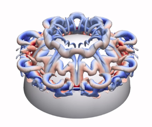
Finally, figure 10 shows the 3-D flow dynamics resulting from a  $D/d=2$ hemisphere based vortex ring collision (see supplementary movie 5). The overall flow developments reveal that the biggest distinction between this and earlier
  $D/d=0.5$ and 1 configurations is that the present primary vortex ring does not reach and interact with the wall boundary layer at all. Instead, the entire flow dynamics plays out along the hemispheric surface before it transits to incoherence. Formations of the secondary, tertiary and second tertiary vortex rings resulting from the primary vortex ring collision with the hemispheric surface resemble qualitatively that seen for the secondary vortex ring observed in the
  $D/d=1$ hemisphere configuration, except that they are now produced by multiple consecutive hemisphere boundary layer separations as shown in figures 10(a–d). Similarly, figures 10(e,f) also show that the secondary vortex ring becomes unstable and wavy after it leapfrogs over and is being entrained by the primary vortex ring. Unlike the
  $D/d=1$ hemisphere configuration, however, where the wavy secondary vortex ring produces multiple loops that extend downwards towards the wall, figures 10(g,h) show that the present wavy secondary vortex ring moves upstream and away from the hemispheric surface instead. Remarkably, the secondary vortex ring retains its moderately wavy outline thereafter until the onset of flow incoherence. The main reason behind this observation can be discerned in figures 10(g,h), where the tertiary vortex ring hardly interacts with the wavy secondary vortex ring after the former is entrained by the primary vortex ring, due to the secondary vortex ring moving away from the hemisphere. This is in stark contrast to the
  $D/d=1$ hemisphere configuration.

Figure 10. Vortex ring structures and 3-D vortex dynamics produced by  $D/d=2$ hemisphere based vortex ring collision, for (a)
  $\tau =0.95$, (b)
  $\tau =1.80$, (c)
  $\tau =2.20$, (d)
  $\tau =2.50$, (e)
  $\tau =2.90$, (f)
  $\tau =3.20$, (g)
  $\tau =3.50$, (h)
  $\tau =3.80$, (i)
  $\tau =4.10$, (j)
  $\tau =4.40$.
Furthermore, it should be noted that the second tertiary vortex ring first observed in figure 10(f) grows in physical size and is subsequently entrained by the primary vortex ring as shown in figure 10(h). This leads to an interesting situation where the entrained secondary, tertiary and second tertiary vortex rings maintain their large-scale coherence relatively well, despite the tertiary vortex ring developing some slight waviness, and loops of the second tertiary vortex ring beginning to entangle round the primary vortex ring. It should also be highlighted that close proximity of the secondary and tertiary vortex rings to the hemispheric surface leads to localized hemisphere boundary layer separations that manifest into small regular vortex loops. In the next time instance shown in figure 10(i), the wavy secondary vortex loop is now displaced further away from the hemisphere top, and the small regular vortex loops are now beginning to entangle with it. The tertiary vortex ring can also be seen to move towards and up the hemispheric surface while forming regular loops at the same time. On the other hand, bottom loops from the second tertiary vortex ring loops become more entangled around the primary vortex ring, while the top main loops move up and towards the hemisphere surface. In fact, subsequent flow behaviour observed in figure 10(j) portrays a situation whereby all the secondary and tertiary vortex rings/loops move upstream while interacting with one another. On the other hand, the top loops of the second tertiary vortex ring are spreading radially outwards, while its bottom loops are moving downstream instead. From here on, the flow begins to transit to incoherence, with increased interactions between the numerous vortex structures.
To better understand the more convoluted vortex dynamics, figure 11 shows the vorticity fields for the same  $D/d=2$ hemisphere extracted from supplementary movie 6, and it is clear that all immediate flow developments are indeed limited to the larger hemispheric surface. Vortex cores associated with the secondary vortex ring and three tertiary vortex rings can be observed to form one after another in figures 11(c–g), with each one forming progressively further downstream along the hemispheric surface. This deviates from the smaller
  $D/d=0.5$ and 1 hemispheres discussed earlier, and as such, flow developments for the largest hemisphere are the most distinct of all three studied here. In particular, the subsequent upstream movement of the secondary vortex ring and the entrained small vortex loops produced by the hemisphere boundary layer separation can be discerned clearly in figures 11(i,j). In fact, this observation is reminiscent of the rebounding behaviour exhibited by the secondary vortex ring produced by vortex ring collision with a
  $D/d=2$ round cylinder in New & Zang (Reference New and Zang2017). It can be appreciated that the secondary and tertiary vortex ring cores become increasingly smaller with time, as their ring diameters increase with their motions along the hemispheric surface. This thus suggests that a larger hemisphere could confer additional vortex-stretching effects, much like what had been reported by New & Zang (Reference New and Zang2017) for round cylinder-based vortex ring collisions.

Figure 11. The 2-D vorticity fields associated with  $D/d=2$ hemisphere based vortex ring collision, for (a)
  $\tau =0.95$, (b)
  $\tau =1.80$, (c)
  $\tau =2.20$, (d)
  $\tau =2.50$, (e)
  $\tau =2.90$, (f)
  $\tau =3.20$, (g)
  $\tau =3.50$, (h)
  $\tau =3.80$, (i)
  $\tau =4.10$, (j)
  $\tau =4.40$.
It should be noted that a recent study by Mishra et al. (Reference Mishra, Pumir and Ostilla-Mónico2021) elaborated upon the effects of primary vortex ring Reynolds number and core thickness on the formations and behaviour of the secondary and tertiary vortex rings. That study shows that the use of a significantly thicker vortex ring core thickness will lead to more stable vortex ring structures and collision behaviour with less flow instabilities. Hence increasing the core thickness beyond the initial core to vortex ring radius ratio 0.1 used here significantly could lead to tangibly more stable secondary and tertiary vortex ring behaviour with fewer azimuthal instabilities. However, as the emphasis here is to conduct a more comprehensive and thorough analysis of the simulation results based on a moderately laminar vortex ring at a single Reynolds number first, its effects will be considered in future studies. On the other hand, while the effects of core thickness variations are not investigated specifically here,  $D/d=1$ hemisphere based vortex ring collision was simulated based on a specific discharge velocity model proposed by Danaila, Vadean & Danaila (Reference Danaila, Vadean and Danaila2009), and compared to the present LES results later. As the primary vortex ring core thicknesses differ between the two approaches due to the use of different initializations, the influences of core thickness upon the collision behaviour may then be inferred.
3.2. Vortex core trajectories and formation locations
Figure 12 shows the vortex core trajectories extracted for all three hemispheres here, with results for the same vortex ring colliding against a flat wall (New et al. Reference New, Shi and Zang2016) included for comparison. To allow better understanding, small arrows are used to indicate the starting points of the vortex core trajectories, with the arrows coloured accordingly to primary, secondary, tertiary, and second and third tertiary vortex cores, as indicated in the legend. Briefly summarizing, results for the flat-wall-based vortex ring collision show that the primary vortex cores move radially outwards upon the collision and incur a slight rebound, before continuing to move radially outwards at a much-reduced pace. The secondary vortex cores, on the other hand, leapfrog over and are subsequently entrained by the primary vortex cores. Subsequently, they reside well within the primary vortex ring and move towards the collision axis along the flat wall. Only one set of tertiary vortex cores is produced, and while they leapfrog over the primary vortex cores, they are not fully entrained by the primary vortex cores but move towards the collision axis instead.

Figure 12. Vortex core trajectories for the present vortex ring collisions upon (a) a flat wall, (b) a  $D/d=0.5$ hemisphere, (c) a
  $D/d=1$ hemisphere and (d) a
  $D/d=2$ hemisphere.
For the  $D/d=0.5$ hemisphere shown in figure 12(b), the presence of the hemisphere confers a few discernible changes to the vortex core trajectories despite its small physical size. First, the primary vortex cores do not spread out radially along the wall as much as in the flat wall scenario. Second, the secondary vortex cores do not move towards the collision axis after entrainment by the primary vortex ring cores, likely due to blockage by the hemisphere. Instead, they move beneath the primary vortex cores before entangling the primary vortex ring at regular intervals, as seen in figure 6(h) earlier. The entanglement behaviour would then lead to the more limited radial movements of the primary vortex ring cores noted in the figure. While the tertiary vortex core trajectory remains quite similar to the flat wall configuration during the early stages, it ceases to move towards the collision axis after some time. Hence it is clear that the presence of a moderately small hemisphere imposes adverse pressure gradient conditions closer to the collision axis. Despite these differences, however, vortex core trajectories (and thus the vortex dynamics that underpin them) for flat wall and
  $D/d=0.5$ hemisphere configurations remain broadly comparable, due primarily to the fact that all the various vortex ring structures in the latter configuration continue to interact with the wall more than the small hemisphere.
As the hemisphere size increases to  $D/d=1$ as shown in figure 12(c), the primary vortex cores translate further away from the collision axis after it interacts with the hemisphere. On the other hand, secondary vortex cores are now formed along the hemispheric surface instead of the wall. Hence they are now further away from the wall, even though they exhibit relatively similar trajectory trends when they are being entrained by the primary vortex cores. One interesting observation is that the secondary vortex cores eventually return to the hemispheric surface, relatively close to the location where they first form. In addition, the tertiary vortex cores are now being entrained by the primary vortex cores after they are formed along the wall, in contrast to the flat wall and
  $D/d=0.5$ hemisphere configurations. As for the second tertiary vortex cores after they are formed, they move upstream and closer towards the collision axis in a diagonal fashion. Note that they are the only set of vortex cores that are not entrained by the primary vortex cores.
As for the largest  $D/d=2$ hemisphere depicted in figure 12(d), the vortex core trajectories are now much more convoluted, since all vortex rings only interact with or originate from the hemispheric surface. Starting with the primary vortex cores, they move downstream along the hemispheric surface after the collision instead of moving laterally away from it, a clear departure from the preceding configurations. The secondary vortex cores are once again entrained by the primary vortex cores shortly after they are formed and travel to the vicinity where they first formed, before moving upstream and towards the collision axis. This is not observed for the other three previous configurations, and the upstream movement is much faster than the inward motion towards the collision axis. Interestingly, the formations and trajectories of all three sets of tertiary vortex cores are very similar, with one set forming progressively more downstream along the hemispheric surface than the previous set, before eventually getting entrained by the primary vortex cores.
A larger hemisphere naturally presents a larger blockage and higher adverse pressure gradient to the primary vortex ring as the latter translates towards the former. To aid better understanding, figure 13 shows the variations in the primary vortex ring translational velocity,  $u/u_{t}$, with respect to time
  $\tau$, as it approaches and collides with the present hemispheres and flat wall. Note that the results were extracted from when the primary vortex ring is
  $1.5d$ upstream of the flat wall or hemisphere top. Additionally, figure 13 includes results up to the point when the translational velocity is zero, though that need not necessarily mean that the primary vortex ring has reached the flat wall, since that is not the case for the
  $D/d=2$ hemisphere. For the sake of comparisons, the result for a primary vortex ring translating freely in a quiescent environment is also included, and its translation velocity can be observed to undergo a relatively gentle and linear reduction throughout. As for the flat wall scenario, the primary vortex ring incurs faster velocity reductions and earlier collisions than the hemisphere scenarios. For the
  $D/d=0.5$ hemisphere, the translational velocity reduction trend is quite similar, although the primary vortex ring collides with the flat wall later due to the hemisphere boundary layer formation and their subsequent interactions.

Figure 13. Variations in the primary vortex ring translation velocity as it gradually approaches and eventually collides with the  $D/d=0.5$, 1 and 2 hemispheres.
On the other hand, the use of larger hemispheres leads to more interesting outcomes, where the translational velocity of the primary vortex ring undergoes two distinct linear reduction stages. For instance, up until the time when the primary vortex ring actually interacts with the  $D/d=1$ hemisphere, the slope of its translational velocity reduction is estimated to be approximately
  $s_{1}=-0.18$. However, the slope magnitude increases to
  $s_{2}=-3.2$ after the primary vortex ring begins to interact with the separated hemisphere boundary layer. The situation is similar for the
  $D/d=2$ hemisphere, where the slopes are approximately
  $s_{3}=-0.35$ and
  $s_{4}=-3.3$ before and after the primary vortex ring interacts with the separated hemisphere boundary layer, respectively. It should be highlighted that the primary vortex ring takes the shortest time to reach zero translation velocity here, as figures 10 and 11 show the primary vortex ring interacting only with this hemisphere without reaching the flat wall. It is interesting to note that
  $s_{3}$ is almost twice
  $s_{1}$ when the hemisphere size doubles from
  $D/d=2$ to
  $D/d=1$, which reflects the expectedly larger adverse pressure gradient facing the primary vortex ring when a larger hemisphere is used. What is intriguing is that regardless of whether a
  $D/d=1$ or
  $D/d=2$ hemisphere is used, the translational velocity reduction rates are practically the same after the primary vortex ring has started interacting with the separated hemisphere boundary layers. This suggests that adverse pressure gradient plays little role in the primary vortex ring translational velocity reductions during this collision stage. Instead, the formations of the secondary and tertiary vortex rings, as well as their subsequent interactions with the primary vortex ring and amongst themselves, would have exerted far more influence.
Next, circulation changes in the primary, secondary and tertiary vortex cores will be discussed, and results for hemisphere and flat wall scenarios are shown in figure 14. Note that the instantaneous circulation levels  $\varGamma$ for all vortex cores in the figure are non-dimensionalized by the primary vortex ring core circulation at
  $\varGamma _{\tau =0.95}$, where the vortex ring has become more fully developed. Figure 14(a) shows the primary vortex core undergoing increasingly greater reductions in its circulation as it approaches and collides with the flat wall. Thereafter, its circulation level undergoes small reductions as it begins to entrain the secondary and tertiary vortex cores formed during the collision process, before it declines sharply after its vortex cores break down rapidly. As for the hemispheres, figures 14(b–d) show that while the primary vortex core circulations undergo faster reductions during the collision, there exist momentarily recoveries as compared to the flat wall. In particular, post-collision circulation recovery is the highest for the
  $D/d=1$ hemisphere and could be attributed to the larger circulation reduction when the primary vortex ring core collides with the hemisphere before encountering the flat wall later. Interestingly, the maximum primary vortex core circulation level after recovering from hemisphere/flat-wall-based collisions decreases when a larger hemisphere is used. The larger circulation drop is likely due to higher energy dissipation caused by the hemispheric surfaces, for which the primary vortex cores are in close proximity over longer distances. Initial secondary and tertiary vortex core circulation levels for the flat wall as shown in figure 14(a) are relatively similar at approximately
  $\varGamma /\varGamma _{\tau =0.95}=0.2$, shortly after they are formed, though they decrease eventually as they are entrained by and interact with the primary vortex cores. An interesting observation is that the secondary vortex core initial circulation level starts out lower but increases gradually to a maximum of approximately
  $\varGamma /\varGamma _{\tau =0.95}=0.2$ as the flow develops for hemisphere-based collisions. Intuitively, hemispheric surfaces produce comparatively lower adverse pressure gradients that allow secondary vortex cores to grow more gradually and exhibit such an outcome. Finally, tertiary vortex core circulation levels are close to those of the secondary vortex cores, before dissipating gradually with time.

Figure 14. Variations in the primary, secondary and tertiary vortex ring circulations as the primary vortex ring collides with (a) a flat wall, (b) a  $D/d=0.5$ hemisphere, (c) a
  $D/d=1$ hemisphere, and (d) a
  $D/d=2$ hemisphere. Approximate points of collision or contact between the primary vortex ring and the hemisphere/wall are indicated for clarity.
Since the primary geometrical difference between round cylinder and hemisphere based collisions will be the absence of straight edges and presence of a flat wall in the latter, this is a good opportunity to discern how the vortex formation locations differ along the convex surfaces between the two geometries. Angular locations relative to the collision axis where all discernible secondary and tertiary vortex cores are formed along the convex cylindrical/hemispheric surfaces ( $\theta$ and
  $\phi$, respectively) were extracted from the experimental and LES results of New & Zang (Reference New and Zang2017) and New et al. (Reference New, Gotama and Vevek2021), respectively, and they are plotted together with those obtained from the present study and presented in figure 15. In particular, it should be highlighted that while the primary vortex ring Reynolds numbers used by these studies are either
  $Re_{d}=Ud/\nu =2000$ or 4000, New et al. (Reference New, Shi and Zang2016) and New & Zang (Reference New and Zang2017) had earlier noted that the use of the
  $Re_{d}=4000$ primary vortex ring leads to a temporally faster flow behaviour, rather than affecting the fundamental vortex dynamics. Also, primary vortex ring initialization procedures here are the same as in New et al. (Reference New, Gotama and Vevek2021).

Figure 15. Comparisons of (a) secondary vortex core and (b) tertiary vortex core formation locations between earlier and present experimental/numerical studies, as well as secondary and tertiary vortex cores relative to (c) vortex formation locations and (d) their relative changes for the same cylinder/hemisphere.
Comparing the round cylinders to the present hemisphere configurations in figure 15(a), hemispheres lead to faster secondary vortex core formations (i.e. smaller  $\theta$), with approximately 0.23–0.36 radian reductions. A similar situation can be observed for the various tertiary vortex core formation locations shown in figure 15(b), where the earlier simulations by New et al. (Reference New, Gotama and Vevek2021) consistently underpredicted the formation angles (i.e. smaller
  $\phi$), as compared to their experimental counterparts in New & Zang (Reference New and Zang2017) previously. Compared with the average trend estimated by the previous experimental and LES studies, however, the present
  $D/d=2$ hemisphere results in a further reduction of approximately 0.33 radians in the first tertiary vortex core formation location. Subsequent formations of the second and third sets of tertiary vortex cores can be seen to occur at progressively larger angles, though they all remain smaller than those produced by the cylinders. This could be explained by the presence of a flat wall for the hemispheres here, which presents higher adverse pressure gradients in the streamwise direction and likely leads to earlier vortex core formations. For the earlier cylinder scenarios, however, there is no flow blockage other than the cylinders themselves, and the primary vortex rings are thus able to wrap themselves around the cylindrical surfaces and undergo vortex stretching, before the secondary and tertiary vortex rings are formed.
Further comparisons on the various vortex core formation locations up to the third tertiary vortex cores for both cylinder and hemisphere configurations are presented in figures 15(c,d). Note that clear formations of only one set of tertiary vortex cores could be observed for cylinders from the earlier studies, and that only the  $D/d=2$ hemisphere results in all the secondary and tertiary vortex cores forming off the hemispheric surface. Returning to figure 15(c), on top of the clear dependency of the vortex core formation locations upon the diameter ratio, persistently earlier secondary and tertiary vortex core formation locations for the
  $D/d=2$ hemisphere as compared to its
  $D/d=2$ cylindrical counterpart can be observed. Additionally, the vortex formation locations tend towards an asymptotic level after the third tertiary vortex cores for the
  $D/d=2$ hemisphere. This can be discerned better in figure 15(d), where changes in the vortex formation locations from each vortex core type to another are presented.
3.3. Vortex flow models
Based on the detailed simulation results discussed earlier, interpretations of the fundamental flow mechanisms and how they are influenced by the diameter ratio will now be presented in figures 16–18. Note that only key coherent vortex ring structures and behaviour will be depicted at different flow stages in the vortex flow models, as the emphasis will be on the more important flow changes to the coherent flow structures.
Starting with figure 16(a), where the vortex flow model for the  $D/d=0.5$ hemisphere is shown with the primary vortex ring translating towards the hemisphere, the interpreted flow mechanisms do not differ significantly from those associated with the flat wall reported previously due to the relatively small hemisphere. The secondary vortex ring forms as shown in figure 16(b) after the wall boundary layer separates, before it leapfrogs over and gets entrained within the primary vortex ring inner confines seen in figure 16(c). A tertiary vortex ring also forms after a second wall boundary layer separation, and in particular, a small hemispheric vortex ring will form close to the hemisphere–wall junction. This hemispheric vortex ring arises from hemisphere boundary layer separation induced by the primary vortex ring moving towards the wall, and convects upstream along the hemispheric surface. By this time, regular secondary vortex ring segments would be entrained by the primary vortex ring, manifesting as secondary vortex loops wrapping themselves around the latter as shown in figure 16(d). As the tertiary vortex ring leapfrogs over and is entrained by the primary vortex ring, it interacts with the secondary vortex ring segments within the latter before the flow becomes incoherent, much like flat-wall-based collisions.

Figure 16. Vortex flow model interpreted for a vortex ring colliding upon a  $D/d=0.5$ hemisphere.
Next, the vortex flow model for the  $D/d=1$ hemisphere is presented in figure 17, where the hemisphere and primary vortex ring sizes are now comparable. As the primary vortex ring translates towards the hemisphere as shown in figure 17(a), its increasing proximity causes the hemisphere boundary layer to separate and produce the secondary vortex ring as shown in figure 17(b). Thereafter, the secondary vortex ring leapfrogs over the primary vortex ring and moves towards the inner confines of the primary vortex ring. However, a blockage posed by the larger
  $D/d=1$ hemisphere within the primary vortex ring means that the secondary vortex ring behaviour deviates from that postulated for the smaller
  $D/d=0.5$ hemisphere. In this case, the secondary vortex ring develops wavy instabilities as it moves closer to the hemisphere, before it takes on a regular wavy outline as shown in figure 17(c). In fact, interactions between the secondary vortex ring and the larger hemisphere here not only make the waviness manifest more quickly but also lead to minor wavy hemisphere boundary layer separations, the latter of which develop into regular vortex loops that move towards the collision axis later. Figure 17(d) onwards shows that much of the wavy secondary vortex ring would stay adjacent to the hemisphere as the flow develops further due to the blockage by the hemisphere, even when its segments begin to entangle around the primary vortex ring later in figure 17(e). This is due to the tertiary vortex ring being formed off the wall boundary layer separation depicted in figure 17(c), and leapfrogging over the primary vortex ring to reside between the primary and secondary vortex rings as shown in figures 17(d) and 17(e), respectively. Subsequently, a myriad of interactions between the primary, secondary and tertiary vortex rings would render the flow incoherent. Finally, the top segments of the wavy hemispheric vortex ring move towards the collision axis along the hemisphere top, though this is not sketched out beyond figure 17(e) to avoid clutter.

Figure 17. Vortex flow model interpreted for a vortex ring colliding with a  $D/d=1$ hemisphere. Note that for the sake of clarity, only half of the primary and second tertiary vortex rings are shown in (e), so as to better reveal the other vortex ring structures located closer to the hemisphere.
Finally, figure 18 shows the vortex flow model for the  $D/d=2$ hemisphere, where in line with the earlier results, formations of new vortex ring structures and flow dynamics are shown limited to along the hemispheric surface. Figure 18(a) shows the relatively smaller vortex ring translating towards the larger hemisphere, where it collides close to the hemisphere top and leads to the formation of the secondary vortex ring, as depicted in figure 18(b). As the secondary vortex ring leapfrogs over the primary vortex ring, the continuing movement along the hemispheric surface by the latter ensures that a tertiary vortex ring forms shortly, as shown in figure 18(c). Subsequently, figure 18(d) shows the secondary vortex ring becoming wavy, much like what had been postulated for the
  $D/d=1$ hemisphere earlier, as well as the tertiary vortex ring leapfrogging over the primary vortex ring such that it resides between the secondary and primary secondary vortex rings depicted in figure 18(d). Rather than moving downwards along the hemisphere like what had been put forward for the
  $D/d=1$ hemisphere, the present wavy secondary vortex ring reduces in diameter, increases in waviness, and moves upstream as shown in figures 18(d–f) instead, in accordance with the results. Similar to the
  $D/d=1$ hemisphere, proximity of the secondary vortex ring to the hemisphere leads the hemisphere boundary layer to separate and produce a small hemispheric vortex ring/loop, as depicted in figure 18(e). Due to influences from the wavy secondary vortex ring, it too becomes wavy and entangles with the former, as shown in figure 18(f). During this time, the primary vortex ring continues to move down the hemisphere, which leads a second tertiary vortex ring to form and go through similar leapfrogging processes as before.

Figure 18. Vortex dynamics interpretations for a vortex ring colliding with a  $D/d=2$ hemisphere. Similar to the approach used in figure 17(e), only half of the primary and third tertiary vortex rings are shown in (f) to better visualize other vortex ring structures located closer to the hemispheric surface.
Returning to the first tertiary vortex ring, it becomes progressively wavy as it approaches the hemispheric surface. As for the second tertiary vortex ring, eventually it lodges itself between the first tertiary and primary vortex ring, as shown in figure 18(f). Unlike the secondary and first tertiary vortex rings, which are not entangled around the primary vortex ring due to the latter's movements down the hemisphere, regular wavy second tertiary vortex ring segments do get entangled with the primary vortex ring. This can be explained by the earlier postulation that the primary vortex ring will be moving at a progressively slower velocity as the local hemispheric diameter increases, which at some point allows the second tertiary vortex ring to ‘intercept’ and interact with it. Finally, figure 18(f) depicts the primary vortex ring leading to yet another boundary layer separation along the hemisphere, to produce a third tertiary vortex ring. Based on the present vortex flow model, it is hypothesized that for a hemisphere that possesses a diameter that is sufficiently larger than the vortex ring diameter (i.e.  $D/d\geq 2$ under the present test conditions), the key flow mechanism associated with a head-on vortex ring collision is one that sees repeated hemisphere boundary layer separations and repeated formations of other secondary/tertiary vortex rings of opposite rotational sense, caused by the primary vortex ring as it translates along the hemisphere. This recurring behaviour will cease eventually when the primary vortex ring becomes sufficiently weakened, caught up by and interacting with the last vortex ring structure that it induces.
Interestingly, this suggests that for larger surface-mounted hemispheres where the presence of the wall may be neglected, or isolated spheres, the number of secondary and tertiary vortex ring structures induced by the primary vortex ring is strongly dependent upon how well the primary vortex ring outpaces the various vortex rings that it induces continuously along the hemisphere. Since a larger hemisphere or sphere poses a larger blockage and in turn decelerates the translation velocity of the primary vortex ring faster, the primary vortex ring will not be able to induce as many secondary and tertiary vortex rings along the hemispheric/spherical surface before the last one entangles with it, rendering it sufficiently incoherent to proceed any further. As such, it is hypothesized that there exists an inverse relationship between the hemisphere/sphere size and the number of vortex ring structures induced along larger hemispheric/spherical surfaces. For instance, a  $D/d>2$ hemisphere is likely to see a lower number of tertiary vortex rings formed along its surface as compared to the
  $D/d=2$ scenario, as the primary vortex ring will not outpace the tertiary vortex rings as well as when the hemisphere is smaller, and would eventually be caught up, entangled with, and rendered incoherent by the last tertiary vortex ring formed. This is consistent with flat-wall-based collisions, where typically, only one secondary and one tertiary vortex ring are observed under similar conditions.
This line of thought will in fact be in gross agreement with the earlier study by New & Zang (Reference New and Zang2017). In that study, round-cylinder-based collisions revealed that, similar to the present collisions, key vortex dynamics are progressively limited to the upstream regions of the convex surfaces as the cylinder size increases. In particular, significant movements of the secondary vortex rings towards the collision axis and upstream region after the collisions were observed for  $D/d\geq 2$ cylinders in that study, where their upstream movements are much smaller at
  $D/d=4$ than at
  $D/d=2$. While the exact geometries of that study and the present one are different, the dominant presence of convex surfaces in both geometries reinforces the notion that key aspects of the flow will be similar. Therefore, what is likely to happen when the present hemisphere size exceeds
  $D/d=2$ is that increasingly, the collision behaviour will be restricted to the hemisphere top, with the secondary and tertiary vortex rings moving progressively more towards the collision axis and less towards the downstream direction. As the size increases further and approaches an asymptotical flat wall configuration, eventually collision behaviour will reconcile with what had been reported typically for flat wall scenarios previously.
3.4. Comparisons with specific discharge velocity models
Results presented thus far have made use of vortex rings initialized with a Gaussian function without the need to compute the flow within a cylinder or model the cylindrical-slug flow characteristics that are typically involved in experimental vortex ring generations. While the vortex ring models and formulations used in the present study are in line with those adopted by earlier simulation-based studies, it should be noted that Danaila et al. (Reference Danaila, Vadean and Danaila2009) had proposed another approach that seeks a good compromise between using simplistic Gaussian-based vortex rings and those modelled after cylindrical-slug flows. In particular, specific discharge velocity (SDV) models based on either transient developments of the centreline velocity, or boundary layer characteristics at the cylinder exit, were both mooted to describe the exit conditions of a piston/cylinder set-up to generate laminar vortex rings numerically. To compare any flow differences arising from the use of the present and SDV approaches for the present hemisphere-based collisions, a single SDV-based simulation using centreline velocity variations was conducted according to Danaila et al. (Reference Danaila, Vadean and Danaila2009) for a  $D/d=1$ hemisphere based collision. Note that the cylinder exit has to be adjusted further upstream of the hemisphere at
  $3.5d$ away, such that the circulation of the fully developed SDV-based vortex ring matches that of the present Gaussian-based vortex ring for better comparisons. Naturally, this led to corresponding increases in the non-dimensionalized timings of the results that will be presented later. Additionally, the SDV-based vortex ring initial translational velocity was adjusted to be almost similar to that of the Gaussian-based vortex ring.
Figure 19 shows the vortex ring structures and dynamics for the SDV-based  $D/d=1$ hemisphere based collision, while figure 20 shows the corresponding 2-D vorticity results. Note that these results were selected by matching figure 20 vorticity results with those shown in figure 9 earlier, as much as possible, and all
  $\lambda _2$-criterion cut-off values and colour legends remain the same. Inspecting figure 19 will show that as the collision progresses up to figure 19(e) after the secondary vortex ring leapfrogs over the primary vortex ring and converges towards the hemisphere, it does not transit into a wavy state like figure 8(e) previously. In fact, other than some very minor segmentations of the vortex ring filament, which become apparent only much later during the collision, the secondary vortex ring is far more stable than can be observed in figure 8. The same can be said for the tertiary vortex rings, as shown in figure 19(h) onwards. The end result is a collision behaviour that is almost devoid of any significant azimuthal instabilities for the various vortex ring structures, in contrast to the behaviour depicted in figure 8 earlier. As such, the secondary vortex ring in figure 20 can be observed to move far more upstream than its counterpart in figure 9 after interacting with the hemisphere, as it interacts less with the primary and tertiary vortex rings. Apart from that, however, comparisons between results obtained from SDV- and Gaussian-based vortex ring based approaches reveal that there exist good agreements in larger-scale coherent vortex ring formations, structures and dynamics.

Figure 19. Vortex ring structures and 3-D vortex dynamics produced by a  $D/d=1$ hemisphere based vortex ring collision modelled using the SDV approach, for (a)
  $\tau =1.30$, (b)
  $\tau =2.20$, (c)
  $\tau =3.00$, (d)
  $\tau =3.70$, (e)
  $\tau =4.70$, (f)
  $\tau =5.50$, (g)
  $\tau =6.20$, (h)
  $\tau =7.40$, (i)
  $\tau =8.10$, (j)
  $\tau =9.20$.

Figure 20. The 2-D vorticity fields associated with a  $D/d=1$ hemisphere based vortex ring collision modelled using the SDV approach, for (a)
  $\tau =1.30$, (b)
  $\tau =2.20$, (c)
  $\tau =3.00$, (d)
  $\tau =3.70$, (e)
  $\tau =4.70$, (f)
  $\tau =5.50$, (g)
  $\tau =6.20$, (h)
  $\tau =7.40$, (i)
  $\tau =8.10$, (j)
  $\tau =9.20$.
While the Gaussian-based vortex ring and SDV approaches in generating the vortex rings are dissimilar, the fact that the vortex ring circulation and initial translational velocity are almost the same between the two approaches means that the more tangible and interesting difference between them will be the vortex ring core thickness. To probe further, fully developed SDV-based vortex ring core thickness was estimated based on the procedures outlined by Archer, Thomas & Coleman (Reference Archer, Thomas and Coleman2008) and found to be approximately 1.64 times that of its Gaussian-based counterpart. Recall from earlier that primary vortex rings with thicker core thicknesses are significantly more stable, with little deformations to both them and secondary vortex ring filaments during a flat-wall-based collision (Mishra et al. Reference Mishra, Pumir and Ostilla-Mónico2021). Since the SDV-based vortex ring has a significantly thicker core thickness, it is expected that the primary, secondary and tertiary vortex ring structures would be more stable, incur lesser deformations, and produce a smaller number of azimuthal instabilities. Comparisons between the isosurface results in figures 8 and 19 show that is indeed the case here, and offer some early insights into how hemisphere-based vortex ring collisions will differ if the primary vortex ring has a thicker core thickness.
4. Conclusions
An LES study on wall-mounted hemisphere based vortex ring collisions was conducted for diameter ratios  $D/d=0.5\unicode{x2013}2$. Results show that a
  $D/d=0.5$ hemisphere results in a flow field that is reminiscent of a flat-wall-based collision, where secondary and tertiary vortex rings result from wall boundary layer separations. For a
  $D/d=1$ hemisphere, secondary and tertiary vortex rings are formed by sequential hemisphere and wall boundary layer separations, respectively, while a
  $D/d=2$ hemisphere will see all secondary and tertiary vortex rings forming from hemisphere boundary layer separations only. As such, the largest hemisphere here limits the key vortex dynamics and structures to manifest along the hemisphere only, with the wall imparting negligible flow influences. Additionally, comparisons of the vortex dynamics and vortex core trajectories reveal both similarities and differences between hemisphere and round-cylinder-based collisions. While there are good agreements in how the diameter ratio affects the vortex formation locations for both hemispheres and cylinders, comparisons also show that secondary and tertiary vortex rings tend to form at smaller angular locations along the hemisphere than for the cylindrical surface at the same diameter ratio. Primary vortex ring translational velocity results show that flat wall and
  $D/d=0.5$ hemisphere based collisions yield nonlinear velocity reductions until the translation velocity reaches zero. In contrast,
  $D/d=1$ and 2 hemisphere based collisions produce two distinct linear velocity reduction stages before the translation velocity reaches zero. Additionally, variations in the circulations for the different vortex ring structures as they undergo various key vortical changes are also compared. In particular, 3-D vortex flow models are constructed to enable better appreciation of the transient vortex dynamics and genesis of the secondary and tertiary vortex rings when the diameter ratio increases from
  $D/d=0.5$ to
  $D/d=2$. Furthermore, they also provide important insights into and understanding of how the primary vortex ring will continue to produce more tertiary vortex rings along a sufficiently large hemisphere, as long as no tertiary vortex ring interferes with or disrupts its continual movements. Additionally,
  $D/d=1$ hemisphere based collision was simulated based on an SDV approach and compared to the LES approach, with the significantly more stable vortex ring developments for the former attributed to the thicker primary vortex ring core thickness produced by the SDV model. Finally, the present findings provide good understanding that could underpin future studies involving other hemisphere-based collision scenarios, such as non-coaxial or multiple hemisphere based collisions with different separation distances to simulate uneven bumpy walls.
Supplementary movies
Supplementary movies are available at https://doi.org/10.1017/jfm.2024.13.
Acknowledgements
The authors gratefully acknowledge support for the present study from the School of Mechanical and Aerospace Engineering, Nanyang Technological University and VOMMA (Shanghai) Technology Co. Ltd. Additionally, computational resources provided by National Supercomputing Centre, Singapore (https://www.nscc.sg), for the study are gratefully acknowledged. In particular, T.H.N. would like to express his deep appreciation for the patience shown by his collaborators for their other joint work.
Funding
Financial support for the present study was provided partially by VOMMA (Shanghai) Technology Co. Ltd (grant no. VOMMA 04OIS000227C160).
Declaration of interests
The authors report no conflict of interest.
Data availability statement
The data that support the findings of this study are available from the corresponding author upon reasonable request.


 Open access