


1. Introduction
Over the last 20 years, tsunami inundation of coastal urban areas has led to more than 200 000 deaths due to building failure and floating debris. These humanitarian disasters have led to greater efforts to improve building designs in susceptible regions through a better understanding of force loadings. The challenge of understanding tsunami inundation of urban areas is due to the free-surface flow being characterised by a long period and the geometrical complexity of buildings and obstructions. One way to meet this challenge is by studying simplified problems, such as how the free-surface interaction with a single body affects a steady channel flow. This idealised set-up can act as a conceptual building block for more complex multiple-body interactions.
The experimental observations of the steady flow past a square cylinder in a channel by Qi, Eames & Johnson (Reference Qi, Eames and Johnson2014) showed two distinct flow states: a subcritical flow state (characterised by an upstream and a downstream subcritical flow) and a choked state (characterised by a transition from a subcritical upstream flow to a supercritical downstream flow). This is represented in figure 1(a), and the idealised set-up is shown in figure 1(b), where the square cylinder is defined by a uniform section ( $b \times b$) that spans the height of the channel. The square cylinder was mounted onto a rigid rod and connected to two calibrated load cells in order to infer the forces on the obstruction. In a channel of width
  $w$, this provides a section of the channel with uniform blocking ratio
  $\phi _B = b/w$. The experimental facilities were limited in the flow rate that could be achieved, so while the flow in the absence of the cylinder was supercritical, the presence of the cylinder caused the flow to jump to a choked state. To interpret these observations, Qi et al. (Reference Qi, Eames and Johnson2014) developed a zero-dimensional model that related (in an integral sense) the loss of the momentum flux to an empirical form of the drag force. This gave a relationship between the upstream Froude number (
 $Fr_u$) and downstream Froude number (
 $Fr_d$) of the square cylinder and, together with a hydraulic jump, enabled the choked state to be analysed. At the time, the importance of the supercritical branch was not analysed or appreciated.

Figure 1. (a) Schematic of the relationship between the Froude numbers upstream ( $Fr_u$) and downstream (
 $Fr_d$) of an obstruction, illustrating the subcritical, supercritical and choked states; the band-gap in the Froude number is labelled. (b) A schematic, with notation, of the delta and uniform drag
  $f_D$ representations and the coordinate axes.
Motivated by a need to understand the fundamental interaction between a dam-break flow and a single building, Eames & Robinson (Reference Eames and Robinson2022) developed a one-dimensional (1-D) model that incorporated the distinct effect of blocking and drag, caused by an obstruction, into a nonlinear shallow-water model. An analysis for steady flows identified complex critical states characterised as subcritical, choked and supercritical with a band-gap in terms of the upstream Froude number (figure 1a). Eames & Robinson (Reference Eames and Robinson2022) showed that for unsteady channel flows, specifically a supercritical dam-break flow, the flow had a tendency to lock on to the steady critical flow states. Although the subcritical and choked states have been reported previously, there has been no other direct support for a band-gap in the flow state – a range of  $Fr_u$ for which no steady solution exists – except for an inference made from the supercritical experimental data of Ducrocq et al. (Reference Ducrocq, Cassan, Chorda and Roux2017). Although this range matches the predictions by Eames & Robinson (Reference Eames and Robinson2022), the supercritical branch remains unstudied. The importance of this supercritical branch is underlined by the fact that most inundation flows, created by a dam-break or tsunami, are supercritical. It is therefore essential that these critical states are studied.
In this paper, a computational methodology is adopted to explore free-surface channel flows around an obstruction, with the flow properties varying from subcritical to supercritical states. A standard open-source software is used that incorporates a number of volume-of-fluid solvers that can accommodate free-surface deformation and breaking. The numerical model used in this study is described in § 2. The results for a blocking ratio of  $\phi _B=0.2$ are first discussed in detail in § 3, covering the flow field, flow state (
 $Fr_u$,
  $Fr_d$), pressure field and total force. The general influence of the blocking ratio is discussed in § 4, before conclusions are drawn in § 5.
2. Mathematical model
The problem is posed simply: the uniform free-surface flow past a square cylinder ( $b \times b$ plan), fixed in a channel (of width
  $w$) and spanning the channel height, is considered (figure 1b). The blocking ratio
  $\phi _B$ is defined to be
  $b/w$. The flow in the computational domain is initialised with a uniform horizontal flow
  $u_0$ and water height
  $h_0$ (set at
  $h_0=0.1$ m), giving an initial Froude number of
  $Fr_0 = u_0/\sqrt {g h_0}$ and a Reynolds number of
  $Re = u_0 h_0/\nu \simeq 10^4{-}10^5$.
The three-dimensional (3-D) viscous flow simulations were chosen to match closely the experimental study of Qi et al. (Reference Qi, Eames and Johnson2014). The experimental study consisted of a flow quietening section, followed by a 1 m straining section before meeting a 3 m long testing section flume with channel width  $w = 0.5$ m and height 0.2 m. The cylinder spanned the entire height of the domain, and the front face was located 1.5 m from the inlet. For supercritical flows, the water height rose at the front of the cylinder and generated a long persistent wake pattern. For this reason, the computational domain was chosen to be longer (at 5.0 m) and taller (
 $H_c =0.3$ m) to cope with high Froude numbers. Here, we focus on the flow developed after running for a period of at least 20 s.
2.1. Computational model
Free-surface overturning was anticipated, which meant choosing a computational model that can cope with changes in surface topology. A standard model that can account for this effect is the volume-of-fluid formulation (Hirt & Nichols Reference Hirt and Nichols1981) based on describing the phase as a colour function ( $\alpha$) that takes value 0 for a gas and 1 for a liquid. The fluid properties (e.g. density, viscosity) are described using a scalar
  $\alpha$ that represents the fraction of liquid present in a computational cell. The fluid properties are defined to vary linearly between
  $\alpha =0$ and
  $\alpha =1$, e.g.
  $P= \alpha P_f +(1-\alpha )P_g$, where
  $P$ is a scalar property, such as density (
 $\rho$) or viscosity (
 $\mu$), that takes value
  $P_g$ in the gas and
  $P_f$ in the liquid. The momentum equation, describing the relationship between the evolution of the velocity field
  $u_i$ and pressure
  $p$, is
 \begin{align} \frac{\partial u_i }{\partial x_i}=0, \quad \frac{\partial }{\partial t}(\rho u_i) + \frac{\partial }{\partial x_j} (\rho u_i u_j) ={-} \frac{ \partial p }{\partial x_i} + \frac{\partial }{\partial x_j}(2(\mu+\mu_t)S_{ij}) + \rho g_j + \sigma \kappa\,\frac{\partial \alpha }{\partial x_i}, \end{align}
where  $S_{ij}=({\partial u_i}/{\partial x_j}+{\partial u_j}/{\partial x_i})/2$ is the mean strain rate tensor and
  $g_j$ is the gravitational acceleration. The surface tension is
  $\sigma$, and
  $\kappa$ is the curvature at the interface between air and water. To reduce the influence of numerical diffusion, an interface compression scheme sharpens the gradients of the liquid–gas interface through
 \begin{equation} \frac{\partial \alpha }{\partial t} + \frac{\partial }{\partial x_j} (\alpha u_j) + \frac{\partial }{\partial x_j} (\alpha (1-\alpha) u_j^r) =0, \end{equation}
where  $\boldsymbol {u}^r = \boldsymbol {\nabla } \alpha / |\boldsymbol {\nabla } \alpha |$.
To accommodate the high Reynolds numbers, a turbulence closure is necessary to pick up the additional subgrid-scale processes. Of the many available numerical models, we choose the  $k$–
$k$– $\omega$ turbulence model (Menter Reference Menter1994), which is generally better with lower Reynolds numbers adjacent to walls. This model is based on describing the evolution of the kinetic energy
  $k$ and the rate of dissipation
  $\omega$ through
 \begin{equation} \frac{\partial}{\partial t}(\rho k)+\frac{\partial}{\partial x_j}(\rho u_j k)=\frac{\partial}{\partial x_j}\left((\mu+\mu_t\sigma_k)\,\frac{\partial k}{\partial x_j} \right) + G-\beta^*\rho \omega k, \end{equation}
 \begin{equation} \frac{\partial}{\partial t}(\rho \omega)+\frac{\partial}{\partial x_j}(\rho u_j \omega)=\frac{\partial}{\partial x_j}\left((\mu+\mu_t\sigma_{\omega})\,\frac{\partial\omega}{\partial x_j}\right) + \frac{\gamma G}{\nu_t}-\beta\rho\omega^2+2\rho(1-F_1)\,\frac{\sigma_{\omega^2}}{\omega}\,\frac{\partial k}{\partial x_j}\,\frac{\partial \omega}{\partial x_j}, \end{equation}
where
 \begin{equation} G=\tau_{ij}\,\frac{\partial u_i}{\partial x_j}, \quad \mu_t = \frac{\rho a_1 k}{\max(a_1\omega, SF_2)}. \end{equation}
The coefficients  $a_1,c_1\ {\rm and}\ \beta ^*$ and blending functions
  $F_1\ {\rm and}\ F_2$ are described by Menter (Reference Menter1994).
The computational model is solved using OpenFOAM's interFoam module with the waves2Foam package (Jacobsen, Fuhrman & Fredsoe Reference Jacobsen, Fuhrman and Fredsoe2012) so that the non-reflecting inlet and outlet boundary conditions can be imposed. The turbulence closure model was set to be the default  $k$–
$k$– $\omega$ turbulence model. The non-reflecting inlet condition was applied on the first 0.5 m of the computational domain, while the outlet constraint was applied on the last 0.5 m of the domain. No-slip conditions were applied on the channel and cylinder walls, and on the surface
  $z=0$. On the upper surface of the computational domain, the static pressure is set to a constant and a slip condition is applied. A weak turbulent intensity of
  $0.037\,{\rm m}\,{\rm s}^{-1}$ is applied on the inlet condition. The sensitivity of any results to a turbulence closure model depends on the range of
  $Re$ and the geometry. This is especially true for flow past circular cylinders, where the point of separation can shift dramatically. For flows past buildings with sharp corners, the drag force shows less sensitivity to the turbulence modelling.
The numerical results were compared against a 1-D shallow-water model based on describing the influence of the cylinder on the flow as being through a distributed drag and blocking (see Eames & Robinson Reference Eames and Robinson2022). The relationship between upstream and downstream Froude numbers can be calculated from the steady-state solution (see § 3.1). The relationship between the initial and final states required solving the unsteady shallow-water model until a steady solution was achieved.
2.2. Diagnostic tools
The mean flow was orientated along the  $x$-axis, with the
  $y$-axis being directed across the channel. The main diagnostic was the local Froude number, defined as a function of
  $x\ {\rm and} \ y$ and evaluated as
  $Fr(\boldsymbol {x}) = \bar {u}/\sqrt {g \bar {h}}$ from the depth-averaged speed
  $\bar {u} = ({1}/{\bar {h}}) \int _0^{H_c} u(x,y,z)\,\alpha \,{\rm d} z$ and height
  $\bar {h} = \int _0^{H_c} \alpha \,{\rm d} z$. Upstream of the cylinder, the flow tends to be uniform between the quietening section and cylinder, so that
  $Fr_u$ can be identified from a single value on the centreline. The
  $Fr_d$ value is obtained by averaging across the channel width. The drag force on the cylinder is defined as
 \begin{equation} F_D =\hat{\boldsymbol{x}} \boldsymbol{\cdot} \int_{S_b} ({-}p\boldsymbol{ I} +\boldsymbol{ \tau}) \boldsymbol{\cdot} \hat{\boldsymbol{n}} \,\mathrm{d}S,\end{equation}
where  $S_b$ is the cross-sectional area of the channel domain and
  $\boldsymbol {I}$ is the identity matrix.
When the force is oscillatory, it is necessary to average  $F_D$ over time. A dimensionless drag coefficient can be defined based on either the initial reference state
  $C_{D0} = 2F_D/(\rho b u_0^2 h_0)$ or the final reference state
  $C_{D} = 2F_D/(\rho b u_u^2 h_u)$, based on upstream flow variables.
2.3. Sensitivity tests
The influence of mesh quality was studied with the structured mesh over a computational domain  $5\,{\rm m} \times 0.5\,{\rm m} \times 0.3\,{\rm m}$; the mesh was characterised by
  $770\times 150\times 160$ points in the streamwise, cross-stream and vertical directions. The difference between
  $Fr$ and
  $F_D$ evaluated from 2.5 million and 15.2 million cells was less than 2 %. Some measures, such as the critical values of
  $Fr$, showed less sensitivity to the resolution except close to the choked state. The structure of the flow is described for
  $\phi _B = 0.2$ over the range
  $0< Fr_0\le 3.0$, and the influence of blocking is discussed for the range
  $0.1\le \phi _B\le 0.4$.
3. Drag and blocking
The free-surface flow past the cylinder tends to be locked onto a unique Froude number curve whose branches can be characterised in terms  $Fr_u$ and
  $Fr_d$. The essential feature of this relationship can be understood broadly by studying how the momentum flux (
 $M$) and
  $Fr$ vary along the channel. Numerical interpretation offers an opportunity to analyse these effects in isolation.
3.1. Momentum flux analysis
The streamwise momentum flux ( $M$) and volume flux (
 $q$) are defined in terms of integrals in the
  $yz$-plane:
 \begin{equation} M = \int_A ( \rho u_x^2 +p ) \,{\rm d}A, \quad q =\int_A \rho u_x \,{\rm d} A\Big/\int_A \rho \,{\rm d} A. \end{equation}
For a velocity field characterised as uniform with depth, the width-averaged Froude number  $Fr_l$ can be related to the average velocity
  $u_l$ and average water height
  $h_l$ across the channel through
 \begin{equation} Fr_l = \frac{ u_l }{(g h_l) ^{1/2}}. \end{equation}
Using  $q=(1-\phi ) u_lh_l$ and (3.2),
  $h_l$ and
  $u_l$ can in turn be expressed in terms of
  $Fr_l$ through
 \begin{equation} h_l= \frac{q^{2/3} g^{{-}1/3}\,Fr_l^{{-}2/3} }{(1-\phi)^{2/3}}, \quad u_l = \frac{q^{1/3} g^{1/3}\,Fr_l^{2/3} }{(1-\phi)^{1/3}}, \end{equation}
where  $\phi (x)$ is the blocking ratio along the flume, taking value 0 upstream and downstream of the cylinder and value
  $\phi _B$ in the region
  $|x|< b/2$. The momentum flux
  $M = \rho w (1-\phi ) (u_l^2 + \tfrac {1}{2} g h_l)$ can be expressed in terms of
  $Fr_l$ as
 \begin{equation} M = \frac{ M_0 }{(1-\phi)^{1/3}}\left( Fr_l^{2/3} + \frac{1}{2} Fr_l^{{-}4/3}\right), \quad M_0=\rho w q^{4/3} g^{1/3}. \end{equation}
The change in momentum flux along the channel depends on the resistance caused by both the channel walls and the obstruction. For a steady flow, the change in momentum flux across the obstruction is dominated by the total force on the cylinder (2.6) and described by
 \begin{equation} M_u - M_d = F_D. \end{equation}
For the 1-D model, the influence of resistance on the flow is expressed in terms of a distributed drag force  $f_D$, where
  $\partial M/\partial x = -f_D$. Eames & Robinson (Reference Eames and Robinson2022) treated the obstructions as a region of uniform blocking and distributed drag, with
 \begin{equation} f_D = \tfrac{1}{2} \rho C_R h u_l^ 2 (H(x-b/2) - H(x+b/2)), \end{equation}
where  $H(\,\cdot\,)$ is the Heaviside step function and
  $C_R$ is a constant dependent on the contraction under investigation.
The adjustment can be expressed as
 \begin{equation} M_ 1 = M_u, \quad M_1 - M_ 2 = \int_{{-}b/2}^{b/2} f_D\,{\rm d}\kern0.7pt x, \quad M_d = M_2. \end{equation}
In reality, a change in channel width has a simultaneous effect on the momentum flux and blocking. The front of a square cylinder leads to a reduction of momentum flux over a short region and a partial recovery at the rear. One way to account for this more realistic change is to represent the force on the flow as a delta function ( $\delta$) (figure 1b), reflecting the fact that there is a partial momentum flux recovery at the rear of the obstruction, so that
 \begin{equation} f_D = \tfrac{1}{2} \rho C_{R1} b u_1^2 h_1\,\delta ( x-b/2) -\tfrac{1}{2} \rho C_{R2} b u_2^2 h_2\, \delta ( x+b/2), \end{equation}
where  $C_{R1}$ and
  $C_{R2}$ are coefficients on the front and back of the square cylinder.
The steady flow can be calculated from the jump conditions across the front and rear of the obstruction:
 \begin{equation} M_ 1 = M_u -\tfrac{1}{2} \rho C_{R1}b u_u^2 h_u, \quad M_2 = M_1, \quad M_d = M_2 +\tfrac{1}{2} \rho C_{R2}b u_2^2 h_2. \end{equation}
The critical flow states can be determined by expressing  $M$ in terms of
  $Fr_l$ (through (3.4)) and solving (3.7a–c) or (3.9a–c).
3.2. Flow states
The relationship between  $Fr_u$ and
  $Fr_d$ can be determined graphically from the
  $M$–
$M$– $Fr_l$ relationship, with representative examples for distributed (3.6) and delta (3.8) resistance curves shown in figure 2(a,b), respectively. Eames & Robinson (Reference Eames and Robinson2022) proposed that the steady flow falls into three groups (shown in figure 1a): (i) subcritical state (
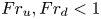 $Fr_u, Fr_d<1$), (ii) choked state (
 $Fr_u=Fr_{u,s}<1$,
  $Fr_d=Fr_{d,s}>1$) and (iii) supercritical state (
 $Fr_u\ (>Fr_{u,sc}), Fr_d>1$). An important feature of the regime diagram (figure 1a) is the presence of a band-gap in
  $Fr_u$ that separates the choked and supercritical states. The choked state and band-gap depend on the blocking ratio and obstacle geometry. The delta drag description incorporates both the action of drag and blocking at the same place, mimicking more closely processes that occur in a real flow, where the momentum flux and Froude number change simultaneously across the front and rear planes of the square cylinder.


4. Numerical results
4.1. Free-surface profile
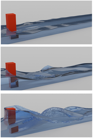
Figure 3 shows the free-surface elevation for  $Fr_0= 0.5$, 1.5 and 2.5. For a subcritical flow (
 $Fr_0 < 1$), the change in the water depth between upstream and downstream of the square cylinder is small, with the water flowing around its sides, and a series of standing waves is generated whose amplitude decreases downstream. For a choked flow (
 $Fr_0=1.5$), the upstream water height rises, and the downstream surface is characterised by a series of large oblique reflected waves. For a supercritical flow (
 $Fr_0 = 2.5$), the water begins to pile up around the front of the square cylinder, and a large rooster tail wake is created downstream. The results for figure 3(a,b) are consistent with the observations of Qi et al. (Reference Qi, Eames and Johnson2014), while figure 3(c) is consistent with Riviere et al. (Reference Riviere, Vouaillat, Launay and Mignot2017).

Figure 3. The free-surface flow for (a)  $Fr_0=0.5$, (b)
  $Fr_0=1.5$ and (c)
  $Fr_0=2.5$. The numerical results are visualised using Blender (www.blender.org).
Figure 4(a,b) show the variation of  $M$ and
  $Fr_l$ with distance along the channel. The momentum flux exhibits a finite decrease across the square cylinder as a consequence of the drag force (2.2) that acts on the obstruction, along with an associated jump in
  $Fr_l$, due to a change in the blocking ratio. The value of
  $M$ decreases across the upstream face of the obstruction and shows a partial recovery across the downstream face. The variation of
  $M$ with
  $Fr_l$ is shown in figure 4(c), where the paths upstream and downstream of the obstacle are colour coded; the choked state and band-gap are indicated.

Figure 4. Schematic of the channel, highlighting the three regions: upstream  $x/b<-1/2$ (red), drag region
  $|x|/b<1/2$ (black), and downstream
  $x/b>1/2$ (blue). The variation of (a)
  $M/M_0$ and (b)
  $Fr_l$ with position
  $x/b$ along the channel is shown for
  $Fr_0=0.2$, 0.4, 1.3, 1.9, 2.1 and 2.9. (c) The variation of
  $M/M_0$ with
  $Fr_l$, for contrasting values of
  $Fr_0$.
4.2. Flow state
Figure 5(a) shows a scatter plot of  $Fr_u$ and
  $Fr_d$ against
  $Fr_0$. The flow states are distinguished by
  $Fr_0$ and correspond to a subcritical state, a choked state where the flow transitions from subcritical to supercritical, and a supercritical state. The abrupt transition that occurs between the states is captured quite well by the numerical results, with the trend for
  $Fr_u$ collapsing onto the red curve. The 1-D model is based on local interaction and predicts the possibility of a hydraulic jump occurring in the range
  $|x|< b/2$ for the supercritical range; while the range is predicted, the 1-D model predicts a supercritical to critical transition that occurs within the span of the blocking–drag region and then a jump to a critical state as the flow expands. Since real flow transitions do not occur instantaneously but extend over several obstacle diameters, this unphysical transition is not observed in the numerical simulations. The numerical results show the supercritical state, and, indeed,
  $Fr_u$ is higher than anticipated from the 1-D model.

Figure 5. Comparison of the experimental (triangles, Qi et al. Reference Qi, Eames and Johnson2014), 1-D model (solid lines, Eames & Robinson Reference Eames and Robinson2022) and 3-D numerical simulation (circles) results. The subcritical, choked and supercritical states are indicated, along with the band-gap, in (a,b). In (a,c), red corresponds to upstream ( $Fr_u$) and black to downstream (
 $Fr_d$) values. (a) The influence of the initial Froude number (
 $Fr_0$) on the upstream and downstream Froude numbers. (b) The data in (a) replotted with
  $Fr_u$ versus
  $Fr_d$. (c,d) The variations of (upstream and downstream) water height and drag coefficient
  $C_{D0}$ against
  $Fr_0$, respectively.
Figure 5(b) shows a scatter plot of  $Fr_d$ versus
  $Fr_u$; for comparison, the experimental results of Qi et al. (Reference Qi, Eames and Johnson2014) are plotted, along with the 1-D results of Eames & Robinson (Reference Eames and Robinson2022). The 1-D model (red line) features a band-gap to the flow state, representing a span of
  $Fr_u$ where there is no steady state. Having repeated the Qi et al. (Reference Qi, Eames and Johnson2014) tests in a much longer flume, it has become apparent that the location of the flow transition, expressed generally by a hydraulic jump, moves further downstream as
  $Fr_0$ increases, meaning that while the flow transition conforms to an abrupt-change subcritical state and choked state, it appears to be continuous in the short flumes or short computational domains. The same comments apply to the transition from the choked state to the supercritical branch. The other challenge to being able to reproduce this discontinuity is simply that the bore speed decreases in magnitude, which means that the time taken to reach a steady state is much longer than the time for the drag forces to reach a steady state.
The 3-D numerical model captures the trend of the experimental results quite well. The absence of the flow regime case B2 described by Eames & Robinson (Reference Eames and Robinson2022) from the 3-D simulations is not surprising since its occurrence is based on the instantaneous adjustment from a supercritical to a subcritical state within the blocking–drag region. The critical states are due largely to the blocking and drag, and since the 1-D model uses an empirical closure for the drag force, the agreement with the 3-D simulations is good except at high  $Fr_0$. Here, the wake flow is a strongly 3-D flow.
4.3. Force on the square cylinder
In figure 5(d), the 3-D numerical results are compared against the 1-D model of Eames & Robinson (Reference Eames and Robinson2022) and the experimental results of Qi et al. (Reference Qi, Eames and Johnson2014). The forces are dominated by inertial effects, with viscous effects contributing less than 1 % to the total drag force. There are two main differences when compared with the 1-D model. First,  $C_{D0}$ is maximum at the choked state, which, while reflected in the experimental results (characterised by a degree of scatter), is not present in the 1-D model when the drag closure is based purely on a resistance. The limiting values of
  $C_{D0}$ determined numerically are slightly smaller than the experimental results, which, given the mesh independence study, suggests that the possible role of ambient turbulence (noted by Qi et al. Reference Qi, Eames and Johnson2014) may be important. The second difference is that the drag force for the supercritical flow state is much lower than that predicted by the 1-D model. Since the drag force can be expressed in terms of
  $Fr_u$ and
  $Fr_d$, this difference is attributed largely to a high
  $Fr_d$.
Figure 6(a) shows the variation of the drag coefficient  $C_D$ (based on the upstream flow conditions) with
  $Fr_u$ and confirms the amplification of
  $C_D$ at the choked state, corresponding to the maximum loss of the momentum flux. Of considerable interest is the drag coefficient in the supercritical regime, where
  $C_D\sim 1.3$. It is useful to distinguish between the drag coefficient corresponding to the force on the front (
 $C_{D1}$) and back (
 $C_{D2}$) of the cylinder (figure 6b). The pressure field has both a hydrostatic and a dynamic component. For subcritical flows, the separate drag coefficients increase with
  $Fr_u^{-2}$ since the force is dominated by a hydrostatic component with
  $C_{Di}\sim \tfrac{1}{2} gbh^2 / (\tfrac{1}{2} bhu^2) =1/Fr^2$; the inset of figure 6(b) confirms this trend. At the choked and supercritical state,
  $C_{D1}$ diminishes in magnitude and
  $C_{D2}$ tends to zero. For supercritical flows, we expect
  $F_D \sim \tfrac{1}{2} \rho g b h^2 = \tfrac{1}{2} \rho bh u^2$, giving
  $C_{D1}\sim 1$, which is close to the value 1.3. Figure 6(c) shows the variation of the instantaneous pressure field on the centreline of the cylinder, confirming a linear hydrostatic variation with
  $z$. For low
  $Fr$, the hydrostatic pressure dominates over the inertial component; while the pressure appears to be uniform across the region upstream of the square cylinder (the sides of the cylinder are identified), there is a small pressure reduction towards the edge of the front face as a consequence of the flow speeding up (figure 6d). Although the shape of the isobaric contours changes dramatically with
  $Fr_0$, the drag coefficient
  $C_D$ is normalised by the upstream flow properties, so its variation is less dramatic, taking the values
  $C_D = 2.67$,
  $3.15$ and
  $3.99$ for
  $Fr_0=0.1$,
  $0.5$ and
  $1.5$, respectively.

Figure 6. (a) The drag coefficient  $C_D$ is plotted as a function of
  $Fr_u$, and the results from the 3-D simulations are compared with experiments and the 1-D model. (b) The drag coefficients associated with the front and back of the cylinder (
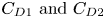 $C_{D1}\ {\rm and} \ C_{D2}$, respectively) are compared. The inset shows the results plotted on a larger range that corresponds to low
  $Fr_u$, with the lines corresponding to the prediction
  $C_{Di}\sim 1/Fr_u^2$. (c) The instantaneous pressure distribution on the upstream and downstream centreline of the cylinder. (d) The instantaneous pressure distribution over the whole cylinder surface is shown for
  $Fr_0=0.1$,
  $0.5$ and 1.5; the upstream and sides are indicated.
4.4. Influence of blocking ratio ( $0.1\le \phi _B \le 0.4$)

The blocking ratio caused by the cylinder has two dramatic effects on the flow: it tends to increase the flow speed at the side of the cylinder, forcing it to achieve a critical state at a lower  $Fr_u$, and it increases significantly the drag on the flow.
Figure 7(a) shows the variation of  $Fr_d$ with
  $Fr_u$ for different blocking ratios. Contrasting with Qi et al. (Reference Qi, Eames and Johnson2014), the new element is the supercritical flow regime and associated band-gap in
  $Fr_u$. More meaningful is the regime diagram figure 7(b) that distinguishes between different flow states, where the subcritical flow states are shown in red, the supercritical flow states in black, and the choked flow in blue. The blocking ratio greatly reduces the critical
  $Fr_u$ when the flow becomes choked, and increases the span across which the flow must jump from the choked state to the supercritical transition. The variation of the drag coefficient
  $C_D$ with
  $Fr_0$ is shown in figure 7(c). For low
  $Fr_0$, the influence of flow confinement on the drag coefficient is significant, even with small blocking ratios. However, for high
  $Fr_0$, the drag coefficient is weakly dependent on the blocking ratio because the bow shock tends to interact with the channel walls downstream of the cylinder.

Figure 7. (a) The influence of the blocking ratio  $\phi _B$ over the range
  $0.1\le \phi _B \le 0.4$ on the flow state and drag force. The
  $\times$ symbols represent the experimental results of Qi et al. (Reference Qi, Eames and Johnson2014). (b) Regime diagram showing the subcritical, choked and supercritical states determined from the 3-D calculations and the 1-D model of Eames & Robinson (Reference Eames and Robinson2022). (c) Variation of the drag coefficient
  $C_D$ with
  $Fr_0$ for different blocking ratios.
5. Conclusion
The free-surface channel flow past a rigid body displays a remarkable degree of complexity, as characterised by the different flow states. A new detailed analysis of the flow states has been presented over a range of  $Fr_0$ spanning subcritical, choked and supercritical states. The computational analysis has confirmed the presence of a range of
  $Fr_u$ where a steady solution is not present and given insight into the supercritical branch, which was unstudied previously.
There is some initial indication by Eames & Robinson (Reference Eames and Robinson2022) that the free-surface channel flows past an obstruction (formed, for instance, by a dam-break release) locks on to a locus of points that follows the  $Fr_u$–
 $Fr_d$ trajectory (shown in figure 3b) linking the supercritical state to the choked state. This underlines the significance of the present study in validating the presence of the multiple flow states and their use in characterising the types of flows that can occur.
Acknowledgements
Support from UCL through the use of Myriad and Kathleen is gratefully acknowledged.
Funding
Thanks to H.R. Wallingford Group Ltd for administering award 166164 on Computational Tools for Assessing Building Vulnerability from Tsunamis.
Declaration of interests
The authors report no conflict of interest.


 Open access