


1. Introduction
The dynamic wetting behaviour of liquid droplets on soft solid substrates has received a great deal of attention lately, due to its relevance in diverse applications (Bico, Reyssat & Roman Reference Bico, Reyssat and Roman2018) ranging from biology, i.e. the inhibition of the dispersal of cancer cells (Douezan, Dumond & Brochard-Wyart Reference Douezan, Dumond and Brochard-Wyart2012) or the control of medicine dispersal on tissues, to the control of the spreading of the deposited particles over a compliant substrate after the evaporation of ink-jetted microdroplets (Park & Moon Reference Park and Moon2006) and microfabrication of materials in technology (Bonaccurso et al. Reference Bonaccurso, Butt, Hankeln, Niesenhaus and Graf2005; Pericet-Camara et al. Reference Pericet-Camara, Best, Nett, Gutmann and Bonaccurso2007; Kong et al. Reference Kong, Tamargo, Kim, Johnson, Gupta, Koh, Chin, Steingart, Rand and McAlpine2014).
The evaporation of droplets on rigid substrates has been widely studied over the years, underlining various aspects of evaporation such as droplet lifetimes (Stauber et al. Reference Stauber, Wilson, Duffy and Sefiane2014, Reference Stauber, Wilson, Duffy and Sefiane2015), the impact of capillary flow on the coffee stain effect (Deegan et al. Reference Deegan, Bakajin, Dupont, Huber, Nagel and Witten1997) or the effect of substrate properties (Erbil Reference Erbil2012). A key concept in droplet evaporation is the so-called shielding effect, where neighbouring droplets interact with each other, since the presence of the vapour from adjacent droplets reduces the evaporation rate and increases the droplet lifetime in comparison with those of a single isolated droplet (Fabrikant Reference Fabrikant1985; Wray, Duffy & Wilson Reference Wray, Duffy and Wilson2020; Masoud, Howell & Stone Reference Masoud, Howell and Stone2021; Wray et al. Reference Wray, Wray, Duffy and Wilson2021). On the contrary, the study of droplet evaporation on compliant solid substrates is not very substantial so far.
The unbalanced vertical forces acting on the contact line of the liquid result in a local deformation of the compliant substrate affecting droplet shape and, ultimately, the dynamics of the flow (Andreotti & Snoeijer Reference Andreotti and Snoeijer2020). This unique attribute of the compliant substrates is responsible for the creation of a macroscopic surface protrusion, most widely referred to as a wetting ridge (Shanahan Reference Shanahan1988; Park et al. Reference Park, Weon, Lee, Lee, Kim and Je2014; Chen et al. Reference Chen, Askounis, Koutsos, Valluri, Takata, Wilson and Sefiane2020). The structure of the wetting ridge is an immediate outcome of the balance between capillary and elastic forces, while a key role of the solid surface tension has been recently identified (Jerison et al. Reference Jerison, Xu, Wilen and Dufresne2011; Marchand et al. Reference Marchand, Das, Snoeijer and Andreotti2012; Style & Dufresne Reference Style and Dufresne2012; Style et al. Reference Style, Che, Wettlaufer, Wilen and Dufresne2013). Besides slowing down the contact line, the wetting ridge can also constitute the reason for periodic stick–slip behaviour, with a periodic depinning of the contact line (Kajiya et al. Reference Kajiya, Daerr, Narita, Royon, Lequeux and Limat2012, Reference Kajiya, Brunet, Royon, Daerr, Receveur and Limat2014; Lopes & Bonaccurso Reference Lopes and Bonaccurso2013; Yu, Wang & Zhao Reference Yu, Wang and Zhao2013; Karpitschka et al. Reference Karpitschka, Pandey, Lubbers, Weijs, Botto, Das, Andreotti and Snoeijer2016; van Gorcum et al. Reference van Gorcum, Andreotti, Snoeijer and Karpitschka2018; Mokbel, Aland & Karpitschka Reference Mokbel, Aland and Karpitschka2022). Starting from a rigid substrate, when we increase the substrate softness we observe an initial strong increase in the wetting ridge size while the droplet footprint is kept relatively constant, which is replaced by a strong depression of the substrate under the droplet in much softer substrates (Charitatos & Kumar Reference Charitatos and Kumar2020; Henkel, Snoeijer & Thiele Reference Henkel, Snoeijer and Thiele2021). The arising solid angle is governed by a balance of surface tensions (Marchand et al. Reference Marchand, Das, Snoeijer and Andreotti2012; Style & Dufresne Reference Style and Dufresne2012; Style et al. Reference Style, Che, Wettlaufer, Wilen and Dufresne2013). The possible strain dependence of the solid surface tension (i.e. the Shuttleworth effect) (Andreotti & Snoeijer Reference Andreotti and Snoeijer2016; Xu et al. Reference Xu, Jensen, Boltyanskiy, Sarfati, Style and Dufresne2017; Pandey et al. Reference Pandey, Andreotti, Karpitschka, van Zwieten, van Brummelen and Snoeijer2020; Henkel et al. Reference Henkel, Essink, Hoang, van Zwieten, van Brummelen, Thiele and Snoeijer2022) gives rise to another complexity.
Depending on a combination of capillarity and bulk elasticity, adjacent droplets on solid substrates can interact, leading either to droplet attraction and even coalescence on thick substrates, or to droplet repulsion on thinner substrates (Hernández-Sánchez et al. Reference Hernández-Sánchez, Lubbers, Eddi and Snoeijer2012; Karpitschka et al. Reference Karpitschka, Pandey, Lubbers, Weijs, Botto, Das, Andreotti and Snoeijer2016; Leong & Le Reference Leong and Le2020). Karpitschka et al. (Reference Karpitschka, Pandey, Lubbers, Weijs, Botto, Das, Andreotti and Snoeijer2016) described the droplet interaction when deposited on soft solids as the ‘inverse Cheerios effect’ with direct reference to the liquid-on-solid analogue of the so-called ‘Cheerios effect’ (Vella & Mahadevan Reference Vella and Mahadevan2005); the latter refers to solid particles’ attraction when floating on liquids, mediated by surface tension forces, and it has been named after the sticking of breakfast cereals either to the walls of a bowl or to each other. However, there are substantial differences between the ‘Cheerios effect’ and the ‘inverted Cheerios effect’ regarding the driving force and the mechanism which mediates the interaction. The shape of the liquid interface in the ‘Cheerios effect’ is specified by the balance between surface tension and gravity, while the interaction is driven by a change in gravitational potential energy. On the contrary, in the ‘inverse Cheerios effect’ there is no gravity involved and the shape of the solid interface is specified by elastocapillarity (Karpitschka et al. Reference Karpitschka, Das, van Gorcum, Perrin, Andreotti and Snoeijer2015).
Despite the innumerable studies concerning droplet coalescence (Eggers, Lister & Stone Reference Eggers, Lister and Stone1999; Aarts et al. Reference Aarts, Lekkerkerker, Guo, Wegdam and Bonn2005), not many of them consider the role that a compliant substrate might play in the process. More recently, Henkel et al. (Reference Henkel, Snoeijer and Thiele2021) investigated the two basic coarsening modes of two droplets on soft substrates without evaporation; the volume or mass transfer mode (also referred to as drop collapse mode, diffusion-controlled ripening or Ostwald ripening) and the translation mode (also referred to as coalescence, collision or migration mode). On the one hand, in the mass transfer mode, material is transferred from the small drop to the larger one until the smaller drop has completely vanished, while the centres of mass of each droplet remain constant. This mass transfer might occur either through the vapour phase in case of volatile droplets, or through an adsorption layer in case of non-evaporating partially wetting fluids. On the other hand, in the translation mode, there is droplet migration towards each other, until their contact lines touch, leading to coalescence (Henkel et al. Reference Henkel, Snoeijer and Thiele2021).
When compared with rigid substrates, early experimental studies (Lopes & Bonaccurso Reference Lopes and Bonaccurso2012; Pu & Severtson Reference Pu and Severtson2012; Lopes & Bonaccurso Reference Lopes and Bonaccurso2013; Yu et al. Reference Yu, Wang and Zhao2013; Chuang et al. Reference Chuang, Chu, Lin and Chen2014; Gerber et al. Reference Gerber, Lendenmann, Eghlidi, Schutzius and Poulikakos2019) highlighted the faster evaporation of droplets observed on softer substrates, due to the longer pinning of the contact line throughout evaporation, caused by the formation of the wetting ridge. In addition, some of these experimental studies (Lopes & Bonaccurso Reference Lopes and Bonaccurso2013; Yu et al. Reference Yu, Wang and Zhao2013) revealed that while in the initial stages of evaporation, the droplet appears to remain pinned, while the contact angle is decreased. After the droplet depins, the opposite behaviour is observed, i.e. the contact angle remains constant and the contact radius decreases. Then, at the late stages of droplet evaporation, the contact angle slightly increases, before ultimately decrease until the droplet completely evaporates.
As it has been established in studies for rigid substrates, the dynamics of the contact line plays a crucial role on droplet evaporation (Lopes & Bonaccurso Reference Lopes and Bonaccurso2012, Reference Lopes and Bonaccurso2013; Pu & Severtson Reference Pu and Severtson2012; Yu et al. Reference Yu, Wang and Zhao2013; Chuang et al. Reference Chuang, Chu, Lin and Chen2014; Gerber et al. Reference Gerber, Lendenmann, Eghlidi, Schutzius and Poulikakos2019) and in order to model the contact line motion an approach, followed by several researchers, has been to introduce the effect of disjoining pressure, by assuming the presence of an adsorbed precursor film ahead of the droplet, which is stabilised by the action of intermolecular interactions between the two interfaces. The presence of the precursor film is evident in experimental studies with microscopic techniques (Kavehpour, Ovryn & McKinley Reference Kavehpour, Ovryn and McKinley2003; Xu et al. Reference Xu, Shirvanyants, Beers, Matyjaszewski, Rubinstein and Sheiko2004; Hoang & Kavehpour Reference Hoang and Kavehpour2011) and constitutes the reason for the levelled transition from the contact line to the flat gas–solid interface, circumventing the singularity arising from the shear stress (Wang et al. Reference Wang, Karapetsas, Valluri, Sefiane, Williams and Takata2021), due to the contradiction between the non-zero displacement on the contact line and the no-slip boundary condition on the liquid–solid interface on the same point. This approach has been widely implemented for the modelling of not only perfectly wetting fluids (Bonn et al. Reference Bonn, Eggers, Indekeu, Meunier and Rolley2009), but also partially wetting fluids (Schwartz Reference Schwartz1998; Schwartz & Eley Reference Schwartz and Eley1998; Gomba & Homsy Reference Gomba and Homsy2010). A similar approach has been also used by Charitatos & Kumar (Reference Charitatos and Kumar2021) to examine droplet evaporation on partially wetted soft viscoelastic substrates.
To account for the droplet evaporation, two approximations have been mostly used (Wilson & D'Ambrosio Reference Wilson and D'Ambrosio2023). In the so-called one-sided model, the attention is solely drawn to the liquid phase, since vapour viscosity, density and thermal conductivity are considered negligible. In this approach, evaporation is limited by the rate on which the molecules of the solvent are headed from the liquid towards the gas phase (Burelbach, Bankoff & Davis Reference Burelbach, Bankoff and Davis1988). On that principle, the work of Moosman & Homsy (Reference Moosman and Homsy1980), Ajaev & Homsy (Reference Ajaev and Homsy2001) and later Ajaev (Reference Ajaev2005) considered an adsorbed thin film ahead of the evaporating liquid, with non-zero film thickness, which is in thermodynamic equilibrium with both the solid and the gas phases. The work of Ajaev has been the grounding principle for many researchers studying, qualitatively, droplet spreading and evaporation of more complex systems, such as droplets with nanoparticles (Matar, Craster & Sefiane Reference Matar, Craster and Sefiane2007), the deposition of particles while in the presence of surfactants (Karapetsas, Sahu & Matar Reference Karapetsas, Sahu and Matar2016), as well as the evaporation of droplets which consist of ethanol–water or other binary mixtures (Williams et al. Reference Williams, Karapetsas, Mamalis, Sefiane, Matar and Valluri2021), or the vapour adsorption of hygroscopic aqueous solution droplets (Wang et al. Reference Wang, Karapetsas, Valluri, Sefiane, Williams and Takata2021). Concerning droplet evaporation on compliant substrates, the only theoretical work so far is the work of Charitatos & Kumar (Reference Charitatos and Kumar2021), where a one-sided model is developed to study the evaporation of a single droplet.
However, when the evaporation is diffusion-limited and, hence, the vapour phase cannot be considered irrelevant, quantitative results can only be achieved by employing a two-sided approximation (Sultan, Boudaoud & Amar Reference Sultan, Boudaoud and Amar2005; Schofield et al. Reference Schofield, Wray, Pritchard, Wilson and Sefiane2020; Wray et al. Reference Wray, Duffy and Wilson2020). Typically, one-sided models consider that the evaporation flux is only a function of pressure and temperature differences in the liquid–gas interface and the transport equations in the liquid phase are the only prerequisite for the system modelling. On the contrary, the diffusion-limited model includes the simultaneous solution of a diffusion equation concerning the vapour gas phase concentration. The second approach entails a higher computational cost but provides a more accurate description of phase change phenomena (Deegan et al. Reference Deegan, Bakajin, Dupont, Huber, Nagel and Witten1997; Hu & Larson Reference Hu and Larson2005; Masoud & Felske Reference Masoud and Felske2009; Cazabat & Guéna Reference Cazabat and Guéna2010; Mikishev & Nepomnyashchy Reference Mikishev and Nepomnyashchy2013; Larson Reference Larson2014). A common assumption to reduce the computational cost, is to consider that the droplet retains a spherical-cap shape. This assumption, though, is not always safe, since the droplet shape might be significantly distorted by forces, such as gravitational forces (e.g. evaporation on inclined substrates), the effect of Marangoni or elastic stresses, etc. Hartmann et al. (Reference Hartmann, Diddens, Jalaa and Thiele2023) recently developed a long-wave model of a sessile shallow droplet of evaporating partially wetting fluid on a rigid substrate, which, similarly to the earlier work of Sultan et al. (Reference Sultan, Boudaoud and Amar2005), captured the transition between the diffusion-limited and the one-sided model.
Several authors have also investigated the effect of Marangoni stresses on droplet spreading and evaporation. Marangoni flows can be induced by thermal gradients, a variation in the concentration of surfactants, or by the presence of binary mixtures (Dunn et al. Reference Dunn, Duffy, Wilson and Holland2009a; Wang et al. Reference Wang, Karapetsas, Valluri, Sefiane, Williams and Takata2021; Williams et al. Reference Williams, Karapetsas, Mamalis, Sefiane, Matar and Valluri2021). The coffee-ring effect may be suppressed by the action of Marangoni stresses (Karapetsas et al. Reference Karapetsas, Sahu and Matar2016; Seo et al. Reference Seo, Yang, Chae and Shin2017), since they counter the outward liquid flow facilitated by contact-line pinning. Additionally, the coalescence of merging droplets with different surface tensions (such as water and ethanol) has been shown to be strongly delayed (Karpitschka & Riegler Reference Karpitschka and Riegler2010; Chen et al. Reference Chen, Gao, Xia, Li, Liu and Ding2021). Concerning evaporating droplets, Talbot et al. (Reference Talbot, Berson, Brown and Bain2012), Schofield et al. (Reference Schofield, Wilson, Pritchard and Sefiane2018) and Dunn et al. (Reference Dunn, Wilson, Duffy, David and Sefiane2009b) showed that the thermal effects can significantly extend the droplet lifetime.
There have been different approaches in the literature to describe soft substrate wetting, ranging from the development of long-wave models (Kumar & Matar Reference Kumar and Matar2004; Matar, Gkanis & Kumar Reference Matar, Gkanis and Kumar2005; Gielok et al. Reference Gielok, Lopes, Bonaccurso and Gambaryan-Roisman2017; Gomez & Velay-Lizancos Reference Gomez and Velay-Lizancos2020) to full-scale computational studies (Bueno et al. Reference Bueno, Bazilevs, Juanes and Gomez2017, Reference Bueno, Bazilevs, Juanes and Gomez2018). Kumar & Matar (Reference Kumar and Matar2004) and Matar et al. (Reference Matar, Gkanis and Kumar2005) first developed a long-wave approach to study the nonlinear evolution of thin liquid films dewetting near soft elastomeric layers. Charitatos & Kumar (Reference Charitatos and Kumar2020) followed Matar's work for droplet spreading on soft solid substrates, while Charitatos & Kumar (Reference Charitatos and Kumar2021), extended their own work developing a one-sided model to examine droplet evaporation on viscoelastic substrates.
Building on the latter model, the present paper presents a detailed and comprehensive theoretical model for the investigation of the dynamics of a system of two evaporating droplets residing on a compliant solid substrate. The droplets may interact through the developed elastic stresses in the viscoelastic substrate which is modelled using the Kelvin–Voigt model. When the droplets are exposed to the atmosphere, a further question is raised, concerning the effect of the local variations in vapour concentration on the evaporation rate of the droplets. To this end, we develop a two-sided evaporation model following a similar approach with earlier studies for rigid substrates (Sultan et al. Reference Sultan, Boudaoud and Amar2005; Doumenc & Guerrier Reference Doumenc and Guerrier2011). Thus, apart from the viscoelastic substrate, our model unravels the potential of communication of the droplets through the atmosphere, while also taking fully into consideration the effects of evaporative cooling and induced thermocapillary phenomena. To remove the stress singularity that arises at the moving contact line, we assume the presence of a sufficiently thin precursor film. The precursor film is stabilised and evaporation therein is suppressed through the inclusion of a disjoining pressure.
The rest of the paper is organised as follows. The problem is formulated in § 2 and the equations governing the flow dynamics are discussed. The scaling and resulting evolution equations are presented in §§ 3 and 4, respectively. Results are presented and discussed in § 5, followed by concluding remarks in § 6.
2. Problem statement and model formulation
2.1. Description of the problem
We consider the behaviour of a single droplet or a system of two two-dimensional sessile evaporating droplets, with initial cross-sectional area  $\hat {V}$, placed on an incompressible linear viscoelastic solid substrate, which is also referred to as soft substrate. At
  $\hat {t}=0$, the droplet is resting on the soft substrate and has an initial footprint half-width
  $\hat {l}_0$ and an initial height
  $\hat {h}_0$ (figure 1a). The liquid–solid interface is originally located at
  $\hat {z}=0$. The soft substrate is originally undistorted and attached to a rigid substrate at
  $\hat {z}=-\hat {H}$; the rigid substrate is highly conductive with constant temperature
  $\hat {T}_b$. The soft substrate is characterised by density
  $\hat {\rho }_s$, viscosity
  $\hat {\eta }_s$, thermal conductivity
  $\hat {\lambda }_w$, shear modulus
  $\hat {E}$ and constant liquid–solid interfacial tension
  $\hat {\gamma }$, which is independent of strain; the presence of an immiscible liquid solvent in the soft substrate is assumed. The droplet is assumed to have constant density
  $\hat {\rho }_l$, viscosity
  $\hat {\eta }_l$, thermal conductivity
  $\hat {\lambda }$, specific heat capacity
  $\hat {c}_p$ and saturation temperature
  $\hat {T}_{sat}$. The liquid–gas interfacial tension,
  $\hat {\sigma }$, is assumed to be a linear function of temperature:
 \begin{equation} \hat{\sigma} = \hat{\sigma}_0 - \frac{\partial \hat{\sigma}}{\partial \hat T}(\hat{T}_s - \hat{T}_{ref}), \end{equation}
where  $\hat {\sigma }_0$ is the surface tension at the reference temperature
  $\hat {T}_{ref}$, and
  $\hat {T}_s$ is the local temperature at the liquid–gas interface. The reference temperature was considered to be equal to the bulk temperature of the gas
  $\hat {T}_{b}$.

Figure 1. Schematic diagram of model geometry. (a) Initial configuration of a droplet with initial half-width  $\hat {l}_0$ and initial height
  $\hat {h}_0$ resting on an undeformed compliant substrate at
  $\hat {z}=0$, which is attached to a rigid substrate at
  $\hat {z}=-\hat {H}$. (b) The soft solid deforms while the system of two droplets spreads and evaporates. (c) Magnified view of the contact line, where
  $\hat {\beta }$ is the precursor film thickness,
  $\hat {\theta }$ is the apparent contact angle and
  $\hat {\xi }_{max}$ denotes the maximum height of the wetting ridge. The local thickness of each droplet is given by
  $\hat {h}(\hat {x},\hat {t})=\hat {\zeta }(\hat {x},\hat {t})-\hat {\xi }(\hat {x},\hat {t})$.
At  $\hat {t}>0$, the droplet, being in an unsaturated environment, evaporates causing the deformation of the soft solid substrate. The liquid–solid interface is located at
  $\hat {z}=\hat {\xi }(\hat {x},\hat {t})$, with an outward normal unit vector of
  $\hat {\boldsymbol{n}}_s=(-{\partial \hat {\xi }}/{\partial \hat {x}},1) / \sqrt {1+({\partial \hat {\xi }}/{\partial \hat {x}})^2}$ while the liquid–air interface is located at
  $\hat {z}=\hat {\zeta }(\hat {x},\hat {t})$, with an outward normal unit vector of
  $\hat {\boldsymbol{n}}_l=(-{\partial \hat {\zeta }}/{\partial \hat {x}},1) / \sqrt {1+({\partial \hat {\zeta }}/{\partial \hat {x}})^2}$. The tangential unit vectors are
  $\hat {\boldsymbol{t}}_s=(1, {\partial \hat {\xi }}/{\partial \hat {x}}) / \sqrt {1+({\partial \hat {\xi }}/{\partial \hat {x}})^2}$ and
  $\hat {\boldsymbol{t}}_l=(1, {\partial \hat {\zeta }}/{\partial \hat {x}}) / \sqrt {1+({\partial \hat {\zeta }}/{\partial \hat {x}})^2}$ for the liquid–solid and the liquid–air interface, respectively.
We assume that the droplet is released into a thin precursor film; evaporation in the film is stabilised by the disjoining pressure which accounts for intermolecular van der Waals interactions. The inclusion of the precursor film removes the stress singularity that can arise at the moving contact line (see figure 1c). This approach also allows us to easily account for the evaporation of multiple droplets as well as their interactions; in figure 1(b) we depict a system of two evaporating droplets, of the same initial radius and height. Ahead of the contact line the dimensional precursor film thickness is denoted with  $\hat {\beta }$ (see figure 1c) and the apparent contact angle is
  $\hat {\theta }$. Concerning the wetting ridge, its maximum height is denoted as
  $\hat {\xi }_{max}$. Moreover, the length of each droplet, that is the distance between the two contact lines, is denoted as
  $\Delta \hat {x}_{cl}$, while the length of the computational domain is denoted as
  $\hat{L}_x$ (i.e.
  $0<\hat {x}<\hat {L}_x$). In this domain, the global centre of mass of the system is located at
  $\hat {x}=\hat {x}_{cm,g}$ and the centre of mass of each droplet is located at
  $\hat {x}=\hat {x}_{cm,l}$ and
  $\hat {x}=\hat {x}_{cm,r}$, respectively. Consequently, the distance between the two centres of mass is denoted as
  $\Delta \hat {x}_{cm}=\hat {x}_{cm,r}-\hat {x}_{cm,l}$. The presented model geometry in figure 1 constitutes the reference layout for the rest of this paper.
In the present work, the droplets are assumed to be so thin that the droplet aspect ratio  $\mathbf {\epsilon }=\hat {h}_0/\hat {R}_0$ is considered to be much smaller than unity;
  $\hat {R}_0$ is a characteristic length scale, defined as
  $\hat {R}_0=2\hat {l}_0/3$. Under this assumption, we will employ the lubrication approximation to derive a reduced set of governing evolution equations. Furthermore, gravitational forces are neglected, since the solid and liquid Bond numbers
  $Bo_s=\hat {\rho }_s\hat {g}\hat {R}_0^2/\hat {\sigma }$ and
  $Bo_l=\hat {\rho }_l\hat {g}\hat {R}_0^2/\hat {\sigma }$ are assumed to be less than unity; this condition typically holds for small droplets. A two-dimensional Cartesian coordinate system
  $(\hat {x},\hat {z})$ is used to model the velocity field, which is described by a function of
  $\hat {\boldsymbol {v}}=(\hat {v}_x, \hat {v}_z)$, whereas the solid displacement is given by
  $\hat {\boldsymbol {u}}=(\hat {u}_x, \hat {u}_z)$. Our model can describe a typical system of water droplets drying on polydimethylsiloxane (PDMS) substrates and the physical properties of such a system are given in table 1.
Table 1. Properties of water and PDMS at 20  $^\circ$C and 1 atm.

2.2. Liquid phase
The mass, momentum and energy conservation equations for the liquid are given by
 \begin{gather} \hat{\boldsymbol{\nabla}} \boldsymbol{\cdot} \hat{\boldsymbol{v}} = 0, \end{gather}
 \begin{gather}\hat{\rho}_l \left( \frac{\partial \hat{\boldsymbol{v}}}{\partial \hat{t}} + \hat{\boldsymbol{v}} \boldsymbol{\cdot} \hat{\boldsymbol{\nabla}} \hat{\boldsymbol{v}} \right) ={-} \hat{\boldsymbol{\nabla}} \hat{p}_l + \hat{\eta}_l \hat{\nabla}^2 \hat{\boldsymbol{v}}, \end{gather}
 \begin{gather}\frac{\partial \hat{T}}{\partial \hat{t}} + \hat{\boldsymbol{v}} \boldsymbol{\cdot} \hat{\boldsymbol{\nabla}} \hat{T} - \hat{\alpha}_l \hat{\nabla}^2 \hat{T} = 0, \end{gather}
where  $\hat {p}_l$ is the liquid pressure,
  $\hat {\boldsymbol {\nabla }}=(\partial _{\hat {x}},\partial _{\hat {y}})$ is the gradient operator,
  $\hat {T}$ is the temperature and
  $\hat {\alpha }_l={\hat {\lambda }}/{(\hat {\rho }_l \hat {c}_p)}$ is the thermal diffusivity of the liquid. Along the free interface
  $\hat {z}=\hat {\zeta }(\hat {x},\hat {t})$, the liquid velocity
  $\hat {\boldsymbol {v}}=(\hat {v}_x, \hat {v}_z)$ differs from the velocity of the interface
  $\hat {\boldsymbol {v}}_{\boldsymbol {s}}=(\hat {v}_{xs}, \hat {v}_{zs})$. If the evaporative flux is denoted by
  $\hat {J}$, then
 \begin{equation} \hat{J}=\hat{\rho}_l (\hat{\boldsymbol{v}}-\hat{\boldsymbol{v}}_{\boldsymbol{s}}) \boldsymbol{\cdot} \hat{\boldsymbol{n}}_{\boldsymbol{l}}. \end{equation}
Furthermore, along the free interface, the local mass, energy and force balances are given by
 \begin{gather} \hat{J}=\hat{\rho}_l (\hat{\boldsymbol{v}}-\hat{\boldsymbol{v}}_{\boldsymbol{s}}) \boldsymbol{\cdot} \hat{\boldsymbol{n}}_l=\hat{\rho}_g (\hat{\boldsymbol{v}}_{\boldsymbol{g}}-\hat{\boldsymbol{v}}_{\boldsymbol{s}}) \boldsymbol{\cdot} \hat{\boldsymbol{n}}_{\boldsymbol{l}}, \end{gather}
 \begin{gather}\hat{J} \hat{L}_v + \hat{\lambda} \hat{\boldsymbol{\nabla}} \hat{T} \boldsymbol{\cdot} \hat{\boldsymbol{n}}_{\boldsymbol{l}} - \hat{\lambda}_g \hat{\boldsymbol{\nabla}} \hat{T}_g \boldsymbol{\cdot} \hat{\boldsymbol{n}}_{\boldsymbol{l}}=0, \end{gather}
 \begin{gather}\hat{J} (\hat{\boldsymbol{v}} - \hat{\boldsymbol{v}}_{\boldsymbol{g}}) - \hat{\boldsymbol{n}}_{\boldsymbol{l}} \boldsymbol{\cdot} (-\hat{p}_l \boldsymbol{\mathsf{I}} +\hat{\eta}_l (\hat{\boldsymbol{\nabla}} \hat{\boldsymbol{v}} +(\hat{\boldsymbol{\nabla}} \hat{\boldsymbol{v}})^{\rm T}) -\hat{p}_g \hat{\boldsymbol{n}}_{\boldsymbol{l}}+ \hat{\varPi} \hat{\boldsymbol{n}}_{\boldsymbol{l}}+ 2\hat{\kappa}_l \hat{\sigma} \hat{\boldsymbol{n}}_{\boldsymbol{l}} +\hat{\boldsymbol{\nabla}}_s \hat{\sigma} = 0, \end{gather}
where  $\hat {\rho }_g$,
  $\hat {\lambda }_g$,
  $\hat {\boldsymbol {v}}_{\boldsymbol {g}}$ and
  $\hat {T}_g$ denote the density, the thermal conductivity, the velocity and the temperature of the gas phase, respectively. Here
  $\hat {L}_v$ is the specific latent internal heat of vaporisation,
  $\boldsymbol{\mathsf{I}}$ is the identity tensor,
  $\hat {\kappa }_l$ is the mean curvature of the free interface, while
  $\hat {\boldsymbol {\nabla }}_s$ is the surface gradient operator. In the above equations,
  $\hat {\kappa }_l=\hat {\boldsymbol {\nabla }}_s \boldsymbol{\cdot} \hat {\boldsymbol {n}}_{\boldsymbol {l}}$ and
  $\hat {\boldsymbol {\nabla }}_s=(I-\hat {\boldsymbol {n}}_{\boldsymbol {l}} \hat {\boldsymbol {n}}_{\boldsymbol {l}}) \boldsymbol{\cdot} \hat {\boldsymbol {\nabla }}$. Finally,
  $\hat {\varPi }$ stands for the disjoining pressure, which, taking into consideration the van der Waals interaction, is equal to
 \begin{equation} \hat{\varPi}=\hat{A}_1 \left[\left(\frac{\hat{A}_2}{\hat{h}}\right)^n - \left(\frac{\hat{A}_2}{\hat{h}}\right)^c \right], \end{equation}
where  $\hat {A}_1=\hat {A}_{Ham}/\hat {A}_2^3$, is a constant that describes the intermolecular interactions between the liquid–gas and the liquid–solid interfaces,
  $\hat {A}_{Ham}$ the Hamaker constant,
  $\hat {A}_2$ is a constant of the same order of magnitude as the precursor film thickness
  $\hat {\beta }$.
  $\hat {h}$ denotes the droplet thickness and
  $n>c>1$. Moreover, the kinematic boundary condition along the moving interface
  $\hat {z}=\hat {\zeta }(\hat {x},\hat {t})$, is described as
 \begin{equation} \frac{\partial \hat{\zeta}}{\partial \hat{t}} + \hat{v}_{xs} \frac{\partial \hat{\zeta}}{\partial \hat{x}}= \hat{v}_{zs}. \end{equation}
2.3. Gas phase
The gas phase is assumed to comprise air and vapour, but it is not saturated by vapour. Typically, we may consider that  $\varLambda _g={\hat {\lambda }}/{\hat {\lambda }_g}\ll 1$, and under this assumption the bulk temperature of the gas can be assumed to be constant and equal to
  $\hat {T}_b$. Moreover, we assume that the viscosity of the gas,
  $\hat {\eta }_g$, is much smaller than the viscosity of the liquid phase, i.e.
  $\hat {\eta }_g/\hat {\eta }_l \ll 1$ and therefore the gas can be considered as inviscid and passive with respect to the fluid.
The droplet evaporation is approached using the generalised diffusion-limited model developed by Sultan et al. (Reference Sultan, Boudaoud and Amar2005), in which evaporation is considered limited by the solvent vapour diffusion in the air; this model is able to capture the transition between the diffusion-limited and the one-sided model. The vapour concentration  $\hat {\rho }^v$ in the gas phase is described by the Laplace's equation, due to the fact that the gas phase is considered to be at rest and the characteristic evaporation time is much larger than the respectivediffusion time. As a result, we get
 \begin{equation} \hat{\nabla}^2 \hat{\rho}^v=0. \end{equation}
The vapour mass flux  $\hat {J}$ is assumed to be limited by the rate of diffusion and thus
 \begin{equation} \hat{J}={-}\mathcal{\hat{D}}_v(\hat{\boldsymbol{n}}_{\boldsymbol{l}} \boldsymbol{\cdot} \hat{\boldsymbol{\nabla}} \hat{\rho}^v)|_{\hat{\zeta}}, \end{equation}
where  $\mathcal {\hat {D}}_v$ the diffusion vapour coefficient. Considering also that the vapour mass flux
  $\hat {J}$ is proportional to the departure from equilibrium at the liquid–gas interface (Schrage Reference Schrage1953; Plesset & Prosperetti Reference Plesset and Prosperetti1976; Moosman & Homsy Reference Moosman and Homsy1980), the following linear constitutive equation, most commonly known as the Hertz–Knudsen equation, for
  $\hat {J}$ can be used:
 \begin{equation} \hat{J}=\alpha \left(\frac{\hat{R} \hat{T}_{s}}{2{\rm \pi} \hat{M}}\right)^{{1}/{2}} (\hat{\rho}^{ve}-\hat{\rho}^v|_{\hat{\zeta}}), \end{equation}
where  $\alpha$ is the accommodation coefficient, usually considered equal to unity near equilibrium. Here
  $\hat {R}$ denotes the universal gas constant,
  $\hat {T}_{s}$ denotes the temperature of the liquid–gas interface,
  $\hat {\rho }^v$ is the local vapour concentration in the gas phase and
  $\hat {\rho }^{ve}$ is the equilibrium vapour concentration.
In order to get a boundary condition for the vapour concentration  $\hat {\rho }^v$ at
  $\hat {z}=\hat {\zeta }$, we can combine (2.12) and (2.13), which leads to
 \begin{equation} -\mathcal{\hat{D}}_v(\hat{\boldsymbol{n}}_{\boldsymbol{l}} \boldsymbol{\cdot} \hat{\boldsymbol{\nabla}} \hat{\rho}^v)|_{\hat{\zeta}}=\alpha \left(\frac{\hat{R} \hat{T}_{s}}{2{\rm \pi} \hat{M}}\right)^{{1}/{2}} (\hat{\rho}^{ve}-\hat{\rho}^v|_{\hat{\zeta}}). \end{equation}
Finally, following a similar procedure as described by (Moosman & Homsy Reference Moosman and Homsy1980), the following equation for the equilibrium vapour concentration can be derived:
 \begin{equation} \hat{\rho}^{ve}=\hat{\rho}^v_{ref}+\frac{\hat{M} \hat{\rho}^v_{ref}}{\hat{\rho}_l \hat{R} \hat{T}_{ref}}({-}2\hat{H}_l \hat{\sigma} -\hat{\varPi})+\frac{\hat{L}_v \hat{M} \hat{\rho}^v_{ref}}{\hat{R} \hat{T}^2_{ref}}(\hat{T}_s-\hat{T}_{ref}), \end{equation}
where  $\hat {\rho }^v_{ref}$ is the equilibrium vapour concentration at the reference temperature.
At the far-field boundary, the most natural choice would be to impose a constant vapour concentration at infinity. However, since it is known that for the diffusion-limited model there is no analytical solution in two-dimensional half-space (Schofield et al. Reference Schofield, Wray, Pritchard, Wilson and Sefiane2020), we follow a similar approach to Schofield et al. (Reference Schofield, Wray, Pritchard, Wilson and Sefiane2020) considering a finite domain of the gas phase and the far-field condition is replaced by a similar Dirichlet condition at a distant, but finite, boundary. Thus, far from the droplet ( $\hat {z}=\hat {d}_g$), the vapour concentration is maintained at a constant initial vapour concentration
  $\hat {\rho }_{vi}$:
 \begin{equation} \hat{\rho}^v\vert_{\hat{z}=\hat{d}_g}=\hat{\rho}^{vi}. \end{equation}
2.4. Soft solid substrate
The mass, momentum and energy conservation equations for the soft solid substrate are given by
 \begin{gather} \hat{\boldsymbol{\nabla}} \boldsymbol{\cdot} \hat{\boldsymbol{u}} = 0, \end{gather}
 \begin{gather}\hat{\rho}_s \frac{\partial^2 \hat{\boldsymbol{u}}}{\partial \hat{t}^2} = \hat{\boldsymbol{\nabla}} \boldsymbol{\cdot} \hat{\boldsymbol{\mathsf{T}}}_s, \end{gather}
 \begin{gather}\frac{\partial \hat{T}_w}{\partial \hat{t}} -\hat{\alpha}_w \hat{\nabla}^2 \hat{T}_w = 0, \end{gather}
where  $\hat {p}_s$ is the pressure in the solid,
  $\hat {\alpha }_w$ is the thermal diffusivity of the solid,
  $\hat {T}_w$ is the temperature of the solid surface and
  $\hat {\boldsymbol{\mathsf{T}}}_s$ is the solid stress tensor. Following the work of Kumar & Matar (Reference Kumar and Matar2004), Matar et al. (Reference Matar, Gkanis and Kumar2005) and Charitatos & Kumar (Reference Charitatos and Kumar2020, Reference Charitatos and Kumar2021), who modelled the soft elastomer layer as a linear viscoelastic material, we consider that the viscoelastic solid is described by the Kelvin–Voigt model and therefore the solid stress tensor is defined as
 \begin{equation} \hat{\boldsymbol{\mathsf{T}}}_s={-}\hat{p}_s \boldsymbol{\mathsf{I}} + \hat{E}[\hat{\boldsymbol{\nabla}} \hat{\boldsymbol{u}}+ (\hat{\boldsymbol{\nabla}} \hat{\boldsymbol{u}})^{\rm T}] + \hat{\eta}_s (\partial /\partial \hat{t}) [\hat{\boldsymbol{\nabla}} \hat{\boldsymbol{u}}+ (\hat{\boldsymbol{\nabla}} \hat{\boldsymbol{u}})^{\rm T}]. \end{equation}
Finally, (2.18) gives
 \begin{equation} \hat{\rho}_s \frac{\partial^2 \hat{\boldsymbol{u}}}{\partial \hat{t}^2} ={-} \hat{\boldsymbol{\nabla}} \hat{p}_s + \hat{E} \hat{\nabla}^2 \hat{\boldsymbol{u}} + \hat{\eta}_s \hat{\nabla}^2 \frac{\partial \hat{\boldsymbol{u}}}{\partial \hat{t}}. \end{equation}
At  $\hat {z}=-\hat {H}$, the application of the no-slip and no-displacement boundary condition yields
  $\hat {v}_x=\hat {v}_z=0$ and
  $\hat {u}_x=\hat {u}_z=0$, while the temperature at the bottom of the solid substrate is considered to be equal to
  $\hat {T}_b$, i.e.
  $\hat {T}_w|_{\hat {z}=-\hat {H}}=\hat {T}_b$.
Along the liquid–solid interface, at  $\hat {z}=\hat {\xi }(\hat {x},\hat {t})$, we consider thermal equilibrium
  $\hat {T}_w|_{\hat {\xi }}=\hat {T}|_{\hat {\xi }}$ and continuity of thermal flux,
 \begin{equation} \hat{\lambda}_w ( \hat{\boldsymbol{n}}_{\boldsymbol{l}} \boldsymbol{\cdot} \hat{\boldsymbol{\nabla}}\hat{T}_w )\vert_{\hat{\xi}}=\hat{\lambda} ( \hat{\boldsymbol{n}}_{\boldsymbol{l}} \boldsymbol{\cdot} \hat{\boldsymbol{\nabla}}\hat{T} )\vert_{\hat{\xi}}. \end{equation}
In addition, the combination of the no-slip and the no-penetration boundary conditions at  $\hat {z}=\hat {\xi }(\hat {x},\hat {t})$, that is the liquid–solid interface, form the continuity-of-velocity boundary condition,
 \begin{equation} \left.\frac{\partial \hat{\boldsymbol{u}}}{\partial \hat{t}}\right\vert_{\hat{z}=0} =\hat{\boldsymbol{v}}|_{\hat{\xi}}. \end{equation}
The normal and tangential force balances on the liquid–solid interface lead to
 \begin{gather} \hat{\boldsymbol{n}}_{\boldsymbol{s}} \boldsymbol{\cdot} \hat{\boldsymbol{\mathsf{T}}}_l \boldsymbol{\cdot} \hat{\boldsymbol{n}}_{\boldsymbol{s}} - \hat{\boldsymbol{n}}_{\boldsymbol{s}} \boldsymbol{\cdot} \hat{\boldsymbol{\mathsf{T}}}_s \boldsymbol{\cdot} \hat{\boldsymbol{n}}_{\boldsymbol{s}} + 2 \hat{\gamma} \hat{\kappa}_s = 0, \end{gather}
 \begin{gather}\hat{\boldsymbol{n}}_{\boldsymbol{s}} \boldsymbol{\cdot} \hat{\boldsymbol{\mathsf{T}}}_l \boldsymbol{\cdot} \hat{\boldsymbol{t}}_{\boldsymbol{s}} - \hat{\boldsymbol{n}}_{\boldsymbol{s}} \boldsymbol{\cdot} \hat{\boldsymbol{\mathsf{T}}}_s \boldsymbol{\cdot} \hat{\boldsymbol{t}}_{\boldsymbol{s}} = 0, \end{gather}
where  $\hat {\kappa }_s=\hat {\nabla }_s \boldsymbol{\cdot} \hat {\boldsymbol {n}}_{\boldsymbol {s}}$ and
  $\hat {\boldsymbol{\mathsf{T}}}_l$ stands for the liquid stress tensor, defined as
  $\hat {\boldsymbol{\mathsf{T}}}_l= -\hat {p}_l \boldsymbol{\mathsf{I}}+\hat {\eta }_l[\hat {\boldsymbol {\nabla }} \hat {\boldsymbol {v}}+ (\hat {\boldsymbol {\nabla }} \hat {\boldsymbol {v}})^{\rm T}]$.
3. Scaling
In order to render the aforementioned equations and boundary conditions non-dimensional, we use the scalings
 \begin{equation} \left.\begin{array}{l} \displaystyle (\hat{x}, \hat{z}, \hat{\xi}, \hat{\zeta}) = \hat{R}_0 (x, \epsilon z, \epsilon \xi, \epsilon \zeta), \quad \hat{t} = \dfrac{\hat{R}_0}{{\hat{U}}} t; \\ \displaystyle \hat{\sigma} = \hat{\sigma}_0 \sigma, \quad (\hat{p}_l, \hat{p}_s, \hat{\varPi}) = \dfrac{\hat{\eta}_l {\hat{U}}}{\epsilon^2 \hat{R}_0} (p_l, p_s, \varPi); \\ \displaystyle (\hat{u}_x, \hat{u}_z)=\hat{R}_0 (u_x, \epsilon u_z), \quad (\hat{v}_x, \hat{v}_z)=\hat{U} (v_x,\epsilon v_z); \\ \displaystyle \hat{T} = \hat{T}_{ref} + T\Delta\hat{T},\quad \hat{J} = \dfrac{\hat{\lambda} \Delta \hat{T}}{\hat{L}_v \hat{h}_0} J, \quad \hat{\rho}^v = \hat{\rho}^{v}_{ref} \rho^v; \end{array} \right\} \end{equation}
where  $\Delta \hat {T}=\epsilon ^2 \hat {T}_{ref}$. As
  $\hat {T}_{ref}$ we consider the constant bulk temperature of the gas phase,
  $\hat {T}_b$. As characteristic velocity we use
  $\hat {U}=\epsilon ^3 \hat {\sigma }_0 / \hat {\eta }_l$. Note that henceforth all the variables in the following equations are dimensionless.
3.1. Liquid phase
By substituting these scalings and taking into consideration that  $\epsilon \ll 1$, the leading-order equations for the liquid are
 \begin{gather} \frac{\partial v_x}{\partial x} + \frac{\partial v_z}{\partial z} = 0, \end{gather}
 \begin{gather}-\frac{\partial p_l}{\partial x} + \frac{\partial^2 v_x}{\partial z^2}=0, \end{gather}
 \begin{gather}\frac{\partial p_l}{\partial z}=0, \end{gather}
 \begin{gather}\frac{\partial^2 T}{\partial z^2}=0. \end{gather}
Along the free interface, i.e.  $z=\zeta (x,t)$, we get for the mass, energy and force balances in the normal and tangential coordinate,
 \begin{gather} EJ ={-}\frac{\partial \zeta}{\partial x} (v_x-v_{xs}) +(v_z-v_{zs}), \end{gather}
 \begin{gather}\left.\frac{\partial T}{\partial z}\right\vert_{\zeta}={-} J, \end{gather}
 \begin{gather}p_l|_{\zeta}=p_g - \varPi- C_l^{{-}1} \sigma \frac{\partial^2 \zeta}{\partial x^2}, \end{gather}
 \begin{gather}\left.\frac{\partial v_x}{\partial z}\right\vert_{\zeta}= ( \epsilon^2 C_l )^{{-}1} \frac{\partial \sigma}{\partial x}, \end{gather}
where  $\sigma =1-Ma T_s$,
  $C_l={\hat {\eta }_l \hat {U}}/{\epsilon ^3 \hat {\sigma }_0}$,
  $Ma=({\partial \hat {\sigma }}/{\partial \hat {T}})({\Delta \hat {T}}/{\hat {\sigma }_0})$ and
  $E={\hat {\lambda } \Delta \hat {T}}/{\hat {L}_v \hat {h}_0 \hat {\rho }_l \hat {U} \epsilon }$ the evaporation number, which represents the ratio between the capillary time
  $t_c=\hat {R}_0/\hat {U}$ and the evaporation time
  $t_e={\hat {h}^{2}_0 \hat {\rho }_l \hat {L}_v}/{\hat {\lambda } \Delta \hat {T}}$, as it is derived from the scaling. In (3.8) the gas pressure has been set equal to zero (datum pressure) without loss of generality.
The kinematic equation, i.e. (2.10) in combination with (3.6) gives the evolution equation for the liquid–gas interface  $z=\zeta (x,t)$:
 \begin{equation} \frac{\partial \zeta}{\partial t} + v_x\vert_{\zeta} \frac{\partial \zeta}{\partial x} - v_z\vert_{\zeta}+ EJ= 0. \end{equation}
Finally, the scaled disjoining pressure is given by the following expression:
 \begin{equation} \varPi=\mathcal{A} \left[\left(\frac{B}{h}\right)^n - \left(\frac{B}{h}\right)^c \right], \end{equation}
where  $B={\hat {A}_2}/{\hat {h}_0}$ and
  $\mathcal {A}=({\hat {A}_{Ham}}/{\hat {A}_2^3}) ({\epsilon \hat {h}_0}/{\hat {\eta }_l \hat {U}})$ the dimensionless Hamaker constant.
3.2. Soft solid substrate
Using the same scaling, the leading equations for the soft solid become
 \begin{gather} \frac{\partial u_x}{\partial x} + \frac{\partial u_z}{\partial z} = 0, \end{gather}
 \begin{gather}-\frac{\partial p_s}{\partial x} + G \frac{\partial^2 {u_x}}{\partial z^2} + m \frac{\partial}{\partial t} \left( \frac{\partial^2 u_x}{\partial z^2} \right)= 0, \end{gather}
 \begin{gather}\frac{\partial p_s}{\partial z}=0, \end{gather}
 \begin{gather}\frac{\partial^2 T_w}{\partial z^2}=0, \end{gather}
where  $m=\hat {\eta }_s/\hat {\eta }_l$. The ratio of elastic forces to interfacial tension forces is defined as
  $G=\epsilon ^{-3} \hat {R}_0/\hat {l}_{ec}$, where
  $\hat {l}_{ec}=\hat {\sigma }_0/\hat {E}$ denotes the elastocapillary length which sets the characteristic size of the deformation of the elastic substrate.
As far as the boundary conditions are concerned, at  $z=\xi (x,t)$ we get
  $T_w \vert _{\xi }=T\vert _{\xi }$, whereas at
  $z=-H$ we get
  $v_x=v_z=0$,
  $u_x=u_z=0$ and we set
  $T_w\vert _{-H}=0$. The dimensionless continuity of thermal flux along
  $z=\xi (x,t)$ is given by
 \begin{equation} \left.\frac{\partial T_w}{\partial z}\right\vert_{\xi}=\left.\frac{1}{\varLambda_w} \frac{\partial T}{\partial z}\right \vert_{\xi}, \end{equation}
where  $\varLambda _w=\hat {\lambda }_w/\hat {\lambda }$ denotes the ratio of thermal conductivity between the solid and the liquid.
At the liquid–solid interface, i.e.  $z=\xi (x,t)$, both the continuity-of-velocity and the normal and tangential force balances render to the following form:
 \begin{gather} \left.{\frac{\partial u_x}{\partial t}}\right \vert_{0} =v_x|_{\xi}, \end{gather}
 \begin{gather}\left.{\frac{\partial u_z}{\partial t}}\right\vert_{0} =v_z|_{\xi}, \end{gather}
 \begin{gather}p_s=p_{cap,l}+p_{cap,s}, \end{gather}
 \begin{gather}\frac{\partial v_x}{\partial z} - G \frac{\partial u_x}{\partial z} -m \frac{\partial}{\partial t} \left( \frac{\partial u_x}{\partial z} \right) =0, \end{gather}
where  $p_{cap,l}=-{C_l}^{-1}\sigma \partial ^2 \zeta /\partial x^2$ and
  $p_{cap,s}=-{C_s}^{-1} \partial ^2 \xi /\partial x^2$ the capillary-like pressures in the liquid and the solid, respectively, with
  $C_s={\hat {\eta }_l \hat {U}}/{\epsilon ^3 \hat {\gamma }}$ denoting the capillary number at the liquid–solid interface.
3.3. Gas phase
Since the gas phase in the atmosphere may extend to large distances above the liquid phase, the scaling in the  $z$-direction shown in (3.1) is not appropriate and therefore we employ the same scaling with the
  $x$-direction (i.e.
  $\hat {z} = \hat {R}_0 z'$ and
  $\hat {\zeta }= \hat {R}_0 \zeta '$). The dimensionless conservation equation for the vapour concentration is then given by
 \begin{equation} \frac{\partial^2 \rho^v}{\partial x^2} + \frac{\partial^2 \rho^v}{\partial z'^2}=0. \end{equation}
The above equation is subjected to the following boundary conditions far from the droplet ( $z'=d_g$) and along the liquid–gas interface (
 $z'=\zeta '(x,t)$):
 \begin{gather} \rho^v\vert_{d_g}=\mathcal{H}, \end{gather}
 \begin{gather}Pe_v J={-}(\boldsymbol{n}_l \boldsymbol{\cdot} \boldsymbol{\nabla} \rho^v)|_{\zeta'}, \end{gather}
where  $\mathcal {H}=\hat {\rho }^{vi}/\hat {\rho }^{v}_{ref}$ denotes the relative humidity and
  $Pe_v={\hat {\lambda } \Delta \hat {T} \hat {R}_0}/{\hat {h}_0\mathcal {\hat {D}}_v \hat {\rho }^{v}_{ref}\hat {L}_v}$.
Solving (3.21)–(3.23) we evaluate the vapour concentration in the gas phase, therefore making it possible to compute the vapour mass flux using the following dimensionless constitutive equation:
 \begin{equation} K J=\rho^{ve} - \rho^v \vert_{\zeta'}, \end{equation}
where  $K=({\hat {\lambda } \Delta \hat {T}}/{\alpha \hat {\rho }^v_{ref} \hat {L}_v \hat {h}_0}) \sqrt {{2 {\rm \pi}\hat {M}}/{\hat {R} T_s}}$. In the above equation the equilibrium vapour concentration is given by
 \begin{equation} \rho^{ve} = 1 +\delta p_l +\psi T_s, \end{equation}
where  $\delta ={\hat {M} \hat {\eta }_l \hat {U}}/{\hat {\rho }_l \hat {R} \hat {T}_{ref} \epsilon ^2 \hat {R}_0}$ and
  $\psi ={\hat {L}_v \hat {M} \Delta \hat {T}}/{\hat {R} \hat {T}^2_{ref}}$.
In order to evaluate the precursor film thickness  $\beta$, we can combine (3.24) with (3.25). Taking into account that far from the droplets the film is flat and at equilibrium with the environment, the following equation is derived:
 \begin{equation} \delta \mathcal{A} \left[\left(\frac{B}{\beta}\right)^n - \left(\frac{B}{\beta}\right)^c \right]=1-\mathcal{H}. \end{equation}
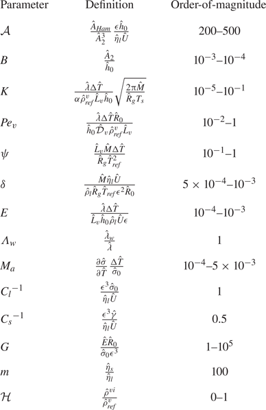
An estimation of the order-of-magnitude of certain dimensionless parameters is depicted in table 2.
Table 2. Order-of-magnitude estimate for the dimensionless parameters assuming  $\epsilon =0.1$,
  $\Delta \hat {T}=3$ K.
4. Evolution equations
In order to derive the evolution equations, we make an approximation that the streamwise displacement follows a parabolic profile in  $z$, since this is the simplest solution that satisfies (3.13) (Matar et al. Reference Matar, Gkanis and Kumar2005; Ghosh, Bandyopadhyay & Sharma Reference Ghosh, Bandyopadhyay and Sharma2016; Charitatos & Kumar Reference Charitatos and Kumar2020, Reference Charitatos and Kumar2021) for the soft solid,
 \begin{equation} u_x=b_1(x,t) z^2 + b_2(x,t) z +b_3(x,t), \end{equation}
in which  $b_1$,
  $b_2$ and
  $b_3$ are functions of both space and time that will be determined later; a detailed derivation is given in Appendix A.
Using the boundary condition at  $z=-H$, i.e.
  $u_x=0$, we get for
  $b_3(x,t)$ the following:
 \begin{equation} b_3=b_2 H - b_1 H^2. \end{equation}
Regarding the coefficient  $b_1(x,t)$, introducing (4.1) into the
  $x$-component of the solid momentum, i.e. (3.13), yields the following expression:
 \begin{equation} \frac{\partial b_1}{\partial t} = \frac{1}{m} \left(\frac{1}{2} \frac{\partial p_s}{\partial x} -G b_1 \right). \end{equation}
From (3.19), using (4.1) and (3.13), as well as the expression of the  $x$-component of the liquid velocity (i.e. (A9) derived in Appendix A), we conclude to an expression for the coefficient
  $b_2(x,t)$,
 \begin{equation} \frac{\partial b_2}{\partial t} = \frac{1}{m} \left( \frac{\partial p_l}{\partial x} (\xi-\zeta) - Gb_2 +( \epsilon^2 C_l )^{{-}1} \frac{\partial \sigma}{\partial x} \right). \end{equation}
In order to derive the evolution equation for  $\zeta (x,t)$, we use the kinematic equation for the liquid, i.e. (3.10). Using the expressions of
  $v_x$ and
  $v_z$ (i.e. (A9) and (A11), respectively, derived in Appendix A), and setting
  $z=\zeta$, we get
 \begin{align} \frac{\partial \zeta}{\partial t} &= \frac{\partial}{\partial x} \left[ \frac{1}{3} \frac{\partial p_l}{\partial x} (\zeta-\xi)^3 - \frac{1}{2} ( \epsilon^2 C_l )^{{-}1} \frac{\partial \sigma}{\partial x} (\zeta-\xi)^2 - H \zeta \left( \frac{\partial b_2}{\partial t} - H \frac{\partial b_1}{\partial t}\right) \right] \nonumber\\ &\quad + \xi \frac{\partial}{\partial x} \left(H \frac{\partial b_2}{\partial t} -H^2 \frac{\partial b_1}{\partial t}\right) + \frac{2 H^3}{3} \frac{\partial^2 b_1}{\partial x \partial t} - \frac{H^2}{2} \frac{\partial^2 b_2}{\partial x \partial t}- EJ. \end{align}
Using the expressions of the material derivatives of  $\xi$ and
  $u_z(x,0,t)$, (i.e. (A12) and (A13), respectively, derived in Appendix A), leads to an evolution equation for
  $\xi (x,t)$:
 \begin{equation} \frac{\partial \xi}{\partial t}+\frac{\partial \xi}{\partial x} \left( H \frac{\partial b_2}{\partial t}- H^2 \frac{\partial b_1}{\partial t}\right)=\frac{\partial}{\partial t} \left(\frac{2H^3}{3} \frac{\partial b_1}{\partial x}- \frac{H^2}{2} \frac{\partial b_2}{\partial x}\right). \end{equation}
Furthermore, we can easily find an evolution equation for the droplet thickness  $h(x,t)=\zeta (x,t)-\xi (x,t)$ by subtracting (4.6) from (4.5), as follows:
 \begin{equation} \frac{\partial h}{\partial t} + \frac{\partial q}{\partial x} ={-}EJ, \end{equation}
where the liquid flow rate,  $q$, is given by
 \begin{equation} q={-}\frac{1}{3}\frac{\partial p_l}{\partial x} (\zeta-\xi)^3 +\frac{1}{2} ( \epsilon^2 C_l )^{{-}1} \frac{\partial \sigma}{\partial x} (\zeta-\xi)^2+ H (\zeta-\xi) \left(\frac{\partial b_2}{\partial t}-H \frac{\partial b_1}{\partial t}\right). \end{equation}
By integrating the energy equation, i.e. (3.15), with respect to  $z$, and using the continuity of thermal flux at
  $z=\xi (x,t)$, i.e. (3.16) and the boundary condition,
  $T_w\vert _{-H}=0$, the following evolution equation for the temperature in the soft solid substrate can be derived:
 \begin{equation} T_w={-}\frac{J}{\varLambda_w}(z+H). \end{equation}
Similarly, by integrating the energy equation, (3.5), with respect to  $z$, and using the energy balance, (3.7), and the fact that
  $T |_\xi =T_w\vert _{\xi }$, the following evolution equation for the temperature in the liquid phase can be derived:
 \begin{equation} T={-}J (z-\xi)-\frac{J}{\varLambda_w}(\xi+H). \end{equation}
In summary, we solve numerically the evolution equations (4.3), (4.4), (4.6), (4.7) and (3.24) on the domain  $0< x< L_x$ and (3.21) on the two-dimensional domain
  $0< x< L_x$,
  $0< z< L_z$. The latter equation is subjected to boundary conditions (3.22) and (3.23) in the
  $z$-direction and to the following condition in the
  $x$-direction:
 \begin{equation} \left.\frac{\partial \rho_v}{\partial x} \right\vert_{x=0}= \left.\frac{\partial \rho_v}{\partial x} \right\vert_{x=L_x}=0. \end{equation}
The numerical solution of the evolution equations (4.3), (4.4), (4.6) and (4.7) is subjected to the following conditions at  $x=0$ and
  $x=L_x$:
 \begin{equation} \left. \begin{array}{c}
\displaystyle \dfrac{\partial \zeta}{\partial x} =
\dfrac{\partial \xi}{\partial x} = \dfrac{\partial^3
\zeta}{\partial x^3} = \dfrac{\partial^3 \xi}{\partial x^3}
= \dfrac{\partial b_1}{\partial x} = \dfrac{\partial
b_2}{\partial x} =0, \\ \zeta-\xi = \beta, \end{array}
\right\} \end{equation}
\begin{equation} \left. \begin{array}{c}
\displaystyle \dfrac{\partial \zeta}{\partial x} =
\dfrac{\partial \xi}{\partial x} = \dfrac{\partial^3
\zeta}{\partial x^3} = \dfrac{\partial^3 \xi}{\partial x^3}
= \dfrac{\partial b_1}{\partial x} = \dfrac{\partial
b_2}{\partial x} =0, \\ \zeta-\xi = \beta, \end{array}
\right\} \end{equation}
where  $\beta =\hat {\beta }/\hat {h}_0$ is the dimensionless precursor film height. These conditions were decided upon, after the assumptions that both
  $\zeta$ and
  $\xi$ are horizontal at
  $x=0$ and
  $x=L$ and that the dimensionless precursor film thickness is equal to the distance between the two interfaces at these positions. Furthermore, the liquid flow rate and the solid displacement in the
  $z$-direction were considered equal to zero at all ends.
Concerning the initial conditions, we assumed a flat liquid–solid interface at  $t=0$:
 \begin{equation} b_1(x,0)=b_2(x,0)=\xi(x,0)=J(x,0)=0. \end{equation}
As far as the initial shape of the droplet thickness is concerned, we use a fourth-order polynomial which satisfies  ${\partial h}/{\partial x} = {\partial ^3 h}/{\partial x^3} =0$ at the droplet centre (
 $x=x_{cm,l}$ or
  $x_{cm,r}$) and
  ${\partial h}/{\partial x} = 0$ as well as
  $h = \beta$ at distance
  $l_0$ from the droplet centre, respectively. The length and height of the computational domain was taken equal to
  $L_x=\hat {L}_x/\hat {R}_0=16$ and
  $L_z=\hat {L}_z/\hat {R}_0=5$, respectively. The dimensionless initial droplet footprint half-width,
  $l_0$, was defined equal to
  $l_0=1.5$ and the dimensionless initial droplet cross-sectional area was considered to be equal to
  $V=2/3$. Moreover, the initial centre of mass for each droplet was taken at
  $x=x_{cm,l}=4$ and at
  $x=x_{cm,r}=12$, hence the initial distance between the two centres of mass was given by
  $\Delta x_{cm}=x_{cm,r}-x_{cm,l}=8$, while the centre of mass of the system was initially located at
  $x=x_{cm,g}=8$.
The above set of equations were solved using the finite element method, and it was implemented in COMSOL Multiphysics commercial software. We applied a fully implicit finite difference scheme to solve the system of the evolution equations and we selected the PARDISO iterative solver for the intermediate time-stepping. Typically we use 10 000 elements for the discretisation of the system geometry and the moving mesh of the surrounding atmosphere was appropriately refined using free triangular cells; numerical checks showed that increasing the number of elements further led to negligible changes. The simulations stop when the system mass has decreased by 80 %.
5. Results and discussion
Droplet evaporation on compliant substrates is a parametrically rich problem. We begin our study by examining the case of the evaporation of a single droplet on a soft substrate in § 5.1, while in § 5.2 we proceed with simulations for a system of two interacting droplets. Numerical solutions were obtained over a wide range of parameter values. The ‘base’ case, however, has broadly typical values of  $\epsilon =0.1$,
  $l_0=1.5$,
  $H=0.1$,
  $A=500$,
  $B=0.005$,
  $n=3$,
  $c=2$,
  $E=10^{-4}$,
  $\mathcal {H}=0.5$,
  $K=0.2$,
  $\psi =0.1$,
  $Pe_v=0.1$,
  $\delta =10^{-3}$,
  $m=100$,
  $C_l^{-1}=1$,
  $C_s^{-1}=0.5$, unless noted otherwise in the text. In the figures that follow, we define a scaled time
  $t'=t/t_{ev}$ where
  $t_{ev}$ is defined as the time that the system mass has decreased by 80 %.
5.1. Evaporation of a single droplet
5.1.1. Effect of thermocapillarity
To set the stage, we begin with the simplest configuration, i.e. the evaporation of a single droplet on a soft substrate. Figure 2 depicts the typical time evolution of the liquid–gas and the liquid–solid interfaces for a single sessile evaporating droplet, highlighting the contact line region in the inset of the same figure. Charitatos & Kumar (Reference Charitatos and Kumar2021) considered a system similar to the present set-up, albeit ignoring the effect of thermocapillarity and employing the one-sided model. In order to examine the effect of thermocapillary phenomena, we present in figure 2(a) the evolution for  $M_a=0$ and in figure 2(b) for
  $M_a=0.005$. In the absence of thermocapillary stresses (figure 2a), in line with Charitatos & Kumar (Reference Charitatos and Kumar2021), we notice a gradual decrease in the droplet footprint, which is accompanied by a small deformation of the soft substrate, due to the balance of the capillary forces along the liquid–solid interface and in the contact line region. Consequently, a wetting ridge is formed and as the droplet dries out, both the contact line and the wetting ridge retract as a result of the decrease in the droplet volume.

Figure 2. Time evolution of the liquid–air ( $\zeta$) and the liquid–solid (
 $\xi$) interfaces for a single droplet for (a)
  $M_a=0$ (
 $t_{ev}=4242$) and (b)
  $M_a=5\times 10^{-3}$ (
 $t_{ev}=5366$), respectively, for
  $G=3$. The inset is an enlargement of the contact line region. The rest of the system parameters are the same with the ‘base’ case.
On the other hand, in the presence of thermocapillarity (see figure 2b), the Marangoni stresses drive liquid towards the colder region (i.e. at droplet apex, see figure 3b) causing a faster retraction of the droplet. The faster motion of the contact line results in significantly larger substrate deformation, since for example at  $t=100$ the maximum deformation of the wetting ridge (evaluated as the
  $z$-position of the contact line, see figure 1c), is
  $\xi _{max}= 0.038$ and
  $\xi _{max}= 0.068$, in figures 2(a) and 2(b), respectively. Furthermore, it can be deduced from figure 2(b) that for finite values of
  $M_a$ the loss of droplet mass is retarded;
  $t_{ev}$ is considerably larger in figure 2(b) as compared with figure 2(a). This is due to the fact that the action of thermocapillary stresses leads to a considerably smaller droplet footprint with larger distance of the droplet apex from the rigid solid (at
  $z=-H$). The increased droplet height inhibits the supply of heat from the substrate (maintained at a constant temperature) to the interface, which is continuously being cooled due to the effect of latent heat. This consequently leads to lower temperature along the liquid–gas interface and in turn results in the overall decrease of the evaporation rate; the evolution of the local evaporation flux is presented in figure 3(a).

Figure 3. Time evolution of (a) the evaporation rate  $J$ and (b) the interfacial temperature
  $T_s$, for a single droplet for
  $M_a=5\times 10^{-3}$ and
  $G=3$ (
 $t_{ev}=5366$).The rest of the system parameters are the same with the ‘base’ case.
To illustrate the vapour concentration field in the gas phase, we present the corresponding contour plot in figure 4, for the case of  $M_a=0.005$. It is noted that the far-field boundary is taken to be very far from the droplet (i.e. at
  $z=\epsilon ^{-1} z'=50$) and as a result the droplet is difficult to see in this figure. We notice, though, that in the neighbourhood of the droplet the vapour concentration is high and decreases moving away from the droplet, as expected.

Figure 4. Gas phase concentration profiles at different time instants for  $M_a=5\times 10^{-3}$ and
  $G=3$: (a)
  $t'=0$; (b)
  $t' = 0.02$; (c)
  $t'=0.4$; (d)
  $t'=0.8$. The rest of the system parameters are the same with the ‘base’ case.
5.1.2. Effect of substrate elasticity and thickness
Here, we examine the effect of elasticity of the substrate by varying  $G={\hat {E} \hat {R}_0}/{\hat {\sigma }_0 \epsilon ^3}$; this parameter measures the ratio of elastic to liquid–gas interfacial tension forces. Here
  $G$ is proportional to the shear modulus of the soft solid and therefore smaller values correspond to the case of softer substrates. By letting
  $G\rightarrow \infty$, the case of the rigid substrate can be recovered. In figure 5(a), we investigate the effect of substrate elasticity on the deformation of the soft solid, by plotting the evolution of the maximum deformation of the wetting ridge,
  $\xi _{max}$, with time. Naturally, it can be seen that the softer substrates deform more easily. Figures 5(b) and 5(c) depict the time evolution of the contact radius and the apparent contact angle, respectively, of a single droplet evaporating on a rigid (
 $G=10^7$) and on soft solid substrates with
  $G=1$, 3, 10, 100. Following the work of Charitatos & Kumar (Reference Charitatos and Kumar2021), the apparent contact angle is defined as the largest angle between the tangent of the liquid–air interface,
  $z=\zeta (x,t)$ and
  $z=0$. On the other hand, the contact radius is defined as the intersection point between the tangent of the largest angle and
  $z=0$.

Figure 5. Time evolution of (a) the point of maximum deformation of the wetting ridge  $\xi _{max}$, (b) the contact radius
  $r$ and (c) the apparent contact angle
  $\theta$ for a single droplet, varying substrate elasticity
  $G$ and for
  $M_a=0.005$. (d) Space–time plot of the droplet profiles at a soft substrate with
  $G=1$ and for
  $M_a=0.005$. The inset is a magnified view of the wetting ridge profiles during droplet spreading. The rest of the system parameters are the same with the ‘base’ case.
At early times and for all examined cases, the droplet contact radius quickly decreases (figure 5b), accompanied by an increase in the apparent contact angle (figure 5c), while in parallel the size of the wetting ridge grows (figure 5a). The initial droplet retraction, which is due to both droplet evaporation and the action of thermocapillary stresses, takes place faster for softer substrates. After the initial droplet retraction, the contact line remains apparently pinned for a significant amount of time ( $t \approx 3- 300$) with a relatively constant droplet footprint, indicating the stick-phase of the droplet spreading (see inset of figure 5d). In fact, in the case of softer substrates (i.e.
  $G=1$) the constant contact radius (CCR) is maintained throughout evaporation accompanied with a continuous decrease of the contact angle (see figure 5c); the evaporation takes place in CCR mode. In contrast, for harder substrates (i.e.
  $G \geq 10$) the evaporation takes place in constant contact angle (CCA) mode, with a continuous slow decrease of the contact radius, in line with previous computational studies referring to droplet evaporation on rigid substrates (Pham & Kumar Reference Pham and Kumar2017). This CCR mode observed in softer substrates has been previously reported in experimental studies concerning the evaporation of water droplets on compliant PDMS substrates (Lopes & Bonaccurso Reference Lopes and Bonaccurso2012; Gerber et al. Reference Gerber, Lendenmann, Eghlidi, Schutzius and Poulikakos2019). After depinning, the contact line retracts continuously until the droplet fully evaporates. At the same time a non-monotonic behaviour of the contact angle is observed in line with previous experimental studies of Lopes & Bonaccurso (Reference Lopes and Bonaccurso2012, Reference Lopes and Bonaccurso2013) and Yu et al. (Reference Yu, Wang and Zhao2013).
In figure 6(a), we investigate the effect of substrate thickness on the deformation of the soft solid, by plotting the maximum deformation of the wetting ridge,  $\xi _{max}$, with time. It can be seen that the thicker substrates deform more easily than the thinner ones. Clearly, this is due to the fact that with decreasing thickness of the compliant substrate, less soft solid is available to deform, thereby increasing the resistance to the deformation of the substrate and leading to smaller wetting ridges. Consequently, making the substrate thinner can be seen as equivalent to making it more rigid, whereas thicker substrates behave similarly to softer ones. This effect is also reflected in the mode of evaporation. As it can be seen in figure 6(b), evaporation takes place in CCR mode for the thicker, hence softer, substrate (
 $H=10^{-1}$), and in CCA mode for the thinner, hence harder, substrate (
 $H=10^{-3}$), in line with the findings shown in figure 5.

Figure 6. Time evolution of (a) the point of maximum deformation of the wetting ridge  $\xi _{max}$ and (b) the apparent contact angle
  $\theta$ for a single droplet, varying substrate thickness
  $H$ and for
  $G=1$,
  $M_a=0.005$. The rest of the system parameters are the same with the ‘base’ case.
5.2. Evaporation of a pair of droplets
Now that we have studied the basic characteristics of the flow for a single sessile evaporating droplet, we may proceed with the examination of a system of multiple volatile droplets. In particular, we will investigate the dynamics of a pair of droplets and focus on the effects of their interaction, either through the soft substrate or their atmosphere, on the dynamics of the drying process.
In figure 7, we depict the time evolution of a pair of droplets evaporating on a compliant substrate with  $G=1$. In these simulations, we fully take into account the effect of thermocapillarity and examine two cases with
  $M_a=0.001$ and
  $M_a=0.005$ in figures 7(a) and 7(b), respectively. An interesting observation is that in both cases the droplets appear to move away from each other as they dry out. Regarding the deformation of the liquid–solid interface near the two contact lines, we observe that for low values of
  $M_a$ the height of the left and the right wetting ridge of each droplet is nearly symmetric (see inset of figure 7a), whereas for higher values of
  $Ma$ the droplet deforms asymmetrically with the deformation of the soft solid in the inner region between the two droplets being somewhat smaller than the deformation in the outside region (see inset of figure 7b). These observations provide a clear indication of the interaction of two droplets which may communicate either through the gas phase or through the developed stresses in the underlying viscoelastic substrate.

Figure 7. Time evolution of the liquid–air ( $\zeta$) and the liquid–solid (
 $\xi$) interfaces for two droplets drying on a soft substrate with
  $G=1$ and for (a)
  $M_a=0.001$ (
 $t_{ev}=4667$) and (b)
  $M_a=0.005$ (
 $t_{ev}=5889$), respectively. The inset is an enlargement of the height range of the contact line region of the left drop at
  $t'=0.4$. The rest of the system parameters are the same with the ‘base’ case.
5.2.1. Effect of the gas phase and thermocapillarity
In order to shed light on the physical mechanisms behind the observed dynamics, we will first focus on the gas phase and depict in figure 8 the vapour concentration in the atmosphere of the two droplets. As shown in this figure, the vapour concentration is higher between the two droplets than in their periphery. Since the evaporation flux is limited by diffusion (see (3.23)), the higher saturation of the gas phase with vapour in the region between the two droplets results in weaker evaporation in that region; the spatial dependence of the evaporation flux  $J$ is plotted in figure 9(a). For all values of
  $Pe_v$ that we have examined,
  $J$ acquires an asymmetric profile along the liquid–gas interface of each droplet; this can be seen more clearly by plotting
  $\partial J / \partial x$ in the inset of the same figure for
  $Pe_v=0.1$.

Figure 8. Gas phase concentration profiles at different time instants for  $G=1$ and
  $M_a=0.005$: (a)
  $t'=0.002$; (b)
  $t'=0.02$; (c)
  $t'=0.08$; (d)
  $t'=0.2$; (e)
  $t'=0.5$; (f)
  $t'=0.8$; (
 $t_{ev}=5889$). The rest of the system parameters are the same with the ‘base’ case.

Figure 9. Effect of  $Pe_v$ on the spatial profile of (a) the evaporation rate
  $J$, (b) the interfacial temperature
  $T_s$, (c) the Marangoni stresses,
  $h({\partial \sigma }/{\partial x})$, at
  $t'=0.5$. (d) The time evolution of the distance between the droplets’ centres of mass,
  $\Delta x_{cm} = x_{cm,r}-x_{cm,l}$ for
  $G=1$,
  $M_a=0.005$ and the rest of the system parameters are the same with the ‘base’ case. The insets in (a) and (b) depict the spatial profiles for
  $Pe_v=0.1$ of
  $\partial J / \partial x$ and
  $\partial T_s / \partial x$, respectively.
Due to the effect of the latent heat, the evaporation flux affects the local interfacial temperature, which is depicted in figure 9(b); the liquid–gas interface is cooler than the rest of the drop and the interfacial temperature is lowest at the droplet apex. The presence of temperature gradients affects in turn the flow field inside the droplet due to the action of Marangoni stresses, the spatial dependence of which, is plotted in figure 9(c); the Marangoni stress is proportional to  $h \partial \sigma / \partial x$. Focusing first on each droplet, we notice that the Marangoni stresses, exhibiting opposite signs in the regions left and right from the droplet apex, act as a compressive force reducing the footprint of the droplet. The effect of thermocapillarity on the droplet footprint is shown very clearly in figure 10(a) where we plot the length of footprint of the left drop,
  $\Delta x_{cl}$ (see also figure 1c), defined as the distance between the maxima of the left and right wetting ridge. Additionally, the asymmetric profile of the evaporation flux along the liquid–gas interface also induces a symmetry breaking in the interfacial temperature profile; this is clearly shown in the inset of figure 9(b) where we plot the spatial dependence of
  $\partial T_s / \partial x$ for the droplet on the left-hand side of the domain for
  $Pe_v=0.1$.

Figure 10. Time evolution of (a) the length of footprint of the left drop,  $\Delta x_{cl}$, (b) the distance between the two centres of mass,
  $\Delta x_{cm}$, and (c) the system mass, for different values of
  $M_a$ and for
  $G=1$. The rest of the system parameters are the same with the ‘base’ case.
As a result, the Marangoni stresses not only compress the droplet but also contribute to their repulsion. This is demonstrated in figure 10(b) where we plot the evolution of the distance between the centres of mass of the droplets on the left-hand and the right-hand side of the domain,  $\Delta x_{cm}=x_{cm,r}-x_{cm,l}$ (see also figure 1c), with time for different values of
  $M_a$. A similar effect is also shown in figure 9(d) where enhanced repulsion is found for lower values of
  $Pe_v$; increase of
  $Pe_v$ corresponds to slower vapour diffusion enhancing the difference in the evaporation flux between the two sides of the droplets as shown in figure 9(a). Regarding the droplet lifetime, thermocapillarity plays a dual role; on one hand enhancing the evaporation rate in the region between the two droplets, as they move away from each other, but at the same time reducing the overall evaporation due to the compressive action of Marangoni stresses on the droplets. As it can be seen in figure 10(c), where we plot the total mass of the system, the droplet lifetime increases considerably with
  $M_a$, thus indicating that the latter effect is more significant.
5.2.2. Effect of substrate elasticity in the absence of thermocapillarity
In order to investigate the effect of the substrate elasticity, we plot in figure 11 the time evolution of a pair of droplets evaporating on solid substrates with  $G=10$, 500,
  $10^5$; here, we neglect the effect of Marangoni stresses, i.e.
  $M_a=0$. Interestingly, we find that in the case of soft substrates the droplets repulse as they dry out (see figure 11a), whereas in the case of stiffer substrates the droplets are attracted to each other (see figure 11b). We note that in the latter case the droplets approach each other but do not coalesce; this behaviour is found in a well-defined range of
  $G$ (i.e.
  $300 \leq G \leq 2 \times 10^4$ for
  $Ma=0$ and
  $2 \times 10^3 \leq G \leq 5 \times 10^4$ for
  $Ma=10^{-4}$). For very stiff substrates (see figure 11c for
  $G=10^5$), the two droplets eventually coalesce, and the drying process continues as for a single droplet. The dynamics for these three cases is also presented in the form of space–time plots in figure 12 (see figure 12a, figure 12c and figure 12d for
  $G=10$, 500 and
  $10^5$, respectively).

Figure 11. Time evolution of the liquid–air ( $\zeta$) and the liquid–solid (
 $\xi$) interfaces for two droplets with (a)
  $G=10$ (
 $t_{ev}=4537$), (b)
  $G=500$ (
 $t_{ev}=4934$) and (c)
  $G=10^5$ (
 $t_{ev}=5048$), respectively, for
  $M_a=0$. The inset is an enlargement of the height range of the contact line region of the left drop at
  $t'=0.4$. (d) Time evolution of the system mass, varying substrate elasticity
  $G$. The rest of the system parameters are the same with the ‘base’ case.

Figure 12. Space–time plots of the droplet profiles for (a)  $G=10$, (b)
  $G=100$, (c)
  $G=500$, (d)
  $G=10^5$, (e)
  $G=10^6$ and (f)
  $G=10^7$, for
  $M_a=0$. The rest of the system parameters are the same with the ‘base’ case.
Inspecting the space–time plots presented in figure 12 and comparing with the work of Henkel et al. (Reference Henkel, Snoeijer and Thiele2021) for non-volatile droplets, we notice a significant difference. For all the cases of volatile droplets that we have examined, varying the softness of the substrate, we find that mass transfer from one drop to the other does not take place and hence there is no droplet coarsening through the Ostwald ripening mode; the latter mode was found to be dominant in the study of Henkel et al. (Reference Henkel, Snoeijer and Thiele2021). For substrates with  $G=10^5$ where droplets coalesce, the coarsening process takes place with a typical translation mode as shown in figure 12(d). After the two contact lines of the neighbouring droplets come in contact, there is fast droplet coalescence. This is in contrast to the case shown in figure 12(c) (
 $G=500$) where after the two adjacent contact lines touch each other, the droplets do not coalesce. Furthermore, we note that in parallel to the results of Henkel et al. (Reference Henkel, Snoeijer and Thiele2021), the translation mode which defines exclusively the coarsening behaviour in figure 12(d) leads to a symmetric movement of the droplets towards each other, without displacing the system centre of mass (see also figures 11c and 13b). To check whether our model can capture the emergence of Ostwald ripening in the case of non-volatile droplets, we further examine in figure 14(a) the limit of negligible evaporation (
 $E=10^{-8}$) for a substrate with high rigidity (
 $G=10^7$); the equilibrium contact angle is taken to be approximately equal to
  $44^\circ$ (
 $A=120$) in order to consider a system with similar wetting characteristics as in Henkel et al. (Reference Henkel, Snoeijer and Thiele2021). As it is clearly shown in this figure, in the limit of non-volatile droplets the Ostwald ripening emerges at late times, as expected, with mass transferring from one drop to the other until the smaller droplet vanishes, and all the mass is contained in the larger remaining droplet. On the other hand, in figure 14(b) we examine the same system with two volatile droplets (
 $E=10^{-4}$). As shown, evaporation takes place on much faster time scales and coalescence eventually occurs with the translation mode.

Figure 13. Time evolution of (a) the distance between the two centres of mass  $\Delta x_{cm}$ and (b) the centre of mass of the system
  $x_{cm,g}$, for
  $M_a=0$. The rest of the system parameters are the same with the ‘base’ case.

Figure 14. Space–time plots of the droplet profiles for (a)  $E=10^{-8}$ and (b)
  $E=10^{-4}$, for
  $M_a=0$ and
  $G=10^7$. The domain length is
  $L=48$,
  $\mathcal {A}=120$ and the rest of the system parameters are the same with the ‘base’ case.
As explained by Karpitschka et al. (Reference Karpitschka, Pandey, Lubbers, Weijs, Botto, Das, Andreotti and Snoeijer2016), interaction of non-volatile droplets on the surface of elastic solids is determined by the balance of elasticity and capillary forces and the resulting local deformation of the soft solid in the contact line region. Depending on the stiffness (or thickness) of the substrate, the elastic meniscus in the contact line region between the two droplets rotates by an angle as compared with the meniscus of an isolated drop and the direction of the rotation determines whether the drop–drop interaction is attractive or repulsive. In the case of drying droplets, though, the shape of the wetting ridge is not determined merely by elastocapillary phenomena but can also be significantly affected by the local evaporation rate (see the relevant discussion in Charitatos & Kumar (Reference Charitatos and Kumar2021)). Given the fact that the evaporation mass flux between the two contact lines of each droplet differs, this will also contribute to the imbalance of forces between the inner and outer contact lines, thereby affecting the mode of droplet interaction. To examine in more detail the complex droplet dynamics of our system, we plot in figure 13(a) the evolution of the distance between the centre of mass of the droplets,  $\Delta x_{cm}$, with time. It can be seen that in the case of soft substrates (
 $G \leq 100$) the droplets repulse, since
  $\Delta x_{cm}$ continuously increases throughout evaporation. For harder substrates (
 $G>100$), though, the imbalance acts in the opposite direction pushing the droplets towards each other. In the case of nearly rigid substrates (
 $G \geq 10^6$), the deformation of the viscoelastic solid is so small that this imbalance does not play an important role and thus the distance between the two droplets does not change significantly during evaporation.
The different modes of the drying process affect also the lifetime of the droplets. As shown in figure 11(d), the evaporation is faster in softer substrates, due to the increased distance between the two droplets and the fact that a smaller amount of vapour is trapped amidst the repulsing droplets leading to enhanced evaporation fluxes. In contrast, the greater amount of vapour trapped amidst the droplets when they attract in stiffer substrates, retards the evaporation significantly. Moreover, we notice that although for soft substrates the symmetry of the system is preserved throughout the drying process, this is not the case for substrates with intermediate stiffness. In fact, as it can be seen in figure 11(b) (and figure 12c), the pair of droplets at late stages of evaporation starts moving to the left exhibiting a clear symmetry breaking; the mechanisms for this behaviour will be investigated in detail below. Similarly, as shown in figure 11(c) (and figure 12d) for  $G=10^5$, the droplet that has emerged after the coalescence of the two droplets appears to move slightly to the right, also indicating a symmetry breaking of the system, albeit with a somewhat smaller droplet displacement from the system centre of mass.
As noted above, the elasticity of the substrate affects not only the relative distance between the droplets but may also lead under conditions to a symmetry breaking with the centre of mass of the system,  $x_{cm,g}$ being displaced from its initial position, i.e. the droplets appear to be ‘walking’ along the viscoelastic substrate. In figure 13(b), we depict the effect of
  $G$ on the evolution of the position of the system centre of mass,
  $x_{cm,g}$. As shown in this figure, for very soft and very hard substrates (i.e.
  $G=10$ and
  $G \geq 10^6$) the centre of mass of the system remains at
  $x_{cm,g}=8$ and the symmetry is preserved throughout the drying process. This is not the case, though, for substrates with intermediate stiffness where symmetry breaking is found; we note that the system symmetry is considered broken when the centre of mass of the system has moved
  $\pm$10 % of its initial maximum height (i.e. 0.1 dimensionless distance) from its initial position. It should be pointed out that these asymmetric solutions are spontaneous and emerge due to disturbances of the numerical finite element scheme, while they appear to be stable with the increase in mesh resolution. To make sure that the symmetry breaking is not artificially introduced by the imposed boundary conditions, we varied the size of the domain or even applied periodic boundary conditions in the
  $x$-direction; these efforts are presented in detail in Appendix B. As discussed therein, neither the type of imposed boundary conditions or the domain size qualitatively affect the observed droplet behaviour. It is important to note that a spontaneous symmetry breaking has been also a matter of interest in earlier experimental and computational studies (Hernández-Sánchez et al. Reference Hernández-Sánchez, Lubbers, Eddi and Snoeijer2012; Leong & Le Reference Leong and Le2020) of non-volatile droplets; Leong & Le (Reference Leong and Le2020) examined the growth of an inflating droplet on viscoelastic soft substrate and also observed asymmetric solutions for substrates with intermediate stiffness.
5.2.3. Effect of substrate elasticity in the presence of thermocapillarity
Next, we take into account the effect of thermocapillary stresses. In figure 15, we depict the droplet dynamics for  $M_a=0.005$ and three different values of
  $G=1$, 50, 500. Regardless of the elasticity strength of the substrate, it is shown that in all cases the droplets repulse from each other. This behaviour is markedly different from the one discussed previously in the absence of thermocapillary effects where the droplets are attracted to each other for substrates with intermediate or high values of
  $G$. As discussed in figure 10, the Marangoni stresses play a dual role both acting as to compress the droplet footprint and also contributing to droplet repulsion. As shown in figure 16(a) where we plot the distance
  $\Delta x_{cm}$ between the two droplets for a wide range of
  $G$ values for
  $M_a=0.005$, the latter contribution is dominant and thus always leading the droplets to repulse from each other at the early stages of the drying process. Nevertheless, we notice that at later stages and for substrates with intermediate values of
  $G$ (i.e. for
  $G=50$, 500, 2000,
  $10^4$) the droplet distance eventually starts decreasing indicating that the droplets are attracted to each other. This can be attributed to the fact that, at these late stages of the drying process, the droplet distance has increased considerably allowing the vapour concentration to acquire a more uniform profile along the interface of each droplet, leading to a more uniform evaporation flux and in turn to smaller temperature gradients. As a result, the thermal Marangoni stresses are significantly reduced, while the capillary forces induced by the substrate elasticity become dominant and drive the droplets closer to each other. For harder substrates, the capillary forces, as explained above, are weaker due to the fact that the substrate is less susceptible to elastic deformations and therefore the droplets continue to repulse due to the action of Marangoni stresses throughout the drying process.

Figure 15. Time evolution of the liquid–air ( $\zeta$) and the liquid–solid (
 $\xi$) interfaces for two droplets with (a)
  $G=1$ (
 $t_{ev}=5889$), (b)
  $G=50$ (
 $t_{ev}=5329$) and (c)
  $G=500$ (
 $t_{ev}=5222$), respectively, for
  $M_a=0.005$. The inset is an enlargement of the height range of the contact line region of the left drop at
  $t'=0.4$. (d) Time evolution of the system mass varying substrate elasticity
  $G$. The rest of the system parameters are the same with the ‘base’ case.

Figure 16. Time evolution of (a) the distance between the two centres of mass  $\Delta x_{cm}$ and (b) the centre of mass of the system
  $x_{cm,g}$, for
  $M_a=0.005$. (c) The contribution of the Marangoni stresses and capillary forces in the average
  $x$-velocity of droplet 1 and 2 for
  $G=500$ and
  $M_a=0.005$. The rest of the system parameters are the same with the ‘base’ case.
Interestingly, we also notice in figure 15(c), i.e. for a substrate with intermediate stiffness ( $G=500$), that the droplets initially repulse, then they are attracted and eventually symmetry breaking takes place; in figure 15(c), a dashed arrow is drawn to indicate the motion of each droplet. As shown in figure 16(b) where we plot the evolution of the global centre of mass
  $x_{cm,g}$ with time, we find that the symmetry is preserved only for extremely soft and extremely stiff substrates, while for intermediate values of
  $G$ the droplets appear to ‘walk’ along the substrate. It should be noted that the emergence of this symmetry breaking at late stages of evaporation takes place spontaneously (i.e. at no specific time instant) and there is no preferred direction; it is triggered by numerical disturbances and appears to be stable and persistent with the increase in mesh resolution.
In figure 16(c), we make an effort to rationalise and elucidate the mechanisms responsible for the symmetry breaking, shown in figure 15(c) (i.e. for  $M_a=0.005$ and
  $G=500$). In order to examine the contribution of various forces, i.e. capillary, Marangoni and elastic, on the motion of the droplets, we evaluate their contributions to the mean velocity in the
  $x$-direction of each droplet, as follows:
 \begin{equation} \bar{v} =\frac{\displaystyle\int_{x_{cl}}^{x_{cr}} \int_0^h v_x \,{\rm d}z\,{{\rm d}\kern0.7pt x}} {\displaystyle\int_{x_{cl}}^{x_{cr}} h \,{{\rm d}\kern0.7pt x}} = \bar{v}_{cap,l}+\bar{v}_{cap,s}+\bar{v}_{Ma}+\bar{v}_{el}. \end{equation}
The terms  $\bar {v}_{cap,l}$ and
  $\bar {v}_{cap,s}$ denote the contributions from the capillary forces along the liquid–gas and liquid–solid interfaces, respectively, while the term
  $\bar {v}_{el}$ corresponds to the contribution of the elastic stresses and
  $\bar {v}_{Ma}$ corresponds to the contribution of the Marangoni stresses; the analytical expressions for the various contributions are given in Appendix C. We note that for a number of different cases that we have examined the dominant contributions come from the capillary forces and the Marangoni stresses along the liquid–gas interface, evaluated by the terms
  $\bar {v}_{cap,l}$ and
  $\bar {v}_{Ma}$, respectively;
  $\bar {v}_{cap,s}$ and
  $\bar {v}_{el}$ were typically found to be two orders of magnitude smaller than
  $\bar {v}_{cap,l}$ and
  $\bar {v}_{Ma}$, and thus neglected here. Nevertheless, it is important to note that despite the fact that
  $\bar {v}_{el}$ is typically very small, substrate elasticity implicitly contributes to the effect of capillary forces of the liquid–gas interface through the induced deformation of the contact line region. The time evolution of
  $\bar {v}_{cap,l}$ and
  $\bar {v}_{Ma}$ is depicted in figure 16(c) for both droplets; indexes 1 and 2 correspond to the droplet on the left and right, respectively.
At early times (i.e. approximately for  $t<800$), the contribution of the capillary and Marangoni stresses have similar magnitudes in both droplets and the symmetry is preserved (see figure 16b). The capillary forces act antagonistically with the Marangoni stresses pushing the droplets in opposite directions. The droplets, however, repulse due to the slightly higher magnitude of the Marangoni contribution. At later times (i.e. for
  $t>800$), a disturbance in the local deformation of the solid causes an imbalance between the two droplets (see figure 16c) leading to symmetry breaking and driving the system centre of mass away from its initial position.
From figure 16(b), it becomes evident that whether some disturbance will lead to a symmetry breaking or not, is a matter of the substrate elasticity. On the one hand, when the substrate is soft, it is very flexible and its deformation is very large. The size of an arising disturbance is insignificant compared with the size of the total substrate deformation and, as a result, the system centre of mass will remain constant and the symmetry will be preserved. On the other hand, in extremely stiff substrates, the deformation of the liquid–solid interface is very small, quickly damping any possible disturbance that could lead to an imbalance between the two droplets. However, at intermediate values of substrate elasticity, there can be a competition between this disturbance and the substrate deformation, which might eventually lead to an imbalance in the induced capillary and Marangoni stresses between the two droplets and thus to a symmetry breaking, if the size of the disturbance grows considerably as compared with the substrate deformation.
6. Conclusions
In this paper we have studied the two-dimensional dynamics of a system of one or two droplets evaporating on a viscoelastic solid substrate. Lubrication theory is used to simplify the equations of mass, momentum, energy and the force balances applied in the liquid and the solid phases, considering the Kelvin–Voigt model to account for substrate viscoelasticity. Our model takes into consideration the effect of thermal Marangoni stresses, as well as the droplet interaction through both the compliant substrate and the surrounding vapour. The model accounts for the presence of the vapour employing a two-sided approach and considering the diffusion-limited model. The contact line is modelled assuming a precursor film ahead of the droplet.
We have carried out a parametric study to investigate how the evaporation process, the flow dynamics and the interaction of droplets are affected by the physical properties of the compliant substrate (e.g. thickness, shear modulus) and vapour diffusion in the atmosphere affecting the local evaporation rate. In the case of a single droplet, it was found that for thinner substrates the elastic effects become decreasingly important and thus making the substrate thinner can be seen as equivalent to making it more rigid. Moreover, it is shown that on softer (or thicker) substrates the solid deforms affecting the wetting of the droplet and promoting evaporation in CCR mode, in line with experimental observations in the literature (Lopes & Bonaccurso Reference Lopes and Bonaccurso2012, Reference Lopes and Bonaccurso2013; Yu et al. Reference Yu, Wang and Zhao2013; Gerber et al. Reference Gerber, Lendenmann, Eghlidi, Schutzius and Poulikakos2019); the CCA mode is observed for harder (or thinner) substrates. Lastly, the effect of evaporative cooling and the action of thermocapillary stresses lead to smaller droplet footprints, resulting in an overall decrease of the evaporation rate, capturing the trend observed in earlier studies (Dunn et al. Reference Dunn, Wilson, Duffy, David and Sefiane2009b; Talbot et al. Reference Talbot, Berson, Brown and Bain2012; Schofield et al. Reference Schofield, Wilson, Pritchard and Sefiane2018) in the case of rigid substrates. On the other hand, in the case of a system of a pair of volatile droplets, it is shown that the droplets may communicate both through the viscoelastic substrate and the induced deformations of the liquid–solid interface and also through the vapour that diffuses in the atmosphere of the droplets. The delicate interplay between the elastic stresses in the substrate, the capillary pressure and the thermal Marangoni stresses determine the mode of droplet interaction.
To summarise the rich dynamics of this complex system, we produced the parametric map of the dynamic regimes depicted in figure 17, varying the values of Marangoni number,  $M_a$, and substrate elasticity
  $G$. In order to characterise the different regimes of the map, we consider that the system symmetry is broken when the centre of mass of the system has moved
  $\pm$10 % of the initial maximum droplet height (i.e. 0.1 dimensionless distance) from its initial position. In the absence of thermocapillary stresses (i.e.
  $M_a=0$), the droplets repulse on soft substrates (region I) whereas they are attracted to each other (and even coalesce) on stiff substrates (region VI) with symmetry breaking arising in the case of substrates with intermediate stiffness (region V). Droplet coalescence that takes place for substrates with intermediate stiffness closely resemble the translation mode of droplet coarsening observed for intermediate elasticity in Henkel et al. (Reference Henkel, Snoeijer and Thiele2021). The translation mode is mediated by elastic deformation recovering the inverted Cheerios effect (Karpitschka et al. Reference Karpitschka, Pandey, Lubbers, Weijs, Botto, Das, Andreotti and Snoeijer2016). On very stiff and very soft substrates, however, the dominance of the Ostwald ripening effect found by Henkel et al. (Reference Henkel, Snoeijer and Thiele2021) in the case of non-volatile droplets is significantly suppressed, due to the effect of evaporation that suppresses mass transfer between the droplets. Themocapillarity, on the other hand, apart from being responsible for the asymmetry of the wetting ridges on the two sides of each droplet between the two contact lines of each droplet, has also a drastic effect on the dynamics of the two droplets causing the repulsion of the droplets at the early stages of the drying process, irrespective of the stiffness of the viscoelastic solid (regions I, II and III). For substrates with intermediate stiffness, though, the droplet repulsion may also be followed by a phase of droplet attraction at later stages of the evaporating process (regions II and III), and under conditions to a symmetry breaking (region III); the symmetry is preserved either for very soft or very stiff substrates (regions I, II). Spontaneous symmetry breaking was also found in the study of Leong & Le (Reference Leong and Le2020) who examined the coalescence of inflating droplets on viscoelastic substrates, indicating that these systems are prone to instability as a result of the delicate interplay amongst elastic, capillary and Marangoni forces.

Figure 17. Map of the dynamic regimes depending on the value of Marangoni number,  $M_a$, and substrate elasticity
  $G$. The rest of the system parameters are the same with the ‘base’ case. We note that the borders in this map have been added as a visual guide and are not precise.
Our findings clearly indicate that the flow dynamics can be very interesting with important implications for the optimal design of soft substrates for controlled evaporation of droplets. Our comprehensive model can be easily extended to more realistic set-ups such as the simulation of multiple three-dimensional droplets or more complex systems such as the evaporation of particle-laden droplets. We believe that the present work should be complemented in the future with detailed experimental studies. To the best of our knowledge, such studies are lacking, despite the vast amount of experimental work that exists on evaporating droplets on rigid substrates.
Acknowledgements
We kindly thank the anonymous reviewers for their constructive comments.
Funding
The authors gratefully acknowledge the financial support received from the Hellenic Foundation for Research and Innovation (HFRI) and the General Secretariat for Research and Technology (GSRT), under grant agreement no. 792.
Declaration of interests
The authors report no conflict of interest.
Data availability
The data that support the findings of this study are available from the corresponding author, upon reasonable request.
Appendix A. Detailed derivation of the evolution equations for the soft substrate
The displacement in the  $z$-direction, i.e.
  $u_z(x,t)$, can be evaluated by integrating the continuity equation for the solid, i.e. (3.12):
 \begin{equation} u_z=b_4(x,t) - \left(\frac{\partial b_1}{\partial x} \frac{z^3}{3}+ \frac{\partial b_2}{\partial x} \frac{z^2}{2} + \frac{\partial b_3}{\partial x} z \right). \end{equation}
In the above equation,  $b_4(x,t)$ can be determined by using the fact that the displacement of the soft substrate at the interface with the rigid solid at
  $z=-H$ is zero and also using (4.2):
 \begin{equation} b_4 = \frac{\partial b_1}{\partial x} \left(\frac{2H^3}{3}\right)+ \frac{\partial b_2}{\partial x} \left(\frac{-H^2}{2}\right). \end{equation}
Introducing (A2) into (A1) we get the following expression for  $u_z$:
 \begin{equation} u_z = \frac{\partial b_1}{\partial x} \frac{1}{3} (2H^3 +3zH^2 -z^3) - \frac{\partial b_2}{\partial x} \frac{1}{2} {(z+H)}^2. \end{equation}
At any time instant, the position of the liquid–solid interface, i.e.  $\xi (x,t)$, is equal to the soft solid deformation at
  $z=0$ (i.e. the position of the undeformed liquid–solid interface) and therefore from (A3) we get
 \begin{equation} \xi(x,t)=u_z(x,0,t)= \frac{\partial b_1}{\partial x} \frac{2H^3}{3} - \frac{\partial b_2}{\partial x} \frac{H^2}{2}. \end{equation}
Turning our attention to the liquid phase, by integrating the  $x$-component of the momentum, i.e. (3.3), we get the following expression for
  $v_x$:
 \begin{equation} v_x = \frac{\partial p_l}{\partial x} \frac{z^2}{2} +f_1 z +f_2. \end{equation}
Integrating the continuity equation for the liquid, i.e. (3.2), and using (A5) we get an expression for  $v_z$:
 \begin{equation} v_z ={-}f_3- \int_{0}^{z} \frac{\partial v_x}{\partial x} \,{\rm d}z. \end{equation}
In (A5),  $f_1(x,t)$ is determined by taking the derivative of
  $v_x$ with respect to
  $z$ and by setting
  $z=\zeta (x,t)$. Using the expression for
  ${\partial v_x}/{\partial z}\vert _{\zeta }$ from the tangential stress balance in the liquid phase, i.e. (3.9), we get
 \begin{equation} f_1 = ( \epsilon^2 C_l )^{{-}1}\frac{\partial \sigma}{\partial x} - \zeta \frac{\partial p_l}{\partial x}. \end{equation}
 Here  $f_2(x,t)$ is determined by setting
  $z=\xi (x,t)$ on (A5) and using (3.17), (4.1) and (4.3):
 \begin{equation} f_2 = H \frac{\partial b_2}{\partial t} - H^2 \frac{\partial b_1}{\partial t} - \frac{\partial p_l}{\partial x}\left(\frac{\xi^2}{2} -\xi \zeta\right)- ( \epsilon^2 C_l )^{{-}1} \xi \frac{\partial \sigma}{\partial x}. \end{equation}
Consequently, the  $x$-component of the liquid velocity,
  $v_x$, taking into account (A7) and (A8) in (A5), is equal to
 \begin{equation} v_x = \frac{\partial p_l}{\partial x} \left(\frac{z^2}{2} - z \zeta - \frac{\xi^2}{2} +\zeta \xi\right) + ( \epsilon^2 C_l )^{{-}1} \frac{\partial \sigma}{\partial x}(z-\xi) + H \frac{\partial b_2}{\partial t} - H^2 \frac{\partial b_1}{\partial t}. \end{equation}
 Here  $f_3(x,t)$ is determined by setting
  $z=\xi (x,t)$ on (A6) and using (3.18), (A4) and (A9):
 \begin{align} f_3 &={-}\frac{2H^3}{3} \frac{\partial^2 b_1}{\partial x \partial t} + \frac{H^2}{2} \frac{\partial^2 b_2}{\partial x \partial t} -\frac{\partial^2 p_l}{\partial x^2} \left(\frac{-\xi^3}{3} + \frac{\zeta \xi^2}{2} \right ) -\frac{\partial p_l}{\partial x} \left(\frac{\xi^2}{2} \frac{\partial \zeta}{\partial x} -\xi^2 \frac{\partial \xi}{\partial x} + \xi \zeta \frac{\partial \xi}{\partial x} \right) \nonumber\\ &\quad + ( \epsilon^2 C_l )^{{-}1} \left( \frac{\xi^2}{2} \frac{\partial^2 \sigma}{\partial x^2} + \xi \frac{\partial \xi}{\partial x} \frac{\partial \sigma}{\partial x} \right) - H \xi \frac{\partial^2 b_2}{\partial x \partial t} + H^2 \xi \frac{\partial^2 b_1}{\partial x \partial t}. \end{align}
Substituting (A10) in (A6) and using (A9) we finally get for  $v_z$:
 \begin{align} v_z &={-}\frac{\partial^2
p_l}{\partial x^2} \left(\frac{z^3}{6} -\frac{\zeta z^2}{2}
- \frac{\xi^2 z}{2} + \zeta \xi z + \frac{\xi^3}{3} -
\frac{\zeta \xi^2}{2} \right) -\frac{\partial p_l}{\partial
x} \left(-\frac{z^2}{2} \frac{\partial \zeta}{\partial x}
-\xi z \frac{\partial \xi}{\partial x} \right.\nonumber\\
&\quad \left. + \,\xi z \frac{\partial \zeta}{\partial x} +
\zeta z \frac{\partial \xi}{\partial x} - \frac{\xi^2}{2}
\frac{\partial \zeta}{\partial x} +\xi^2 \frac{\partial
\xi}{\partial x} - \xi \zeta \frac{\partial \xi}{\partial
x} \right)- ( \epsilon^2 C_l )^{{-}1} \frac{\partial^2
\sigma}{\partial x^2} \left(\frac{z^2}{2} - \xi z +
\frac{\xi^2}{2} \right) \nonumber\\ &\quad + ( \epsilon^2
C_l )^{{-}1} \frac{\partial \sigma}{\partial x} \left( z
\frac{\partial \xi}{\partial x} - \xi \frac{\partial
\xi}{\partial x} \right) + \frac{\partial^2 b_2}{\partial x
\partial t} \left({-}H z -\frac{H^2}{2} +H \xi \right)
\nonumber\\ &\quad + \frac{\partial^2 b_1}{\partial x
\partial t} \left( H^2 z+ \frac{2H^3}{3} - H^2 \xi \right).
\end{align}
\begin{align} v_z &={-}\frac{\partial^2
p_l}{\partial x^2} \left(\frac{z^3}{6} -\frac{\zeta z^2}{2}
- \frac{\xi^2 z}{2} + \zeta \xi z + \frac{\xi^3}{3} -
\frac{\zeta \xi^2}{2} \right) -\frac{\partial p_l}{\partial
x} \left(-\frac{z^2}{2} \frac{\partial \zeta}{\partial x}
-\xi z \frac{\partial \xi}{\partial x} \right.\nonumber\\
&\quad \left. + \,\xi z \frac{\partial \zeta}{\partial x} +
\zeta z \frac{\partial \xi}{\partial x} - \frac{\xi^2}{2}
\frac{\partial \zeta}{\partial x} +\xi^2 \frac{\partial
\xi}{\partial x} - \xi \zeta \frac{\partial \xi}{\partial
x} \right)- ( \epsilon^2 C_l )^{{-}1} \frac{\partial^2
\sigma}{\partial x^2} \left(\frac{z^2}{2} - \xi z +
\frac{\xi^2}{2} \right) \nonumber\\ &\quad + ( \epsilon^2
C_l )^{{-}1} \frac{\partial \sigma}{\partial x} \left( z
\frac{\partial \xi}{\partial x} - \xi \frac{\partial
\xi}{\partial x} \right) + \frac{\partial^2 b_2}{\partial x
\partial t} \left({-}H z -\frac{H^2}{2} +H \xi \right)
\nonumber\\ &\quad + \frac{\partial^2 b_1}{\partial x
\partial t} \left( H^2 z+ \frac{2H^3}{3} - H^2 \xi \right).
\end{align}
Taking the material derivative of both sides of  $\xi =u_z(x,0,t)$ allows us to derive an evolution equation for
  $\xi (x,t)$. The material derivative of
  $\xi$ is derived using (3.16) and (4.1), while the material derivative of
  $u_z(x,0,t)$ is derived using (A3):
 \begin{gather} \frac{D\xi}{D t} = \frac{\partial \xi}{\partial t}+\frac{\partial \xi}{\partial x} \left( H \frac{\partial b_2}{\partial t}- H^2 \frac{\partial b_1}{\partial t}\right), \end{gather}
 \begin{gather}\left.\frac{D u_z}{D t}\right\vert_{z=0} = \left.\frac{\partial u_z}{\partial t}\right \vert_{z=0}=\frac{\partial}{\partial t} \left(\frac{2H^3}{3} \frac{\partial b_1}{\partial x}- \frac{H^2}{2} \frac{\partial b_2}{\partial x}\right). \end{gather}
Appendix B. Effect of domain size and boundary conditions
Here, we examine the effect of the boundary conditions on the observed system dynamics. To this end, we vary the size of the domain both in the  $x$ and
  $z$ directions, as well as considering the application of periodic boundary conditions in the
  $x$-direction.
In figure 18 we examine the effect of the position of the far-field boundary condition in the  $z$-direction. As explained in § 2.3, the most natural choice would be to impose the boundary condition of constant vapour concentration at
  $z \rightarrow \infty$. Here, however, we follow a similar approach to Schofield et al. (Reference Schofield, Wray, Pritchard, Wilson and Sefiane2020) considering a finite domain of the gas phase and the far-field condition is replaced by a similar Dirichlet condition at a distant, but finite, boundary. To examine the effect of this simplification, we vary the distance,
  $d_g$, where the Dirichlet condition is imposed. In figure 18 we depict the effect on the evolution of both the total droplet mass and the position of the system centre of mass. As shown in figure 18(a), decreasing
  $d_g$ results in faster evaporation due to the higher concentration gradient near the liquid–gas interface that is implicitly imposed and the fact that the evaporation rate depends on the rate of diffusion; we observe a rather slow convergence of the total evaporation time with increasing values of
  $d_g$.

Figure 18. Time evolution of (a) the system mass and (b) the centre of mass of the system  $x_{cm,g}$ varying the height
  $d_g$ of the gas phase. Time evolution of the liquid–air (
 $\zeta$) and the liquid–solid (
 $\xi$) interfaces for two droplets with (c)
  $dg=10$ (
 $t_{ev}= 6810$) and (d)
  $d_g=15$ (
 $t_{ev}=7993$), respectively. In all panels
  $M_a=0$ and
  $G=10^5$. The rest of the system parameters are the same with the ‘base’ case.
In order to examine the effect of  $d_g$ on the dynamics of a pair of droplets, we focus on the case presented in figure 11(c) for
  $M_a=0$ and
  $G=10^5$ and
  $d_g=5$. In figure 18(c) and 18(d) we depict the same case for
  $d_g=10$ and
  $15$, respectively, at times that correspond to the same scaled time,
  $t'$; we note the great similarity between the three cases, which is also reflected on the evolution of the position of the centre of mass, presented in figure 18(b). Clearly, the position of the far-field condition does not affect the qualitative characteristics of either droplet coalescence or the observed symmetry breaking.
To investigate the effect of the boundary condition in the  $x$-direction we follow two different routes. The first is to simply examine the effect of the domain length,
  $L_x$ for the same case examined in figure 11(c). In figure 19 we see that the length mildly affects the predicted evaporation time but does not have a significant impact on the rest of the qualitative characteristics of the flow (e.g. see figure 19b). Secondly, we solve a case for
  $M_a=0$ and
  $G=300$ imposing periodic boundary conditions at the edges of the domain to check whether in cases where a symmetry breaking appears this might be due to the symmetry being already broken by the boundary conditions; the remaining parameters are kept the same with the ‘base’ case. As shown in figure 20, imposing either open or closed boundary conditions does not affect significantly the qualitative characteristics of the system dynamics and the symmetry breaking persists irrespective of the applied boundary conditions.

Figure 19. Time evolution of (a) the system mass and (b) the centre of mass of the system  $x_{cm,g}$ varying the length
  $L$ of the solid substrate, for
  $M_a=0$ and
  $G=10^5$. The initial value of
  $x_{cm,g}$ has been moved to
  $L=8$ for all cases for presentational purposes. The rest of the system parameters are the same with the ‘base’ case.

Figure 20. Time evolution of (a) the system mass and (b) the centre of mass of the system  $x_{cm,g}$ applying open and closed boundary conditions (BCs). Time evolution of the liquid–air (
 $\zeta$) and the liquid–solid (
 $\xi$) interfaces for two droplets with (c) open boundary conditions (
 $t_{ev}= 4882$) and (d) closed boundary conditions (
 $t_{ev}=4716$), respectively. In all panels
  $M_a=0$ and
  $G=300$. The rest of the system parameters are the same with the ‘base’ case.
Appendix C. Mean velocity
In order to compute the mean velocity of each droplet we first computed the average  $x$-velocity,
  $v_{x,ave}$ (using (A9)), as follows:
 \begin{align} v_{x,ave} &=\frac{1}{h} \int_{0}^{h} v_x \,{\rm d}z = \frac{\partial p_l}{\partial x} \left(\frac{h^2}{6} - \frac{h \zeta}{2} - \frac{\xi^2}{2} +\zeta \xi\right) + ( \epsilon^2 C_l )^{{-}1} \frac{\partial \sigma}{\partial x}\left(\frac{h}{2}-\xi\right) \nonumber\\ &\quad + H \frac{\partial b_2}{\partial t} - H^2 \frac{\partial b_1}{\partial t}. \end{align}
 The total mean velocity in  $x$-direction of each droplet can be evaluated by the following expression:
 \begin{align}
\bar{v} &=\frac{\displaystyle\int h v_{x,ave} \,{{\rm d}\kern0.7pt
x}}{\displaystyle\int h \,{{\rm d}\kern0.7pt x}} \,{=}\,
\frac{1}{\displaystyle\int h \,{{\rm d}\kern0.7pt x}} \int
\left[ h \frac{\partial p_l}{\partial x}
\left(\frac{h^2}{6} \,{-}\, \frac{h \zeta}{2} \,{-}\, \frac{\xi^2}{2}
+\zeta \xi\right) + ( \epsilon^2 C_l )^{{-}1}
\frac{\partial \sigma}{\partial x} h \left( \frac{h}{2}-\xi
\right) \right.\nonumber\\ &\quad \left.+\, h \left(H
\frac{\partial b_2}{\partial t} - H^2 \frac{\partial
b_1}{\partial t}\right) \right]{{\rm d}\kern0.7pt x}
=\bar{v}_{cap,l}+\bar{v}_{cap,s}+\bar{v}_{Ma}+\bar{v}_{el}.
\end{align}
\begin{align}
\bar{v} &=\frac{\displaystyle\int h v_{x,ave} \,{{\rm d}\kern0.7pt
x}}{\displaystyle\int h \,{{\rm d}\kern0.7pt x}} \,{=}\,
\frac{1}{\displaystyle\int h \,{{\rm d}\kern0.7pt x}} \int
\left[ h \frac{\partial p_l}{\partial x}
\left(\frac{h^2}{6} \,{-}\, \frac{h \zeta}{2} \,{-}\, \frac{\xi^2}{2}
+\zeta \xi\right) + ( \epsilon^2 C_l )^{{-}1}
\frac{\partial \sigma}{\partial x} h \left( \frac{h}{2}-\xi
\right) \right.\nonumber\\ &\quad \left.+\, h \left(H
\frac{\partial b_2}{\partial t} - H^2 \frac{\partial
b_1}{\partial t}\right) \right]{{\rm d}\kern0.7pt x}
=\bar{v}_{cap,l}+\bar{v}_{cap,s}+\bar{v}_{Ma}+\bar{v}_{el}.
\end{align}
The above integrals are solved between the two contact lines of each droplet. The total mean velocity of each one of the two droplets is the sum of the contribution of the capillary forces, the Marangoni stresses and the forces due to the elastic substrate. The contribution of the solid substrate, both in terms of capillary forces and in terms of elasticity is  $O(10^{-4})$. More specifically, using (4.3) and (4.4), we get
 \begin{gather} \bar{v}_{cap,l} =\frac{1}{\displaystyle\int h \,{{\rm d}\kern0.7pt x}} \int h \frac{\partial p_l}{\partial x} \left(\frac{h^2}{6} - \frac{h \zeta}{2} - \frac{\xi^2}{2} +\zeta \xi - \frac{H}{m} h \right) {{\rm d}\kern0.7pt x}, \end{gather}
 \begin{gather}\bar{v}_{cap,s} =\frac{1}{\displaystyle\int h \,{{\rm d}\kern0.7pt x}} \int \frac{-h H^2}{2m} \frac{\partial p_s}{\partial x} \,{{\rm d}\kern0.7pt x}, \end{gather}
 \begin{gather}\bar{v}_{Ma} =\frac{1}{\displaystyle\int h \,{{\rm d}\kern0.7pt x}} \int (\epsilon^2 C_l)^{{-}1} \frac{\partial \sigma}{\partial x} h \left( \frac{h}{2}-\xi+\frac{H}{m} \right) {{\rm d}\kern0.7pt x}, \end{gather}
 \begin{gather}\bar{v}_{el} =\frac{1}{\displaystyle\int h \,{{\rm d}\kern0.7pt x}} \int h \frac{H G}{m} (H b_1 -b_2) \,{{\rm d}\kern0.7pt x}. \end{gather}


 Open access