


1. Introduction
Living organisms often move as a group. Besides social interactions that drive such collective locomotion, fluid-dynamic coupling has been recognized as an important factor for formation and gait selection in groups of swimming and flying organisms (Herskin & Steffensen Reference Herskin and Steffensen1998; Weimerskirch et al. Reference Weimerskirch, Martin, Clerquin, Alexandre and Jiraskova2001; Brumley et al. Reference Brumley, Wan, Polin and Goldstein2014; Ashraf et al. Reference Ashraf, Godoy-Diana, Halloy, Collignon and Thiria2016; Li et al. Reference Li, Ravi, Xie and Couzin2021; Yuan et al. Reference Yuan, Chen, Jia, Ji and Incecik2021). It can reduce the metabolic cost in birds and fish alike (Herskin & Steffensen Reference Herskin and Steffensen1998; Weimerskirch et al. Reference Weimerskirch, Martin, Clerquin, Alexandre and Jiraskova2001). However, the energy harvesting mechanisms differ. Birds may acquire extra lift by surfing updraft induced by the leader's trailing vortices. But neutrally buoyant underwater swimmers (biological and artificial alike) spend no energy to support their own body weight, therefore they can save energy only by reducing body drag and propelling forwards more efficiently.
Important theoretical results on the hydrodynamics of fish schooling were obtained using the two-dimensional (2-D) approximation. Weihs (Reference Weihs1975) considered a planar layer of a special kind of three-dimensional (3-D) school. He postulated that the latter consisted of a large number of identical layers that could be homogenized in the direction perpendicular to the selected plane. Then he applied a point vortex model for the wake and derived the diamond formation. More recently, Gazzola et al. (Reference Gazzola, Tchieu, Alexeev, de Brauer and Koumoutsakos2016) and Filella et al. (Reference Filella, Nadal, Sire, Kanso and Eloy2018) combined the hydrodynamic interaction and the behavioural models. The velocity field induced by an individual fish was approximated by that of a vortex dipole. The dipole strength was related to the swimming speed using a self-propelled dipole model (Kanso & Tsang Reference Kanso and Tsang2014). Thus hydrodynamic interactions between individuals reduced to superposition of the induced flow velocity.
While the vortex dipole model offered a computationally tractable alternative to the numerical solution of the Navier–Stokes equations, a recent study by Zhang, Peterson & Porfiri (Reference Zhang, Peterson and Porfiri2023) pinpointed its deficiencies, such as the absence of a wake structure and the poor approximation when used for elongated bodies. The latter problem was solved in the same study by redistributing the dipole vortex circulations over two sheets of vorticity oriented along the body. However, the amended model remained a 2-D approximation.
The current exploration of energy-saving mechanisms in three dimensions, on the other hand, focuses on near-field interactions in a pair of fish: the leader and the follower. The follower smartly adjusts its position and tail beat phase to benefit from the unsteady flow perturbation without penalizing the leader (Li et al. Reference Li, Nagy, Graving, Bak-Coleman, Xie and Couzin2020; Seo & Mittal Reference Seo and Mittal2022). Obviously, any large school can be split into pairs of leaders and followers that interact through the near field. But the question remains open whether the many-to-many hydrodynamic interaction through the far field can be of any significance. It follows from the Biot–Savart formula that the induced velocity of a bounded region of vorticity decays more slowly in the 2-D space than in the 3-D space. For that reason, energy-saving estimates obtained from 2-D models may be overly optimistic. In fact, one may even doubt if there can be any appreciable far-field interference in a 3-D school. On the other hand, a self-propelled body in the inertia-dominated flow regime produces a momentumless vortical wake that persists over a much longer distance than the size of the body and may be harvested by fellow individuals. Hereby, we present a far-field superposition model that accounts for the essential 3-D traits of the induced flow of individual self-propelled swimmers. By using the external data for the correlation between the induced flow strength with the individual mechanical power expenditure, the model provides quantitative estimates of the mechanical power efficiency of a school. To keep the model simple, we restrict our scope to axisymmetric individual wakes (of e.g. squid or rigid-body artificial underwater vehicles, rather than fish that produce lateral waves) and the steady-state approximation.
From the standpoint of minimizing the energy cost of one selected swimmer in a group, it is obvious that the swimmer should place itself in the low-speed region of its neighbour, because the hydrodynamic power increases with the perceived inflow velocity. But this behaviour may place an extra energy cost burden on the neighbours. It is not self-evident if there exist school arrangements that minimize the hydrodynamic power of the entire group by exploiting the far-field wake interaction in three dimensions. In this paper, we show constructively that they exist. We develop a model of such optimal schools, and provide quantitative estimates of energy savings depending on the minimum allowed distance between swimmers. The latter parameter needs to be determined by external considerations. The model that we construct is minimalist: the swimmers are substituted by a linear superposition of their steady-state far-field asymptotic representations. Yet it is sufficient to conclude that energy saving is possible without unsteady wake capture or phase matching, and the benefit accumulates with the number of swimmers in the school. The model is described in § 2. The optimization results are presented and discussed in § 3. Section 4 contains concluding remarks.
2. Mathematical formulation of the far-field interaction model
2.1. Velocity field of the bound vorticity
Let us first consider a circular vortex ring with an infinitesimally thin core. It is convenient to use a cylindrical polar coordinate system with the origin at the centre of the ring and the  $x$-axis being the symmetry axis of the ring. Let
  $r$ denote the radial coordinate. The azimuthal coordinate does not appear in the equations. The radius of the vortex ring is
  $a$, and its strength (circulation) is
  $\varGamma$.
The Stokes stream function of the ring can be expressed in terms of complete elliptic integrals  $K$ and
  $E$ (Batchelor Reference Batchelor2000),
 \begin{equation} \psi(x,r) = \frac{\varGamma \sqrt{ar}}{2{\rm \pi}} \left\{\left( \frac{2}{k} - k \right) K(k^2) - \frac{2}{k}\,E(k^2) \right\},\quad \textrm{where}\ k = \left(\frac{4 a r}{x^2 + (r+a)^2}\right)^{1/2} \end{equation}
is the elliptic modulus, and
 \begin{equation} K(k^2) = \int_0^1{\frac{\textrm{d}t}{\sqrt{(1-t^2)(1-k^2t^2)}}},\quad E(k^2) = \int_0^1{\frac{\sqrt{1-k^2t^2}}{\sqrt{1-t^2}}\,\textrm{d}t}. \end{equation}
The axial velocity  $u = r^{-1}\,\partial \psi / \partial r$ can also be reduced to the elliptic integrals using the identities
 \begin{equation} \frac{\mathrm{d}K(k^2)}{\mathrm{d}(k^2)} = \frac{E(k^2)-(1-k^2)\,K(k^2)}{2(1-k^2)k^2},\quad \frac{\mathrm{d}E(k^2)}{\mathrm{d}(k^2)} = \frac{E(k^2)-K(k^2)}{2k^2}, \end{equation}
yielding
 \begin{equation} u = \varGamma \varUpsilon_{ring}, \end{equation}
with
 \begin{equation} \varUpsilon_{ring}(x,r) = \frac{a^{1/2} k}{4 {\rm \pi}r^{3/2}} \left\{ \frac{1}{1-k^2} \left(1-(2-k^2)\,\frac{r+a}{2a} \right) E(k^2) + \frac{r}{a}\,K(k^2) \right\}. \end{equation}
When  $r$ is small, numerical evaluation of (2.4) becomes problematic. The formula for
  $u_{ring}$ at the axis is derived by keeping only the leading-order terms
  $E(k^2) \approx {\rm \pi}/ 2$ and
  $K(k^2) \approx {\rm \pi}/ 2$ in the respective series expansions. The axial velocity component at
  $r=0$ becomes equal to
  $\varGamma \varUpsilon _{ring}(x,0)$, with
 \begin{equation} \varUpsilon_{ring}(x,0) = \frac{1}{2}\,\frac{a^2}{(x^2+a^2)^{{3}/{2}}}. \end{equation}
 At lateral distance  $r$ much larger than the swimmer's body length
  $l$, any axisymmetric steady swimmer induces the velocity asymptotically matching a vortex ring (note that the momentumless wake velocity decays exponentially with
  $r$; see § 2.2). Let
  $\varGamma$ now stand for the circulation of that ring. For slender bodies, however, it will be practical to consider an intermediate range of distances greater than the body half-width
  $a$, but possibly smaller than
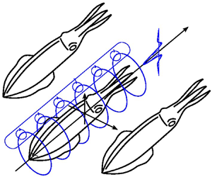
  $l$. This velocity field can be approximated as induced by a finite number of elementary vortex rings, each substituting for the bound vorticity over a small portion of the body (see figure 1a):
 \begin{equation} u = \varGamma \varUpsilon_{bound},\quad \textrm{where}\ \varUpsilon_{bound} = \sum_{j=1}^{n_r} \gamma_j\,\varUpsilon_{ring}(x-x_j,r), \end{equation}
where  $x_j = x_{nose} + (\,j-1/2) l/n_r$ is the position of the
  $j$th vortex ring, and
  $x_{nose}$ corresponds to the front point of the body. The circulation distribution coefficients
  $\gamma _j$ are calculated as follows. First, dimensional circulations
  $\varGamma _j$ are determined from a least mean square fit of the velocity profile along a line parallel to the axis and at a constant distance from it. Then
  $\varGamma$ is found by summing all vortex ring circulations
  $\varGamma _j$. Finally, the coefficients are evaluated as
  $\gamma _j = \varGamma _j/\varGamma$.

Figure 1. (a) Schematic representation of the vortex ring and momentumless wake model. Dimensional circulations  $\varGamma _j$ are related to the dimensionless coefficients
  $\gamma _j$ by
  $\varGamma _j = \gamma _j \varGamma$. (b) Postulated bound circulation distribution. (c) Postulated normalized radial profile of the momentumless wake axial velocity component. (d) Axial velocity component
  $u$ over the azimuthal symmetry plane, obtained using the far-field approximation. The black dashed line connects the points of minimum
  $u$ at every
  $d_{min}$ in the rear part of the field. The black dash-dotted line connects the points of minimum
  $u$ at every
  $d_{min}$ in the front part of the field.
The above approach can be regarded as a variant of the vortex lattice method, which substitutes the solid body in a potential flow by a perpendicular lattice of vortices. This approximation is also suitable for real flows if the boundary layers are thin and there is no flow separation. In the axisymmetric case, the longitudinal vortices have zero circulation. This leads us to the approximation of the body by a system of coaxial vortex rings. If we calculate the velocity at a test point so far from the body that the distances between the vortex rings are much less than the distance from the body to the test point, then it becomes possible to neglect the distance between the coaxial vortex rings, and associate all vorticity with only one vortex ring of radius  $a$ and circulation
  $\varGamma$.
2.2. Velocity field of a momentumless wake
An analytical solution of the incompressible Navier–Stokes equations that describes a steady laminar momentumless wake can be found in Korobko, Shashmin & Shul'man (Reference Korobko, Shashmin and Shul'man1986). However, that solution shows the velocity decay downstream as  $x^{-2}$, whereas turbulent momentumless wakes rather decay as
  $x^{-1.5}$ (Sirviente & Patel Reference Sirviente and Patel2000). Since there is no analytical solution for the mean flow velocity of the turbulent momentumless wake, let us modify the laminar functional relation (Korobko et al. Reference Korobko, Shashmin and Shul'man1986) to become consistent with the turbulent rate of decay. For this purpose, we introduce adjustable parameters
  $C$ and
  $p$. Also, we regularize the singularity at
  $x=0$. Thus the axial velocity component is given by
 \begin{equation} u = \varGamma \varUpsilon_{wake},\quad \varUpsilon_{wake} = \frac{C}{a}\,\xi\,\frac{1}{1+\xi^{2-2p}}\,g(\eta), \end{equation}
where it is postulated that the radial profile is a function of the similarity variable
 \begin{equation} \eta = \frac{r}{a}\,\frac{\xi^p}{Re^p}, \end{equation}
with  $\xi = x/a$, and the Reynolds number
  $Re = U_\infty a / \nu$ being based on
  $U_\infty$, the far-field velocity that is equal in magnitude to the swimming speed, and
  $\nu$, the kinematic viscosity of the fluid. Since this is a far-field approximation, the virtual wake origin is set at
  $x=0$. This simplification has little effect on the accuracy when
  $\xi \gg l/a$.
The radial profile of the velocity,  $g(\eta )$, depends on the spatial distribution of the momentum excess and deficit in the wake. We are interested particularly in the case of
  $g(\eta )$ changing sign twice (see Appendix B for more detail):
 \begin{equation} g(\eta) ={-} \left( 1 - \frac{\eta^2}{\eta_1^2} \right) \left( 1 - \frac{\eta^2}{\eta_2^2} \right) \exp\left({-\frac{\eta^2}{\eta_3^2}}\right), \end{equation}
where  $\eta _1$,
  $\eta _2$ and
  $\eta _3$ are constant parameters.
Since the wake is momentumless and axisymmetric, it is required that
 \begin{equation} \int_0^\infty 2 {\rm \pi}\eta\,g(\eta) \,\mathrm{d} \eta = 0. \end{equation}
It follows that only two of the three parameters can be adjusted freely, since
 \begin{equation} 2\,\frac{\eta_3^2}{\eta_1^2}\,\frac{\eta_3^2}{\eta_2^2} - \frac{\eta_3^2}{\eta_1^2} - \frac{\eta_3^2}{\eta_2^2} + 1 = 0. \end{equation}
The far-field approximation to the velocity due to both the bound vorticity and the momentumless wake is constructed as
 \begin{equation} u = \varGamma \varUpsilon,\quad \mathrm{where}\ \varUpsilon = \begin{cases} \varUpsilon_{bound} & \textrm{if}\ x < 0,\\ \varUpsilon_{bound} + \varUpsilon_{wake} & \textrm{otherwise}. \end{cases} \end{equation}
The postulate that the momentumless wake intensity scales linearly with the bound circulation  $\varGamma$ is justified as follows. The drag region of the wake is formed by the separated boundary layer, which carries the bound circulation. The jet region has momentum equal in magnitude but of opposite sign, to ensure that the total momentum vanishes. Therefore, the wake velocity must be proportional to
  $\varGamma$.
2.3. Condition of multiple swimmers propelling at the same velocity
Let us focus on a situation when  $N$ swimmers self-propel in a fluid otherwise at rest. All swim at the same speed
  $-U_0$ in the same direction, such that their relative positions do not vary. Hence, in the reference frame moving with the swimmers, the velocity field of the fluid is steady. The inflow velocity at the location of the
  $i$th swimmer is the superposition of
  $U_0$ and the velocity induced by all companion swimmers:
 \begin{equation} U_i = U_0 + \sum_{\substack{j=1\\ j \neq i}}^N{u_{ij}}, \end{equation}
where  $u_{ij}$ is the velocity induced by the
  $j$th swimmer at the location of the
  $i$th swimmer
  $\boldsymbol {x}_i$. These inflow locations are taken at the swimmer body centres, assuming that the induced velocity has little variation over the body length. Let us use the far-field approximation derived in the previous subsections,
 \begin{equation} u_{ij} = \varGamma_j\,\varUpsilon(\boldsymbol{x}_i), \end{equation}
where  $\varUpsilon (\boldsymbol {x}_i)$ is calculated as defined in (2.13).
The circulation  $\varGamma$ and the hydrodynamic power
  $P$ of a swimmer are functions of the local inflow velocity of the surrounding fluid
  $U$. These functions can be linearized for a small deviation of
  $U$ from the reference velocity
  $U_0$:
 \begin{gather} \varGamma(U) = \left. \varGamma \right|_{U_0} + \left.\frac{\partial \varGamma}{\partial U}\right|_{U_0} (U-U_0), \end{gather}
 \begin{gather}P(U) = \left. P \right|_{U_0} + \left.\frac{\partial P}{\partial U}\right|_{U_0} (U-U_0), \end{gather}
where  $\varGamma$,
  $P$ and their derivatives at
  $U_0$ are evaluated using computational fluid dynamics (CFD) simulations, as explained below. For a swimmer surrounded by neighbours, it is assumed that
  $U$ differs from
  $U_0$ by a small amount of induced velocity, warranted for the Taylor series approximation (2.16) and (2.17). Figure 1(d) confirms that
  $|u_{ij}|<0.02 U_0$ for
  $y>2a$. Substituting (2.14) and (2.15) into (2.16), we obtain
 \begin{equation} \varGamma_i = \left. \varGamma \right|_{U_0} + \left.\frac{\partial \varGamma}{\partial U}\right|_{U_0} \sum_{\substack{j=1\\ j \neq i}}^N{\varGamma_j\,\varUpsilon (\boldsymbol{x}_i)},\quad i = 1,\ldots,N. \end{equation}
When positions  $\boldsymbol {x}_1,\ldots,\boldsymbol {x}_N$ are fixed a priori, (2.18) constitutes a system of
  $N$ linear equations with
  $N$ unknowns
  $\varGamma _1,\ldots, \varGamma _N$. By solving this system and substituting the solution into (2.15), we evaluate the induced velocities
  $u_{ij}$ for all
  $i = 1,\ldots,N$ and
  $j = 1,\ldots,N$. Then the effective inflow velocities
  $U_i$ of each swimmer are evaluated using (2.14). Finally, using (2.17), we calculate the mechanical power expenditure of each swimmer as
 \begin{equation} P_i = \left. P \right|_{U_0} + \left.\frac{\partial P}{\partial U}\right|_{U_0} (U_i-U_0),\quad i = 1,\ldots,N. \end{equation}
2.4. Optimization objective
We aim to minimize the normalized school-average mechanical power expenditure,
 \begin{equation} \bar{P} = \frac{1}{\left. P \right|_{U_0} N} \sum_{i=1}^{N} P_i, \end{equation}
under the condition that all swimmers move in the same direction at the same constant speed  $U_0$. Minimization is achieved by finding the best relative position of the swimmers. Thus, without loss of generality, we assume
  $\boldsymbol {x}_1=\boldsymbol {0}$. The Cartesian scalar components of
  $\boldsymbol {x}_2,\ldots, \boldsymbol {x}_N$ provide
  $3N-3$ optimization parameters.
The far-field approximation fails in the vicinity of the swimmer. Therefore, only solutions with large enough spacing between the swimmers should be admitted as optimal. This is achieved by introducing a penalty function
 \begin{equation} V_p = \max \left\{0, A_p \left( 1 - \frac{d_{min}}{\sigma_p a} \right) \right\}, \end{equation}
where  $\sigma _p$ is a parameter that controls the minimum allowed distance between swimmers as a multiple of
  $a$, and
  $A_p \gg 1$ is a constant penalty parameter (we use
  $A_p = 10^4$).
The pairwise lateral separation distance between the swimmer centroids  $\boldsymbol {x}_i=(x_i,y_i,z_i)^{\rm T}$,
  $i=1,\ldots,N$, is calculated as
 \begin{equation} d_{min} = \min_{\substack{i = 1,\ldots,N\\ j = 1,\ldots,i-1}} \sqrt{(y_j-y_i)^2+(z_j-z_i)^2}. \end{equation}
The penalty function (2.21) ensures that the lateral separation between swimmers is no less than  $d_{min}$. The axial coordinate is not included in the formula, therefore the optimizer cannot choose to place swimmers either in the immediate proximity or in the wake. Thus we disallow placing swimmers at locations where the flow is vorticity-dominated (as known from the CFD data). The minimization objective function is
 \begin{equation} J = \bar{P} + V_p. \end{equation}
3. Results of the numerical optimization
3.1. Individual swimmer parameter fitting
The far-field interaction model requires knowledge of the velocity field of an isolated swimmer, as well as its hydrodynamic power expenditure. We derived representative values of the necessary parameters from CFD simulations of a real-scale streamlined-body artificial swimmer using the SIEMENS PLM software Simcenter STAR-CCM+ 2020.1. The CFD methodology is described in a precursor study by Li et al. (Reference Li, Duan, Godoy-Diana and Thiria2023), and the simulations used in this study are detailed in the Supplementary Information. The swimmer has body half-width  $a=0.175$ m and body length (
 $BL$)
$BL$)  $l=20a$. In all calculations, we place the origin of the attached coordinate system at a distance
  $9.4 a$ downstream from the nose. Thus the position of the tail in this coordinate system is
  $x_{tail}=10.6 a$. The swimmer cruise speed is
  $U_0=0.466\,BL\,{\rm s}^{-1}$. The numerical dimensional output data from the CFD simulations are converted in this section into dimensionless coefficients multiplied by proper scaling factors, for greater generality. Thus the hydrodynamic power at cruise is evaluated in STAR-CCM+ as
  $P |_{U_0}=0.107 \rho U_0^3 {\rm \pi}a^2$, where
  $\rho$ is the water density.
The total circulation  $\varGamma$ of the far-field vortex ring model was determined as follows. The CFD velocity was sampled at the grid points distributed on a line that was offset from the symmetry axis by
  $2.27a$. Then the far-field formula (2.7) was evaluated at the same points. The bound vorticity was approximated by
  $n_r=21$ rings. The products
  $G_j = \varGamma \gamma _j$ were treated as unknown coefficients, thus their values were found using the linear regression. The total circulation
  $\varGamma |_{U_0}=-16.5 U_0 a$ was found by the summation of
  $G_j$ over
  $j$ from 1 to
  $n_r$. Finally, the distribution coefficients
  $\gamma _j = G_j/\varGamma$ were determined; see figure 1(b).
Further, the momentumless wake model coefficients were fitted to the CFD data at  $U_0$. The corresponding Reynolds number was
  $Re = a U_0 / \nu = 2.8 \times 10^5$. The radial profile
  $g(\eta )$ was adjusted to the data at distance
  $3.26 a$ downstream from the tail. This resulted in the parameter values
  $\eta _1 = 2.15$,
  $\eta _2 = 5.5$,
  $\eta _3 = 3.34$, and a profile shown in figure 1(c). The parameter values
  $C=0.516$ and
  $p=-0.176$ ensure that the decay along the wake axis agrees with the CFD data. Figure 1(d) visualizes the velocity reconstructed from the far-field approximation.
The velocity field of the momentumless wake decays in the lateral direction  $r$ much faster (exponentially) than the velocity field of the vortex rings (that decays algebraically). Therefore, when the velocity is sampled on a line parallel to the axis, if the offset distance is sufficiently large for the far-field vortex ring approximation to be valid, then the momentumless wake contribution at that station is negligible. Likewise, on the axis behind the swimmer, the momentumless wake velocity decays more slowly with the downstream distance
  $x$ than the vortex-ring-induced velocity. Therefore, coefficients of the bound vorticity model and coefficients of the momentumless wake model can be determined independently.
Calculation of the derivatives  $(\partial \varGamma /\partial U) |_{U_0}$ and
  $(\partial P/\partial U) |_{U_0}$ required additional simulations at two slightly different speeds. These simulations used a coarser mesh. At
  $U_-=0.9U_0$, we obtained the circulation
  $\varGamma _-= -15.9 U_0 a$ and power
  $P_-= 0.079 \rho U_0^3 {\rm \pi}a^2$. At
  $U_+=1.1U_0$,
  $\varGamma _+= -19.4 U_0 a$ and
  $P_+= 0.140 \rho U_0^3 {\rm \pi}a^2$. These data enable finite-difference approximations to the derivatives,
  $(\partial \varGamma /\partial U) |_{U_0}= -17.4 a$ and
  $(\partial P/\partial U) |_{U_0}= 0.304 \rho U_0^2 {\rm \pi}a^2$.
3.2. Parameters of optimal schools
The optimization problem consists in finding the swimmer positions  $\boldsymbol {x}_2,\ldots, \boldsymbol {x}_N$ relative to the first swimmer such as to minimize the objective function (2.23). We use the CMA-ES genetic optimization algorithm (Hansen, Müller & Koumoutsakos Reference Hansen, Müller and Koumoutsakos2003). To accelerate the search, the swimmer coordinates vary with discrete increments that are multiples of
  $0.01a$, and the whole domain is a cube with side length
  $2Nl$. In all cases, the population size parameter was equal to 500, and a sufficient number of iterations were performed to ensure that the objective function does not change by more than
  $10^{-4}$ during the last 100 iterations.
Since  $u$ decays with the lateral spacing between the swimmers, an important control parameter is
  $\sigma _p$, which enters in the penalty function (2.21). All optimal formations that we found activated the constraint
  $d_{min}=\sigma _p a$. Figure 2(a) shows how the school average power
  $\bar {P}_{min}$ that corresponds to the minimized cost function
  $J_{min}$ varies with the minimum dimensionless separation distance between swimmers
  $d_{min}/a$, which is controlled by
  $\sigma _p$. The latter is an external control parameter. Its value may be selected, for example, from the accuracy considerations of the far-field approximation or from collision avoidance considerations. The relationship between
  $d_{min}/a$ and
  $\bar {P}_{min}$ suggests that reducing the lateral distance in a school can enhance energy-saving effects. Due to this,
  $d_{min}/a$ would tend to 0 under unrestricted
  $d_{min}/a$. In the context of optimization, the role of the penalty function is to impose constraints on the dimensionless lateral separation. It is necessary to impose such constraints on
  $d_{min}/a$ during the optimization process to avoid swimmer overlap and to match real-world situations. Energy savings of several per cent (relative to
  $P |_{U_0}$) may be realized at
  $d_{min}$ as small as
  $2a$ to
  $5a$. Greater lateral separation leads to vanishing energy saving. Trends for schools of different sizes are similar, but lower
  $\bar {P}_{min}$ of larger schools shows that they are slightly more efficient in saving energy. To elucidate the trend with
  $d_{min}/a$, figure 2(b) shows the power economy
  $1-\bar {P}_{min}$ on the logarithmic scale. It decays at a rate close to
  $-2$ for all
  $N$, and the power-law constant is larger for greater
  $N$.
$N$.

Figure 2. (a) School average power  $\bar {P}_{min}$ as a function of the minimum dimensionless lateral separation distance between swimmers,
  $d_{min}/a$, for four different school sizes
  $N$. Continuous lines correspond to the results of simultaneous optimization of the positions of
  $N-1$ swimmers. Markers correspond to the results obtained by sequentially adding one swimmer to the school and optimizing its position, shown for
  $d_{min}/a=2$,
  $3$ and
  $4$ as ‘
 $\circ$’, ‘
 $\times$’ and ‘
 $+$’ signs, respectively. (b) The quantity
  $1-\bar {P}_{min}$ shown as a function of
  $d_{min}/a$ on the logarithmic scale, for different school sizes
  $N$. The continuous lines show the optimization results, and the dashed lines are the linear regression lines on those data:
  $1-\bar {P}_{min}=0.220 (d_{min}/a)^{-1.97}$ for
  $N=2$,
  $1-\bar {P}_{min}=0.286 (d_{min}/a)^{-1.90}$ for
  $N=3$,
  $1-\bar {P}_{min}=0.354 (d_{min}/a)^{-1.82}$ for
  $N=7$, and
  $1-\bar {P}_{min}=0.392 (d_{min}/a)^{-1.83}$ for
  $N=11$. (c) Plots of
  $\bar {P}_{min}$ obtained using the sequential increment of
  $N$, as functions of
  $N$, for
  $d_{min}/a=3$,
  $4$ and
  $5$.
$5$.
Figure 3 shows an example of a typical optimal school. The frontal projections occupy a small region of the  $yz$ plane, such that the lateral distances between neighbours are almost as small as possible, i.e. about
  $5a$ (
 $0.25\,BL$). From the side view, each pair of neighbours forms a leader–follower pair with
  $11.4a$ (
 $0.57\,BL$) longitudinal offset. Incidentally, the best energy-saving formations of two tetra fish were previously found to have respective separation distances of about
  $0.35\,BL$ and
  $0.75\,BL$ (Li et al. Reference Li, Kolomenskiy, Liu, Thiria and Godoy-Diana2019), and the optimum was explained from the mean flow field considerations. It appears that similar effects apply to an elementary leader–follower pair in a school of axisymmetric swimmers. Note that any swimmer has at most two neighbours in its vicinity. Therefore, the induced velocities remain small.

Figure 3. Optimized schools of  $N=11$ individuals with
  $d_{min}/a=5$: (a) front view and (b) side view of a school obtained by numerical optimization; (c) front view and (d) side view of a school obtained by a direct-rule-based method. Individuals are labelled by numbers from 1 to 11.
3.3. Two- and three-swimmer optimal schools
The optimality of chain formation motivates us to revisit the groups of two and three swimmers. They can be considered as elementary blocks of larger schools, because the nearest neighbours interact most strongly, even if in our model they rely only on the far field such that unsteady effects are not included.
The minimal school consists of two swimmers ( $N=2$); see figure 4(a). The position of the second swimmer relative to the first swimmer is optimized. Without loss of generality, the first swimmer is located at the origin of the coordinate system, and the second swimmer is on the
  $xy$ plane. Thus only the distance
  $\rho$ and the polar angle
  $\theta$ are non-zero. The optimal values are shown in figure 5, as functions of the minimum dimensionless lateral separation distance
  $d_{min}/a$. Both quantities increase monotonically. This means that the optimally selected lateral separation increases at a greater rate than the longitudinal separation.

Figure 4. Geometrical parameters of (a) a two-swimmer school, and (b) a three-swimmer school. Points  $S_1$,
  $S_2$ and
  $S_3$ correspond to the first, second and third swimmers, respectively. The coordinate system
  $S_2 x'y'z'$ is obtained from
  $S_1 x y z$ by translation of the origin from the first swimmer to the second swimmer. The planes
  $S_2 x'y'$ and
  $S_1 x y$ coincide, because the
  $z$-coordinate of the second swimmer is zero. The angle
  $\theta _{lead}$ is between the negative semi-axis
  $S_1 x$ and the line that connects
  $S_1$ with
  $S_2$. Point
  $O''$ marks the perpendicular projection of the third swimmer on the
  $S_2 x'$ axis. Axis
  $O''y''$ is parallel to
  $S_2 y'$, and it resides on the
  $S_2 x'y'$ plane. Angle
  $\theta _{hind}$ is the angle between the negative semi-axis
  $S_2 x'$ and the line that connects
  $S_2$ with
  $S_3$. Angle
  $\phi _{hind}$ is the angle between the line
  $O'' S_3$ and the
  $O'' y''$ axis. Schematic side views: (c) a two-swimmer school; (d) a three-swimmer school. Respective top views: (e) a two-swimmer school; (f) a three-swimmer school. The minimum dimensionless lateral distance between neighbours is
  $d_{min}/a=3$.

Figure 5. Optimal values of the geometrical parameters of two- and three-swimmer schools: (a) dimensionless distance between neighbours; (b) elevation; (c) bank. The black dashed lines show the polar coordinates  $\rho$ and
  $\theta$ of the minimum (most negative) induced velocity in the rear part of the swimmer's field, and they correspond to the black dashed line in figure 1(d). The black dash-dotted lines show the polar coordinates
  $\rho$ and
  $-\theta$ of the minimum (most negative) induced velocity in the front part of the swimmer's field, and they correspond to the black dash-dotted line in figure 1(d).
As conjectured in § 1, the follower is optimally placed in the rear updraft region of the leader's induced flow: the blue circles in figures 5(a,b), which show the position of the follower relative to the swimmer, almost coincide with the black dashed lines that visualize the leader's induced field minimum velocity point coordinates as functions of relative separation distance  $d_{min}/a$. Importantly, this formation also minimizes the leader's energy cost, because the leader's position relative to the follower is in the front updraft region of the follower's induced flow: the blue circles are also very close to the black dash-dotted lines.
Similar staggered formations with lateral separation  $0.5 l$ and longitudinal offset
  $0.75 l$ were found to minimize the cost of transport of a pair of tetra fish (Li et al. Reference Li, Kolomenskiy, Liu, Thiria and Godoy-Diana2019). This arrangement corresponds to
  $d_{min}/a = 6$,
  $\rho /a = 10.8$,
  $\theta =34^\circ$ in polar coordinates. It was explained in Li et al. (Reference Li, Kolomenskiy, Liu, Thiria and Godoy-Diana2019) by the same mechanism of mean velocity updraft as considered in this study. However, in Li et al. (Reference Li, Kolomenskiy, Liu, Thiria and Godoy-Diana2019), the fish undulated laterally, and the amount of power economy varied with the phase difference between the leader and the follower. The greatest power economy would be achieved at the phase matching of the follower undulation with the incoming wave from the leader, such as that described by Li et al. (Reference Li, Nagy, Graving, Bak-Coleman, Xie and Couzin2020). Thus benefit from the far-field interaction and unsteady mechanisms can accumulate.
In a school of three swimmers ( $N=3$, figure 4b), the optimal configuration of the leading pair is close to that found in the two-swimmer case (
 $N=2$):
  $\rho _{lead}$ is slightly less and
  $\theta _{lead}$ is slightly larger than the respective values for
  $N=2$. The points fall on the rear updraft line. The position of the third swimmer relative to the second swimmer is given by three non-zero polar coordinates. The values
  $\rho _{hind}$ and
  $\theta _{hind}$ coincide with
  $\rho _{lead}$ and
  $\theta _{lead}$, respectively. The
  $\phi _{hind}$ angle is
  $120^\circ$. The two pairs are, essentially, two two-swimmer optimal formations combined and rotated such that the lateral separation distance between the first and the third swimmer equals
  $d_{min}$. Thus the follower in each pair maximizes the beneficial interaction with its leader, and the two pairs adjust their relative orientation to gain extra benefit.
3.4. Rules for large schools
The previous three-swimmer analysis motivates a direct-rule-based method for constructing larger energy-saving schools. The first three swimmers are placed such that  $\rho _{lead}$,
  $\theta _{lead}$,
  $\rho _{hind}$ and
  $\theta _{hind}$ are on the rear updraft line, as in figures 5(a,b) at the required
  $d_{min}$, and
  $\phi _{hind}=120^\circ$. The fourth swimmer is added behind the third one such that the second, third and fourth swimmers form a three-swimmer school obeying the same rule, but the
  $\phi$ angle is
  $-120^\circ$. Thus we ensure that the fourth swimmer is in the updraft of all those in front. The fifth swimmer is added with
  $\phi =120^\circ$, and so on. Figures 3(c,d) show a formation obtained for
  $N=11$, and the pattern extends intuitively to any large
  $N$.
$N$.
The results in figure 2(a) suggest that  $\bar {P}_{min}$ is smaller for larger schools. To estimate the lower bound of
  $\bar {P}_{min}$, for a given
  $d_{min}/a$, we use the above rules to construct schools with
  $N$ ranging from 3 to 100. The markers in figure 5 show that the schools obtained using this method are close to optimal. Visually, the values of
  $\bar {P}_{min}$ are indistinguishable from the
  $(3N-3)$-parameter numerical optimization results. The discrepancy is either positive or negative, which means that both algorithms may deliver slightly suboptimal results. Figure 2(c) displays
  $\bar {P}_{min}$ obtained using the direct-rule-based method, as a function of
  $N$. At
  $d_{min}/a=3$, increasing
  $N$ up to
  $100$ may provide energy benefit, but the far-field approximation may fail at this small
  $d_{min}/a$. For more trustworthy values
  $d_{min}/a=4$ and
  $5$, the optimization results show that schools of
  $N \approx 15$ swimmers are practically as energy-saving as the largest schools.
4. Concluding remarks
Our model suggests that self-propelled 3-D swimmers can exploit each other's induced far field such that the entire school acquires a considerable net energy benefit. This gain is smaller than in two dimensions, but it is non-negligible (several per cent) if the swimmers are not far away from each other ( $d_{min}/a \le 5$).
The optimal schools save energy by exploiting the following properties: (i)  $\partial P / \partial U$ of an isolated swimmer is positive (see Appendix A); (ii) the flow is slowed down everywhere upstream of the head of a swimmer, and everywhere downstream of the tail of a swimmer, except in the wake (see figure 1d); (iii) the total flow is constructed by superposition of individual swimmer flows in the regions exterior to the boundary layers and wakes. The first two properties make it possible to find an arrangement where every swimmer saves energy: arrange them in a chain so that they are all upstream (downstream) of each other's head (tail). The second and third properties make it so that increasing the number of swimmers will increase the energy savings. By adding another swimmer in a chain formation, all the other swimmers will feel an even slower flow, thereby increasing energy savings. However, the third property implies that the distances between the swimmers are large enough to ensure that the inflow velocities evaluated at their central points are representative of the average inflow velocity over the body.
The interactions based on the far-field interference are distinct from the vortex phase matching (Li et al. Reference Li, Nagy, Graving, Bak-Coleman, Xie and Couzin2020) and the leading-edge vortex enhancement (Seo & Mittal Reference Seo and Mittal2022) mechanisms of two fishes that swim near each other. The latter require kinematic adjustment of the follower's tail beat to harvest the leader's wake with the maximum efficiency. The far-field interaction mechanism, on the other hand, depends on the time-averaged velocity. It is weak if we consider only a pair of swimmers ( $N=2$). But the average per capita energy benefit increases considerably with the number of individuals in the school, up to
  $N \approx 15$.
Optimal formations found by the optimizer in this study are chain formations. This formation exists in fish and squid schools, although it is not the most typical one. Some further enhancement of the model may be necessary, but it is also possible that energy optimization is not always the main objective.
Our approach is in many respects similar to well-known low-Reynolds-number models. But while the velocity superposition is exact in the limit of small  $Re$, it is only a linearized approximate method in our situation. The predictive capacity of the model is limited further by the simplifications of using only one control point per individual, only the axial velocity component and the steady flow approximation. Therefore, the exact amounts of the energy benefit need to be verified further by e.g. Navier–Stokes simulations. But the model suggests clearly that individual swimmers within a school can occupy positions according to the perceived time-averaged velocity such that the school would expend less energy than the same number of isolated individuals swimming at the same speed over the same distance.
Acknowledgements
D.K. and J.S. thank the Bayreuth Humboldt Centre for the support of this project. Three anonymous reviewers are thanked for constructive comments and suggestions.
Funding
G.L. is funded by Japan Society for the Promotion of Science (JP20K14978).
Declaration of interests
The authors report no conflict of interest.
Appendix A. The CFD simulation on an individual swimmer
The CFD simulation on an individual swimmer has been introduced earlier in Li et al. (Reference Li, Duan, Godoy-Diana and Thiria2023). In this study, we have performed Reynolds-averaged Navier–Stokes simulations using commercial software Siemens Simcenter STAR-CCM+ 2020.1. The swimmer is an autonomous underwater vehicle with a propeller. Its body is axisymmetric, of 3.4 m length and 0.35 m diameter. The geometrical centre of the body is located 1.64 m downstream from the nose.
The CFD software and turbulence model were validated previously in a study focused on rotational wind blades (Fang et al. Reference Fang, Li, Duan, Han and Zhao2021). The propeller zone, which rotates, features the finest computational mesh, while the other parts are static regions covered by a Cartesian mesh. The static mesh is refined at the swimmer surface and rear zone. The boundary condition at the frontal surface of the computational domain is set as a velocity inlet at various values in each case. The rear surface of the computational domain is set as a zero-pressure outlet. The side surfaces are set as symmetry boundaries. The baseline parameters used in the simulations are listed in table 1.
Table 1. Parameters of baseline individual swimmer simulations.

A cruising propeller rotational speed 320 rpm was established based on realistic data. Through multiple iterative simulations, the equilibrium condition (swimmer's drag equal to thrust) at cruising speed  $U_0 = 1.63\,{\rm m}\,{\rm s}^{-1}$ was determined. At this cruising speed, the propeller power and the flow field around the swimmer were recorded. Additionally, further simulations were conducted to compute the derivatives of power and flow field with respect to the cruising speed
  $U_0$. Using the same mesh, multiple simulations were implemented to approach the equilibrium condition at speeds of 90 %, 98 %, 102 % and 110 % of the cruising speed
  $U_0$. The results are presented in table 2.
Table 2. Computational results of individual swimmer performance.

To validate the mesh resolution and obtain detailed information about the wake field, an additional simulation with refined wake-zone mesh was implemented (parameters shown in table 3). Though the wake-zone mesh resolution in the additional simulation is several times higher than that of the baseline simulations, the extra refinement of the mesh does not bring any significant influence in the swimmer propulsive performance at the cruising speed (table 4), suggesting that the baseline mesh resolution was already sufficient to predict the propulsive performance. The detailed wake information obtained by this additional simulation was input into our theoretical model to describe the wake structure.
Table 3. Parameters of swimmer simulations using a fine mesh.

Table 4. Comparison between computational results using two different meshes.

The power expenditure curve is obtained from CFD simulations of an isolated swimmer. We performed a series of simulations at different speeds. The results are shown in figure 6. The power  $P$ increases nonlinearly with the swimming speed
  $U$. However, in the neighbourhood of
  $U_0$, this nonlinear dependence can be approximated by a linear dependence, following the usual procedure of linearization.

Figure 6. Power expenditure as a function of swimming speed. The speed is normalized by  $U_0$, and the power is normalized by
  $P_0 = P |_{U_0}$. Asterisk markers correspond to the values obtained from the CFD simulations. The blue dashed line is a power-law fit
  $P/P_0 = (U/U_0)^{2.7947}$. The red solid line is the linear fit used in the text. Over the interval
  $U/U_0 \in [0.9,1.1]$, the discrepancy is less than 3 %.
Appendix B. Wake velocity profile fitting
The velocity profile in Korobko et al. (Reference Korobko, Shashmin and Shul'man1986) consists of one jet region (excess velocity in the inner part of the profile) and one wake region (velocity deficit in the outer part due to the boundary layer separated from the swimmer's body). However, in our CFD simulation, the jet is produced by a propeller that has a central body, and the central body produces drag (velocity deficit). Then the propeller blades produce an annular jet (excess velocity). Finally, in the outer region, there is still a velocity deficit region due to the separated boundary layer. In order to have these three regions in the velocity profile, we introduces a simple (perhaps the simplest possible) modification of Korobko's formula. Note that while Korobko's formula is an exact result for a laminar momentumless wake, our intent is to have a semi-empirical formula suitable for the turbulent wake in our particular situation. Figure 7 displays a comparison between the fit and raw CFD data. The staircase in the CFD data is due to the low order of interpolation on the non-uniform grid.

Figure 7. Velocity excess/deficit in the wake. Dashed lines show the CFD results, and solid lines show the far-field approximation.
Figure 8 displays the CFD output data and the algebraic fit of the velocity sampled along the axis of the wake. The vertical line is drawn at the axial position  $x_{flex}$ where the line has an inflection point. This location is used for determining the fitting coefficients. In the central part of the CFD curve, the fit is very close to the CFD data, therefore choosing any
  $x$ in that region for measuring velocities does not affect the results of fitting.

Figure 8. CFD output data and algebraic fit of the velocity on the axis of the wake. The vertical line corresponds to the axial position  $x_{flex}$ where the line has an inflection point.
Appendix C. Vortex ring fitting
Figure 9 shows the results of a sensitivity analysis, when the velocity profiles are fitted on a lines at different distances from the swimmer axis. The results in the main text are obtained using the distance  $r_s^* = 4.36 a$, while figure 9 shows
  $\gamma _j$ and
  $\varGamma$ calculated using several smaller or larger values of the distance. When the distance
  $r_s$ is small, the far-field approximation fails, and the fitting is inaccurate. This happens at
  $r_s = 0.6 r_s^*$. When the distance
  $r_s$ is large, the distance between the
  $j$th and
  $(\,j+1)$th vortex rings is much smaller than
  $r_s$. In this situation, the entire system of vortex rings induces the velocity closely matching a single vortex ring with the circulation
  $\varGamma$. For that reason, the linear regression matrix becomes ill-conditioned; small numerical errors in the velocity sampling amplify, and lead to spurious dispersive error in the distribution of
  $\gamma _j$. In the intermediate range
 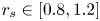 $r_s \in [0.8,1.2]$, the above-mentioned sources of error vanish, the results are not sensitive to
  $r_s$, and this is the correct fit.

Figure 9. Sensitivity of (a) the vortex ring circulation coefficients  $\gamma _j$, and (b) total circulation
  $\varGamma$, on the distance
  $r_s$ from the axis to the fitting line.
The results in figure 9 were obtained using  $n_r=21$ vortex rings. Smaller values of
  $n_r$ deteriorate the approximation accuracy at distances of the same order of magnitude as the vortex ring spacing or less. Increasing
  $n_r$ at a constant
  $r_s$ provokes the spurious dispersive error as discussed above. We found that the value
  $n_r=21$ is well adapted for the parameters of our CFD data set.


 Open access