


1. Introduction
Steady approaching flow past multiple circular cylinders has been the topic of many investigations due to its rich physics and relevance to engineering applications such as risers used to transport oil and gas products in offshore engineering. The flow past two cylinders in a side-by-side arrangement is one of the simplest configurations of flow around multiple cylinders and has been the focus of many studies in the literature. The flow features around two side-by-side cylinders are governed by gap-to-diameter ratio,  $g^* = G/D$, and Reynolds number
  ${\textit {Re}} = U_\infty D/\nu$, where
  $U_\infty$ is the incoming flow velocity,
  $G$ is the surface-to-surface distance,
  $D$ is the cylinder diameter and
  $\nu$ is the kinematic viscosity of the fluid.
The existing studies on this topic were mainly focused on flow features in the wake and corresponding hydrodynamic forces on the cylinders (e.g. Sumner et al. Reference Sumner, Wong, Price and Paï Doussis1999; Zhou & Mahbub Alam Reference Zhou and Mahbub Alam2016). Rich physics arising from the interaction of wakes behind the cylinders have been revealed at relatively low  ${\textit {Re}}$ (
 ${<\sim }160$) values through stability analysis and direct numerical simulations (DNS); see, e.g. Kang (Reference Kang2003); Carini, Giannetti & Auteri (Reference Carini, Giannetti and Auteri2014); Ren et al. (Reference Ren, Cheng, Xiong, Tong and Chen2021a). It was found that the flow at low
  ${\textit {Re}}$ undergoes transitions from a single bluff-body wake, via a flip-flop (FF) wake, to coupled-individual wakes such as in-phase (IP) and anti-phase (AP) flows with increasing
  $g^*$. Other flow modes such as asymmetric single bluff-body vortex shedding flows and bistable flows are also found over the above parameter space (Ren et al. Reference Ren, Cheng, Xiong, Tong and Chen2021a). It is noteworthy that most of those studies are limited to low
  ${\textit {Re}}$, where the flow was assumed to be two dimensional. There has not been any systematic study on three-dimensional (3-D) transitions for steady approaching flow around two side-by-side circular cylinders, to the best of the authors knowledge. It is unclear when the flow becomes 3-D flow and how the three-dimensionality affects the flow regimes identified in the two-dimensional (2-D) studies. We believe that the flow is three dimensional over parts of the parameter space (
 $g^*<2.5$ and
  ${\textit {Re}}<160$) covered by the published work. The first objective of the present study is to answer the above questions.
The wake states of steady flow past a fixed circular cylinder exhibits distinctive transitional features with increasing  ${\textit {Re}}$. The 2-D Kármán vortex street, which occurs at
  ${\textit {Re}} \sim 47$, becomes unstable to 3-D perturbations through a subcritical (i.e. hysteresis) transition at
  ${\textit {Re}}_{cr-1} \approx 189$. The mode A flow, featured by a regular 3-D structure with a spanwise wavelength
  $\lambda$ of approximately
  $4D$, occurs in the vicinity of
  ${\textit {Re}} > 189$. The pure mode A flow exists over a narrow range of
  ${\textit {Re}}$ before spanwise dislocations occur, i.e. mode
  ${\rm A}^*$. At
  ${\textit {Re}} \approx 230\unicode{x2013}260$, a gradual transition from mode
  ${\rm A}^*$ to mode B is observed. Mode B, which manifests strong growth of 3-D perturbation in the braids and between the forming vortices, becomes a dominant structure through a supercritical transition (i.e. non-hysteresis). Stability analysis predicts mode B to be unstable at
  ${\textit {Re}}_{cr-2} \approx 260$ (Barkley & Henderson Reference Barkley and Henderson1996), while experimental and numerical studies both observed a mode B structure at
  ${\textit {Re}} > \sim 230$ (Thompson, Hourigan & Sheridan Reference Thompson, Hourigan and Sheridan1996; Williamson Reference Williamson1996a). Mode B has a much shorter
  $\lambda$ of around
  $0.8D$. It has been demonstrated that mode A primarily originated from an elliptical instability of primary vortex cores, while mode B is associated with a hyperbolic instability of braid shear layers (e.g. Williamson Reference Williamson1996a; Thompson, Leweke & Williamson Reference Thompson, Leweke and Williamson2001). A third mode, known as a quasi-periodic (QP) mode, was discovered through stability analysis when
  ${\textit {Re}}$ exceeds approximately
  $377$ (Blackburn, Marques & Lopez Reference Blackburn, Marques and Lopez2005). The QP mode, however, has not been found in experimental studies likely due to the presence and dominance of the mode B flow (Leontini, Lo Jacono & Thompson Reference Leontini, Lo Jacono and Thompson2015).
Apart from the above three 3-D instability modes identified in the wake behind a single circular cylinder, a subharmonic mode C has been observed in various bluff-body flows. The mode C flow can be triggered under the following conditions:
(i) asymmetric geometry (e.g. Sheard, Fitzgerald & Ryan Reference Sheard, Fitzgerald and Ryan2009; Blackburn & Sheard Reference Blackburn and Sheard2010; Jiang & Cheng Reference Jiang and Cheng2020; Gupta et al. Reference Gupta, Zhao, Sharma, Agrawal, Hourigan and Thompson2023);
(ii) asymmetric incoming flow (e.g. Park & Yang Reference Park and Yang2018; Wang et al. Reference Wang, Zhu, Bao, Zhou, Ping, Han and Xu2019);
(iii) structural movement, e.g. a rotated cylinder (Rao et al. Reference Rao, Leontini, Thompson and Hourigan2013) and a transversely oscillated cylinder (Leontini, Thompson & Hourigan Reference Leontini, Thompson and Hourigan2007);
(iv) asymmetric wake, e.g. flow past a torus (Sheard, Thompson & Hourigan Reference Sheard, Thompson and Hourigan2003) and steady flow past four square cylinders (Zhang et al. Reference Zhang, Wang, Chen, Bao, Han, Zhou, Ping, Fu and Zhao2020).
Mode C is featured by fluctuations of spanwise structures with a period that is twice the vortex shedding period in the plane perpendicular to the cylinder axis. Rao et al. (Reference Rao, Leontini, Thompson and Hourigan2013) found that mode C becomes possible once the wake breaks its spatio-temporal symmetry, due to the presence of a local acceleration of the flow only on one side of the body. It has been demonstrated that the transition to mode C can be either supercritical or subcritical.
The second objective of the present study is to investigate the influence of wake interactions on the transition processes from 2-D to 3-D flows of the two side-by-side cylinders. We are particularly interested in the influences of asymmetric wake and FF wakes on the development of 3-D modes. We anticipate that the rich wake interactions have significant impact on the transition process and 3-D instability modes, given the subcritical nature of the 2-D to 3-D transition for an isolated cylinder.
The remainder of the paper is organised in the following manner. The numerical methods are introduced in § 2, followed by thorough mesh and numerical scheme validations in § 3. The characteristics of 2-D flows and 3-D wake transitions are presented in §§ 4 and 5, respectively. Discussions on the salient wake interactions in ASS and FF flows, the existence of other 3-D modes and flow regime classification based on 2-D and 3-D simulations are given in § 6. Finally, major conclusions are drawn in § 7.
2. Methodology
2.1. Two-dimensional DNS
The 2-D simulations are carried out to generate the base flow for the Floquet and 3-D DNS analyses. The following dimensionless incompressible Navier–Stokes (N–S) equations are solved numerically in the 2-D simulations:
 \begin{equation} \left.\begin{gathered} \boldsymbol{\nabla}\boldsymbol{\cdot}\boldsymbol{u}=0;\\ \partial\boldsymbol{u}/{\partial t}={-}(\boldsymbol{u}\boldsymbol{\cdot}\boldsymbol{\nabla})\boldsymbol{u}-{\boldsymbol{\nabla}}p+ {\textit{Re}}^{{-}1}\nabla^2\boldsymbol{u}. \end{gathered}\right\} \end{equation}
Here  ${\boldsymbol {u}} = (u, v)$ is the velocity vector corresponding to
  ${\boldsymbol {x}} = (x, y)$ in the Cartesian coordinates as shown in figure 1,
  $t$ is the time and
  $p$ is the pressure.
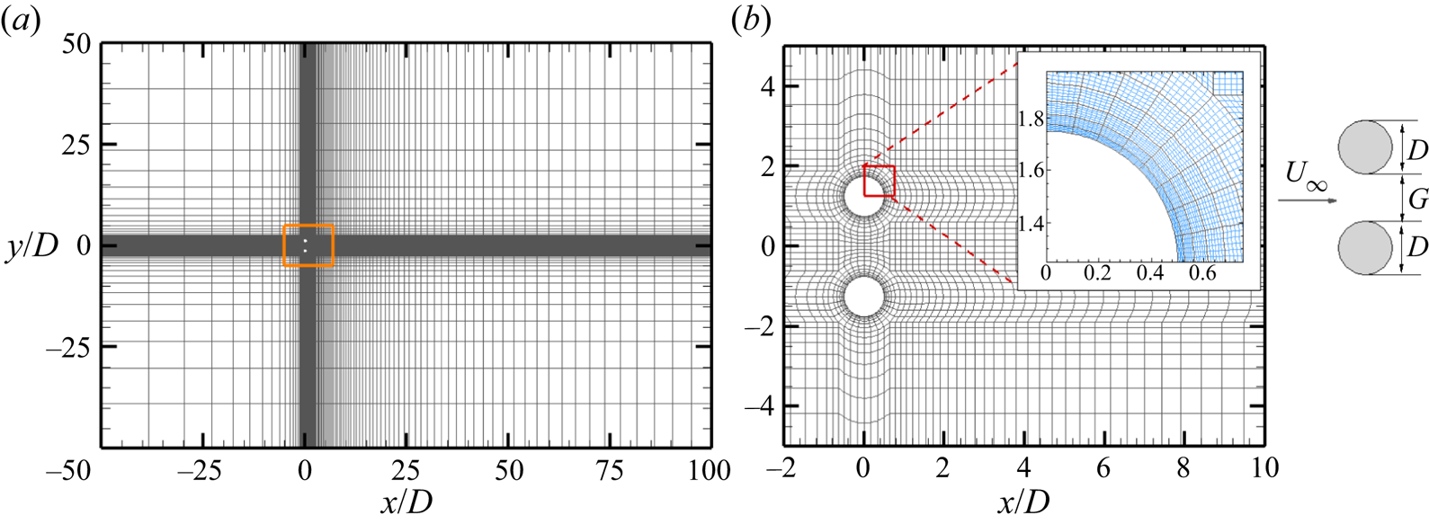
Figure 1. The  $h$-type mesh distributions of (a) the overall domain and (b) around the cylinders for two side-by-side cylinders at
  $g^* = 1.5$ used in the spectral/
 $hp$ element method. The total
  $h$-type macro-element number (
 $N_{el}$) is 6256. Each
  $h$-type mesh contains
  $N_p^2$ quadrature points. A close-up view on a
  $hp$-refined mesh consisting of sixth-order Lagrange polynomials (
 $N_p =6$) on Gauss–Lobatto–Legendre quadrature points is shown in the inset in (b), where the
  $p$-type mesh is in blue.
Equation (2.1) is solved using a spectral/hp element method embedded in Nektar++ (Cantwell et al. Reference Cantwell2015). For 2-D flow calculations, the velocity conditions of inlet and side boundaries are prescribed with a uniform velocity ( $u = U_\infty$ and
  $v = 0$). The Neumann boundary condition (
 $ {\partial } \boldsymbol {u}/ {\partial } \boldsymbol {n} = \boldsymbol {0}$) is implemented on the outlet boundary. A non-slip boundary condition (
 $\boldsymbol {u} = \boldsymbol {0}$) is enforced on the cylinder surfaces. A high-order Neumann pressure condition is specified on all domain boundaries except for a reference zero Dirichlet pressure condition on the outlet boundary. The spatial domain is discretised into quadrilateral finite elements and within each element both the geometry and fluid quantities are represented by
  $N_p$th polynomial expansions. A second-order time integration method, a velocity correction scheme and a Galerkin formulation are employed for all 2-D base flow simulations, which have been widely used and validated in the similar studies (Barkley & Henderson Reference Barkley and Henderson1996; Carmo et al. Reference Carmo, Sherwin, Bearman and Willden2008; Ren et al. Reference Ren, Cheng, Tong, Xiong and Chen2019, Reference Ren, Lu, Cheng and Chen2021b).
2.2. Floquet stability analysis
The Floquet analysis is performed on the same 2-D mesh to investigate the 3-D stability of the 2-D base flows. The growth of perturbation fields to the leading orders is governed by the linearised N–S equations
 \begin{equation} \left.\begin{gathered} \boldsymbol{\nabla}\boldsymbol{\cdot}\boldsymbol{u}'=0; \\ \partial\boldsymbol{u}'/{\partial t}={-}(\boldsymbol{U}\boldsymbol{\cdot}\boldsymbol{\nabla}\boldsymbol{u}'+ \boldsymbol{u}'\boldsymbol{\cdot}\boldsymbol{\nabla}\boldsymbol{U}) -{\boldsymbol{\nabla}}p'+Re^{{-}1}\nabla^2\boldsymbol{u}', \end{gathered}\right\} \end{equation}
where  $\boldsymbol {U}$ is the
  $T$-periodic base flow velocity fields,
  $\boldsymbol {u'}$ and
  $p'$ are the infinitesimal 3-D velocity and pressure perturbation fields.
Considering the system is homogeneous in the  $z$ direction, general perturbations to the velocity fields can be expressed as
 \begin{equation} \left.\begin{gathered} \boldsymbol{u}'(x,y,z,t) = \int_{-\infty}^{\infty} \hat{\boldsymbol{u}}(x, y, \beta, t)\,{\rm e}^{{\rm i}\beta z}\,\mathrm{d} \beta, \\ p'(x,y,z,t) = \int_{-\infty}^{\infty} \hat{p}(x, y, \beta, t)\,{\rm e}^{{\rm i}\beta z}\,\mathrm{d} \beta, \end{gathered}\right\}\end{equation}
where  $\beta$ is the spanwise wavenumber with corresponding wavelength of
  $\lambda = 2{\rm \pi} /\beta$. For the linearised N–S equations (2.2), modes with different
  $\beta$ do not couple. The perturbed fields
  $\hat {\boldsymbol {u}} = (\hat {u}, \hat {v}, \hat {w})$ and
  $\hat {p}$ depend only on
  $x$,
$x$,  $y$ and
  $t$. Following Barkley & Henderson (Reference Barkley and Henderson1996), the perturbation fields at a specific
  $\beta$ number can be written as
 \begin{equation} \left.\begin{gathered} \boldsymbol{u}'(x, y, z, t) = (\hat{u}\cos\beta z, \hat{v}\cos\beta z, \hat{w}\sin \beta z);\\ p'(x, y, z, t) = \hat{p}\cos\beta z. \end{gathered}\right\} \end{equation}
The full 3-D stability problem at given  ${\textit {Re}}$ can be reduced to a group of 2-D stability problems.
The Floquet analysis is performed by solving the growth of 2-D perturbation fields of a given  $\beta$ from one period to the next as
 \begin{equation} \hat{\boldsymbol{u}}(x, y, t+T)=\hat{\boldsymbol{u}}(x, y, t)\exp(\sigma T), \end{equation}
where  $T$ is the period of the base flow,
  $\mu = \exp (\sigma T)$ is termed as the Floquet multiplier and
  $\sigma$ is the Floquet exponent. A similar expansion is followed for
  $\hat {p}$. The Floquet multiplier for each
  $\beta$ can be obtained individually via Arnoldi iterations on a Krylov subspace. The base flow
  $\boldsymbol {U}$ is deemed as unstable to 3-D perturbations if
  $|\mu |$ crosses the unit circle (
 $|\mu | >1$), indicating the perturbations will grow exponentially with time. In contrast, the 2-D base flow is considered as stable if
  $|\mu | <1$, suggesting the 3-D perturbation will decay exponentially. This approach has been well described in the literature (Barkley & Henderson Reference Barkley and Henderson1996; Rao et al. Reference Rao, Leontini, Thompson and Hourigan2013; Leontini et al. Reference Leontini, Lo Jacono and Thompson2015).
The above procedure is achieved numerically through the following steps. Firstly, the 2-D DNS was carried out for at least 2000 non-dimensional time units ( $t^*=Ut/D$) to obtain fully developed flows for a considered case. The last 500 non-dimensional time units were used to track the time interval
  $\Delta T_i$ between two adjacent crests of the lift coefficient on the top cylinder (
 $C_{L-1}$). If the ratio between the standard deviation and the mean value of
  $\Delta T_i$ was less than 1 %, the flow was considered to have reached a fully developed state. A temporal Fourier interpolation is adopted to reconstruct the periodic base flow using
  $N_{t,s} = 32$ equi-spaced time slices over
  $T$. Secondly, the perturbation field
  $\boldsymbol {u}'$ was initialised by random noise, and then both base flow and the perturbation field were integrated forward in time. The spatial discretisation and time integration schemes are the same as those employed in 2-D DNS. The velocity boundary conditions of
  $\boldsymbol {u}' =\boldsymbol {0}$ and
  $\partial \boldsymbol {u}'/\partial \boldsymbol {n} =\boldsymbol {0}$ are imposed on the boundaries where the respective Dirichlet and Neumann boundary conditions were specified for the 2-D base flow calculations. In this way, the perturbed flow of
  $\boldsymbol {U}+\boldsymbol {u}'$ satisfies the same boundary conditions as the base flow
  $\boldsymbol {U}$ (Barkley & Henderson Reference Barkley and Henderson1996). Thirdly, the leading Floquet multipliers
  $\mu$ and corresponding modes are found by mapping the perturbation fields from one period to the next. This is achieved by employing the Arnoldi decomposition over the
  $K_n = 16$ dimension Krylov subspace. Calculations were carried out until the residual of the largest eigenvalue was less than
  $10^{-6}$ or after 800 iterations. Floquet analysis is employed over one
  $T$ due to the periodicity of the base flow. The selections of
  $N_{t,s} = 32$ and
  $K_n = 16$ were referred to the validation given by Carmo et al. (Reference Carmo, Sherwin, Bearman and Willden2008) and Ren et al. (Reference Ren, Cheng, Xiong, Tong and Chen2021a).
2.3. Three-dimensional DNS
A quasi-3-D approach, also known as the Fourier-spectral/hp element approach, is employed in 3-D DNS. In this approach the spectral/hp element is used in the cross-sectional plane and the Fourier discretisation is implemented in the  $z$ direction to resolve the full 3-D features of the flow. The solution of the velocity and pressure fields can be expressed through
  $M=N_z/2$ Fourier modes in the spanwise direction, where
  $N_z$ is the quadrature points of the
  $z$-direction expansion basis. Each
  $k$th Fourier mode, where
  $k=0,1,2,\ldots, M-1$, corresponds to the 3-D structure with a wavenumber of
  $\beta =2{\rm \pi} k/L_z$, where
  $L_z$ is the dimensionless spanwise length. Hence, the domain for the quasi-3-D simulation consists of 2-D discretisations repeated in the spanwise direction, allowing the 2-D mesh to be reused. Linear operators are applied to each component separately, and a coupling algorithm is employed to solve the nonlinear part when solving the N–S equations (Bolis Reference Bolis2013). This approach has advantages in terms of efficiency and it facilitates the parallelisation of the algorithms (Carmo et al. Reference Carmo, Sherwin, Bearman and Willden2008; Bolis Reference Bolis2013; Cantwell et al. Reference Cantwell2015; Xiong et al. Reference Xiong, Cheng, Tong and An2018).
In the simulation, sixth-order Lagrange polynomials ( $N_p = 6$) are used on Gauss–Lobatto–Legendre quadrature points. The
  $L_z$ for the 3-D simulation varies from
  $12$ to
  $28$, depending on
  $g^*$ and
  ${\textit {Re}}$ values. The large value of
  $L_z$ used herein is to make sure at least three pairs of 3-D structures can be resolved at low
  ${\textit {Re}}$. The employed Fourier modes are fixed at
  $M = 64$. Starting from a fully developed 2-D flow, each quasi-3-D simulation is conducted for at least 1000 non-dimensional time units to make sure the flow reaches a saturated state.
In order to identify the development of three-dimensionality in the near wake, the dimensionless enstrophies in the  $x$,
$x$,  $y$ and
  $z$ directions were recorded by integrating the vorticities over a volume of interest. The vorticities in three directions are defined as
 \begin{equation} \begin{cases} \omega_x = \partial w /\partial y - \partial v /\partial z, \\ \omega_y = \partial u /\partial z - \partial w /\partial x, \\ \omega_z = \partial v /\partial x - \partial u /\partial y. \end{cases} \end{equation}
The transverse enstrophy  $\varepsilon _{xy}$ and total enstrophy
  $\varepsilon _t$ are recorded during the simulation based on the formula
 $$\begin{gather} \varepsilon_{xy} = \frac{D^2}{2U^2 \varOmega} \int_{\varOmega} (\omega_x^2 +\omega_y^2)\,\mathrm{d}\varOmega, \end{gather}$$
 $$\begin{gather}\varepsilon_{t} = \frac{D^2}{2U^2 \varOmega} \int_{\varOmega} (\omega_x^2 +\omega_y^2+\omega_z^2)\,\mathrm{d}\varOmega, \end{gather}$$
where  $\varOmega$ is the integration volume at
  $x/D \in [0, 10 ]$,
  $y/D \in [-5, 5]$ and
  $z/D \in [0, L_z]$. The selection of this integration volume is because the near wake region constitutes the majority region where coherent structures are concentrated. The enstrophies were recorded every 10 non-dimensional time steps. The ratio of
  $\varepsilon _{xy}/\varepsilon _t$ is used in this study to represent the three-dimensionality in the near wake region as suggested by Papaioannou et al. (Reference Papaioannou, Yue, Triantafyllou and Karniadakis2006), since
  $\varepsilon _{xy}= 0$ for 2-D flow.
3. Numerical validations
3.1. Mesh convergence check
The selections of computational domain, mesh resolution and polynomial order  $N_p$ are based on Ren et al. (Reference Ren, Cheng, Xiong, Tong and Chen2021a). The mesh distribution near the cylinders and the computational domain are shown in figure 1, where the origin of the Cartesian coordinate system
  $(x, y)$ is placed at the centre of the gap. The total number of macro-elements (
 $N_{el}$) varies from 5731 to 6968, depending on
  $g^*$. The meshes for different
  ${\textit {Re}}$ with a fixed
  $g^*$ are identical. The non-dimensional time step
  $\Delta t$ is varied from 0.005 to 0.001 with increasing
  ${\textit {Re}}$. Other parameters governing the mesh set-up are detailed in Ren et al. (Reference Ren, Cheng, Xiong, Tong and Chen2021a). In most of the simulations in acquiring the base flow for Floquet analysis, zero velocity and pressure fields are employed as initial conditions (ICs), except for those cases in the bistable IP/FF and bistable IP/AP regions where the wake can assume one of the bistable states, depending on the ICs. The FF and AP states in those two bistable regions are generated through zero ICs (IC-0). In contrast, the IP flow is generated by using the IP flow (IC-IP) at upper/lower
  ${\textit {Re}}$ values and gradually descending/ascending
  ${\textit {Re}}$ values, respectively, during the simulation to reach the IP flow at targeted
  ${\textit {Re}}$.
Since the largest  ${\textit {Re}}$ considered in this study is 400 for the AP flow to capture the onset of the secondary 3-D mode (mode B) at
  $g^*=1.5$, additional
  $N_p$ convergence checks are performed at
  $g^*= 1.5$ and
  ${\textit {Re}}= 400$ by changing the
  $N_p$ from 5 to 8. The results in table 1, which are obtained over the last
  $500$ non-dimensional time units, indicate that the maximum relative differences of the root-mean-square lift coefficient
  $C_{L-1}'$ and the vortex shedding period
  $T_v$ based on
  $N_p = 6$ in case 1 differ by less than 0.4 % from other cases. We consider such small differences are acceptable and
  $N_p = 6$ is adequate for the purpose of the present study.
Table 1. Influence of the polynomial order ( $N_p$) on the root-mean-square lift coefficient
  $C_{L-1}'$ and vortex shedding period
  $T_v$ of side-by-side cylinders at
  $g^* = 1.5$ and
  ${\textit {Re}} = 400$. Here
  $\Delta t$ is the dimensionless time step. The values in the brackets behind
  $T_v$ and
  $C_{L-1}'$ are the relative errors compared with the reference case.

3.2. Validation of Floquet analysis: 3-D modes of a single cylinder
To ascertain the accuracy of the present study, Floquet analyses are benchmarked against results reported by Carmo, Meneghini & Sherwin (Reference Carmo, Meneghini and Sherwin2010), Barkley & Henderson (Reference Barkley and Henderson1996) and Blackburn et al. (Reference Blackburn, Marques and Lopez2005) for steady flow past an isolated circular cylinder at  ${\textit {Re}} = 180\unicode{x2013} 380$. The modulus of Floquet multipliers
  $|\mu |$ varying with
  $\beta$ for
  ${\textit {Re}} = 200\unicode{x2013} 350$ are shown in figure 2(a).
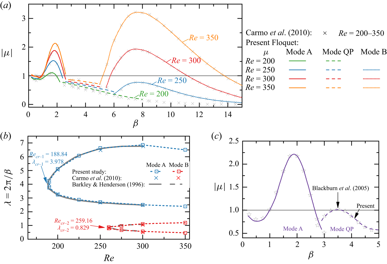
Figure 2. Floquet analysis of the steady flow past an isolated circular cylinder. (a) Evolutions of the modulus of Floquet multipliers  $|\mu |$ varying with the spanwise wavenumber
  $\beta$ for
  $Re = 200-350$. (b) Neutral stability curves plotted in the
  ${\textit {Re}}$ and wavelength (
 $\lambda = 2{\rm \pi} /\beta$) space. The curves in grey in (b) are reproduced from Barkley & Henderson (Reference Barkley and Henderson1996). The crosses in (b) represent the neutral points from Carmo et al. (Reference Carmo, Meneghini and Sherwin2010). (c)
  $|\mu | - \beta$ curve at
  ${\textit {Re}} = 380$ with a small outflow length of
  $20D$.
The two unstable regions of the  $\beta - |\mu |$ curves with real and positive
  $\mu$ correspond to the well-known mode A at small
  $\beta$ and mode B at large
  $\beta$, respectively. The regions of unstable Floquet modes (
 $|\mu |\ge 1$) are presented in the
  $\lambda (= 2{\rm \pi} /\beta ) - {\textit {Re}}$ space in figure 2(b), where discrete hollow squares denote the neutral
  $\lambda - Re$ curve where
  $|\mu |=1$ in figure 2(a). In this study the acronyms of
  ${\textit {Re}}_{cr-X}$/
 $\lambda _{cr-X}$ are used to indicate the critical
  ${\textit {Re}}$ and spanwise wavelength
  $\lambda$ for the onset of an ‘
 $X$-type’ 3-D mode. The critical values of an isolated circular cylinder, which are fitted using modified Bezier curves based on those hollow blue and red squares, are
  ${\textit {Re}}_{cr-A} \approx 188.84$ and
  $\lambda _{cr-A} \approx 3.978$ and
  ${\textit {Re}}_{cr-B} \approx 259.16$ and
  $\lambda _{cr-B} \approx 0.829$, respectively. Those values are consistent with the results reported by Barkley & Henderson (Reference Barkley and Henderson1996) (
 ${\textit {Re}}_{cr-A} = 188.5 \pm 1.0$ and
  $\lambda _{cr-A} = 3.96 \pm 0.02$,
  ${\textit {Re}}_{cr-B} = 259.0 \pm 2.0$ and
  $\lambda _{cr-B} = 0.822 \pm 0.007$).
To facilitate subsequent classification of the unstable 3-D modes for side-by-side cylinders, characteristics of mode A and mode B of an isolated cylinder are reviewed with reference to the existing knowledge through two typical cases at  $(Re, \beta ) = (200, 1.6)$ and (300, 7.0) in figures 3(a) and 3(b), respectively. Salient features of mode A and mode B of a single cylinder include the following.
(i) High concentrations of
 $\hat {\omega }_x$ in mode A are located close to the primary vortex cores of base flows. The $\hat {\omega }_x$ is primarily generated close to the cylinder and convected downstream into the wake (figure 3a-i). In contrast, high concentrations of $\hat {\omega }_x$ in mode B are observed in braid shear layers that connect primary vortex cores (figure 3b-i). The features of modes A and B shown in figure 3 are consistent with results reported in Williamson (Reference Williamson1996b), Carmo et al. (Reference Carmo, Sherwin, Bearman and Willden2008) and Jiang et al. (Reference Jiang, Cheng, Draper, An and Tong2016).
(ii) The
$\hat {\omega }_x$ values of mode A in neighbouring braid shear layers downstream of the cylinder (either side of $y/D = 0$ in figure 3a-i) are of opposite signs, while their counterparts of mode B are of the same sign (figure3b-i). The same features were demonstrated by Williamson (Reference Williamson1996b) and Jiang et al. (Reference Jiang, Cheng, Draper, An and Tong2016).(iii) The above features can be identified using the temporal evolution of
$\hat {\omega }_x$ (Carmo et al. Reference Carmo, Sherwin, Bearman and Willden2008), as demonstrated through $\hat {\omega }_x(y, t)$ distributions sampled over $4T_v$ at $x/D = 2.0$ in figure 3(a-ii,b-ii). The $\hat {\omega }_x$ in mode A actually satisfies an odd reflection–translation (RT) symmetry along the wake centreline ($y_c/D= 0$) as
(3.1)In contrast, the\begin{equation} \mbox{Mode A:}\quad \hat{\omega}_x(x,y-y_c,z,t)={-}\hat{\omega}_x(x,-(y-y_c),z,t+T_v/2). \end{equation}$\hat {\omega }_x$ field in mode B holds an even RT symmetry along $y_c/D = 0$ as
(3.2)\begin{equation} \mbox{Mode B:}\quad \hat{\omega}_x(x,y-y_c,z,t)=\hat{\omega}_x(x,-(y-y_c),z,t+T_v/2). \end{equation}(iv) The above instability features can be better understood through instantaneous 3-D flow structures displayed in figure 3(a-iii,b-iii), which are reconstructed by linear superposition of the base flow and the critical Floquet mode
$\hat {\boldsymbol {u}}$ at the same instant (Barkley & Henderson Reference Barkley and Henderson1996) and visualised as constant magnitudes of $\omega _z$ transparent grey isosurfaces and $\omega _x$ blue and red isosurfaces. The spanwise length of each mode is selected as $L_z = 2{\rm \pi} /\beta$, same as the wavelength used in the Floquet analysis. The respective long and short spanwise wavelengths of mode A and mode B are clearly observed.


Figure 3. Characteristics of the unstable Floquet modes for (a) mode A at ( $Re$,
$Re$,  $\beta)= (200, 1.6)$ and (b) mode B at (
 $Re$,
$Re$,  $\beta)= (300, 7.0)$. Subplots in row (i) indicate the spatial Floquet mode distribution represented by perturbed
  $x$-vorticity (
 $\hat {\omega }_x$) contours overlapped on base flow
  $z$-vorticity (
 $\omega _z$) isolines. The temporal evolutions of
  $\hat {\omega }_x$ at
  $x/D = 2.0$ over
  $4T_v$ are displayed in row (ii). Row (iii) shows the 3-D structures of the unstable Floquet modes, where flow fields are linear combinations of the base flow and the unstable Floquet mode. The translucent surfaces are the
  $|\omega _z| = \pm 0.5$ isosurfaces. The blue and red surfaces are the isosurfaces of positive and negative
  $\hat {\omega }_x$, respectively.
To further validate the method, Floquet analyses were conducted for  $Re = 380$ over
  $0.2 \leq \beta \leq 5$ to resolve the mode QP in the wake of an isolated cylinder. A shorter outflow length
  $20D$, which artificially eliminates the developments of the two-layered structure and secondary vortex street (Jiang & Cheng Reference Jiang and Cheng2019), is employed to ensure the periodicity of the base flow. The variations of
  $|\mu |$ with
  $\beta$ obtained from the present Floquet analysis are almost identical with those from Blackburn et al. (Reference Blackburn, Marques and Lopez2005). The most unstable complex-conjugate pairs (
 $|\mu | = 1.0129,\ \angle = \pm 0.942 {\rm \pi}$) at
  $\beta = 3.5$ (
 $\lambda = 1.7952$) in figure 2(c) also compare favourably with those provided by previous researchers (Blackburn et al. Reference Blackburn, Marques and Lopez2005; Leontini et al. Reference Leontini, Thompson and Hourigan2007; Blackburn & Sheard Reference Blackburn and Sheard2010).
The above comparisons suggest the present numerical set-up for Floquet analysis is adequate for predicting 3-D wake transitions. The above instability features are employed to classify the 3-D instability modes of two side-by-side cylinders in § 5.
4. Base flow characteristics
The characteristics of periodic base flows are reviewed briefly to facilitate a better understanding of flow instabilities arising from two side-by-side cylinders. The review is partly based on Ren et al. (Reference Ren, Cheng, Xiong, Tong and Chen2021a) where flow characteristics in different flow regimes were detailed for  ${\textit {Re}} \leq 100$. Additional 2-D simulations are conducted in this study to offer a complete 2-D flow regime map for
  ${\textit {Re}} = 100\unicode{x2013} 400$ with a coarse interval of
  $\Delta {\textit {Re}} = 25$ but fine
  $\Delta {\textit {Re}}$ in the vicinity of transition boundaries. The flow regimes over the range of
  $50< {\textit {Re}} < 400$ and
  $0.1 < g^* <3.5$, obtained from 2-D DNS, are shown as colour backgrounds in figure 5. Overall, the flow is less sensitive to
  ${\textit {Re}}$ for
  ${\textit {Re}} > \sim 200$. At a constant
  ${\textit {Re}}$, the base flow states can be subdivided into the following three groups based on the dominated characteristic length scales of the flow.
(i) Single bluff-body wake: At small
$g^*$, the gap flow is relatively weak and the flow past two cylinders resembles flow around a single bluff body that is characterised by vortex shedding due to the strong interaction between two outer shear layers, as illustrated in figure 4(a–c).
(a) At
$g^* < 0.3$, the flow, as an example in figure 4(a), holds the spatio-temporal symmetry over each vortex shedding cycle ($T_v$),
(4.1)and this flow is denoted as a symmetric single street (SS).\begin{equation} \omega_z(x,y,t)={-}\omega_z (x,-y,t+T_v/2), \end{equation}(b) As
$g^*$ is increased, the gap flow deflects permanently to one of the cylinders (deflects downwards in figure 4b), leading to the asymmetric wake that breaks the spatio-temporal symmetry condition in (4.1). The asymmetric wake at $g^* < \sim 0.6$ is referred to as an asymmetric single street (ASS) owing to the dominant single bluff-body feature.(c) The asymmetric flows found in
$0.6< g^* < 0.9$ and $69 < {\textit {Re}} < 90$ is characterised by (1) vortex shedding from one cylinder only (the bottom cylinder in figure 4c) and (2) vortex shedding around the cylinder cluster in the far wake. This flow was denoted as in-phase biased wake, $\textrm {IP}_B$, in Ren et al. (Reference Ren, Cheng, Xiong, Tong and Chen2021a) and the deflected oscillatory wake in Carini et al. (Reference Carini, Giannetti and Auteri2014) and Choi & Yang (Reference Choi and Yang2013). The terminology of $\textrm {IP}_B$ is adopted in the present study.
(ii) Flip-flop wake: The FF flow (figure 4d-i,d-ii) develops at intermediate
$g^*$, where the gap flow switches over regularly or randomly from one wake to the other.
(a) When switched regularly, the two wakes in the FF flow are synchronised to either high-order IP (
$\textrm {FF}_{IP}$) or high-order AP ($\textrm {FF}_{AP}$) at low ${\textit {Re}}$, e.g. ${\textit {Re}} \leq 64$ at $g^* = 1.0$.(b) With the increase of
${\textit {Re}}$, the two wakes become desynchronised with each other and the FF flow switches directions randomly (classified as $\textrm {FF}_{DS}$, herein).
(iii) Coupled-individual wake: As
$g^*$ is further increased, the two individual wakes are IP and AP synchronised with each other.
(a) The IP wake holds the spatio-temporal symmetry condition (4.1) (figure 4e, f).
(b) The AP wake (figure 4g,h) holds the reflection symmetry along
$y/D=0$,
(4.2)The wake behind one cylinder of AP is confined by that of the other, denoted as ‘wake confinement’ hereafter.\begin{equation} \omega_z(x,y,t)={-}\omega_z (x,-y, t), \end{equation}(c) The area where the bistable IP and AP state exists is shaded as inclined green lines in figure 5.
(iv) Bistable wakes: A recent study by Ren et al. (Reference Ren, Cheng, Xiong, Tong and Chen2021a) has demonstrated that at two ranges of
${\textit {Re}} - g^*$, the occurrence of the flow state is dependent on the following ICs.
(a) Bistable IP/FF at
$g^* \sim 1.5$ and ${\textit {Re}} \approx 60\unicode{x2013} 70$, where the 2-D flow can be either FF or IP. The bistable region is labelled as green mesh in figure 5.(b) Bistable IP/AP at
$g^* = 1.2\unicode{x2013} 2.0$ and ${\textit {Re}} \approx 60\unicode{x2013} 400$, where the 2-D flow can be IP or AP (the inclined green lines in figure 5).


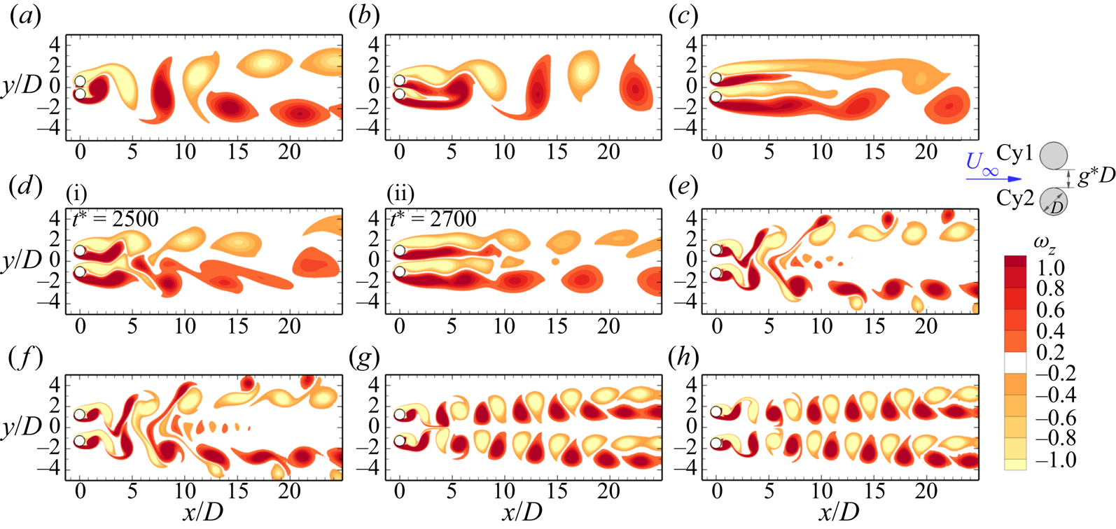
Figure 4. Instantaneous vorticity contours for 2-D periodic base flows; SS: symmetric single bluff-body vortex shedding, ASS: asymmetric bluff-body vortex shedding, FF: flip-flop vortex shedding, IP: in-phase vortex shedding, AP: anti-phase vortex shedding and  $\textrm {IP}_B$: in-phase biased vortex shedding. Results are shown for (a) SS at
  $(g^*, Re) = (0.1, 85)$; (b) ASS at
  $(g^*, Re) = (0.3, 100)$; (c)
  $\textrm {IP}_B$ at
  $(g^*, Re) = (0.8, 72)$; (d-i) FF at
  $(g^*, Re) = (1.0, 75)$; (d-ii) FF at
  $(g^*, Re) = (1.0, 75)$; (e) IP at
  $(g^*, Re) = (1.2, 225)$; ( f) IP at
  $(g^*, Re) = (1.5, 225)$; (g) AP at
  $(g^*, Re) = (1.5, 225)$; and (h) AP at
  $(g^*, Re) = (2.0, 300)$.
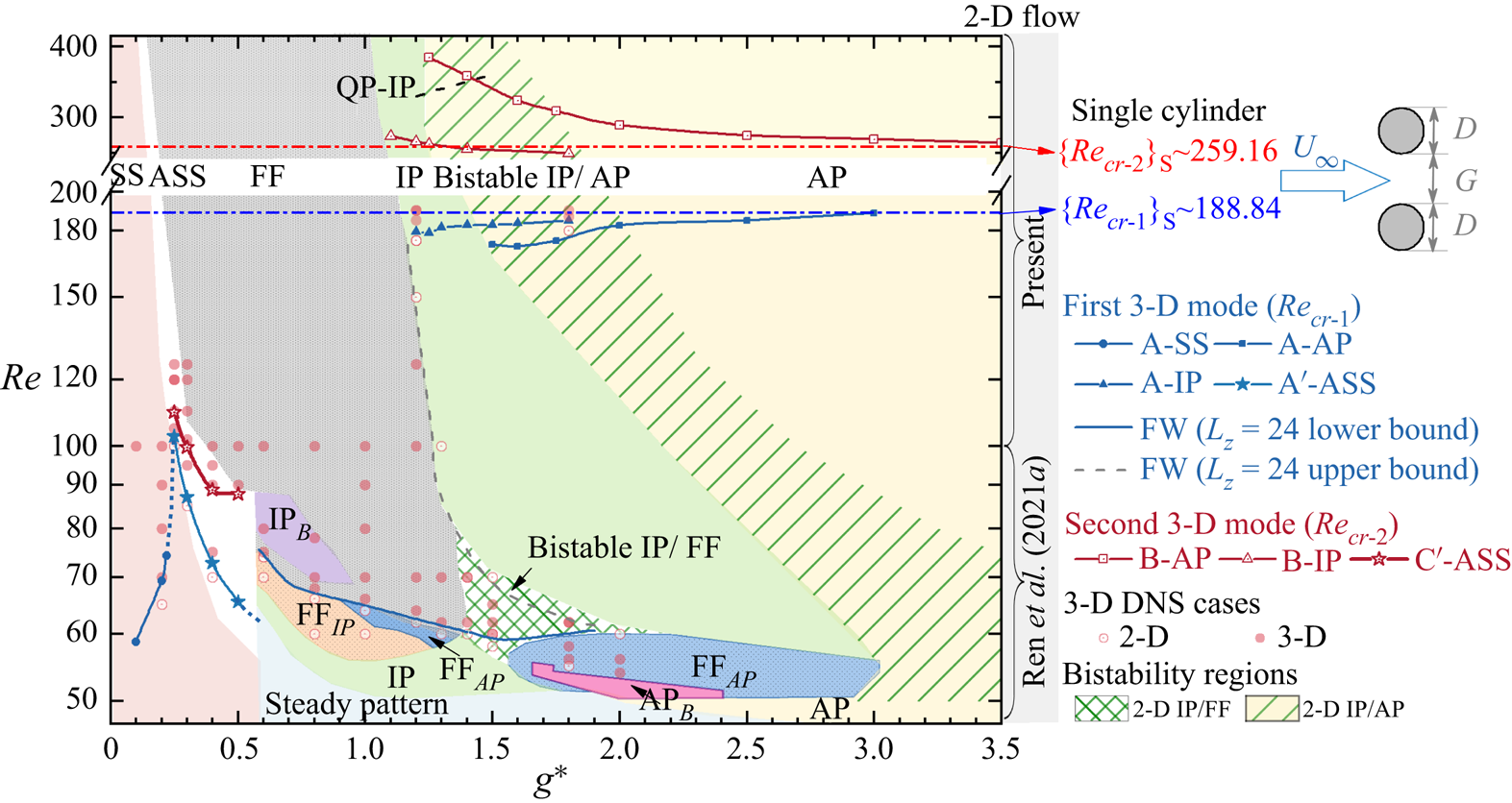
Figure 5. Distributions of critical  ${\textit {Re}}$ with respect to
  $g^*$ for the onset of 3-D instabilities in the wake of steady flow past two side-by-side circular cylinders. The dominant 2-D flow states are coloured by different backgrounds. Two bistable wakes, i.e. bistable IP/FF and bistable IP/AP, in 2-D simulations are marked as green meshes and inclined green lines, respectively. The dashed dot lines in blue and red represent the respective
  $\{{\textit {Re}}_{cr-1}\}_S$ and
  $\{{\textit {Re}}_{cr-2}\}_S$ obtained from figure 2. The solid and hollow circles indicate the flow with and without 3-D structures in 3-D DNS.
5. Three-dimensional wake transitions
In this section, wake transitions to 3-D flow are investigated. Floquet analysis is conducted for coupled-individual wake (IP and AP) and single bluff-body wake (SS, ASS and  $\textrm {IP}_B$) flows. The 3-D DNS is adopted to explore the physics behind the observed flow, and for FF flows where the Floquet analysis is deemed to be inappropriate.
By taking the advantage of the existing acronyms of 3-D instabilities for flow past an isolated cylinder, e.g. mode A, mode B and mode C, the present study defines different types of 3-D instability in terms of their RT symmetries along the wake centreline and base flow characteristics. For instance, the nomenclature of ‘mode A-IP’ represents the mode A-type instability that bifurcates from the 2-D IP base flow. Its critical  ${\textit {Re}}$ and
  $\lambda$ are denoted as
  ${\textit {Re}}_{cr-A}$ and
  $\lambda _{cr-A}$, respectively. Universally,
  ${\textit {Re}}_{cr-1}$/
 $\lambda _{cr-1}$ and
  ${\textit {Re}}_{cr-2}$/
 $\lambda _{cr-2}$ used in this paper indicate critical values associated with the onsets of first and second 3-D instability modes that appear in terms of
  ${\textit {Re}}$. To simplify the discussion, corresponding values of the single circular cylinder counterparts are denoted as
  $\{ {\cdot } \}_S$.
The critical  ${\textit {Re}}_{cr}$ for various 3-D instabilities as a function of
  $g^*$ are identified in figure 5, along with 2-D flow states shaded as background. The dominant spanwise wavelength for selected 3-D instabilities are compared in figure 6 with those from the single-cylinder counterpart. The boundary for each type of base flow is plotted as a blue line in figure 5. The blue dots at
  $g^* < 0.6$ are the estimated
  ${\textit {Re}}_{cr-1}-g^*$ boundaries connecting solid blue lines. Since not all base flow states own the second 3-D mode, the critical
  ${\textit {Re}}_{cr-2}-g^*$ curves are plotted as red lines in figure 5.

Figure 6. Dominant spanwise wavelength  $\lambda$ at the onset of 3-D instabilities with respect to
  $g^*$. The same line legends of flow states as detailed in figure 5 are used. Three horizontal lines indicate the critical spanwise wavelengths for flow past an isolated circular cylinder, including the first 3-D mode
  $(\{\lambda _{cr-1}\}_S)$, the second 3-D mode
  $(\{\lambda _{cr-2}\}_S)$ and
  $2 \{\lambda _{cr-1}\}_S$.
The wake interference significantly changes the occurrence of 3-D modes; and the first and second 3-D modes do not always manifest as the respective mode A type and mode B type. The following observations are noteworthy based on the results shown in figures 5 and 6.
(i) At small
$g^* \lessapprox 0.25$ with the SS regime as the base flow, only mode A is detected at much smaller ${\textit {Re}}_{cr-1}$ than its counterpart for a single cylinder $\{{\textit {Re}}_{cr-1}\}_S$. The ${\textit {Re}}_{cr-1}$ ranges between 30 %–50 % of $\{ {\textit {Re}}_{cr-1}\}_S$ due to the large length scale of the wake behind two cylinders at small gap ratios. The length scale of the SS wake is approximately $2D+g^*D$. The increase of ${\textit {Re}}_{cr-1}$ with increasing $g^*$ is associated with the weakening of cluster shear layers. The quantitative reasoning is provided in § 5.1.1. The value of $\lambda _{cr-1}$ is less sensitive to $g^*$ and amounts to more than twice of $\{\lambda _{cr-1}\}_S$. No mode B is predicted by the Floquet analysis.(ii) When the ASS flow develops, two new unstable modes are predicted by the Floquet analysis. They are termed as mode A
$'$ and mode C$'$ because their spatio-temporal symmetries are analogous respective to the modes A and C instabilities of a single cylinder (Williamson Reference Williamson1996b) but with different characteristics of 3-D modes, which will be introduced in §§ 5.1 and 5.2. The appearance of the subharmonic mode C$'$ as the second 3-D mode is thought to be associated with the breaking of spatio-temporal symmetry in the ASS base flow. The ${\textit {Re}}_{cr-1}$ and ${\textit {Re}}_{cr-2}$ values in this region show decreasing trends with increasing $g^*$ and are of a similar order of magnitudes to the ${\textit {Re}}_{cr-1}$ of SS. The $\lambda _{cr-1}$ and $\lambda _{cr-2}$ for mode A$'$ and mode C$'$ increase with ascending $g^*$ and amount to more than two times their single-cylinder counterparts.(iii) The 3-D instability for the FF wake at
$g^* = 0.6\unicode{x2013} 2.0$ is developed at ${\textit {Re}} \approx 75\unicode{x2013} 60$ and is substantially smaller than $\{ {\textit {Re}}_{cr-1}\}_S$ due to the strong irregular wake. This 3-D mode is termed the mode flip-flop wake (FW) as no ordered 3-D structure is identifiable.(iv) In the top-right corner of the transition map where the flows are in IP, bistable IP/AP and AP states, the Floquet analysis results are somewhat similar to those of an isolated cylinder with mode A as the most unstable mode and mode B as the second mode for each type of base flow. The
${\textit {Re}}_{cr-1}$ and ${\textit {Re}}_{cr-2}$ values for IP flows are greater and smaller than their AP flow counterparts, respectively. They both show respective increasing and decreasing trends with increasing $g^*$ in this region and converge towards their counterparts of an isolated cylinder. The $\lambda _{cr-1}$ and $\lambda _{cr-2}$ of IP flow are almost identical to the respective values of $\{\lambda _{cr-1}\}_S$ and $\{\lambda _{cr-2}\}_S$ and slightly larger than their AP flow counterparts.(v) The bistabilities (1) between 2-D and 3-D flows or (2) between different 3-D modes are detected in the regions where the bistable IP/FF and IP/AP are identified in 2-D DNS (Ren et al. Reference Ren, Cheng, Xiong, Tong and Chen2021a). This aspect will be elaborated further in § 5.4.


The above observations affirm that the 2-D base flow characteristics have significant impact on the wake transition and the 3-D modes. Detailed demonstrations and physical interpretations of the first and second 3-D modes are provided in §§ 5.1 and 5.2, respectively. The analyses and discussions are particularly centred around interpretations of the physical mechanisms responsible for the distinct  ${\textit {Re}}_{cr} - g^*$ correlations for different base flows observed in figure 5.
5.1. First 3-D instability
5.1.1. Single bluff-body wake
For  $g^*<0.25$, where the base flow is in SS, the results from Floquet analysis show that the onset of three-dimensionality develops at extremely low
  ${\textit {Re}}$, which ranges between 30 %–50 % of
  $\{{\textit {Re}}_{cr-1}\}_S \approx 188.84$ (figure 5). The small
  ${\textit {Re}}_{cr-1}$ can be attributed to the weaker gap flow at small
  $g^*$, causing the cylinder group to resemble a single bluff object with an effective length scale of approximately
  $2D+g^*{D}$ rather than
  $D$ of its single-cylinder counterpart. The single bluff object introduces a wider wake (Roshko Reference Roshko1954) and, hence, a smaller
  ${\textit {Re}}_{cr-1}$ related to the onset of 3-D transition. This also explains the large
  $\lambda _{cr-1}$ of SS base flow shown in figure 6.
The spatial distribution of the  $\hat {\omega }_x$ field (figure 7a) for the unstable mode (with real and positive
  $\mu$) is similar to the mode A of a single cylinder, where high concentrations of
  $\hat {\omega }_x$ are located close to the vortex cores. With increasing
  $g^*$, the gap flow and the outer shear layers are strengthened and weakened, respectively, resulting in a weaker single bluff-body wake generated by the two cylinders. The weakening process is first supported by the quantification of the strength of shed vortices with varying
  $g^*$ at
  ${\textit {Re}} = 80$. Figure 7(c) shows the instantaneous strengths of a pair of shed vortices, represented by the
  $|\omega _z|$ values at vortex cores (see
  $\varOmega _1$ and
  $\varOmega _2$ in figure 7a), at the phase where
  $C_{L-1}$ reaches local maxima. As
  $g^*$ increases, the strength of both negative (
 $\varOmega _1$) and positive (
 $\varOmega _2$) shed vortices decrease, indicating a weakening of the outer shear layers. This weakening process is further evident in the location of the wake recirculation bubble, obtained from the time-averaged flow fields over 20 vortex shedding periods. In the presence of gap flow the wake recirculation bubble detaches from the cylinder surfaces and forms two wake stagnation points, namely
  $x_{s1}$ and
  $x_{s2}$, as shown in figure 7(d) at
  $(g^*, Re) = (0.2, 80)$. The bubble moves downstream with increasing
  $g^*$ until it disappears when the spatio-temporal symmetry breaks (e.g. at
  $g^* = 0.3$ for
  ${\textit {Re}} = 80$). Due to the increased gap flow and the weakened outer shear layer with increasing the
  $g^*$, the two wake stagnation points are formed further downstream as displayed in figure 7(d). Therefore, we attribute the increase of
  ${\textit {Re}}_{cr-1}$ with
  $g^*$ for the SS base flow to the weakening process of the single bluff-body wake.
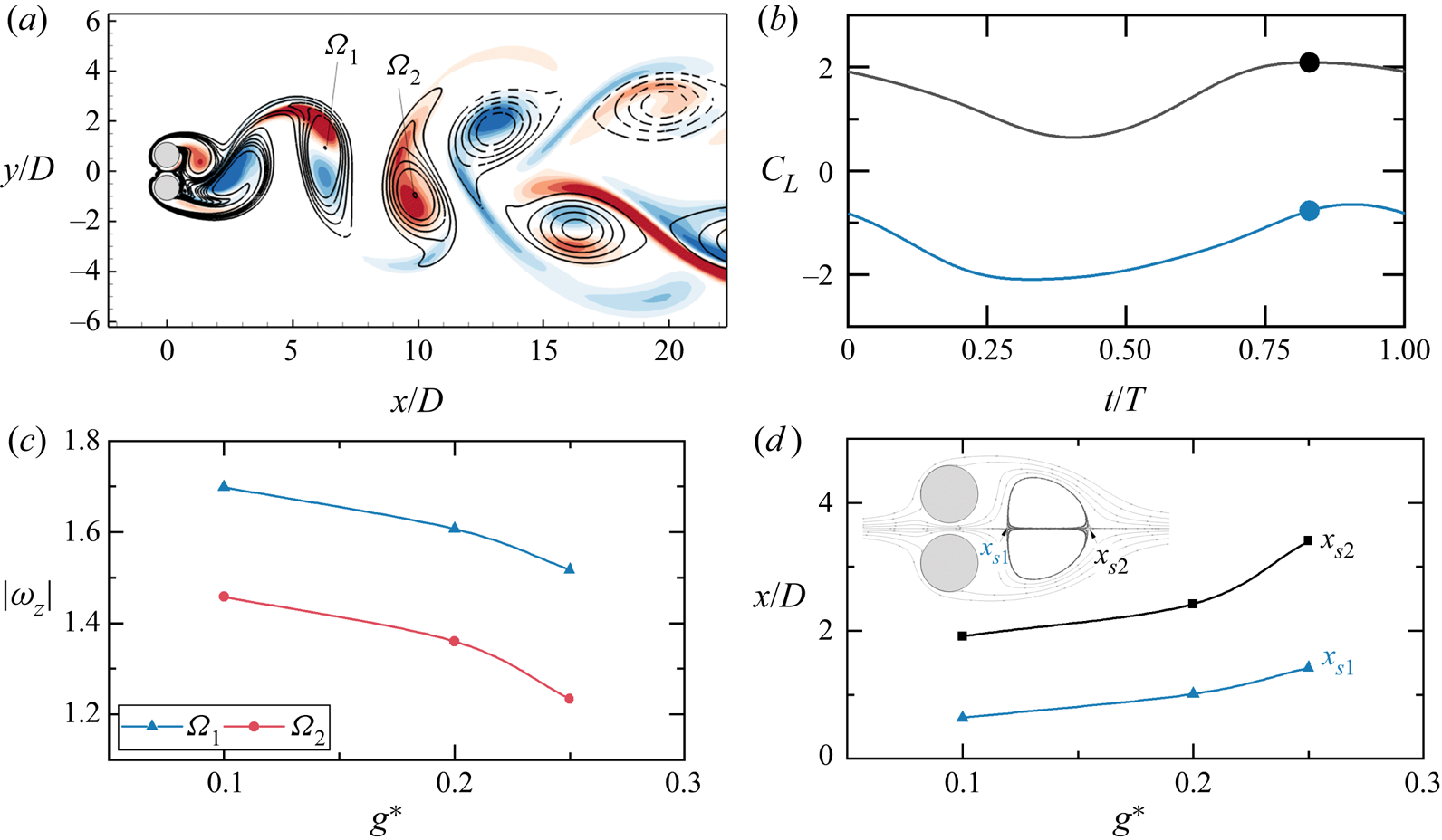
Figure 7. (a) The spatial distribution of  $\hat {\omega }_x$ contours for a mode A-SS at
  $(g^*, Re, \beta ) = (0.1, 80, 0.8)$ overlapped on base flow
  $\omega _z$ isolines at the instant where the lift coefficient of the top cylinder
  $C_{L-1}$ reaches a local maximum (the solid dots in (b)). (c) Variations of
  $|\omega _z| - g^*$ at
  $Re = 80$, where the blue and red curves are quantified as the cores of negative vortex
  $\varOmega _1$ and positive vortex
  $\varOmega _2$ at the instant shown as the solid dots in (b). (d) Variations of the wake stagnation points,
  $x_{s1}$ and
  $x_{s2}$, with respect to
  $g^*$ at
  $Re = 80$.
As  $g^*$ is increased to 0.25–0.6 in the ASS state, the wake transition to 3-D flow shows a distinct characteristic, as demonstrated in figure 8 at
  $g^* = 0.3$. The
  $|\mu | - \beta$ and
  $\lambda - {\textit {Re}}$ variations (figure 8a,b) suggest that the most unstable 3-D mode (real and positive
  $\mu$) occurs at
  ${\textit {Re}}_{cr-1} \approx 87.12$ with
  $\lambda _{cr-1} \approx 8.64$. The spatial and temporal distributions of the reconstructed flow field from Floquet analysis in figure 8(c,d) indicate that the
  $\hat {\omega }_x$ is slightly deflected upwards due to the downwards biased gap flow. High concentrations of
  $\hat {\omega }_x$ are located close to both vortex cores and braid shear layers. The
  $\hat {\omega }_x$ field in figure 8(c) differs from that of the typical mode A (figure 3b-i) in a sense that the
  $\hat {\omega }_x$ values in neighbouring braid shear layers are of the same signs and weakly holds an even RT symmetry along
  $y_c/D \approx 0.5$. The
  ${\textit {Re}}_{cr-1}$ decreases from around 102 to 60 as
  $g^*$ increases from 0.25 to 0.6 (figure 5), forming an opposite trend to that of the SS flow. The
  $\lambda _{cr-1}$ of ASS flow amounts to more than two times the
  $\{\lambda _{cr-1}\}_S \sim 4D$ due to the single bluff-body wake of ASS flow. The
  $\lambda _{cr-1}$ increases with
  $g^*$ and shows a rapid increase at
  $g^* = 0.4\unicode{x2013} 0.5$. The above variations of
  ${\textit {Re}}_{cr-1}$ and
  $\lambda _{cr-1}$ with
  $g^*$ suggest that the first 3-D mode of the ASS flow may be associated with the unique characteristics that exist in the base flow.
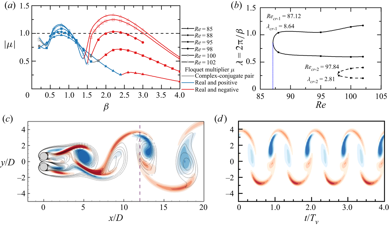
Figure 8. (a) Evolutions of the modulus of the Floquet multipliers  $|\mu |$ varying with the spanwise wavenumber
  $\beta$ for the ASS flow at
  $g^* = 0.3$, where
  $\mu$ values with complex conjugate, real and positive and real and negative are marked as grey, blue and red colours, respectively. (b) Corresponding neutral stability curves plotted in the
  ${\textit {Re}}$ and wavelength (
 $\lambda = 2{\rm \pi} /\beta$) space. (c) Spatial distribution of
  $\hat {\omega }_x$ field for a mode A
 $'$-ASS at
  $(g^*, Re, \beta )= (0.3, 100, 0.8)$. (d) The temporal evolution of
  $\hat {\omega }_x$ on the line of
  $x/D = 12$ over four vortex shedding periods (
 $T_v$).
The above distinct features for the ASS flow (e.g. decreasing trend of  ${\textit {Re}}_{cr-1}$ with
  $g^*$) are attributed to the disturbances of biased gap flow to the cluster shear layers around the cylinders. It is well known that the wake transition to 3-D flow is subcritical for an isolated cylinder (e.g. Williamson Reference Williamson1996b; Thompson et al. Reference Thompson, Hourigan, Ryan and Sheard2006) and the critical Reynolds number for the subcritical transition is dependent on the level of disturbances in the flow. Our DNS results (presented in § 5.3.3) confirm that the transition of 2-D ASS flow to 3-D flow is also subcritical. The disturbance level induced by the biased gap flow is likely dependent on the level of asymmetry of the base flow and the flow rate through the gap. To confirm our inference, we quantify the variations of flow asymmetry and flow rate with
  $g^*$ over
  $g^* = 0.2\unicode{x2013} 0.5$ in figure 9. The level of asymmetry of the base flow is quantified by
 \begin{equation} \varGamma=\sum_{i=1}^N \left|\iint_{\varOmega}\omega_z(t_i)\,\mathrm{d}\varOmega+ \iint_{\varOmega}\omega_z(t_{i+N/2})\,\mathrm{d}\varOmega\right|, \end{equation}
where  $N = 32$ is the equi-spaced snapshots over
  $1T_v$;
  $\varOmega$ is the integration region at
  $[-1\leq x/D \leq 10,\ -5 \leq y/D \leq 5]$. According to (4.1), the terms of
  $\iint _{\varOmega }\omega _z(t_i)\,\mathrm {d}\varOmega \ne -\iint _{\varOmega }\omega _z(t_{i+N/2})\,\mathrm {d}\varOmega$ when the spatio-temporal symmetry is broken. The magnitude of
  $\varGamma$ effectively measures the degree of the wake asymmetry during one vortex shedding cycle. The flow rate through the gap (
 $x/D = 0$) is defined as
 \begin{equation} \overline{U_{gap}}=\int_{{-}0.5g^*}^{0.5g^*} \overline{u(y)}\,\mathrm{d}y, \end{equation}
where the  $\overline {u(y)}$ is obtained from an averaged field over 100 non-dimensional time units. The results presented in figure 9(a) show that both
  $\varGamma$ and
  $\overline {U_{gap}}$ increase with increasing
  $g^*$, confirming our inference. The strengthened gap flow rate and the large asymmetry of the base flow provide a sustained disturbance to the flow, leading to the wake transition to 3-D flow at low
  ${\textit {Re}}$.
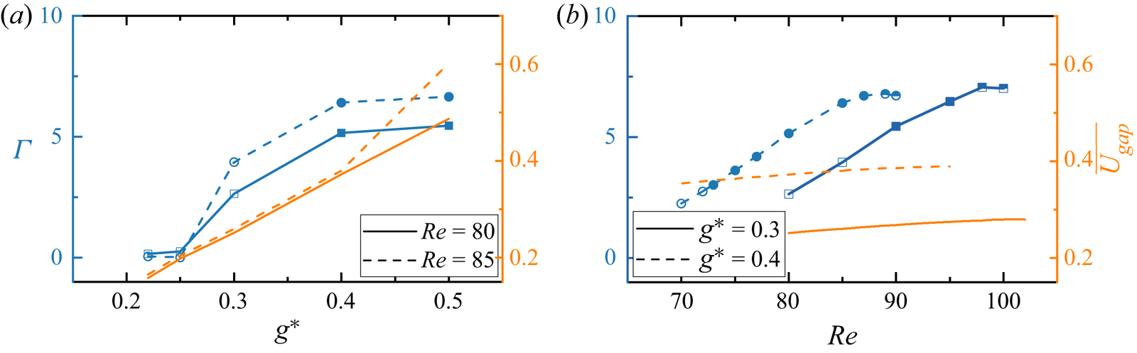
Figure 9. The variations of the extent of wake asymmetry  $\varGamma$ (left
  $Y$ axis) and gap flow rate
  $\overline {U_{gap}}$ (right
  $Y$ axis) with respect to (a)
  $g^*$ and (b)
  ${\textit {Re}}$ values. The solid and half-filled symbols indicate the occurrence of first and secondary 3-D instabilities, respectively.
The first 3-D mode for the  $\textrm {IP}_B$ base flow at
  $g^* = 0.6\unicode{x2013} 0.9$ forms the similar mode A
 $'$ structure, where the value of Floquet multiplier
  $\mu$ is real and positive. The large inclination of the upward biased gap flow initiates the mode A
 $'$ structure in the braid shear layers of the wake behind the bottom cylinder, as presented in the Floquet mode and linear reconstructed 3-D field in figures 10(a) and 10(b), respectively. In figures 5 and 6 we did not give the marginal curves of this mode. This is because, all the
  $\textrm {IP}_B$ base flows in the purple shaded region in figure 5 are unstable to the mode A
 $'$ instability, as confirmed by both Floquet analysis and 3-D DNS using
  $L_z = 28$. As the
  $\textrm {IP}_B$ flow below the purple shaded region in figure 5 cannot be simply generated by decreasing
  ${\textit {Re}}$ from a fully developed
  $\textrm {IP}_B$ flow, the exact
  ${\textit {Re}}_{cr-1} - g^*$ and
  $\lambda _{cr-1} - g^*$ curves for the
  $\textrm {IP}_B$ base flow are not provided. We anticipate that the
  ${\textit {Re}}_{cr-1}$ of mode A
 $'$ in
  $\textrm {IP}_B$ is likely lower than its dominant
  ${\textit {Re}}$ range in 2-D simulation and presumably follows the
  ${\textit {Re}}_{cr-1} - g^*$ trend of mode A
 $'$ in the ASS.

Figure 10. Same as figure 3 but for the mode A $'$-
$'$- $\textrm {IP}_B$ instability at
  $(g^*, Re, \beta )= (0.8, 72, 0.6)$. (a) Spatial distribution. (b) Reconstructed 3-D field.
5.1.2. Flip-flop wake
For flows in the FF regime, we could not perform Floquet analysis as the wake is aperiodic over each vortex shedding cycle. Therefore, we employed a series of 3-D DNS at  $g^* = 0.6\unicode{x2013} 2.0$ and
  ${\textit {Re}} = 55\unicode{x2013} 100$ to investigate its 3-D transition features. The 3-D DNS is conducted by using its fully developed 2-D counterpart as an IC; and the dimensionless length of the cylinder is selected as
  $L_z = 24$. The flow without and with 3-D instabilities are presented as hollow and filled circles in figure 5 in the region filled with FF flow. The development of 3-D flow is measured during the simulation through the evolutions of
  $\varepsilon _{xy}/\varepsilon _{t}$ in the near wake region of
  $[0 \leq x/D \leq 10,\ -5 \leq y/D \leq 5]$. In the present study the 3-D instability of the FF flow (mode FW) is identifiable when the
  $\varepsilon _{xy}/\varepsilon _{t} > 10^{-3}$; and we use this criteria to assess whether mode FW is developed.
The wake transition to 3-D flow for FF flow is rather interesting in figure 5. The  ${\textit {Re}}_{cr-1}$ experiences a step jump from
  ${\sim }65$ to
  ${\sim }75$ when the base flow changes from ASS to FF at
  $g^* \sim 0.6$. Further increasing
  $g^*$ over the FF range, the
  ${\textit {Re}}_{cr-1}$ for mode FW decreases till about
  $g^* = 1.5$, followed by a slight increase for
  $g^* \sim 1.5\unicode{x2013} 1.8$. The discontinuity at
  $g^* \sim 0.6$ suggests that the onset of 3-D instability for the FF flow may have been triggered by different flow characteristics compared with that of the ASS flow. We attribute it to the distinct irregular wake evolutions that exist in FF flow, which lead to the development of mode FW at such low
  ${\textit {Re}}_{cr-1}$. The decreasing trend of
  ${\textit {Re}}_{cr-1}$ with increasing
  $g^*$ for
  $g^* \leq 1.5$ is possibly related to the increasing level of wake irregularity. These conjectures are supported by the characteristics of the lift coefficients on the top and bottom cylinders, i.e.
  $C_{L,1}$ and
  $C_{L,2}$, respectively, and will be elaborated in the following paragraphs.
As an example, figure 11 shows the development of mode FW from a 2-D FF flow at  $g^* = 1.0$ and
  ${\textit {Re}} = 64\unicode{x2013} 100$. The force time histories in the blue shaded area (figure 11a–d) are those obtained from 2-D DNS; and the instantaneous flow field at the end of 2-D simulation (termed as
  $t_0$) is used for the subsequent 3-D DNS. Comparing the
  $C_{L,1}$ and
  $C_{L,2}$ time histories in 2-D and 3-D simulations, the lift coefficient evolutions in FF flows become much more complex as
  ${\textit {Re}}$ is increased. The development of mode FW does not change the synchronisation state of two wakes in the 2-D FF flow. In addition, the results in figure 11 demonstrate a strong correlation between the complexity of lift coefficients in the 2-D DNS (blue shaded area in figures 11a–d) and the development of the 3-D structure (flow fields in figures 11i–l). Specifically, the time history of
  $C_{L,1}$ and
  $C_{L,2}$ forms a transition from quasi-periodic evolutions to irregular evolutions at
  ${\textit {Re}}_{cr-1} \approx 66$, coinciding with the wake transition from 2-D FF flow to mode FW. To quantify this correlation, we calculate the fluctuation of the total lift coefficient peaks,
  $\varPsi$, which is defined as
 \begin{equation} \varPsi= RMS(C_{L,T}^{pks}-\overline{C_{L,T}^{pks}}), \end{equation}
where  $C_{L,T}^{pks}$ represents the local maxima of
  $C_{L,T} = C_{L,1}+C_{L,2}$;
  $\overline {C_{L,T}^{pks}}$ is the mean value of
  $C_{L,T}^{pks}$. The
  $\varPsi$ value is calculated through 2-D results because we believe that the irregularity triggering the 3-D transition largely originates from the 2-D flow.

Figure 11. Time histories of the lift coefficients (a–d) and  $\varepsilon _{xy}/\varepsilon _{t}$ (e–h) for FF flows at
  $g^*=1.0$ and
  ${\textit {Re}} = 64 -100$, where
  $t_0$ indicates the time instant where 3-D DNS starts. Instantaneous 3-D flows in the global view (i–l) and
  $x$–
$x$– $z$ plane view (m–p) of each case, where the isosurfaces are
  $\omega _x = \pm 0.4$ (blue and red) and
  $\omega _z = \pm 0.5$ (grey).
The evolutions of  $\varPsi$ with
  $g^*$ and
  ${\textit {Re}}$ are shown in figure 12(a) and 12(b), respectively, where flows that transition to mode FW are marked as solid symbols. Figure 12(a) suggests that at
  ${\textit {Re}} = 62$ the
  $\varPsi$ of FF flow increases with enlarging
  $g^*$ for
  $g^*\leq 1.7$, which agrees with our anticipation. Mode FW is observed when the
  $\varPsi$ manifests a large magnitude at
  $g^* = 1.3\unicode{x2013} 1.8$. The values of
  $\varPsi \approx 0$ at
  $g^* = 0.7$ and 2.0 are due to the flow transits to an IP state with periodic wakes behind two cylinders. The evolutions of
  $\varPsi$ with
  ${\textit {Re}}$ at different
  $g^*$ values (figure 12b) are not monotonic due to the complex flow state transitions. The initiations of mode FW with respect to
  ${\textit {Re}}$ are highly associated with the large magnitudes of
  $\varPsi$.
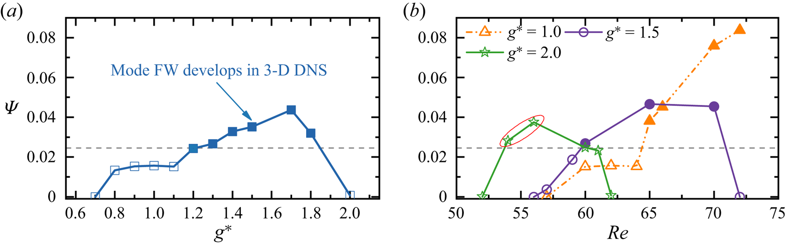
Figure 12. Evolutions of wake irregularity parameter,  $\varPsi$, with (a)
  $g^*$ at
  ${\textit {Re}} = 62$ and (b)
  ${\textit {Re}}$ at
  $g^* = 1.0, 1.5, 2.0$. The
  $\varPsi$ values are calculated based on 2-D results. The symbols filled by solid colours are cases where we observed mode FW in the 3-D DNS. Cases circled in red at
  $g^* = 2.0$ only transit to mode FW by using
  $L_z = 48$.
The relationship between  $\varPsi$ and the 3-D instability, except for
  $g^* = 2.0$, consistently shows that the 3-D instability occurs when
  $\varPsi > \sim 0.0245$ (the dashed grey line in figure 12). However, an exception is found at
  $g^* = 2.0$ where no identifiable 3-D instability is observed with
  $\varPsi = 0.376$ at
  ${\textit {Re}} = 56$. We suspect the discrepancy is caused by the use of
  $L_z = 24$ at large
  $g^*$, which may not be large enough for the mode FW to develop as the wavelength of the 3-D structure is expected to be large at low
  ${\textit {Re}}$ values. To confirm this inference, we conducted additional 3-D simulations for
  $g^* = 2.0$ using
  $L_z = 48$. As expected, the flows at
  ${\textit {Re}} = 54$ and 56, where
  $\varPsi > 0.0245$ in figure 12(b), transit into mode FW with weak 3-D structures (
 $\varepsilon _{xy}/\varepsilon _{t} \approx 10^{-3}$). No further investigations were conducted to seek the exact
  ${\textit {Re}}_{cr-1} - g^*$ boundaries. We anticipate the lower bound
  ${\textit {Re}}_{cr}$ at large
  $g^*$ may be slightly lower than that given in figure 5 and conversely, the upper bound
  ${\textit {Re}}_{cr-1}$ may be slightly higher.
We also note that the quantity  $\varPsi$ is an indicative correlation between 2-D wake irregularity and the development of mode FW. This argument is because, firstly, the
  $\varPsi$ in (5.3) is proposed under the assumption that the onset of mode FW is triggered by flow instabilities originating from the 2-D base flow. As the lift coefficients on cylinders are global parameters, the
  $\varPsi$ may not be the only parameter that determines the 3-D instability. In addition, the critical value of
  $\varPsi \sim 0.0245$ is ad hoc selected through figure 12 and may not be valid in other 3-D transition problems.
Another phenomenon for the 3-D transition of FF flow in figure 5 is that, over the range of  $g^* = 1.2\unicode{x2013} 1.8$, the flow transition sequence of ‘2-D FF
  $\to$ mode FW
  $\to$ 2-D IP
  $\to$ mode A-IP’ with increasing
  ${\textit {Re}}$. This phenomenon differs from the single-cylinder counterpart where the wake remains in 3-D flow and becomes increasingly irregular with increasing
  ${\textit {Re}}$. This transition sequence is further affirmed to be physical by conducting 3-D DNS for
  $g^* = 1.2$ and
  ${\textit {Re}} = 58\unicode{x2013} 190$, where 2-D and 3-D flows are plotted as discrete hollow and solid symbols in figure 5. The spanwise lengths
  $L_z = 24$ and
  $4{\rm \pi}$ are used for cases at
  ${\textit {Re}} < 100$ and
  ${\textit {Re}} > 100$, respectively. The distinct transition that exists here is because flow characteristics in FF and IP flows have different wake interference on the development of 3-D instability. Precisely, when the wake irregularity is relatively weak, mode FW transits back to a 2-D flow when
  ${\textit {Re}}$ approaches the upper bound of the FF flow region (dashed grey line in figure 5). Further increasing
  ${\textit {Re}}$ in the IP flow till
  ${\textit {Re}} \sim 180$, the elliptical instability of primary vortex cores in the IP wake develops, constituting the development of mode A-IP.
Detailed characteristics of mode FW are discussed using cases shown in figure 11. Since the transition of 2-D FF to mode FW cannot be predicted through Floquet analysis, we apply the Hilbert transform (Kress, Maz'ya & Kozlov Reference Kress, Maz'ya and Kozlov1989) to quantify the spatial distribution of spanwise length scales in mode FW and their evolutions with  ${\textit {Re}}$. For each
  $(x, y)$ location, the spanwise wavelength is obtained by analysing the Hilbert transform of
  $\omega _y$ along
  $z$. The localised spanwise length scale
  $\lambda _z$ is estimated as
 \begin{equation} \frac{2{\rm \pi}}{\lambda_z} = \frac{\mathrm{d} \phi_{\omega_y}(z,t)}{\mathrm{d}z}, \end{equation}
where  $\phi _{\omega _y}(z,t) \equiv \textrm {arg}[\omega _y(z,t)]$ is the spanwise phase of
  $\omega _y(z,t)$ calculated from the Hilbert transform as
 \begin{equation} \omega_y(z,t) \equiv A_{\omega_y}(z,t) \exp({{\rm i}\phi_{\omega_y}(z,t)}), \end{equation}
where  $A_{\omega _y}(z, t) \equiv |\omega _y(z, t)|$ is the local amplitude. Following the work by Sarwar & Mellibovsky (Reference Sarwar and Mellibovsky2020), (5.4) and (5.5) are calculated by adopting the approximation of
  $\omega _y \approx \partial u/\partial z$. The probability density function (PDF) of
  $\lambda _z$ along the
  $z$ direction, namely
  $\lambda _z^P$, is then used to characterise the distributions of
  $\lambda _z$. This method is superior for characterising the length scale of the flow with localised flow features and has also been used in the studies of wake flows behind a bluff body (Sarwar & Mellibovsky Reference Sarwar and Mellibovsky2020; Ong & Yin Reference Ong and Yin2022).
As an example, figure 13(a) displays the  $\lambda _z^P - t^*$ contour in a near wake region of
  $(x, y) = (8, 0)$ at
  $(g^*, {\textit {Re}}) = (1.0, 80)$, where the dark contours indicate the most representative length scales. The energetic spanwise structure in figure 13(a) has a length scale of
  $\lambda \sim 5D$. Figure 13(b) shows the averaged value of the PDF over 100 non-dimensional time units; and the maximum
  $\lambda _z^P$,
  $\lambda _{z,m}$, is used as the most representative spanwise length scale at (
 $x, y$). The
  $\lambda _{z,m}$ of mode FW along the wake centreline of
  $x/D = 2\unicode{x2013} 10$ for cases in figure 11 are shown in figure 13(c). At a fixed
  ${\textit {Re}}$, e.g.
  ${\textit {Re}} = 66$, the
  $\lambda _{z,m}$ decreases monotonically with
  $x/D$ for
  $x/D> 2$ due to the break up of large-scale vortices into small-scale vortices. With ascending
  ${\textit {Re}}$ from 66 to 100,
  $\lambda _{z,m}$ is reduced significantly and nearly unchanged over
  $x/D = 5\unicode{x2013} 10$. We acknowledge that the approximation of
  $\omega _y \approx \partial u/\partial z$ is used in estimating the characteristic length scale of mode FW. As demonstrated in Appendix B, this approximation may lead to a smaller
  $\lambda _{z,m}$. We recognise that the magnitude of
  $\lambda _{z,m}$ in figure 13(c) may vary slightly if different vorticity or velocity components are used. However, the trends of
  $\lambda _{z,m}$ with respect to
  $x/D$ and
  ${\textit {Re}}$ for mode FW would remain similar.
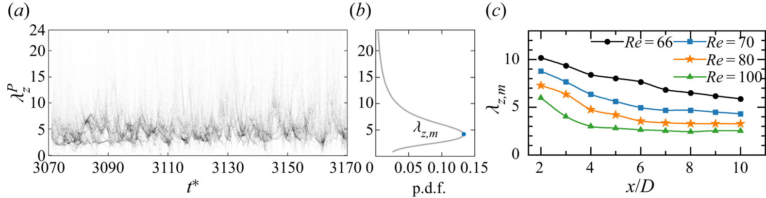
Figure 13. (a) Time evolution of PDF of the instantaneous spanwise wavelength  $\lambda _z^P$ distribution at a point in the near wake region of
  $(x, y) = (8, 0)$ for mode FW at
  $(g^*, {\textit {Re}})= (1.0, 80)$. (b) Time-averaged PDF distribution over 100
 $t^*$. The maximum
  $\lambda _z^P$ (
 $\lambda _{z,m}$, the blue dot) is used as the representative spanwise length scale at this point. (c) The most probable wavelength,
  $\lambda _{z,m}$, along the wake centreline (
 $y/D = 0$) for mode FW at
  $(g^*, {\textit {Re}}) = (1.0, 66\unicode{x2013} 100)$.
The evolutions of instantaneous 3-D flow fields show that the 3-D structures of mode FW flap over intermittently between two wakes and persist different strengths over time. The evolution of 2-D flow fields indicates that the gap flow of FF undergoes oscillations over each vortex shedding cycle. At small  $g^*$, the gap flow inclination leads to the weakening of vortex shedding around the cylinder in the direction of its inclination, while the vortex shedding on the other cylinder is strengthened. This strengthening/weakening process is also present in mode FW and is responsible for the flapping-over character of 3-D structures behind both wakes. This conjecture is validated through a case near the onset transition boundary, e.g.
  $(g^*, {\textit {Re}}) = (1.0, 66)$. Figure 14(a) displays the transverse velocity
  $v$ (grey line) for a point at the end of gap
  $(x/D, y/D, z/D) = (0.5, 0, 12)$. The averaged value of
  $v(t)$ between successive peaks and troughs (the dashed orange line), which represents the mean gap flow inclination direction in each half of the vortex shedding cycle, undergoes a slow and random flapping motion over several vortex shedding periods. Good correlations between the gap flow inclination (indicated by averaged
  $v(t)$) and strengthening/weakening of 3-D instabilities are observed. For instance, as the mean gap flow flaps to
  $y/D > 0$ from its equilibrium position (figure 14b–d), the vortex shedding from the top cylinder is weakened, characterised by an increase of wake formation length and the weakening of vortices (N1–N3) shed from the top shear layer. The 3-D structure in the wake of the top cylinder is weakened as well, as indicated by the weakening of
  $\omega _x$ fields in the shear layers of the top cylinder. During the same period of
  $t^* \approx 3010\unicode{x2013} 3030$, the strengthening of vortex shedding and 3-D instability from the bottom cylinder are observed. The observed behaviours over the next period of
  $t^* \approx 3030\unicode{x2013} 3050$, when the mean gap flow flaps to
  $y/D < 0$ (figure 14e–g) from its equilibrium position, are opposite to those in figure 14(c,d).
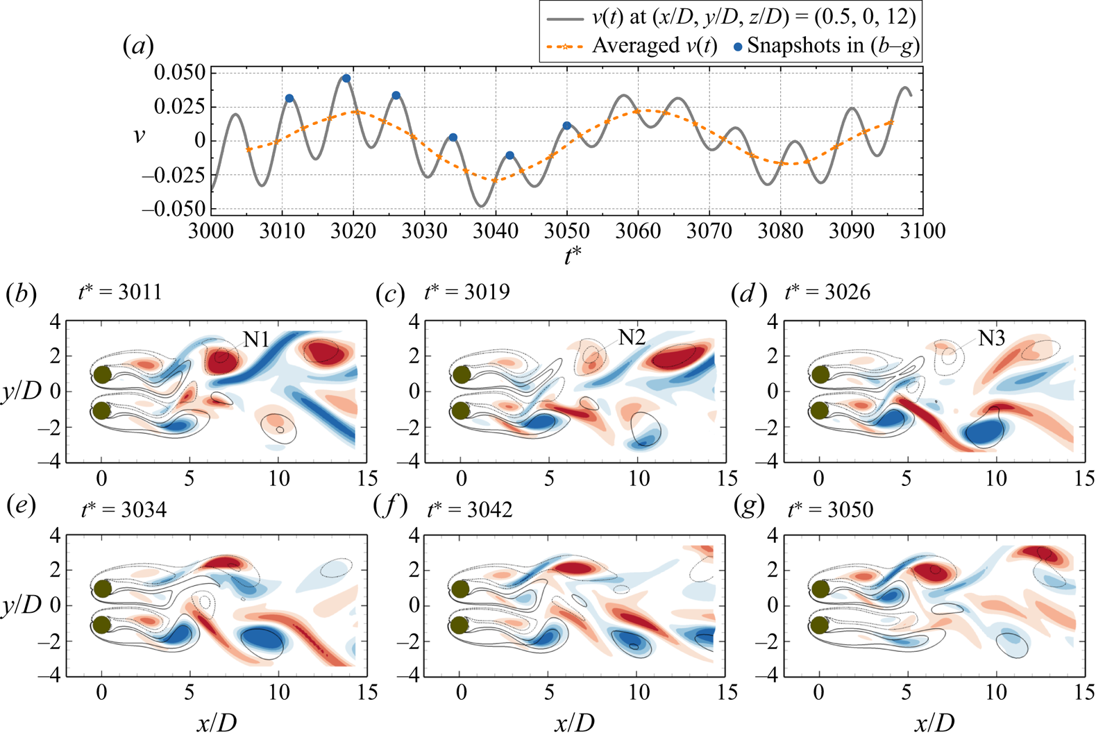
Figure 14. Evolutions of (a) the transverse velocity  $v$ at the end of the gap of
  $(x/D, y/D, z/D) = (0.5, 0, 12)$ and (b–g) the flow fields
  $x$–
$x$– $y$ plane at
  $z/D = 12$, sampled at the phases corresponding to the crests of
  $v(t)$ (blue circles) in (a) for the FF flow at
  $(g^*, {\textit {Re}})= (1.0, 66)$. The positive and negative
  $\omega _x$ fields are represented by the red and blue contours, respectively. The overlapped solid and dashed black lines are the corresponding positive and negative
  $\omega _z$ contours.
The above discussion suggests that, in two interacting wakes, the wake irregularity plays a pivotal role in triggering the 3-D instability. The onset transition from FF flow to mode FW develops at  ${\textit {Re}}$ significantly lower than the single-cylinder counterpart
  $\{ Re_{cr-1} \}_S = 188.84$.
5.1.3. Coupled wakes
For the flows in IP, bistable IP/AP and AP states, the onset 3-D wake transitions are similar to the results of the flow around a single cylinder, where an unstable region with real and positive  $\mu$ is identified at
  $\beta \approx 1.6\unicode{x2013} 1.8$. Mode A bifurcates slightly earlier in terms of
  ${\textit {Re}}$ than the single-cylinder case. With increasing
  ${\textit {Re}}$, the flow transition sequence is in ‘2-D
  $\to$ mode A
  $\to$ mode B’ for each type of base flow. The most unstable Floquet modes are similar to mode A of a single-cylinder case, except that the
  $\hat {\omega }_x$ fields behind both cylinders are modulated by the base flow symmetry conditions (4.1), (4.2). Similar 3-D transitions have been observed for steady flow past two side-by-side square cylinders (Choi & Yang Reference Choi and Yang2013). The effects of IP and AP wake couplings on the 3-D transitions of two circular cylinders in a side-by-side arrangement are discussed below.
The AP wake coupling destabilises the 3-D wake transition to a slightly lower  ${\textit {Re}}$ level, as illustrated in figure 15. This phenomenon is attributed to the confinement effect of the AP flow, which strengthens the vortex shedding process of each wake. This conjecture is firstly supported by the vortex shedding frequency (
 $f_{St}$) shown in Ren et al. (Reference Ren, Cheng, Tong, Xiong and Tang2023), where
  $f_{St}$ is slightly larger than the single-cylinder value at the corresponding
  ${\textit {Re}}$. As the interaction of vortex cores in each wake of AP is stronger than the unconfined wake, it constitutes the earlier initiation of mode A. As
  $g^*$ ascends, the AP confinement effect reduces gradually and the
  ${\textit {Re}}_{cr-1}$ asymptotes to the values of a single cylinder. The differences of
  ${\textit {Re}}_{cr-1}$ in AP from
  $\{{\textit {Re}}_{cr-1} \}_S$ is around 2.3 % at
  $g^* = 3.0$, suggesting that there are negligible differences (within 3 % tolerance) in the 3-D transitions between an isolated cylinder and the AP wake for
  $g^* > \sim 3$. In addition, a similar variation of
  ${\textit {Re}}_{cr-1}$ over
  $g^*$ has been found in other 3-D transition studies on a confined cylinder wake, i.e. the study of steady flow past an isolated cylinder near a moving wall (Jiang et al. Reference Jiang, Cheng, Draper and An2017a,Reference Jiang, Cheng, Draper and Anb), in which the variation was attributed to the reduced confinement of the moving wall. Given the cylinder wakes in both scenarios are confined by the presence of a moving wall (Rao et al. Reference Rao, Thompson, Leweke and Hourigan2015; Jiang et al. Reference Jiang, Cheng, Draper and An2017a) or the other wake (the present scenario), we believe the increase trend of
  ${\textit {Re}}_{cr-1}$ over
  $g^*$ in AP flow is indeed affected by the weakening of wake confinement. To further compare the wall confinement effect on two scenarios, the onset
  ${\textit {Re}}_{cr-1} - g^*$ curves for the AP base flow and moving wall case (Jiang et al. Reference Jiang, Cheng, Draper and An2017a) are shown in figure 15. We observe that, at
  $g^* > 1.5$, both the magnitude of
  ${\textit {Re}}_{cr-1}$ and its variation trend with respect to
  $g^*$ for AP base flow and the moving wall case at an equivalent gap distance are close, with the largest difference of 1.27 % occurring at
  $g^*=2.0$. This good agreement also suggests the confinement in the AP wake is comparable to the cylinder next to a moving wall.

Figure 15. The influence of wake confinement on the critical  ${\textit {Re}}$ of 3-D wake transitions of a steady flow past two side-by-side cylinders in the AP flow (present) and an isolated cylinder near a moving wall (Rao et al. Reference Rao, Thompson, Leweke and Hourigan2015; Jiang et al. Reference Jiang, Cheng, Draper and An2017a,Reference Jiang, Cheng, Draper and Anb). The gap-to-diameter ratio
  $G^*$ in Jiang et al. (Reference Jiang, Cheng, Draper and An2017a,Reference Jiang, Cheng, Draper and Anb) and Rao et al. (Reference Rao, Thompson, Leweke and Hourigan2015) is translated to
  $g^* = 2G^*$.
For the first 3-D instability of the IP base flow, i.e. mode A, the  ${\textit {Re}}_{cr-1}-g^*$ curve is very close to that of the single cylinder. This result is expected because the two IP wakes oscillate together with almost no confinement effect between wakes, compared with the strong confinement effect in the AP state. Even though the IP state has stronger wake coupling than the AP state, judging based on the sequence of their emergence in terms of enlarging
  $g^*$, the coupling is mainly related to the vortex merging in the downstream, which has a minor effect on the vortex shedding processes in the near wake. Consequently, the development of the first 3-D instability (mode A-IP) is less affected.
The above observations also suggest the wake confinement in AP is more favourable of interfering the 3-D instability than the vortex merging in the IP state.
5.2. Second 3-D instabilities
The Floquet analyses also identify the other 3-D instability modes that develop above  ${\textit {Re}}_{cr-1}$. The value of
  ${\textit {Re}}$ for the onset of the second 3-D mode is denoted as the
  ${\textit {Re}}_{cr-2}$. The present Floquet analysis identifies the second 3-D mode under the ASS, IP and AP base flow conditions.
5.2.1. Single bluff-body wake
The second 3-D instability for the ASS flow develops at large  $\beta$ number, as shown in figure 8(a), whose Floquet multiplier
  $\mu$ in the peak region is real and negative. Spatial and temporal distributions of a typical secondary unstable mode in ASS at
  $(g^*, Re, \beta ) = (0.3, 100, 2.4)$ are shown in figure 16. A period-doubling feature of the perturbed Floquet mode is identified. The symmetry condition of perturbed
  $\hat {\omega }_x$ field can be expressed as
 \begin{equation} \mbox{Mode C}': \begin{cases} \hat{\omega}_x(x,y,t)={-}\hat{\omega}_x(x,y,t+T_v), \\ \hat{\omega}_x(x,y,t)=\hat{\omega}_x(x,y,t+2T_v). \end{cases} \end{equation}
Equation (5.6) suggests that this mode takes two periods of vortex shedding in the  $x$–
$x$– $y$ plane to complete one cycle of spanwise structure evolution in the wake. The 3-D instability that holds the same RT symmetry condition as (5.6) is commonly denoted as the mode C-type instability in literature (Zhang et al. Reference Zhang, Fey, Noack, König and Eckelmann1995; Carmo et al. Reference Carmo, Sherwin, Bearman and Willden2008; Sheard et al. Reference Sheard, Fitzgerald and Ryan2009). For this reason, we refer to this mode to as ‘mode C
 $'$’. Similar to mode B of an isolated cylinder, the
  $\hat {\omega }_x$ field of mode C
 $'$ is concentrated in the braids.

Figure 16. (a) Spatial and (b) temporal distributions for mode C $'$-ASS at
  $(g^*, Re, \beta ) = (0.3, 100, 2.4)$. (c) The
  $|\mu | - \beta$ variations for two side-by-side cylinders with a diameter ratio of 1/0.8 at
  $g^* = 0.3$. (d) Spatial distribution for the unstable mode (mode C
 $'$ type) at
  $(Re, \beta ) = (100, 2.4)$.
Bearing in mind that mode C is absent in flow around an isolated cylinder, we anticipate that the formation of an asymmetric wake induced by the biased gap flow is responsible for the occurrence of mode C $'$ in the ASS flow. One evidence for this conjecture is from figure 9(b), where large magnitudes of
  $\varGamma$ and
  $\overline {U_{gap}}$ are observed when the ASS base flow forms mode C
 $'$ (half-filled symbols). To further confirm that the present mode C
 $'$ has similar features to the typical mode C that is triggered by asymmetric geometry configurations, we artificially reduce the diameter of the bottom cylinder to
  $0.8D$, while keeping the gap distance as
  $0.3D$. Floquet analyses are conducted over the range of
  ${\textit {Re}}$ (
 $= 90\unicode{x2013} 105$) to assess if mode C
 $'$ would develop. The
  $|\mu | - \beta$ variations in figure 16(c) show that an unstable region is identified in the vicinity of
  $\beta \sim 2.4$. Corresponding spatial distribution of the Floquet mode at
  $({\textit {Re}}, \beta ) = (100, 2.4)$ is shown in figure 16(d). The similarities in the
  $\hat {\omega }_x$ field and the
  $\beta$ ranges between the unstable modes in figure 16(c,d) and mode C
 $'$-ASS in figures 8(a) and 16(a) are clearly observed. In light of the above, it is therefore reasonable to conclude that mode C
 $'$ would develop when the wake asymmetry, induced by either the flow or geometry configuration, exceeds a critical value.
5.2.2. Coupled wakes
For the IP and AP coupled wakes, the second 3-D instability with real and positive  $\mu$ is of mode B type behind each cylinder, where
  $\hat {\omega }_x$ field intensifies in the near wake region and rapidly diminishes downstream of the cylinders. Due to the IP and AP coupling between two wakes, the mode B structure behind each cylinder is modified by the base flow symmetry conditions so that the mode B of AP and IP flows show a reflection symmetry and a spatio-temporal symmetry along
  $y_c/D = 0$, respectively.
The onset of mode B for the AP base flow is delayed to much higher  ${\textit {Re}}$, e.g.
  ${\textit {Re}}_{cr-2} \approx 359$ for
  $g^* = 1.4$ in figure 15. With an increase of
  $g^*$, the
  ${\textit {Re}}_{cr-2}$ of AP decreases monotonically to the value that is comparable to
  ${\textit {Re}}_{cr-2}$ of a single cylinder. The mechanism responsible for the large
  ${\textit {Re}}_{cr-2}$ is investigated by comparing the base flow characteristics of a single wake and the AP coupled wakes at
  ${\textit {Re}} = 300$ (see figures 3 and 4h). It is evident that the AP flow is featured by a stronger vortex shedding process than the single cylinder judging based on the strong vortices shed from the shear layers in figure 4(h). The braid shear layer of the AP flow, which connects adjacent vortex cores, is somewhat weakened. Since mode B is originated from the hyperbolic instability of the braid shear layer region (Williamson Reference Williamson1996a), the initiation of mode B is therefore delayed to much higher
  ${\textit {Re}}$ in AP. We attribute the weakening of the braid shear layer in AP to the wake confinement effect. This conjecture can be supported by the previous study of steady flow past an isolated cylinder near a moving wall (Rao et al. Reference Rao, Thompson, Leweke and Hourigan2015), where
  ${\textit {Re}}_{cr-2}$ gradually approaches
  $\{{\textit {Re}}_{cr-2}\}_S$ when the wall confinement is reducing (solid purple line in figure 15). The variation trend and magnitudes of
  ${\textit {Re}}_{cr-2} - g^*$ for the present AP flow are close to those given in Rao et al. (Reference Rao, Thompson, Leweke and Hourigan2015), suggesting the significantly large
  ${\textit {Re}}_{cr-2}$ value is due to the weakening of wake confinement.
The  ${\textit {Re}}_{cr-2}$ for IP flow is close to the
  $\{ {\textit {Re}}_{cr-2} \}_S$ in figure 5. This is possibly because the IP flow is less affected by the confinement mechanism than that of the AP. With increasing
  $g^*$, the
  ${\textit {Re}}_{cr-2}$ of IP flow decreases monotonically due to the weakening of coupling strength in IP flow.
5.3. Transient evolution of the 3-D ASS flows
Since the developments of mode A $'$ and mode C
 $'$ as the first and second 3-D instabilities of the ASS flow are relatively new to bluff-body flows, additional 3-D simulations are performed in this particular region to assess their nonlinear evolutions.
5.3.1. Nonlinear transitions
Nonlinear transitions are examined first for a case at  $(g^*, {\textit {Re}})= (0.3, 95)$ where only mode A
 $'$ is unstable based on Floquet analysis. The spanwise length is selected as
  $L_z = 28D$, which is around four times of the dominant spanwise wavelength quantified in Floquet analysis.
The transition feature is demonstrated through the evolution of spanwise velocity  $w$ at a point
  $(x/D, y/D, z/D) = (3, 0, 14.875)$ (figure 17a) and the instantaneous flow fields in figure 17(b) and figure 18. The nonlinear evolution for the mode A
 $'$ flow evolves into the following three distinct stages.
(i) Stage I at
$t^* \lessapprox 2400$: the mode A$'$ structure gradually develops from a 2-D flow field. An example of the flow at $t^* = 2200$ is shown in figure 17(a), where regular 3-D mode A$'$ structures are observed and agrees well with the Floquet analysis in many aspects. Firstly, the streamwise vortices in the braid shear layers remain the same sign at a constant $z/D$ (see the $z/D = 12$ slice at $t^* = 2200$ in figure 17b-iv). Secondly, a total of four pairs of the mode A$'$ structure develop along the cylinder span of $28D$. The resulting spanwise length of ${\sim }7D$ is close to the $\lambda _{cr-1} = 8.64$ predicted from the Floquet analysis (see figure 8b).(ii) Stage II at
$t^* \approx 2400\unicode{x2013} 3100$: transient stage where spanwise disorder mode A$'$ structures are developed (see figure 17b-ii, b-iii).(iii) Stage III at
$t^* \gtrapprox 3100$: the 3-D structure saturates into a new stable state, featured by the periodic fluctuations of velocity and force evolutions.


Figure 17. (a) The evolution of spanwise velocity ( $w$) in a point
  $(x/D, y/D, z/D) = (3, 0, 14.875)$ of a flow at
  $(g^*, {\textit {Re}})= (0.3, 95)$. (b) Flow evolution in the
  $x$–
$x$– $z$ plane (top) and a slice at
  $z/D = 12$ (bottom). Isosurfaces of
  $\omega _x = \pm 0.1$ (blue and red) and
  $\omega _z = \pm 0.5$ (grey).

Figure 18. Instantaneous mode ASS structure for the case  $(g^*, {\textit {Re}})= (0.3, 95)$ at
  $t^* = 3500$. Flow structures in the (a) 3-D view and (b)
  $x$–
$x$– $z$ plane. Isosurfaces of
  $\omega _x = \pm 0.1$ (blue and red) and
  $\omega _z = \pm 0.5$ (grey). (c) A global view of the gap shear layers, represented by
  $\omega _z = \pm 0.5$ isosurfaces and coloured by
  $v$ velocity contours. (d) Contours of
  $\omega _x$ fields at
  $z/D = 7, 14, 21$, where yellow arrows represent the gap flow inclination directions.
The characteristics of the 3-D structure in stage III is investigated through the instantaneous flow field at  $t^* = 3500$ (figure 18). The 3-D field in the downstream (
 $x/D > \sim 15$ in figure 18a,b) holds a similar spatio-temporal symmetry to the conventional mode A-type flow, with four pairs of 3-D structures identified along the cylinder span (
 $\lambda _z \sim 7D$). A distinct flow feature in the saturated stage III is discovered in the gap flow. As illustrated by the
  $|\omega _z| = 0.5$ isosurfaces coloured by
  $v$ velocity shown in figure 18(c) and
  $\omega _z$ and
  $\omega _x$ fields at different
  $z$ locations (figure 18d), the gap flow along the span actually flaps alternatively between
  $+y$ and
  $-y$ directions, forming an ordered wave-like pattern with a wavelength of
  ${\sim }14D$. Since the waviness of the gap shear layers in the spanwise direction has not been reported in the side-by-side cylinders, to the best of the authors knowledge, we refer to this mode as ‘mode ASS’.
The nonlinear evolution of the mode C $'$ in ASS flow is then assessed through a case at
  $(g^*, {\textit {Re}})= (0.3, 100)$ (slightly above the
  ${\textit {Re}}_{cr-2}$ of 97.8 at
  $g^* = 0.3$). A large
  $L_z = 28D$ is used to make sure the nonlinear interaction between the first and second 3-D modes can be well captured by the simulation. The velocity evolutions at
  $(x/D, y/D, z/D) = (3, 0, 11.81)$ (figure 19a) suggest mode C
 $'$ undergoes a similar transition to those discussed in mode A
 $'$, except that the mode C
 $'$ with period-doubling characteristics is predominant at the onset of 3-D flow (stage I). The sign of
  $\omega _x$ in the braid shear layers changes between two successive vortex shedding cycles in mode C
 $'$, e.g. flow fields at
  $t^* = 1500$ and
  $1500+T_v$ in figure 19(b-i, b-ii). The period-doubling characteristics can also be revealed by the evolution of
  $u(t)$ in figure 19(a). Ten pairs of mode C
 $'$ structure are identified along the cylinder span of
  $28D$, resulting in a spanwise length scale of
  ${\sim }2.8D$. The above features of mode C
 $'$ agree well with those predicted from Floquet analysis. However, the 3-D DNS indicates that mode C
 $'$ cannot persist and is gradually replaced by mode A
 $'$ at
  $t^* \gtrapprox 1700$ (see stage II in figure 19c) followed by spanwise dislocations due to the nonlinear interaction (see stage III). The flow finally saturates to mode ASS in figure 19(d).
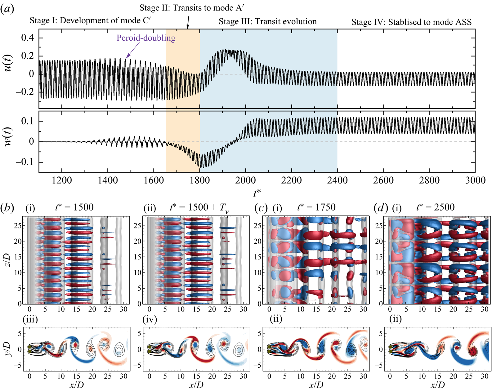
Figure 19. (a) The evolution of streamwise ( $u$) and spanwise velocities (
 $w$) at
  $(x/D, y/D, z/D) = (3, 0, 11.81)$ of the ASS flow at
  $(g^*, {\textit {Re}})= (0.3, 100)$. (b–d) Instantaneous flow fields in the
  $x$–
$x$– $z$ plane (top) and a slice at
  $z/D = 12.5$ (bottom). Isosurfaces of
  $\omega _x = \pm 0.1$ (blue and red) and
  $\omega _z = \pm 0.5$ (grey).
5.3.2. Spatio-temporal symmetry of gap shear layers
The spatio-temporal symmetry for mode A $'$, mode C
 $'$ and mode ASS are explored through examining the evolutions of
  $|\omega _z| = 0.5$ isosurfaces coloured by
  $v$ velocity in the gap region (
 $x/D <3$) in figure 20. The striking features are summarised below.

Figure 20. Evolution of gap shear layers over one vortex shedding cycle. (a) Mode A $'$
$'$  $(g^*, {\textit {Re}})= (0.3, 95)$, where
  $T_v = 11.2$; (b) mode C
 $'$
$'$  $(g^*, {\textit {Re}})= (0.3, 100)$, where
  $T_v = 11$; and (c) mode ASS
  $(g^*, {\textit {Re}})= (0.3, 95)$, where
  $T_v = 12$. The evolutions of gap shear layers are represented by
  $|\omega _z| = 0.5$ isosurfaces coloured by
  $v$ velocity contours at
  $x/D <3$.
(i) The flow fields of mode A
$'$ sampled at an interval of $1/2T_v$ ($T_v = 11.2$) (figure 20a) indicate that its gap shear layers are permanently biased towards one of the cylinders along the cylinder span. The periodicity of mode A$'$ is identical to the vortex shedding period in 2-D base flow.(ii) Mode C
$'$ is distinct in its $2T_v$ periodicity of the spanwise structure. As shown by instantaneous fields over $2T_v$ (figure 20b), the $\omega _z$ isosurfaces at two instants that are $1T_v$ apart from each other form opposite waviness with respect to the $y$ axis (see the arrows with the same colours in figure 20b). A close visualisation of flow fields over $2T_v$ confirms that the three vorticity components share the same spatio-temporal symmetry conditions,
(5.7)Note that the\begin{equation} \mbox{Mode C}': \quad \boldsymbol{\omega}(x,y,z,t)=\boldsymbol{\omega}(x,y,z\pm\lambda_z/2,t+T_v). \end{equation}$2T_v$ periodicity of mode C$'$ is revealed on time histories of velocities at a sampling point (the purple arrow in figure 19a) but not on the spanwise-averaged forces. This is because the mode C$'$ pair cancels with each other and the $2T_v$ periodicity can not be identified through spanwise-averaged quantities. Another striking feature is that, even though the spanwise waviness of the gap shear layers fluctuates with the vortex shedding process, the gap flow at different $z$ is permanently biased towards one of the cylinders.(iii) As for mode ASS (figure 20c), the flow through the gap forms significant waviness along the cylinder span and towards
${\pm }y$ directions. The $v$-velocity distributions that differ by 1$T_v$ ($= 12$) are identical, suggesting that mode ASS is periodic in each vortex shedding period. The flow fields sampled at an interval of $1/8T_v$ over 1$T_v$ indicate that this wave-like pattern is time independent. The spatio-temporal symmetry along the spanwise direction can be described by
(5.8)where\begin{equation} \mbox{Mode ASS:}\quad \boldsymbol{\omega}(x,y,z,t)= \boldsymbol{\omega}(x,-y,z\pm\lambda_z/2,t), \end{equation}$\lambda _z$ has a wavelength around twice of that identified in mode A$'$.


We would like to point out that the nonlinear transition to mode ASS is dependent on the  $L_z$ value adopted in the 3-D DNS. A series of simulations at
  $(g^*, {\textit {Re}})= (0.3, 95)$ and (0.3, 100) with
  $L_z$ varying from 7 to 42 were conducted to investigate this dependence. We found that mode ASS is reproduced only when
  $L_z$ is larger than twice of the
  $\lambda _z$ for mode A
 $'$ (
$'$ ( $L_z \gtrapprox 14D$). We suspect that the flow transition to mode ASS is due to the nonlinear interaction of two mode A
 $'$ pairs.
5.3.3. Hysteresis effect
The existence of hysteresis for the fully developed flow, mode ASS, is explored. The hysteresis effect is first assessed through the Landau model (Landau & Lifshitz Reference Landau and Lifshitz1976) using the case at  $(g^*, {\textit {Re}})= (0.3, 95)$ where the flow is unable to achieve mode ASS. The Landau equation, which considers the evolution of perturbation amplitude
  $A(t)$, is written as
 \begin{equation} \mathrm{d}A/\mathrm{d}t = (\sigma+{\rm i}\omega)A-l(1+{\rm i}c)|A|^2 A+\cdots, \end{equation}
where  $\sigma$ and
  $\omega$ represent the linear growth rate and angular oscillation frequency of the perturbation;
  $c$ is the Landau constant. The sign of
  $l$, which defines the bifurcation nature of a transition, can be determined by the plot of
  $\mathrm {d}\log |A|/\mathrm {d}t$ over
  $|A|^2$, where the slope of the curve at
  $|A|^2 \sim 0$ gives the
  $-l$. The transition is supercritical (non-hysteresis) and subcritical (hysteresis) if
  $l>0$ and
  $l<0$, respectively. More details of this method can be found in Carmo et al. (Reference Carmo, Sherwin, Bearman and Willden2008, Reference Carmo, Meneghini and Sherwin2010) and Jiang & Cheng (Reference Jiang and Cheng2020). In the present case the evolution of
  $|A|$ is measured using the envelope of spanwise velocity
  $w$ at a point
  $(x/D, y/D, z/D) = (3, 0, 14.875)$ in a stage where mode A
 $'$ is developing, stage I shown in figure 17(a). The curve of
  $\mathrm {d}\log |A|/\mathrm {d}t$ over
  $|A|^2$ in figure 21(b) shows a positive slope close to the
  $y$ axis (
 $l>0$), suggesting that mode ASS is subcritical in nature.
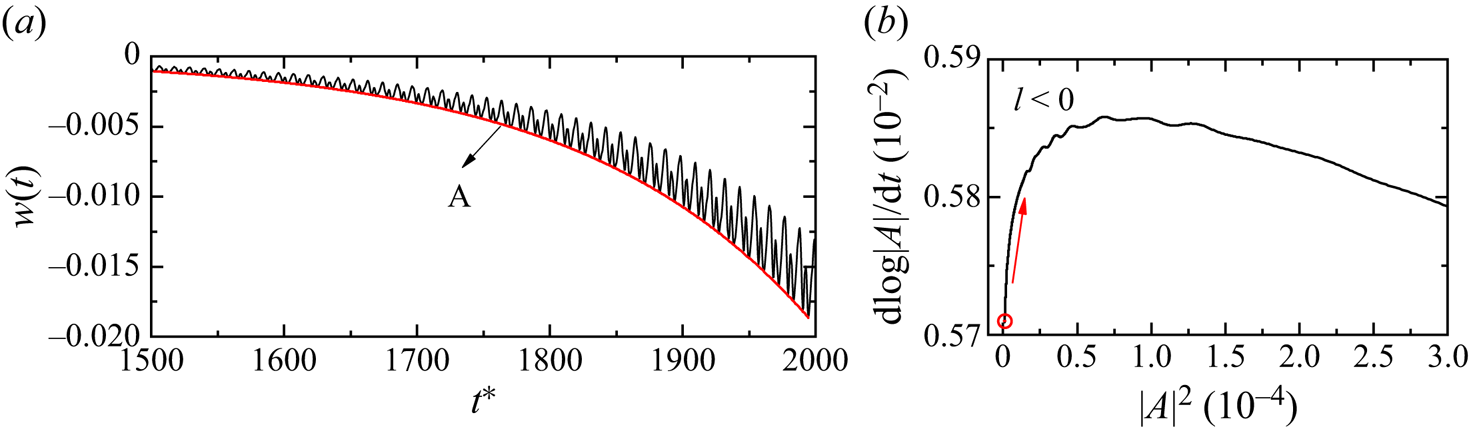
Figure 21. The examination of the hysteresis effect for the flow at  $(g^*, {\textit {Re}})= (0.3, 95)$. (a) A zoomed-in view of
  $w(t)$ in figure 17(a) at
  $t^* = 1500\unicode{x2013} 2000$, where the envelope of
  $w(t)$,
  $A$, are shown as the solid red line. (b) The derivative of the amplitude logarithm over the square of the amplitude, suggesting a subcritical transition (
 $l<0$).
This subcritical transition nature is further confirmed through 3-D DNS at  $g^* = 0.3$ by initialising the flow from the following three ICs.
(1) Initial condition
$Re_H$ (IC-$Re_H$): the flow is initialised from a fully developed 3-D flow at $Re = 95$ (in mode ASS at the time instant shown in figure 17) and gradually increases $Re$ by an interval of $\Delta Re = 5$ until a 2-D wake is developed.(2) Initial condition
$Re_L$ (IC-$Re_L$): the flow is initialised from a 2-D flow at $Re = 85$ and gradually increases $Re$ by an interval of $\Delta Re = 5$ until $Re = 95$.(3) Initial condition 2-D (IC-2-D): the flow is initialised from a 2-D state at the corresponding
$Re$.


The distributions of 2-D and 3-D wakes for the above three ICs are marked as discrete symbols in figure 22. The arrows on the IC- $Re_L$ and IC-
 $Re_H$ branches indicate the directions of successive initialisation. The wake is deemed a 3-D wake first by assessing the
  $\varepsilon _{xy}/\varepsilon _t > 0.001$. Figure 22 shows that three IC branches have different lower-bound
  ${\textit {Re}}$ values for the onset of wake three-dimensionality, forming a hysteresis loop. Precisely, the IC-2-D and IC-
 $Re_L$ both transit at
  ${\textit {Re}} \approx 87.5$ that agree well with the marginal curve estimated by Floquet analysis (
 ${\textit {Re}}_{cr-1} = 87.12$), while the flow remains a 3-D flow till
  ${\textit {Re}} = 80$ for cases with IC-
 $Re_H$ due to the large perturbation introduced by the mode ASS flow. The hysteresis loop observed here confirms the subcritical transition identified from the Landau equation.

Figure 22. Comparisons of the wake state distributions at  $g^* = 0.3$ by initialising the flow from different ICs. The 2-D and 3-D wakes are represented by horizontal lines. The thick grey line indicates the presence of a wake state based on 3-D DNS using a 2-D state at the corresponding
  $Re$ (IC-2-D). The orange and blue solid lines denote the dominance of wake states based on 3-D DNS initialised by a fully developed flow field from adjacent higher
  ${\textit {Re}}$ (IC-
 ${\textit {Re}}_{H}$) and lower
  ${\textit {Re}}$ (IC-
 ${\textit {Re}}_{L}$) values, respectively. The stating points and directions for successive initialisation are marked by the solid star symbols and arrows, respectively.
5.4. Bistable states
In this subsection we examine if the 2-D bistabilities exist when flow develops into 3-D flow. The flow in the bistable IP/FF region is first assessed through both Floquet analysis of IP periodic base flow and 3-D DNS with 2-D FF and IP flows as ICs, denoted as IC-FF and IC-IP, respectively. As displayed in figure 5, the FF flow is unstable to mode FW in the confined region bounded by solid blue and dashed grey lines. Both 3-D DNS with IC-IP and Floquet analysis of the IP base flow at  $(g^*, {\textit {Re}}) = (1.5, 60)$ suggest the IP flow in this specific region is two dimensional. This outcome confirms the physical existence of flow bistability between 3-D mode FW and 2-D IP. For the flows in bistable IP/AP at
  $g^* = 1.2\unicode{x2013} 2.0$, where two cylinder wakes can be either IP or AP, the Floquet analysis identifies multiple bistabilities between 2-D and 3-D flows and among different types of 3-D modes. For examples, the flow in between
  ${\textit {Re}}_{cr-1} - g^*$ lines of mode A-IP and mode A-AP manifests a bistability between 2-D IP and mode A-AP; the flow beyond the marginal curve of
  ${\textit {Re}}_{cr-2} - g^*$ for mode B-AP has a bistability between mode B-AP and mode A-IP. Other bistable states, such as, mode A-IP/mode A-AP, mode B-IP/mode A-AP, can also be observed in 3-D DNS using different ICs.
The developments of the above-mentioned bistabilities are because the wake interference of 2-D flow state has a different influence on the 3-D instabilities. For instance, the occurrence of mode FW at  ${\textit {Re}} \sim 60$ is associated with the wake irregularity in FF flow. The 3-D instability of IP flow, in contrast, is triggered by the elliptical instability of primary vortex cores in IP when
  ${\textit {Re}}$ reaches
  ${\sim }180$. The large difference of
  ${\textit {Re}}_{cr-1}$ for FF flow and IP flow constitutes the bistability here. Similar explanations apply to the multiple bistabilities in the bistable IP/AP region.
6. Discussion
6.1. Wake transitions to 3-D in ASS and FF flows
Two of the salient features of 3-D wake transitions from the ASS and FF base flows observed in figure 5 are (1) the values of  ${\textit {Re}}_{cr-1}$ are considerably lower than their isolated cylinder counterpart and (2)
  ${\textit {Re}}_{cr-1}$ decreases with increasing
  $g^*$. We attributed feature (1) to the asymmetric wake of the ASS base flow and the irregular vortex shedding of the FF flow, and feature (2) to the increasing levels of asymmetry in the ASS base flow (e.g. figure 9) and the irregularity in the FF base flow (e.g. figure 12) with
  $g^*$. Since the transitions to the 3-D mode from ASS and FF flows are subcritical in nature,
  ${\textit {Re}}_{cr-1}$ is expected to be dependent on the level of disturbances present in the flow fields, regardless of the sources of the disturbances. The above inferences seem to be plausible based on the regime map shown in figure 5. For example, the non-overlapping lower
  ${\textit {Re}}$ boundary of the ASS flow regime and the
  ${\textit {Re}}_{cr-1}$ boundary of the ASS base flow do suggest that the wake transition to 3-D flow occurs only when the level of flow asymmetry exceeds a certain level. The overlapping of the
  ${\textit {Re}}_{cr-1}$ boundary of the FF base flow with the lower
  ${\textit {Re}}$ boundary of the irregular FF flow regime may not be a coincidence. We do admit that the above inferences are largely based on simple correlations of flow asymmetry and irregularity with
  $g^*$. It is desirable that vigorous local stability analysis can be conducted to affirm the inferences in future.
6.2. Flow regime classification: 2-D versus 3-D flow
The influence of 3-D flow on the flow regimes classified through a 2-D approach is addressed in this subsection. We are particularly interested in the parameter space covered by the SS, ASS and FF flows at  $g^* < 1.2$ and
  ${\textit {Re}} < \sim 150$, where the 3-D instabilities occur at extremely small
  ${\textit {Re}} \sim 60$. The examination is performed by comparing the flow regimes obtained in 3-D DNS, which utilise fully developed 2-D flows as ICs (cases are marked as discrete circles in figure 5). Generally, the flow regimes identified in 3-D simulations are almost identical to those quantified through 2-D simulations; see, for instance, the following.
(1) At
${\textit {Re}} = 100$ and $g^* = 0.1\unicode{x2013} 1.3$, both 2-D and 3-D simulations identify the regime transition of ‘SS $\to$ ASS $\to$ FF $\to$ IP’. The critical $g^*$ of regime transitions identified through 3-D simulation match well with those identified through 2-D simulations.(2) At
$g^* = 1.0$ and ${\textit {Re}} = 66\unicode{x2013} 100$, where the FF flow develops, the 3-D flows have the same synchronisation states as their 2-D counterparts, as shown in figure 11.


Uncertainty in regime classifications may exist in the vicinity between ASS and FF flow state transitions. As indicated in table 2, the FF flow at  $g^* = 0.3$ and
  ${\textit {Re}} = 110\unicode{x2013} 150$ transitions back to mode ASS in the 3-D simulation.
Table 2. Flow states distribution of two side-by-side cylinders at  $g^* = 0.3$ through 2-D and 3-D simulations. The 3-D simulations use instantaneous 2-D flow states at corresponding
  ${\textit {Re}}$ as ICs.
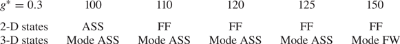
6.3. Existence of other 3-D modes
The present study is primarily focused on the onset transition to 3-D modes under different 2-D wake interference. Periodic base flows such as ASS, IP and AP flows do manifest the second 3-D mode in Floquet analysis. However, over the investigated  ${\textit {Re}}$ range, the second 3-D modes of SS and FF flows are not predicted. In addition, the investigation on the third unstable mode (mode QP) at high
  ${\textit {Re}}$, which is expected to be observed in the IP and AP states, is not comprehensive. Discussions related to the possible existence of these two flows are given below.
To seek the existence of the second 3-D mode in SS flow, 3-D DNS simulations are performed for a case at  $(g^*, {\textit {Re}}) = (0.2, 100)$, where the SS wake is developed in 2-D DNS. The 3-D DNS does observe the occurrence of another type of 3-D structure that is similar to the mode B instability of an isolated circular cylinder. One possibility is that the critical
  ${\textit {Re}}$ for the onset of the second 3-D mode estimated by the Floquet analysis exceeds the maximum
  ${\textit {Re}} = 400$ investigated in this study. Since the existence of one type of 3-D mode destabilises the other due to the nonlinear interactions, it is expected to observe a 3-D mode with a much finer spanwise structure (mode B) at such a low
  ${\textit {Re}}$ in DNS but not in Floquet analysis. The other is likely due to the particular geometry formed by two closely placed side-by-side cylinders, where the secondary vortex street is formed in the near wake of SS at high
  ${\textit {Re}}$. The formation of a secondary vortex street breaks the periodicity of the SS base flow, making it unsuitable for the Floquet analysis. Related studies of flow past two cylinders at a small gap distance also reported only one type of 3-D instability (Carmo et al. Reference Carmo, Meneghini and Sherwin2010; Choi & Yang Reference Choi and Yang2013; Behara, Chandra & Prashanth Reference Behara, Chandra and Prashanth2022). Similarly, the second 3-D mode for the FF flows is not explored in 3-D DNS due to its irregular wake characteristics. We would expect their occurrence according to the knowledge from an isolated cylinder. No further investigation is carried out to explore them.
Only an approximate boundary for the mode QP of IP base flows is provided (the dashed black line in figure 5). The present study is not able to predict the onset boundary for the AP flow. One primary reason is that the base flow becomes marginally periodic when the secondary vortex street develops at large  ${\textit {Re}}$ (Jiang & Cheng Reference Jiang and Cheng2019). Such an example is shown in figure 23(a), where the onset of transition to the secondary vortex street is observed at
  $x/D \approx 20$. Using this flow as the base flow results in an energetic unstable mode originating from the two-layered structure or the secondary vortex street. Attempts were made to artificially shorten the outflow domain size to eliminate this influence. Unfortunately it did not improve the periodicity of the base flow. As an example, the breaking of the reflection symmetry occurs in the AP base flow with an outflow length of
  $20D$ at
  $(g^*, Re) = (1.5, 350)$ (as shown in figure 23b), possibly due to the strong outflow boundary condition (
 $\partial u/\partial x = 0, \partial v/\partial x = 0$). As a result, the wake loses the periodicity in each cycle, making it unsuitable for Floquet analysis.
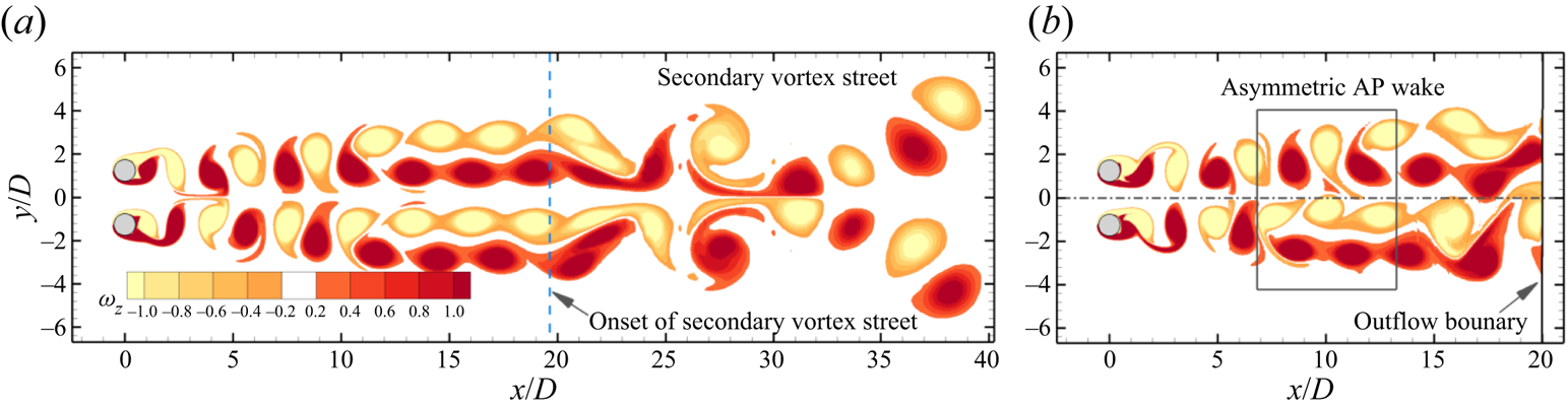
Figure 23. Instantaneous vorticity fields of an AP base flow at  $(g^*, Re) = (1.5, 350)$ for an outflow length of (a) 100
 $D$ and (b) 20
 $D$.
$D$.
We speculate that the Floquet analysis cannot predict the accurate transition boundary for 3-D modes occurring after the first 3-D mode. This speculation is based on the fact that the onset  ${\textit {Re}}$ value of the mode B instability obtained through Floquet analysis (
 ${\textit {Re}} \approx 259$) is considerably higher than that determined by physical experiments (e.g. Williamson Reference Williamson1996b) and numerical studies (e.g. Jiang et al. Reference Jiang, Cheng, Draper, An and Tong2016) for an isolated cylinder. The
  ${\textit {Re}}_{cr-2}-g^*$ boundaries presented in figure 5 may not be exactly the same as those obtained through 3-D DNS. In addition, the third 3-D mode, mode QP, of an isolated cylinder has not been identified in either DNS or experiments at corresponding
  $Re$ (Leontini et al. Reference Leontini, Lo Jacono and Thompson2015). For reasons mentioned above, we do not spend much effort in investigating 3-D modes other than the first 3-D mode.
7. Conclusions
The 3-D wake transitions of steady flow past two identical circular cylinders in a side-by-side arrangement are investigated over the range of gap ratio  $g^*$ from 0.1 to 3.5 and Reynolds number
  ${\textit {Re}}$ up to 400. The critical
  ${\textit {Re}}$ for the first and second 3-D modes, i.e.
  ${\textit {Re}}_{cr-1}$ and
  ${\textit {Re}}_{cr-2}$, and corresponding wavelength, i.e.
  $\lambda _{cr-1}$ and
  $\lambda _{cr-2}$, are quantified through the Floquet analysis, based on five periodic flows: the symmetric single bluff-body wake (SS), asymmetric single bluff-body wake (ASS), biased IP vortex shedding wake (
 $\textrm {IP}_B$), IP vortex shedding wake and AP vortex shedding wake. The onset
  ${\textit {Re}}_{cr-1}$ of the 3-D FF wake is determined using the 3-D DNS. The 3-D wake transition of each type of base flow is summarised below.
(i) At
$g^* \lessapprox 0.25$ in the SS state, the ${\textit {Re}}_{cr-1}$ is more than halved, while the wavelength $\lambda _{cr-1}$ is doubled in comparison with those of a single-cylinder case, which is due to the fact that the effective length scale of the cylinder cluster at small $g^*$ is approximately two times its isolated cylinder counterpart. The wake transits in a sequence of ‘2-D $\to$ mode A’ at increasing ${\textit {Re}}$. With the increase of $g^*$ in the SS flow, the increased flow rate through the gap and the weakening of cluster shear layers around the cylinders delay the initiation of the 3-D instability to higher ${\textit {Re}}$.(ii) When the base flow is in the ASS state, the first 3-D mode (mode A
$'$) occurs at extremely low ${\textit {Re}}$ and the $Re_{cr-1}$ decreases from 100 to 60 as $g^*$ increases from around 0.25 to 0.60. The subharmonic mode C$'$ is found as the second 3-D mode at higher ${\textit {Re}}$ in Floquet analysis. It is demonstrated that the level of asymmetry of the base flow and the flow rate through the gap, which increased with increasing $g^*$, constitutes the occurrence of mode A$'$ and the reduced trends of ${\textit {Re}}_{cr-1}$ and ${\textit {Re}}_{cr-2}$ with $g^*$. The 3-D DNS shows that both mode A$'$ and mode C$'$ are transient features and the flow eventually saturates into an ordered 3-D mode (mode ASS) due to nonlinear effects. The gap flow of mode ASS is characterised by a time-independent waviness structure that is deflected towards $\pm y$ directions along the cylinder span. The wavelength of the waviness structure is around twice the characteristic length scale of a mode A$'$ pair.(iii) At the intermediate
$g^*$ ($\approx 0.6\unicode{x2013} 1.8$) range, where the FF flow develops, the ${\textit {Re}}_{cr-1}-g^*$ curve does not monotonically link the boundaries at both $g^*$ ends. In contrast, it experiences a step jump from ${\sim }65$ to ${\sim }75$ when the base flow changes from ASS to FF at the onset. Further increasing $g^*$, the 3-D mode of FF is destabilised to lower ${\textit {Re}}$. We found that the bifurcation here is prone to irregularity in the two wakes of the FF flow. The 3-D mode of the FF state, referred to as ‘mode FW’, manifests flapping over of 3-D structures intermittently between two wakes. The spanwise characteristic length scale of mode FW decreases monotonically in the streamwise direction along the wake centreline and reduces with increasing ${\textit {Re}}$.(iv) The 3-D transitions on IP and AP coupled wakes at large
$g^* > 1.2$ are similar to their single-cylinder counterparts with mode A as the most unstable mode and mode B as the second 3-D mode at higher ${\textit {Re}}$. Owing to the wake coupling, the mode topology changes, leading to mode A and mode B to bifurcate at smaller and larger ${\textit {Re}}$ values than their single-cylinder counterparts, respectively. The differences from their single-cylinder counterparts reduces with increasing $g^*$.(v) The bistabilities between 2-D and 3-D flows or among 3-D flows are observed in two regions, which is affected by the distinct wake interactions of base flows.


Funding
This work was supported by the Australia Research Council Discovery Grant (Project ID: DP200102804). This research was supported by computational resources provided by the National Computational Merit Allocation Scheme (NCMAS) and the Pawsey Supercomputing Centre with funding from the Australian Government and the Government of Western Australia. C. Ren would like to acknowledge the support from Dalian University of Technology and China Scholarship Council for conducting part of this work while she was a visiting PhD student at the University of Western Australia.
Declaration of interests
The authors report no conflict of interest.
Appendix A
A comprehensive summary of the critical  ${\textit {Re}}$ wavelength
  $\lambda$ and wake interference on 3-D transitions for flow past two side-by-side cylinders is given in table 3.
Table 3. Transition behaviour for two side-by-side circular cylinders.
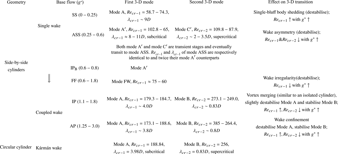
Appendix B
Comparisons of  $\lambda _{z,m}$ over
  $x/D$ for a case at
  $(g^*, Re) = (1.0, 80)$, calculated based on
  $\omega _y \approx \partial u/\partial z$ and
  $\omega _y = \partial u / \partial z - \partial w/\partial x$, are performed. Figure 24 indicates that the approximation of using
  $\omega _y \approx \partial u/\partial z$ introduces a smaller
  $\lambda _{z,m}$ compared with the actual
  $\omega _y$. The variations of
  $\lambda _{z,m}$ with respect to
  $x/D$, however, are similar by using different components.
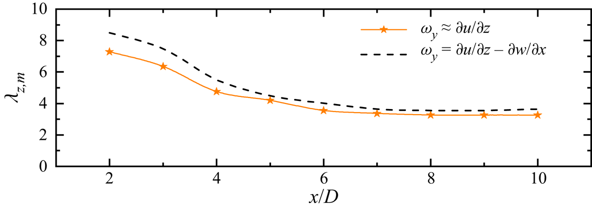
Figure 24. Distributions of the most probable spanwise wavelength,  $\lambda _{z,m}$, with respect to
  $x/D$ for a mode FW at
  $y/D = 0$. The
  $\lambda _{z,m}$ is calculated based on an approximation of
  $\omega _y \approx \partial u / \partial z$ (the solid orange line with stars) and
  $\omega _y = \partial u / \partial z - \partial w/\partial x$ (the dashed black line) using (5.4) and (5.5).


 Open access