


1. Introduction
Turbulence is ubiquitous in the stably stratified ocean, where it facilitates the vertical mixing of water masses, thus playing a vital role in determining global transport of scalars such as heat, carbon and nutrients (Ivey, Winters & Koseff Reference Ivey, Winters and Koseff2008; Talley et al. Reference Talley2016). Observational estimates of small-scale turbulence quantities may be obtained using measurements of fluctuating density (or temperature, assuming a linear equation of state for a single dynamic scalar) and velocity fields captured by microstructure profilers, small probes that descend vertically through a column of water to depths of up to 6000 m and that have been deployed across much of the ocean (Waterhouse et al. Reference Waterhouse2014). The primary quantities of interest for diagnosing mixing rates are the rate of dissipation of density variance  $\chi$ and the rate of dissipation of turbulent kinetic energy
  $\varepsilon$ (defined below). Calculating precise values of
  $\varepsilon$ and
  $\chi$ requires that nine spatial derivatives of velocities and three spatial derivatives of density be resolved simultaneously, and so in practice theoretical ‘surrogate’ models are commonly invoked which require only derivatives in a single coordinate direction (typically the vertical). Our focus here is on estimating
  $\varepsilon$ and
  $\chi$ given exact values of these vertical derivatives alone as notionally measured by an idealised microstructure profiler. This facilitates a study of the underlying stratified turbulence dynamics and is a step toward improved mixing parameterisations ‘output’ from ocean measurement ‘inputs’, although it does not address other causes of uncertainty in obtaining accurate and robust in situ measurements of
  $\varepsilon$ and
  $\chi$, due for example to uncertainties in the mapping between the raw measurements and the vertical gradients of velocity and density (Gregg et al. Reference Gregg, D'Asoro, Riley and Kunze2018).
The majority of models for  $\varepsilon$ and
  $\chi$ are based on the fundamental assumption that turbulence is homogeneous and isotropic at small scales, although there have been efforts to model dissipation in stratified turbulence by use of a suitable proxy that captures the modifying influence of the stratification (Weinstock Reference Weinstock1981; Fossum, Wingstedt & Reif Reference Fossum, Wingstedt and Reif2013). We appeal to modern data-driven tools to supplement and extend existing theoretical models for
  $\varepsilon$ and
  $\chi$ in the anisotropic stratified turbulent regime. Data-driven methods have become popular for the modelling of fluid flows due to their inherent ability to capture complex spatio-temporal dynamics (Salehipour & Peltier Reference Salehipour and Peltier2019; Brunton, Noack & Koumoutsakos Reference Brunton, Noack and Koumoutsakos2020) and reveal insights into flow physics (Callaham et al. Reference Callaham, Koch, Brunton, Kutz and Brunton2021; Couchman et al. Reference Couchman, Wynne-Cattanach, Alford, Caulfield, Kerswell, MacKinnon and Voet2021). They are also seeing widespread use for closure modelling, for example improving sub-grid parameterisation schemes in simulations of turbulence (Maulik et al. Reference Maulik, San, Rasheed and Vedula2019; Portwood et al. Reference Portwood, Nadiga, Saenz and Livescu2021; Subel et al. Reference Subel, Chattopadhyay, Guan and Hassanzadeh2021) and large-scale models of the atmosphere and ocean (Rasp, Pritchard & Gentine Reference Rasp, Pritchard and Gentine2018; Bolton & Zanna Reference Bolton and Zanna2019). Bayesian models that can provide uncertainty estimates as opposed to standard deterministic predictions are appealing in these settings as they give an important measure of model reliability and can accurately reproduce higher-order moments of a distribution of values over a set of data (Maulik et al. Reference Maulik, Fukami, Ramachandra, Fukagata and Taira2020; Barnes & Barnes Reference Barnes and Barnes2021; Guillaumin & Zanna Reference Guillaumin and Zanna2021).
Deep neural network models for determining the relationship between physical observables can be essentially described as the substitution of an equation whose functional form and accompanying parameters are based on known physical constraints for an equation whose functional form is determined by optimising an extremely large number of parameters using data obtained from measurements of the system: this results in what is commonly referred to as a ‘black-box algorithm’. In cases where the underlying physical processes are not fully understood, or not fully representable using a limited subset of system observables, these deep learning methods often result in greatly improved accuracy over traditional physics-based methods. This is, however, at the expense of generalisability to data from similar but distinct systems, where knowledge of how the underlying physics is encoded into a traditional theoretical model can be used to adapt it. Since they consist of such a large number of parameters – leaving the physics somewhat intractable – it is not obvious how to adapt deep learning models in the same way. To try to overcome this difficulty, either some information about the physics can be encoded into the architecture of the model a priori (such models are often referred to as ‘physics-informed’) (Ling, Kurzawski & Templeton Reference Ling, Kurzawski and Templeton2016; Zanna & Bolton Reference Zanna and Bolton2020; Beucler et al. Reference Beucler, Pritchard, Rasp, Ott, Baldi and Gentine2021), or a highly general model can be analysed a posteriori to ‘discover’ physically relevant features (Toms, Barnes & Ebert-Uphoff Reference Toms, Barnes and Ebert-Uphoff2020; Portwood et al. Reference Portwood, Nadiga, Saenz and Livescu2021).
Since exact observational measurements of  $\varepsilon$ and
  $\chi$ are not feasible at present for testing our methodology, we consider direct numerical simulations (DNS) of stably stratified turbulence (SST) as a model flow for the turbulence length and time scales of the ocean, the relevance of which is supported by a modest but increasing body of observations (Riley & Lindborg Reference Riley and Lindborg2008). Broadly, such flows can be characterised by suitable Reynolds and Froude numbers,
  $Re_h$ and
  $Fr_h$, as well as the Prandtl number
  $Pr$, defined here as
 \begin{equation} Re_h= \frac{U_hL_h}{\nu},\quad Fr_h=\frac{U_h}{L_h N},\quad Pr=\frac{\nu}{\kappa}. \end{equation}
Here,  $U_h$ and
  $L_h$ are horizontal velocity and length scales,
  $N$ is a characteristic buoyancy frequency associated with the ambient stratification,
  $\nu$ is the kinematic viscosity and
  $\kappa$ is the thermal diffusivity. The SST regime is then a turbulent flow regime where buoyancy effects due to the presence of a background density stratification have a leading-order influence on the flow, which corresponds to
  $Re_h\gg 1$ and
  $Fr_h \lesssim 1$. As
  $Fr_h$ decreases below
  $O(1)$, horizontal motions tends to decouple into thin vertical layers with large horizontal extent, with the resulting vertical shearing being an important mechanism for generating turbulence (Lilly Reference Lilly1983). The resulting ‘pancake’ layers are predicted to evolve with vertical length scale
  $U_h/N$ (Billant & Chomaz Reference Billant and Chomaz2001), a behaviour that has been observed in experiments (e.g. Lin & Pao Reference Lin and Pao1979; Spedding Reference Spedding1997), as well as in both forced and freely decaying DNS (e.g. Riley & de Bruyn Kops Reference Riley and de Bruyn Kops2003; Brethouwer et al. Reference Brethouwer, Billant, Lindborg and Chomaz2007).
The SST regime exhibits anisotropy across a range of scales (Lang & Waite Reference Lang and Waite2019), the largest of which is set by the vertical layered structure described above and whose existence is predicted by the value of  $Fr_h$. Whether anisotropy persists at the smallest scales of motion (sometimes referred to as return to isotropy; Lumley & Newman Reference Lumley and Newman1977), thus affecting the way in which models for
  $\varepsilon$ and
  $\chi$ depend on individual velocity and density derivatives, depends on the existence of an inertial range between these scales and the length scale of motion below which eddies evolve without being influenced by the stratification (Gargett, Osborn & Nasmyth Reference Gargett, Osborn and Nasmyth1984). For the velocity field, the breadth of the inertial range is characterised by an emergent Reynolds number, which for stratified flows is most commonly defined as the buoyancy Reynolds number
 \begin{equation} Re_b := \frac{\varepsilon}{\nu N^2}. \end{equation}
 If  $Re_b \ll 1$, scaling arguments and simulation results indicate that
  $\varepsilon$ will be dominated by vertical shear (Riley, Metcalfe & Weissman Reference Riley, Metcalfe and Weissman1981; Godoy-Diana, Chomaz & Billant Reference Godoy-Diana, Chomaz and Billant2004; de Bruyn Kops & Riley Reference de Bruyn Kops and Riley2019). On the other hand, when
  $Re_b\gg 1$ and turbulence is locally almost isotropic, one can appeal to symmetry arguments to relate directly the horizontal and vertical spatial derivatives of velocity and density, thus simplifying the expression for
  $\varepsilon$ and
  $\chi$ (see e.g. Pope Reference Pope2000). Several numerical studies quantify the degree of small-scale isotropy in SST as a function of
  $Re_b$ (Hebert & de Bruyn Kops Reference Hebert and de Bruyn Kops2006; de Bruyn Kops Reference de Bruyn Kops2015) from which we conclude that SST will be close to isotropic at the small scales if
  $Re_b \approx 50$ or larger. Importantly, there are many regions of the ocean in which it is estimated
  $Re_b < 50$ (e.g. Moum Reference Moum1996; Jackson & Rehmann Reference Jackson and Rehmann2014; Scheifele et al. Reference Scheifele, Waterman, Merckelbach and Carpenter2018), with potentially significant consequences for the accuracy of isotropic models for
  $\varepsilon$. When
  $Pr>1$, density fluctuations are expected on smaller scales than those of velocity leading to the emergence of a viscous–convective subrange. Nonetheless, it may still be argued that the isotropic inertial range in the density field has the same high wavenumber cutoff as that of the velocity field (Batchelor Reference Batchelor1959), and thus the breadth is again governed by
  $Re_b$. We note that technically even for
  $Re_b\gg 1$ the scalar derivatives cannot be exactly isotropic if there is a mean gradient (Warhaft Reference Warhaft2000), although this detail will not be of practical importance for our purposes here. When only measurements of the density field are available, the buoyancy Reynolds number is sometimes replaced by the parameter
  $Pr^{-1} Cx$, where
 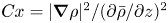 $Cx = |\boldsymbol {\nabla } \rho |^2/(\partial \bar {\rho }/\partial z)^2$ is the Cox number for a flow with turbulent density fluctuations
  $\rho$ about a background density profile
  $\bar {\rho }(z)$ (Dillon & Caldwell Reference Dillon and Caldwell1980).
Mean values of  $\varepsilon$ and
  $\chi$ can be accurately computed from single velocity and scalar derivatives if, by some method, the anisotropy in the velocity and scalar fields is known. This is the basis of the majority of existing models, e.g. estimating the dissipation rates by assuming isotropy. In practice, since
  $Re_b$ itself depends on
  $\varepsilon$, it is not possible to diagnose precisely a turbulent regime given a limited subset of derivatives of velocity and density. Moreover, while the mean dissipation rates may be accurate based on assumptions of isotropy, the distribution of local values
  $\varepsilon _0$ and
  $\chi _0$ (hereafter differentiated from appropriately averaged mean values
  $\varepsilon$ and
  $\chi$ using a subscript
  $0$) will not be. Using simulations of almost perfectly homogeneous isotropic turbulence, Almalkie & de Bruyn Kops (Reference Almalkie and de Bruyn Kops2012b) show that the probability density function (p.d.f.) of any of the velocity derivatives have nearly exponential left tails rather than the approximately log-normal tail assumed by Kolmogorov (Reference Kolmogorov1962) for the local dissipation rate, that is actually also widely observed in simulation data.
Motivated by the discussion above, in this work our primary aim will be to build highly general models for estimating local ( $\varepsilon _0, \chi _0$) and mean values (
 $\varepsilon,\chi$) of the dissipation rates, that can make accurate predictions across a range of turbulent regimes described by different values of
  $Re_b$. We construct and train a probabilistic convolutional neural network (PCNN) model to compute local values of dissipation
  $\varepsilon _0$ and
  $\chi _0$ within vertical fluid columns, motivated by available observational data collected by microstructure profilers. The architecture of the model is constructed based on the fundamental physical arguments that vertical gradients of velocity and density should be strongly correlated and of leading-order importance for determining local dissipation rates in stratified turbulence, crucially both locally and non-locally (for example, whether or not a particular region of fluid supports energetic turbulence is likely to depend at least on the local shear as well as some surrounding background density gradient) (Caulfield Reference Caulfield2021). The probabilistic component is included based on the emerging importance of accurately predicting the tails of the distributions of values of small-scale mixing properties (Cael & Mashayek Reference Cael and Mashayek2021; Couchman et al. Reference Couchman, Wynne-Cattanach, Alford, Caulfield, Kerswell, MacKinnon and Voet2021).
The data-driven models may be used as an effective tool revealing the fundamental limitations of theoretical models for local stratified turbulent flow properties derived based on global statistics. For this purpose, it will be important to compare the data-driven models with strict benchmarks whose functional form incorporates as many of the currently known fluid dynamical constraints as possible. Therefore we also propose new empirically derived theoretical models for calculating  $\varepsilon _0$ and
  $\chi _0$ using the same inputs based on the knowledge that the local isotropy of the flow is primarily determined by the buoyancy Reynolds number
  $Re_b$, which here serve as a helpful baseline to compare with the deep learning model, but may also be considered practical substitutes for isotropic models in their own right. A comparison between the theoretical and PCNN models provides some interesting insights into the limitations of using mean quantities rather than local information for predicting mixing properties of stratified turbulent flows. Moreover, we analyse the structure of the optimised deep learning models to attempt to interpret which features give rise to improvements in accuracy over physics-based theoretical models.
To achieve our primary aim, the remainder of this paper is organised as follows. In § 2 we outline the key features of the DNS used throughout and describe how assumptions of isotropy may be used to construct models for  $\varepsilon$ and
  $\chi$. We also present empirically determined theoretical models for
  $\varepsilon$ and
  $\chi$ based on the value of a suitable proxy for the buoyancy Reynolds number
  $Re_b$, and introduce the probabilistic deep learning model to be evaluated against the theoretical models. Qualitative and quantitative comparisons are shown in § 3, and an analysis and interpretation of the deep learning model is carried out in § 4. We discuss some of the wider implications of the results and conclude in § 6.
2. Methods
2.1. Simulations and theory
Much of the ocean thermocline is believed to be in a ‘strongly stratified turbulence’ regime characterised by large Reynolds number and relatively small Froude number (Moum Reference Moum1996; Brethouwer et al. Reference Brethouwer, Billant, Lindborg and Chomaz2007), defined by (1.1a–c), or in their ‘turbulent’ form by eliminating the horizontal length scale  $L_h$ in favour of a measured turbulent dissipation via the relation
  $\varepsilon = U_h^3/L_h$, as
 \begin{equation} Re_t=U_h^4/(\nu \varepsilon), \quad Fr_t=\varepsilon/(NU_h^2). \end{equation}
For a flow with zero mean shear such as will be considered here,  $U_h$ is taken to be the root mean squared (r.m.s.) velocity and
  $\varepsilon$ is volume averaged over the flow domain. In order to obtain a dataset of stratified turbulence that is broadly representative of a diverse and continuously evolving ocean environment, we appeal to DNS of decaying, strongly stratified turbulence with a large dynamic range accommodating motions on a wide range of spatial scales (de Bruyn Kops & Riley Reference de Bruyn Kops and Riley2019). Simulations are carried out by solving the Navier–Stokes equations with the non-hydrostatic Boussinesq approximation, in the dimensionless form
 $$\begin{gather} \frac{\partial \boldsymbol{u} }{\partial t}+\boldsymbol{u}\boldsymbol{\cdot} \boldsymbol{\nabla} \boldsymbol{u} ={-}\left(\frac{1}{Fr}\right)^2\rho \boldsymbol{e}_z - \boldsymbol{\nabla} p +\frac{1}{Re}\nabla^2\boldsymbol{u}, \end{gather}$$
 $$\begin{gather}\boldsymbol{\nabla} \boldsymbol{\cdot} \boldsymbol{u} = 0, \end{gather}$$
 $$\begin{gather}\frac{\partial \rho}{\partial t} +\boldsymbol{u}\boldsymbol{\cdot} \boldsymbol{\nabla} \rho - w = \frac{1}{Re Pr}\nabla^2 \rho. \end{gather}$$
The dimensionless parameters  $Re$,
$Re$,  $Pr$ and
  $Fr$ are defined by
 \begin{equation} Re = \frac{U_0 L_0}{\nu}, \quad Fr = \frac{U_0}{N L_0},\quad Pr = \frac{\nu}{\kappa}. \end{equation}
Here,  $U_0$ and
  $L_0$ are characteristic (horizontal) velocity and length scales of the flow in its initialised state,
  $\nu$ and
  $\kappa$ are the momentum and density diffusivities and
  $N$ is the (imposed and uniform) background buoyancy frequency. Density is non-dimensionalised using the scale
  $-L_0 N^2\rho _a/g$, where
  $g$ is the acceleration due to gravity and
  $\rho _a$ is a reference density, whilst time is non-dimensionalised using the scale
  $L_0/U_0$. Note that
  $\rho$ is defined as a departure from an imposed uniform background density gradient, so that the total dimensionless density
  $\rho _t$ can be written (up to a constant reference density) as
  $\rho _t = \rho + z$.
Equations (2.2)–(2.4) are solved in a triply periodic domain using a pseudospectral method, with a third-order Adams–Bashforth method used to advance the equations in time and a 2/3 method of truncation for dealiasing fields. Simulations are initialised with the velocity fields in a state of homogeneous, isotropic turbulence. This is achieved by first performing unstratified simulations which are forced to match an empirical spectrum suggested by Pope (Reference Pope2000), using the method described in Almalkie & de Bruyn Kops (Reference Almalkie and de Bruyn Kops2012b). Once suitable conditions have been achieved, a gravitational field is imposed on the density stratification and forcing is switched off, leaving turbulence to decay freely. With the stratification applied, the flow evolves with a natural time scale given by the buoyancy period  $T_B = {2{\rm \pi} / N}$. As discussed by de Bruyn Kops & Riley (Reference de Bruyn Kops and Riley2019), it is often instructive to observe the flow in terms of the number of buoyancy periods
  $T$ after the stratification has been imposed.
The evolution of turbulence and its interaction with the background density stratification is dynamically rich and motions on a variety of length scales emerge which may be used to describe the instantaneous state of the flow. The largest-scale horizontal motions in the flow are described by the integral length scale  $L_h$ calculated here from the r.m.s. velocities using the method described in appendix E of Comte-Bellot & Corrsin (Reference Comte-Bellot and Corrsin1971). This characterises the largest eddies which inject energy into turbulent motions. A turbulent cascade drives this energy down scale until it is dissipated as heat at the Kolmogorov scale
  $L_K$ (or, for the density field, the Batchelor scale
  $L_B$). Two intermediate scales that arise due to the presence of the stratification are the buoyancy scale
  $L_b$ and the Ozmidov scale
  $L_O$. The buoyancy scale is a vertical scale describing the height of the pancake layers that form, whilst the Ozmidov scale describes the size of the largest eddies which are unaffected by the stratification. These length scales are defined as follows:
 \begin{equation} L_K = (\nu^3/\varepsilon)^{1/4},\quad L_B=L_K/Pr^{1/2}, \quad L_b = U_h/N, \quad L_O = (\varepsilon/N^3)^{1/2}. \end{equation}
De Bruyn Kops & Riley (Reference de Bruyn Kops and Riley2019) perform four simulations for various  $Fr$ and
  $Re$ at
  $Pr=1$. Here, we use data from a modified version of the simulation with largest
  $Re$ which has
  $Pr=7$ to be more representative of the ocean in regions where heat is the primary stratifying agent. Further details may be found in Riley, Couchman & de Bruyn Kops (Reference Riley, Couchman and de Bruyn Kops2023). The Froude and Reynolds numbers for the simulation are
  $Fr=1.1$ and
  $Re=2480$. To obtain an appropriate rate of decay of turbulence, the horizontal domain size
  $L_x=L_y$ is chosen to initially accommodate roughly 84 integral length scales
  $L_h$, with the vertical extent
  $L_z=L_x/2$. To resolve motions adequately at the Batchelor scale
  $L_B$, this requires a maximum resolution of
  $N_x=N_y=12\ 880$,
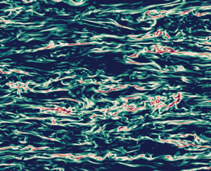
  $N_z=N_x/2$. We take fully three-dimensional snapshots of the velocity and density fields (evenly sparsed by a factor of two in each coordinate direction for computational ease) at various time points
  $T=0.5,1,2,4,6,7.7$ during the flow evolution. This covers an extent of time over which the turbulence decays from being highly energetic and almost isotropic, to a near quasi-horizontal regime in which flow fields have the structure of thin horizontal layers, characteristic of stratified turbulence. The evolution of non-dimensional parameters
  $Fr_h$,
  $Re_h$,
  $Fr_t$,
  $Re_t$ and
  $Re_b$ describing the instantaneous state of the turbulence at each time point are given in table 1.
Table 1. Non-dimensional parameters for the simulation used at various numbers of buoyancy periods  $T$ following the introduction of the stratification. Note at
  $T=0.5$ we have
  $Re_h=Re_0=2480$ and
  $Fr_h=Fr_0=0.175$. Here,
  $\varDelta = L_x/(N_x/2)$ is the grid spacing of the snapshots, which are evenly sparsed by a factor of 2 in each coordinate direction from the DNS resolution.

2.2. Dissipation rates and isotropic models
The local (dimensionless) instantaneous rate of turbulent energy dissipation  $\varepsilon _0$ is defined as
 \begin{equation} \varepsilon_0 = \frac{2}{Re} s_{ij} s_{ij}, \quad s_{ij} = \frac{1}{2}\left(\frac{\partial u_i}{\partial x_j} + \frac{\partial u_j}{\partial x_i}\right), \end{equation}
where the  $u_i$ represent turbulent velocity fluctuations. The corresponding local rate of potential energy dissipation
  $\chi _0$ is defined as
 \begin{equation} \chi_0 = \frac{1}{Re Pr}\left(\frac{1}{Fr}\right)^2\frac{\partial \rho}{\partial x_j}\frac{\partial \rho}{\partial x_j}. \end{equation}
As noted in the introduction, measuring the exact value of  $\varepsilon _0$ and
  $\chi _0$ requires that all spatial derivatives of the velocity and density fields be resolved, a task that is difficult even for laboratory flows, and certainly not possible at present in the context of oceanographic data. Thus it is common to make simplifying assumptions about the turbulence in order to proceed. If one assumes that turbulence is both homogeneous and isotropic, then averaging over some sufficient region, both expressions above can be written in terms of a single derivative. Microstructure profilers usually measure vertical derivatives, hence here we will consider the following isotropic models for
  $\varepsilon _0$ and
  $\chi _0$:
 $$\begin{gather} \varepsilon_0^{{iso}} = \frac{15}{4Re}S^2; \quad S^2 := \left(\frac{\partial u}{\partial z}\right)^2 + \left(\frac{\partial v}{\partial z}\right)^2, \end{gather}$$
 $$\begin{gather}\chi_0^{{iso}} = \frac{3}{Re\,Pr}\left(\frac{1}{Fr}\right)^2\left(\frac{\partial \rho}{\partial z}\right)^2. \end{gather}$$
Here,  $S^2$ is the (squared) local vertical shear. As pointed out by Almalkie & de Bruyn Kops (Reference Almalkie and de Bruyn Kops2012b), these models are exact in the means (which here we take to be a spatial volume average denoted by angle brackets
  $\langle {\cdot } \rangle$) when turbulence is perfectly isotropic, but even in this idealised situation there may be significant differences in the frequency distributions of local values.
2.3. An empirical model
Equations (2.9) and (2.10) are only appropriate (strictly in the mean sense) provided that there exists an inertial range of scales above the Kolmogorov scale  $L_K$ (or equivalently for
  $\chi$, the Batchelor scale
  $L_B$) within which the flow is close to isotropic. Noting that we can write
  $Re_b = (L_O/L_K)^{4/3}$, whether or not such a range exists at small scales is primarily dependent on the value of the buoyancy Reynolds number, making this the most important parameter for determining the accuracy of the isotropic models above. Observational evidence supporting this hypothesis dates back to the measurements of Gargett et al. (Reference Gargett, Osborn and Nasmyth1984), with many recent DNS confirming the agreement with the theory (see, e.g. de Bruyn Kops & Riley Reference de Bruyn Kops and Riley2019; Lang & Waite Reference Lang and Waite2019; Portwood, de Bruyn Kops & Caulfield Reference Portwood, de Bruyn Kops and Caulfield2019). Lang & Waite (Reference Lang and Waite2019) demonstrate that the primary effect of the Froude number
  $Fr_h$ in this context is to control the larger-scale anisotropy. Therefore, even in a strongly stratified flow with
  $Fr_h\lesssim 1$, (2.9) and (2.10) are still expected to be accurate provided
  $Re_b$ is sufficiently large.
When  $Re_b$ becomes small, buoyancy starts to dominate inertia at even the smallest vertical scales, prohibiting the formation of an inertial range. Consequently, the relative magnitudes of the velocity and density derivatives in (2.7) and (2.8) are expected to be substantially different from those predicted by isotropy, eventually being dominated by the vertical derivative terms in the limit
  $Re_b\ll 1$ as demonstrated (at least for
  $\varepsilon$) numerically and experimentally by, e.g. de Bruyn Kops & Riley (Reference de Bruyn Kops and Riley2019), Hebert & de Bruyn Kops (Reference Hebert and de Bruyn Kops2006), Praud, Fincham & Sommeria (Reference Praud, Fincham and Sommeria2005) and Fincham, Maxworthy & Spedding (Reference Fincham, Maxworthy and Spedding1996). Therefore, as suggested by Hebert & de Bruyn Kops (Reference Hebert and de Bruyn Kops2006), it is reasonable to suppose that the ratios
  $\varepsilon /S^2$ and
  $\chi/(\partial \rho/\partial z)^2$ should be a function of
  $Re_b$, giving a natural way of constructing models for
  $\varepsilon$ and
  $\chi$ in stratified flows that take only vertical derivatives of velocity and density as inputs. The caveat of models constructed in this way is is that the additional required input
  $Re_b$ is itself by definition a function of the desired output
  $\varepsilon.$ To circumvent this issue, we appeal to a surrogate buoyancy Reynolds number
 \begin{equation} Re_b^S ={-}Fr^2\frac{\langle S^2\rangle}{\langle \partial \rho_t/\partial z\rangle }, \end{equation}
which at least varies monotonically with  $Re_b$ (and which we note is implicitly invoked via the isotropic assumption when working with observational data).
We wish to derive a local model for  $\varepsilon _0$ and
  $\chi _0$ that now depends on
  $Re_b^S$ as well as
  $S^2$ and
  $\partial \rho /\partial z$. An important subtlety to note is the introduction of some ambiguity in defining a suitable surrogate buoyancy Reynolds number in the local picture due to how the (assumed) spatial averaging in (2.11) is interpreted. Such ambiguities can have appreciable effects on subsequently diagnosed turbulent statistics in stratified flows, as has been discussed by Arthur et al. (Reference Arthur, Venayagamoorthy, Koseff and Fringer2017) and Lewin & Caulfield (Reference Lewin and Caulfield2021). Because it describes anisotropy, which is inherently a non-local flow property, here we assume the ‘true’
  $Re_b^S$ is a bulk value averaged over the domain i.e.
  $Re_b^S = Fr^2\langle S^2\rangle$ (since
  $\langle \partial \rho _t /\partial z\rangle =-1$ by construction). Of course, in the observational setting where measurements are limited, a representative bulk value may be computed by averaging a suitably large section of a vertical profile, over a scale at least as big as the Ozmidov scale
  $L_O$. However, this method may be ineffective when the flow is spatially separated into dynamically distinct regions as discussed by Portwood et al. (Reference Portwood, de Bruyn Kops, Taylor, Salehipour and Caulfield2016). This issue is circumvented by the data-driven model we present in § 2.4, which implicitly ‘learns’ the relevant non-local region of influence on local dissipation rates. With a suitably defined
  $Re_b^S$, we propose the following model:
 $$\begin{gather} \varepsilon_0^{{emp}} = \frac{f(Re_b^S)}{Re} S^2, \end{gather}$$
 $$\begin{gather}\chi_0^{{emp}} = \frac{g(Re_b^S)}{RePrFr^2} \left(\frac{\partial \rho}{\partial z}\right)^2, \end{gather}$$
where  $f(Re_b^S)$ and
  $g(Re_b^S)$ are functions to be determined empirically, based on theoretical constraints. For
  $Re_b^S\gg 1$ the flow is locally isotropic and, in the mean sense, we should have
  $f\to 15/4$,
  $g\to 3$, as in (2.9) and (2.10). For
  $Re_b^S\ll 1$, horizontal diffusion becomes negligible and we therefore have
  $f\to 1$,
  $g\to 1$ (Riley et al. Reference Riley, Metcalfe and Weissman1981; Godoy-Diana et al. Reference Godoy-Diana, Chomaz and Billant2004; de Bruyn Kops & Riley Reference de Bruyn Kops and Riley2019). Data from the decaying turbulence simulation indicate a roughly linear transition from the viscously dominated
  $Re_b^S\ll 1$ regime to the isotropic
  $Re_b^S\gg 1$ regime, as shown in figure 1. Therefore, to match the required asymptotic behaviour and linear transition region, we propose the following models for the dimensionless functions
  $f$ and
  $g$:
$g$:
 $$\begin{gather} f(Re_b^S) = \tfrac{19}{8} + \tfrac{11}{8}\tanh(a\log Re_b^S - b), \end{gather}$$
 $$\begin{gather}g(Re_b^S)= 2 + \tanh(c\log Re_b^S - d). \end{gather}$$
Here, the constants  $b$ and
  $d$ loosely represent the transition value between stratified turbulent and stratified viscous regimes, whilst
  $a$ and
  $c$ characterise the width of the transition region. These can be specified by a simple least-squares optimisation procedure that compares the functional approximations with the DNS data at the values of
  $Re_b^S$ indicated in figure 1: it is found that empirical values of
  $a=1, b=0.8$ and
  $c=d=0.9$ give an extremely close qualitative fit of the empirical function curves with the domain-averaged data, as can be seen in the figure. Note that in general
  $a\neq c$ and
  $b\neq d$ due to the difference in the smallest scales of motion caused by a non-unity Prandtl number
  $Pr=7$, although in practice we see that these differences are relatively small (and largely insignificant).

Figure 1. Values of the ratios (a)  $Re \varepsilon /(\langle S^2\rangle )$ and (b)
  $Re\,Pr\,Fr^2\chi /(\langle \rho _z^2\rangle )$ for different values of the surrogate buoyancy Reynolds number
  $Re_b^S$. Here,
  $Re_b^S$ is computed by interpreting the averaging in (2.11) as over the entire domain. The solid blue lines represent the empirical model functions (2.12) and (2.13), whilst the dashed lines represent the isotropic ratios from (2.9) and (2.10). Black markers represent the true values obtained from domain-averaged DNS quantities. The Jupyter notebook for producing the figure can be found https://www.cambridge.org/S0022112023006791/JFM-Notebooks/files/Fig1/fig1.ipynb.
There have been a limited number of attempts to model the influence of strong anisotropy on dissipation rates  $\varepsilon$ and
  $\chi$. Weinstock (Reference Weinstock1981) proposes a modified model for
  $\varepsilon$ in stratified turbulence that depends on r.m.s. vertical velocities
  $\langle w^2 \rangle$ and the buoyancy frequency
  $N$. Fossum et al. (Reference Fossum, Wingstedt and Reif2013) instead suggest a model for
  $\varepsilon$ in terms of
  $\chi$, pointing out that
  $\chi$ itself may be replaced by vertical density derivatives via a suitable tuning coefficient. To our knowledge, the empirical models (2.12) and (2.13) constitute a first attempt to construct an explicit theoretical model for dissipation rates during the transition of such a flow from a near-isotropic to a buoyancy-dominated regime based on vertical derivatives of velocity and density only. Based on the theoretical scaling arguments discussed above, the functional forms of
  $f$ and
  $g$ are expected to remain independent of flow configuration, with the relevant asymptotic behaviour and linear transition having been observed in a number of previous forced and freely evolving DNS studies, e.g. Lang & Waite (Reference Lang and Waite2019), Brethouwer et al. (Reference Brethouwer, Billant, Lindborg and Chomaz2007) and Hebert & de Bruyn Kops (Reference Hebert and de Bruyn Kops2006). The transition value of
  $Re_b^S$ and width of the transition region represented by the values of
  $a$,
$a$,  $b$,
$b$,  $c$ and
  $d$ also appear to be roughly consistent across studies, although a more detailed investigation would be required to quantitatively verify this. Here, (2.12) and (2.13) serve as useful comparative benchmarks for the data-driven model outlined below that are more strict than the isotropic models (2.9) and (2.10).
2.4. Constructing a data-driven model
2.4.1. Model architecture
Here, we construct a general model for computing local values of  $\varepsilon _0$ and
  $\chi _0$ from measurements of vertical derivatives of velocity and density, without explicitly appealing to arguments that rely on mean averaged quantities used for deriving the theoretical models above. We restrict ourselves to mimicking the oceanographic microstructure scenario where only vertical column measurements are available. To facilitate a comparison between this approach and the explicit theoretical models described above, we allow
  $\varepsilon _0$ to depend on local values of
  $S^2$ and
  $\chi _0$ to depend on local values of
  $(\partial \rho /\partial z)^2$. We additionally allow both
  $\varepsilon _0$ and
  $\chi _0$ to depend on the local value of the background (total) density gradient field
  $\partial \rho _t/\partial z$, which is suggested to be correlated with
  $\chi$ and
  $\varepsilon$ in stratified turbulent flows in the sense that regions that are, or are close to being, statically unstable (positive background density gradient) are more likely to support more energetic turbulence (Portwood et al. Reference Portwood, de Bruyn Kops, Taylor, Salehipour and Caulfield2016; Caulfield Reference Caulfield2021). We anticipate that the precise dependencies on the inputs will be a function of the interaction of turbulence with buoyancy effects as would normally be characterised by the buoyancy Reynolds number, which we assume is unavailable as an input. We also might expect non-local correlations between the inputs with themselves and each other to be important. Finally, to capture the tails of the p.d.f.s of values of
  $\varepsilon _0$ and
  $\chi _0$ accurately over a given region, it is beneficial to introduce a statistical component to the model whereby outputs are sampled from a distribution rather than predicted deterministically. This motivates the following log-normal models for local values of
  $\varepsilon _0$ and
  $\chi _0$:
 $$\begin{gather} \log_{10} \varepsilon_0(z) \sim \mathcal{N}(\mu_\varepsilon,\sigma_\varepsilon); \end{gather}$$
 $$\begin{gather}\log_{10} \chi_0(z) \sim \mathcal{N}(\mu_\chi,\sigma_\chi), \end{gather}$$
where the means and variances of the distributions  $\mu _a$ and
  $\sigma _a$ are functions of the inputs, which we write generally as
  $X_a$ and
  $Y$, for
  $a=\varepsilon, \chi$. We have
  $X_\varepsilon =S^2$ and
  $X_\chi =(\partial \rho /\partial z)^2$, whilst
  $Y=\partial \rho _t/\partial z$ is the same for both models. The functions
  $\mu _a$ and
  $\sigma _a$ are to be determined, or ‘learned’ from the data
 $$\begin{gather} \mu_a = \mu_a(\{ X_a(z+\delta)\}_{\delta \in [-\alpha, \alpha]}, \{ Y(z+\delta)\}_{\delta \in [-\alpha, \alpha]}), \end{gather}$$
 $$\begin{gather}\sigma_a = \sigma_a(\{ X_a(z+\delta)\}_{\delta \in [-\alpha, \alpha]}, \{ Y_a(z+\delta)\}_{\delta \in [-\alpha, \alpha]}). \end{gather}$$
The interval  $[-\alpha,\alpha ]$, where
  $\alpha$ is a user-specified constant, represents the vertical height of the surrounding window of input values that the local output can depend on. We choose to make predictions of the logarithm of dissipation values for improved convergence during model training. Note that, because the
  $\mu _a$ and
  $\sigma _a$ are functions of the inputs, the global distribution of outputs (i.e. over an entire vertical column) is not necessarily constrained itself to be log-normal, although in practice this is a classical theoretical prediction for isotropic turbulence (Kolmogorov Reference Kolmogorov1962; Oboukhov Reference Oboukhov1962) and has been found to be accurate in many stratified decaying turbulent flows (de Bruyn Kops & Riley Reference de Bruyn Kops and Riley2019).
The task is now to choose a functional form for  $\mu _a$ and
  $\sigma _a$. We use a deep convolutional neural network which consists of several layers, each being a nonlinear function of outputs from the previous layer with
  $j$ parameters
  $\beta ^L_j$ within each layer
  $L$ (weights and biases) whose values are determined through an iterative optimisation procedure. Convolutional layers have a unique functional form which is highly suited to identifying structures or patterns in images, making them a natural choice for our model whose inputs are vertical columns of data with spatial structures over multiple different length scales. With the eventual outputs from the model being sampled from a distribution whose parameters are learnt by the network, we refer to the entire architecture as a PCNN, falling in a broader class of Bayesian deep learning frameworks known as mixture density networks.
We can write the inputs to the network in discrete form as  $\{X_a(z+\delta )\}_{\delta \in [-\alpha, \alpha ]} = \boldsymbol {X}_a = \{X_{a_1},X_{a_2},\ldots,X_{a_m} \}, $
  $\{ Y(z+\delta )\}_{\delta \in [-\alpha, \alpha ]} = \boldsymbol {Y} = \{Y_1,Y_2,\ldots,Y_m\}$, where the
  $X_{ai}$ and
  $Y_i$ represent
  $m$ equispaced values sampled in the interval
  $z\in [-\alpha, \alpha ]$. This is of course the natural representation for DNS where values of physical fields are discretely sampled at each grid point, and for oceanographic data where values are sampled at a particular frequency as the microstructure probe descends in the water column. Finally then, we write our data-driven neural network model as
 $$\begin{gather} \log_{10} \varepsilon_0^{{NN}}(z) \sim \text{PCNN}_\varepsilon(\boldsymbol{X}_\varepsilon, \boldsymbol{Y}; \beta_j^L, \alpha), \end{gather}$$
 $$\begin{gather}\log_{10} \chi_0^{{NN}}(z) \sim \text{PCNN}_\chi(\boldsymbol{X}_\chi, \boldsymbol{Y}; \gamma_j^L, \alpha), \end{gather}$$
where  $\beta _j^L$ and
  $\gamma _j^L$ are trainable parameters. The PCNN used here comprises three fully connected convolutional layers with 32 filters and a kernel with a vertical height of
  $3$ grid points, with a max-pooling layer between the second and third convolutional layers to reduce the dimensionality. The outputs from the convolutional layers are reshaped and fed into a dense layer which outputs values for
  $\mu _a$ and
  $\sigma _a$. For activation functions, we use the standard rectified linear unit, or ReLU, function in all layers. In total, there are roughly 60 000 training parameters to be optimised by fitting to the data.
2.4.2. Dataset and training
A schematic outlining the process of transforming the input columns from the DNS into local outputs of  $\varepsilon_0$ is shown in figure 2. The model for
  $\chi_0$ has an identical internal structure (highlighted in grey in the figure). To build the training dataset, we randomly sample vertical columns of data from the three-dimensional field of the simulation described in table 1 at time steps
  $T=0.5,1,2,4,7.7$, to give a total of approximately
  $n=150\ 000$ training samples. Note we intentionally withhold the time step
  $T=6$ for testing. The chosen height
  $2\alpha$ of input columns is a free parameter; for a fixed grid spacing this is determined by the number of grid points in the column
  $m$. Here, we take
  $m=50$, which is largely justified by the sensitivity analysis detailed in § 4 demonstrating that outputs are relatively insensitive to inputs outside of this surrounding radius. A more thorough analysis can be found in the supplementary material available at https://doi.org/10.1017/jfm.2023.679. We then compute scaled values of local shear and vertical density gradients for each grid point within the columns
 $$\begin{gather} X_\varepsilon = \frac{1}{Re}S^2; \quad X_\chi = \frac{1}{Re Pr }\left(\frac{1}{Fr}\right)^2\left(\frac{\partial \rho}{\partial z} \right)^2; \end{gather}$$
 $$\begin{gather} Y = \frac{1}{\sqrt{Re Pr}}\left(\frac{1}{Fr}\right)\frac{\partial \rho_t}{\partial z}. \end{gather}$$
The resulting inputs are written as  $\boldsymbol {X}_a^j=\{X^j_{a_1},\ldots, X^j_{a_m}\}$ and
  $\boldsymbol {Y}^j=\{Y^j_1,\ldots, Y^j_{m}\}$, whilst the labels are denoted
  $\varepsilon ^j_0$ and
  $\chi _0^j$. The labels are the exact values of the local dissipation defined in (2.7) evaluated at the midpoint of the input column, to be compared against model predictions. The prefactors of
  $Re$,
$Re$,  $Fr$ and
  $Pr$ in front of
  $X_a$ and
  $Y$ are chosen based on dimensional considerations with (2.7) and (2.8), so that the model can be evaluated on data from simulations with different
  $Re$,
$Re$,  $Fr$ and
  $Pr$. Indeed, using dimensional inputs in a black-box model such as ours results in the undesirable situation of outputs whose physical dimensions are unknown. Note that, in our notation,
  $X^j_{ai}$ denotes the value of the
  $i$th grid point from input
  $\boldsymbol {X}^j_a$, where the superscript
  $j\in \{1,\ldots, n\}$ indexes each individual data column.

Figure 2. Schematic outlining the process of obtaining data from the DNS in vertical column format and the PCNN model architecture.
The test set is a separate dataset from the same simulation used to assess qualitatively and quantitatively the performance of the network, which comprises two-dimensional (2-D) vertical snapshots of the flow at each time step obtained by sampling 250 horizontally adjacent columns, scaled in the same way as above. These columns can be fed through the network successively to obtain a model output of the entire 2-D snapshot. By design, the test set does not contain any columns of data previously sampled for the training set, and also contains data from the entirely unseen time step  $T=6$ as noted above.
The training and test data are normalised to improve convergence rates during model training (cf. ‘whitening’ in the machine learning literature, for instance LeCun et al. Reference LeCun, Bottou, Genevieve and Müller2012)
 $$\begin{gather} \boldsymbol{X}_a^j \mapsto (\boldsymbol{X}^j_a-\bar{X})/\varSigma_{X_a}, \end{gather}$$
 $$\begin{gather}\boldsymbol{Y}^j \mapsto \boldsymbol{Y}^j/\varSigma_Y. \end{gather}$$
Here,  $\bar {X}$ represents the mean of the inputs
  $\boldsymbol {X}_a$, and
  $\varSigma _{X_a}$ and
  $\varSigma _Y$ are similarly the standard deviations of the inputs
  $\boldsymbol {X}_a$ and
  $\boldsymbol {Y}$. These statistics are computed over the training set only as is standard practice. Note that we intentionally do not scale
  $\boldsymbol {Y}$ by its mean value. This is because the sign of the total vertical density derivative indicates whether a given grid point is in a statically stable density region (
 $\partial \rho _t /\partial z <0$) or a statically unstable density region (
 $\partial \rho _t/ \partial z >0$). The static stability of a region of stratified turbulent flow has been previously linked to the intensity of turbulence and therefore
  $\varepsilon$; this is a dynamical feature we would like to be able to test for in our model.
Training is carried out by iteratively optimising a specified loss function  $\mathcal {L}$ which measures the accuracy of model predictions over batches of training data that are successively and then repeatedly fed through the network. For the PCNN which predicts a distribution of outputs, we use a negative log-likelihood loss function which is a quantitative measure of the difference between the frequency distribution (or p.d.f.) of outputs and distribution of true labels over the batch
 \begin{equation} \mathcal{L} = \sum_{j\in \,\textit{batch}} \log p^j. \end{equation}
Here,  $p^j$ is the value of the probability density function of the predicted distribution
  $\mathcal {N}(\mu ^j, \sigma ^j)$ of dissipation for column
  $j$ evaluated at the true label
  $\varepsilon ^j$. The Adam optimiser (Kingma & Ba Reference Kingma and Ba2014) with a learning rate of 0.005 is used to perform stochastic gradient descent. Good convergence was found after approximately 200 epochs (evaluations on each batch), which took around 5 minutes using TensorFlow on an NVIDIA Volta V100 GPU.
3. Results
3.1. Model deployment
Outputs  $\varepsilon _0$ and
  $\chi _0$ from the PCNN can be evaluated on the test data by either performing a single pass of inputs through the network to obtain a single output sample at each location in space, or by performing multiple passes of the same inputs through the network to generate an ensemble of outputs and taking the pointwise mean. As we will see, which of these two approaches is most powerful depends on the chosen metric used to evaluate model skill.
The isotropic models (2.9) and (2.10) and empirical models (2.12) and (2.13) are evaluated pointwise within each input column of data to obtain local predictions that may be compared with those of the PCNN. For the empirical models, the values of  $\langle S^2\rangle$ and
  $\langle \partial \rho _t/\partial z\rangle$ used in computing the surrogate buoyancy Reynolds number
  $Re_b^S$ defined in (2.11) are computed by averaging over values within the input column corresponding to each point. Unlike the PCNN, both theoretical models are derived based on assumptions about the mean flow, but may be used still be used straightforwardly as described to make local predictions.
3.2. Qualitative results
A qualitative picture of outputs for  $\varepsilon _0$ from the PCNN is shown in figure 3. The PCNN and empirical model (2.12) are evaluated on a 2-D snapshot from the test set at the time step
  $T=6$ which is not seen during training. Single sample predictions from the PCNN are compared with the mean predictions from a 50-member ensemble. At
  $T=6$, the surrogate buoyancy Reynolds number has dropped to
  $Re_b^S=2.05$. Turbulence is still present, however, the flow is dominated by a vertical layered structure, with thin regions of higher dissipation in between ‘quieter’, more quiescent regions.

Figure 3. The left panel shows a 2-D vertical snapshot of kinetic energy dissipation  $\varepsilon _0$ from the DNS at time
  $T=6$, where red and blue colours represent higher and lower values of dissipation, respectively. The middle and right panels show values of
  $\varepsilon$ predicted by the PCNN and empirical model (2.12) and their corresponding local errors. Panels (a) and (b) are predictions for a single sample of outputs from the PCNN; (c) and (d) are mean values calculated over an ensemble of 50 predictions; (e) and ( f) are predictions from the empirical model (2.12). The Jupyter notebook for producing the figure can be found https://www.cambridge.org/S0022112023006791/JFM-Notebooks/files/Fig3/fig3.ipynb.
The empirical model (2.12) is designed to match the domain-averaged value of  $\varepsilon$ at each time step. In general the qualitative large-scale intermittency in the form of the vertical layers at low
  $Re_b$ is well captured in terms of the shape and location of the dissipative layers as can be seen in panel (e), however, the quantitative magnitude of the local values of dissipation is clearly not well captured by this model as shown in panel ( f) which shows a strong spatial structure in the local prediction errors. In particular, the empirical model under-predicts values of dissipation in the quiescent blue regions by around 2 orders of magnitude. This is suggestive of the fact that the local dynamics within the dissipative layers and quiescent regions is distinct, a feature which has been proposed to be typical of stratified turbulence (Portwood et al. Reference Portwood, de Bruyn Kops, Taylor, Salehipour and Caulfield2016; Caulfield Reference Caulfield2021).
Both the single sample and ensemble mean PCNN models accurately reproduce the large-scale spatial structure of the flow. Moreover, they do not suffer from the same extreme local errors, and in this sense are preferable to the empirical model. It is interesting to compare between the two PCNN outputs in panels (a,b) and (c,d), respectively. The single sample PCNN outputs are more locally intermittent resulting in a grainy structure, although the large-scale features of the flow are clearly still well reproduced in both location and magnitude. As a result, the local errors are quite uniform in space. The mean ensemble PCNN outputs appear more washed out since the extreme high or low values of dissipation have been averaged out. This has one advantage that, at least through cursory examination, the local errors appear the smallest in general out of the three models shown.
Predictions on the same vertical slice for  $\chi _0$ are shown in figure 4. Due to the fact that the Prandtl number
  $Pr=7$ so that density diffuses more slowly than momentum, structures are present at smaller scales than for
  $\varepsilon _0$. These smallest-scale structures are still well reproduced by the network, and just as before the large-scale anisotropy is accurately predicted. The local errors follow a similar pattern to the
  $\varepsilon _0$ case. The main noticeable difference between the PCNN for
  $\varepsilon _0$ and
  $\chi _0$ is that the ensemble mean predictions for
  $\chi _0$ are qualitatively superior in the sense that the extreme values appear better predicted.

Figure 4. The same as figure 3 but this time showing predictions of  $\chi _0$. Red and green colours correspond to higher and lower values, respectively. The Jupyter notebook for producing the figure can be found https://www.cambridge.org/S0022112023006791/JFM-Notebooks/files/Fig4/fig4.ipynb.
3.3. Quantitative results
3.3.1. Distributions
We can form a more quantitative picture of the distribution of  $\varepsilon _0$ by plotting the p.d.f.s of values at each time step. We note that each single sample of outputs from the PCNN produces an almost identical p.d.f., with the variation being predominantly in the spatial distribution of the values. Figure 5 shows the p.d.f.s for each model vs the DNS data at time steps
  $T=1$ and
  $T=7.7$, where the flow is close to isotropic and approaching viscous domination, respectively.

Figure 5. The p.d.f.s of  $\log _{10}\varepsilon _0$ evaluated on a 2-D vertical slice from the test set at times (a)
  $T=1$ and (b)
  $T=7.7$. The black crosses represent the DNS data, whilst the coloured lines represent predictions from the PCNN (both a single sample and a mean over 50 ensemble members) and theoretical models (2.9) and (2.12) as indicated. Note the logarithmic
  $y$-axis. The Jupyter notebook for producing the figure can be found https://www.cambridge.org/S0022112023006791/JFM-Notebooks/files/Fig5/fig5.ipynb.
At  $T=1$, shown in figure 5(a), the isotropic model (2.9) and empirical model (2.12) coincide almost exactly as is to be expected since
  $Re_b\approx 30$ is sufficiently large for an inertial range to exist. However, even though they almost precisely match the DNS mean, there are still significant differences in the shape of the distribution, which is a well-documented feature in isotropic turbulence even without stratification (see, e.g. Hosokawa, Oide & Yamamoto Reference Hosokawa, Oide and Yamamoto1996; Zhou & Antonia Reference Zhou and Antonia2000; Cleve, Greiner & Sreenivasan Reference Cleve, Greiner and Sreenivasan2003; Almalkie & de Bruyn Kops Reference Almalkie and de Bruyn Kops2012b). A single sample of outputs from the PCNN matches the true DNS distribution almost exactly, with small deviations only at the extreme tails. This is particularly notable given that even models for the dissipation rate based on multiple velocity derivatives do not have the same shaped p.d.f. as that of dissipation rate itself (Almalkie & de Bruyn Kops Reference Almalkie and de Bruyn Kops2012b). The effect of averaging over multiple ensemble members becomes clear looking at the distribution of predicted values, which is much narrower than the DNS distribution.
At  $T=7.7$, shown in figure 5(b), there is now a clear difference between the isotropic and empirical models which is to be expected at small
  $Re_b$. Even so, the fact that the empirical model is modified to match the mean does not change the shape of the distribution and the tails are still too wide compared with the DNS, which explains the differences in extreme values seen qualitatively in figure 3. Again, the single sample of PCNN outputs almost exactly matches the DNS distribution, whilst the presence of larger-scale layer structures in the flow means that the right tail of mean ensemble predictions is also a closer match to the DNS.
It is worth pointing out here that the PCNN is trained on data from all time steps simultaneously, and is given no explicit indication as to which time step a given input column has come from. Therefore, the fact that it is able to reproduce both the precise shape and location of the distribution of dissipation values as turbulence decays over time without being fed any explicit information about this decay is quite striking. In particular, it is more powerful than even the fitted empirical model in that it learns the transition of local flow statistics from a near-isotropic to a viscous-dominated regime whilst simultaneously accurately matching the evolution of the distribution of local structures as they evolve with time.
The equivalent results for  $\chi _0$ are shown in figure 6 and show a similar general pattern, although there are some notable differences. In general, the distributions of values for
  $\chi _0$ are wider than they are for
  $\varepsilon _0$ which is to be expected for
  $Pr>1$ due to the presence of smaller-scale spatial structures. The ensemble PCNN for
  $\chi _0$ more closely reproduces the DNS distribution at
  $T=1$ and
  $T=7.7$ than the equivalent model for
  $\varepsilon _0$, particularly in the right tail. This matches the qualitative pictures in figure 4. We hypothesise that this could be due the presence of sharper interfaces in the
  $\chi _0$ field which are better captured by the convolution operator in the PCNN. We also point out that even the single sample PCNN output does not quite capture the left-hand tail of the distribution at
  $T=7.7$, although for practical purposes this is unlikely to be of major importance as the left tail is associated with very weak mixing.

Figure 6. The same as figure 5 but for  $\chi _0$. The Jupyter notebook for producing the figure can be found https://www.cambridge.org/S0022112023006791/JFM-Notebooks/files/Fig6/fig6.ipynb. (a)
  $T=1$ and (b)
  $T = 7.7$.
3.3.2. Mean relative error metrics
We look at two quantitative measures of prediction error: the mean absolute error measured pointwise over a given vertical slice, and the mean absolute error of the column averaged values over the vertical slice, both normalised by the global mean
 $$\begin{gather} L_{{pointwise}} = \frac1n\sum_{j=1}^n \frac{\displaystyle \sum_{i=1}^m |\mu^i_j-y^i_{{true}_j}|}{\displaystyle\sum_{i=1}^m |y^i_{{true}_j}|}, \end{gather}$$
 $$\begin{gather}L_{{columns}} = \frac1n\sum_{j=1}^n\frac{\displaystyle \left|\sum_{i=1}^m (\mu^i_j - y^i_{{true}_j})\right|}{\displaystyle\sum_{i=1}^m |y^i_{{true}_j}|}. \end{gather}$$
Here,  $\mu _j^i$ are the means of the learnt local output distributions as described in § 2.4.1,
  $n$ is the number of columns and
  $m$ is the number of grid points within each column. Loosely speaking, these represent local and global measures of prediction error, respectively, where here ‘global’ refers to a column of data from the test set. An error of 1 then corresponds to a value that is, on average,
  $100\,\%$ of the column mean value.
Errors for  $\varepsilon _0$ are shown in figure 7, plotted vs the corresponding (snapshot mean)
  $Re_b$ for each time step. As expected, the isotropic model decreases in skill as
  $Re_b$ decreases. The maximum mean relative error approaches twice the mean dissipation value for
  $Re_b\sim 1$. The PCNN models perform essentially as well as the isotropic model for high
  $Re_b$, and actually show a slight decrease in error as
  $Re_b$ decreases, leading to significant improvements over the assumption of isotropy. The single sample PCNN predictions give similar errors to the empirical model (2.12), whilst the column mean predictions are actually slightly better than the predictions from the ensemble mean PCNN for most time steps, highlighting a potential advantage of accurately predicting the left and right tails of the distribution of values of
  $\varepsilon _0$. On the other hand, the ensemble mean predictions lead to a reasonable improvement for the pointwise values of
  $\varepsilon _0$. This is indicative of the difficulty of predicting small-scale turbulence intermittency: there are inevitable trade-offs to be made in accurately capturing the complete distribution of dissipation whilst also attempting to capture the spatial structure of this distribution completely.

Figure 7. Mean relative error in  $\varepsilon _0$ over the test set for the PCNN and theoretical models plotted against the logarithm of the buoyancy Reynolds number
  $Gn$. Panel (a) shows the mean error computed pointwise over each 2-D vertical snapshot, whilst (b) shows the mean error of column-averaged values of
  $\varepsilon _0$. The points from left to right are in order of decreasing time step (i.e. the left-most point is
  $T=8$). The Jupyter notebook for producing the figure can be found https://www.cambridge.org/S0022112023006791/JFM-Notebooks/files/Fig7/fig7.ipynb.
Errors for  $\chi _0$ are shown in figure 8. The errors for the isotropic model (2.10) are less severe at low
  $Re_b$ than the equivalent model for
  $\varepsilon _0$. This is likely due to
  $Pr>1$, which gives rise to a wider range of scales between the Ozmidov scale
  $L_O$ and the dissipation scale, which for
  $\chi$ is the Batchelor scale
  $L_B = L_K/Pr^{1/2}$. Therefore isotropy might be expected to be a reasonable assumption for
  $\chi$ at smaller values of
  $Re_b$ than for
  $\varepsilon$. The performance of the PCNN models is once again at least as good as, or better than, the empirical models, most noticeably for the column mean predictions at small
  $Re_b$, where anisotropy is more marked.

Figure 8. The same as figure 7 but for  $\chi _0$. Note the difference in
  $y$-axis limits between the two figures. The Jupyter notebook for producing the figure can be found https://www.cambridge.org/S0022112023006791/JFM-Notebooks/files/Fig8/fig8.ipynb. (a) Pointwise error and (b) column mean error.
4. Interpretation
We have seen that the data-driven PCNN models for  $\varepsilon _0$ and
  $\chi _0$ are at least as good as the proposed empirical models in making accurate predictions for the column mean, and they also offer an improvement in terms of the p.d.f.s of outputs and local pointwise prediction skill. Since the data-driven and theoretical models share common inputs, this motivates two immediate questions. Firstly, what are the functional similarities between these models? Secondly, what differences in the PCNN architecture allow it to outperform the theoretical models according to the performance metrics discussed above?
We can analyse the sensitivity of the predictions of  $\varepsilon _0$ and
  $\chi _0$ to the pointwise inputs to the network by exploring the gradients of the models at their predicted outputs. Calculating the gradients of the outputs with respect to the inputs at high numerical precision is made possible by the automatic differentiation capability of the Tensorflow framework which is used to perform gradient-based optimisation during training. This form of local gradient-based sensitivity analysis enables some comparison with the theoretical models (2.12) and (2.13). For complex image recognition tasks with deeper networks this method can be noisy and even unstable which has led to the development of methods such as layerwise relevance propagation as an improved method for handling output sensitivity (Montavon et al. Reference Montavon, Lapuschkin, Binder, Samek and Müller2017). Indeed, this method has been exploited in several geophysical settings (see for example Toms et al. Reference Toms, Barnes and Ebert-Uphoff2020; Wang, Yuval & O'Gorman Reference Wang, Yuval and O'Gorman2022). Here, we find it is sufficiently revealing for our purposes to perform a simple differential sensitivity analysis of the network, as has been previously exploited in data-driven models for fluid dynamical systems (Gilpin et al. Reference Gilpin, Bau, Yuan, Bajwa, Specter and Kagal2018; Portwood et al. Reference Portwood, Nadiga, Saenz and Livescu2021).
Since values of  $\chi _0$ and
  $\varepsilon _0$ predicted by the network depend non-locally on the inputs, we pose that a reasonable comparison with the (purely local) functional forms used in the theoretical isotropic and empirical models can be obtained by summing over the derivatives of the mean PCNN outputs with respect to each point within the input column, for each of the two input variables. That is, we look at the values of
 $$\begin{gather} D_{X_a}^j = \sum_i \frac{\partial \varepsilon_0^j}{\partial X_{ai}^j} = \ln(10) \varepsilon_0^j \sum_i \frac{\partial \mu^j}{\partial X_{ai}^j}, \end{gather}$$
 $$\begin{gather}D_Y^j = \sum_i \frac{\partial \varepsilon_0^j}{\partial Y_{i}^j} = \ln(10) \varepsilon_0^j \sum_i \frac{\partial \mu^j}{\partial Y_{i}^j}, \end{gather}$$
where we recall that the  $\mu ^j = \log _{10}\varepsilon _0^j$ are the means of the output distributions learnt by the network as described in § 2.4.1 and the chain rule has been used to facilitate a direct comparison of the PCNN with the isotropic and empirical models. For predictions of
  $\varepsilon _0$, note that the isotropic model (2.9) has by definition
  $D_{X_\varepsilon }^j = 15/4$,
  $D_Y^j=0$, whilst the empirical model (2.12) has
  $D_{X_\varepsilon }^j = f(Re_b^S)$,
  $D_Y^j=0$. The asymptotic limits are
  $D_{X_\varepsilon }^j=15/4$ for
  $Re_b^S \gg 1$ and
  $D_{X_\varepsilon }=1$ for
  $Re_b^S \ll 1$. For the PCNN, recall the inputs are
  $X_\varepsilon = S^2$ and
  $Y=\partial \rho _t/\partial z$.
The distributions of values of  $D_{X_a}^j$ and
  $D_Y^j$ evaluated on the test set for each time step are plotted in figure 9. Looking first at
  $D_{X_\varepsilon }$ in figure 9(a), we see that the distribution of sensitivities moves to the left as
  $T$ increases, matching what we expect physically. There is a reasonable spread in the distribution of values, indicating that the precise function mapping the inputs to the outputs varies locally. Looking at figure 9(b), we can see from the distribution of
  $D_Y^j$ that there is a strong relative dependence on the background density gradient
  $Y=\partial \rho _t/\partial z$, particularly when the flow is more energetic at the earlier time steps. Clearly, the value of
  $\partial \rho _t/\partial z$ is important for determining the value of
  $\varepsilon _0$. We can see that, since in general
  $D_Y^j>0$, positive values of
  $\partial \rho _t/\partial z$ are associated with larger values of
  $\varepsilon _0$. Such points are statically unstable and so this directly supports the physical argument that these regions are important for determining where turbulence is most energetic, as presented by Portwood et al. (Reference Portwood, de Bruyn Kops, Taylor, Salehipour and Caulfield2016). Indeed, this feature of the PCNN makes it functionally distinct from the theoretical models and may explain why the centres of the distributions of
  $D_{X_\varepsilon }^j$ in panel (a) do not closely match the asymptotic limits for the first and last time steps
  $T=0.5$ and
  $T=7.7$.

Figure 9. Distribution of sensitivities (a)  $D_{X_\varepsilon }^j$ and (b)
  $D_Y^j$ defined in (4.1) and (4.2) for outputs of
  $\varepsilon ^j_0$ at each time step in the test set as indicated by the colours, where here the inputs are
  $X_\varepsilon =(\partial u/\partial z)^2$ and
  $Y=\partial \rho _t/\partial z$. The dashed lines in panel (a) represent the isotropic and viscous-dominated values of
  $15/4$ and
  $1$, respectively. The Jupyter notebook for producing the figure can be found https://www.cambridge.org/S0022112023006791/JFM-Notebooks/files/Fig9/fig9.ipynb.
We can probe this behaviour in more detail by looking at the non-local influence of the grid points in the column, i.e. looking at the local derivatives
 \begin{equation} d_{X_{ai}}^j = \frac{\partial \mu^j}{\partial X_{ai}^j}, \quad d_{Y_i}^j = \frac{\partial \mu^j}{\partial Y_i^j}. \end{equation}
The theoretical models for  $\varepsilon _0$ are entirely local i.e.
  $d_{X_{\varepsilon i}}^j$ is only non-zero at
  $i=m/2$, so that the prediction at each location depends only on the value of the inputs at that location. The PCNN is constructed to allow a non-local influence of the input columns on the outputs (which are the values of
  $\varepsilon _0$ at the centre of each input column). For each value of
  $\varepsilon _0$ in a row of data taken from the vertical test data snapshots, we plot the values of the local sensitivities
  $d_{X_{\varepsilon i}}^j$ and
  $d_{Y_i}^j$. This generates a heat map showing the sensitivities with respect to each grid point within the input columns, shown in figure 10. Since both inputs
  $X_\varepsilon =S^2$ and
  $Y=\partial \rho _T/\partial z$ have been established to be of similar importance for determining the value of
  $\varepsilon _0$, it is interesting to see the difference in their region of influence here. We see that
  $\varepsilon _0$ depends almost entirely locally on the shear inputs, but that there is a strong non-local influence of the background density gradient. This is entirely consistent with the hypothesis that the static stability of some suitably filtered background density field is important for determining characteristics of turbulence (Portwood et al. Reference Portwood, de Bruyn Kops, Taylor, Salehipour and Caulfield2016; Caulfield Reference Caulfield2021). Here, the ‘filter’ is represented by the convolution operator and has been learnt objectively and implicitly by the PCNN.

Figure 10. Sensitivities:  $d_{X_{\varepsilon i}}^j$, shown in left column (a–c); and
  $d_{Y_i}^j$ shown in right column (d–f) for a row of predicted values of
  $\varepsilon ^j_0$ within a vertical slice of test data to each of the grid points within the column of input data used to make the prediction. The corresponding time steps are: (a,d)
  $T=0.5$; (b,e)
  $T=4$; (c, f)
  $T=8$. The PCNN makes predictions of the central value of dissipation within a column consisting of 50 grid points; in this way, the contour plots represent a heat map of the non-local influence of the surrounding grid points on the predicted central value for adjacent columns within the test set. A Gaussian filter has been applied to smooth out noise. The right-hand plot for each panel represents the average over all of the adjacent columns shown, normalised by the maximum value. The Jupyter notebook for producing the figure can be found https://www.cambridge.org/S0022112023006791/JFM-Notebooks/files/Fig10/fig10.ipynb.
Turning to the predictions for  $\chi _0$, the isotropic model (2.10) has
  $D_{X_\chi }^j=3$,
  $D_Y^j=0$ and the empirical model (2.13) has
  $D_{X_\chi }^j=g(Re_b^S)$,
  $D_Y^j=0$. The asymptotic limits are
  $D_{X_\chi }^j=3$ for
  $Re_b^S\gg 1$ and
  $D_{X_\chi }^j=1$ for
  $Re_b^S \ll 1$. Here, the PCNN has inputs
  $X_\chi = (\partial \rho /\partial z)^2$ and
  $Y=\partial \rho _t/\partial z$. The distributions of values of
  $D_{X_a}$ and
  $D_Y$ evaluated on the test set for each time step are plotted in figure 11. In general, the patterns in the distributions of
  $D_{X_a}$ are similar to those for
  $\varepsilon$; however, there is a noticeable difference in that the centres of the distributions are now strongly aligned with the asymptotic limits for
  $T=0.5$ and
  $T=7.7$. This time, there is a less clear functional dependence on the total background density gradient
  $\partial \rho _t/\partial z$. This is indicative of the fact that indeed
  $\chi _0$ and
  $\varepsilon _0$ are not always locally correlated, as discussed in more detail by Caulfield (Reference Caulfield2021) for example. Indeed, a comparison between figures 9(b) and 11(b) suggests that regions where they differ are functionally dependent on
  $\partial \rho _t/\partial z$ i.e. they are regions where local overturnings generate statically unstable regions with larger
  $\varepsilon _0$. These regions are often seen to be bounded above and below by interfaces of larger
  $\chi _0$ leading to enhanced mixing efficiencies (Lewin & Caulfield Reference Lewin and Caulfield2021; VanDine, Pham & Sarkar Reference VanDine, Pham and Sarkar2021). Note that we do not produce an analogous plot corresponding to figure 10 since the values of the local sensitivities are much more noisy.

Figure 11. The same as figure 9 but for  $\chi$, where this time the inputs to the PCNN are
  $X_\chi =(\partial \rho /\partial z)^2$ and
  $Y=\partial \rho _t/\partial z$. The dashed lines in panel (a) represent the isotropic and layered viscous-dominated values of
  $3$ and
  $1$, respectively. Note the different axis limits between panels (a) and (b). The Jupyter notebook for producing the figure can be found https://www.cambridge.org/S0022112023006791/JFM-Notebooks/files/Fig11/fig11.ipynb.
Finally, it is important to point out that the sensitivity analysis here by no means proves the existence of physical mechanisms underlying the functional relationships in the data, and indeed, using purely data-driven approaches to ‘discover’ new physics is still an open problem (Gilpin et al. Reference Gilpin, Bau, Yuan, Bajwa, Specter and Kagal2018). However, we argue that our approach here of comparing a data-driven model with a theoretical model highlights some of the limitations of the construction of the latter, and lends support towards emerging hypotheses surrounding the relationship between the density and velocity fields in a stratified turbulent fluid (Portwood et al. Reference Portwood, de Bruyn Kops, Taylor, Salehipour and Caulfield2016; Caulfield Reference Caulfield2021).
5. Towards improved models for local turbulent statistics in stratified flows
The data-driven models proposed above target two fundamental limitations of existing models of small-scale dissipation rates in stratified turbulent flows. Firstly, flow fields at small scales may be strongly anisotropic due to the influence of buoyancy. Secondly, models derived using averaged flow statistics are not guaranteed to be accurate below the averaging scale. As we have argued during the construction of the empirical models, the first limitation can in principle be addressed in theoretical models by making the reasonable assumption that the level of (small-scale) anisotropy is a function of the buoyancy Reynolds number, or in practice, some appropriate measurable surrogate such as  $Re_b^S$. The decaying flow we have considered can be considered as an isolated turbulent patch within a larger-scale flow meaning
  $Re_b^S$ is a reasonable proxy for the flow anisotropy, at least when averaged over a sufficiently large spatial region. Making accurate local predictions on scales smaller than this averaging region is still difficult, however, as is indicated by the distributions of local
  $\chi _0$ and
  $\varepsilon _0$ predicted by the empirical models. The data-driven models demonstrate that this can be improved upon by incorporating a probabilistic component that more accurately captures small-scale intermittency.
Defining an appropriate  $Re_b^S$ may be considerably more complicated when the flow consists of distinct spatially separated regions between which the influence of buoyancy varies. In this situation, a value of
  $Re_b^S$ calculated using an imprecisely diagnosed turbulent patch may result in the misrepresentation of smaller-scale local mixing events, as has been discussed in the context of mixing efficiency by Arthur et al. (Reference Arthur, Venayagamoorthy, Koseff and Fringer2017) and Smyth & Moum (Reference Smyth and Moum2000b). Portwood et al. (Reference Portwood, de Bruyn Kops, Taylor, Salehipour and Caulfield2016) introduce a robust patch identification method for such flows based on a thresholding procedure applied to the (suitably filtered) background density field. This motivated the architecture for the data-driven model, which was shown to detect an appropriate local region of influence of the background density field automatically without the need to specify a relevant filter width.
5.1. Generalisation
Motivated by the discussion above, we now evaluate the performance of the data-driven and empirical models on an entirely different flow configuration not seen during the training process. We use data from a statistically steady, forced simulation of stratified turbulence where the forcing is implemented using the scheme described in Almalkie & de Bruyn Kops (Reference Almalkie and de Bruyn Kops2012a) but the Prandtl number has been raised from  $Pr=1$ to
  $Pr=7$ to match the training data here. Further details regarding the basic features of the
  $Pr=1$ flow can be found in Portwood et al. (Reference Portwood, de Bruyn Kops, Taylor, Salehipour and Caulfield2016) and Couchman, de Bruyn Kops & Caulfield (Reference Couchman, de Bruyn Kops and Caulfield2023). The bulk Froude, Reynolds and buoyancy Reynolds numbers are
  $Fr = 0.11$,
  $Re=4100$,
  $Re_b=50$, although, as noted by Portwood et al. (Reference Portwood, de Bruyn Kops, Taylor, Salehipour and Caulfield2016), the flow separates into dynamically distinct regions with significant variations in the corresponding flow parameters. This results in a wider spread of values of
  $\varepsilon _0$ and
  $\chi _0$ than the decaying flow considered above.
As before, we evaluate the PCNN and empirical models on a 2-D vertical snapshot from the forced simulation. We are interested in whether empirical and data-driven models are capable of appropriately differentiating the local dynamics in the flow. For each grid cell, we notionally compute a surrounding ‘patch’ buoyancy Reynolds number  $Re_b^{{loc}}= Re Fr^2\langle \varepsilon _0 \rangle$ by taking the average over a surrounding vertical region with extent given by the Taylor length scale computed from the bulk flow statistics as suggested by Portwood et al. (Reference Portwood, de Bruyn Kops, Taylor, Salehipour and Caulfield2016). By conditioning each cell according to
  $Re_b^{{loc}}$ being greater or less than a nominal threshold value of
  $20$, the p.d.f. of local
  $\varepsilon _0$ values can be separated about the mean into contributions from regions that are more strongly or more weakly influenced by buoyancy at small scales, demonstrated in figure 12(a). We note that this threshold value is consistent with the widely reported estimate of
  $O(10)$ at which motions start to become strongly anisotropic at small scales: for the flow we are considering, roughly half of the domain falls under this regime.

Figure 12. Solid curves show the p.d.f.s of  $\log _{10}{\varepsilon _0}$ over a 2-D vertical snapshot of the forced simulation described in the text. Panel (a) shows true DNS values, (b) PCNN predictions and (c) empirical model predictions. Dashed and dotted curves represent the conditionally averaged p.d.f.s constructed from grid points that have
  $Re_b^{{loc}}$ greater than or less than
  $20$, which by construction sum together to give the total distribution. Vertical lines show the means of the respective distributions. The Jupyter notebook for producing the figure can be found https://www.cambridge.org/S0022112023006791/JFM-Notebooks/files/Fig12/fig12.ipynb.
Figure 12 demonstrates that the PCNN is capable of making accurate predictions on an unseen, substantially different flow configuration, at least with regards to the general shape and mean of the predicted p.d.f.s. This provides further evidence that the data-driven model has indeed learnt the general important underlying behaviour of a stratified turbulent system at moderate buoyancy Reynolds number. The performance compared with the empirical model is less qualitatively clear, although the data-driven model is certainly at least as accurate. More promisingly, when conditioned on  $Re_b^{{loc}}$, the data-driven model is seen to differentiate between the corresponding flow regimes more accurately than the empirical model, with the latter producing a less distinctive split between the respective conditional p.d.f.s. In particular, the regions with smaller
  $Re_b^{{loc}}$ are better captured by the data-driven model. This is again indicative of the local importance of buoyancy on small-scale motions that is captured by the data-driven model by using local vertical density gradient inputs, but not by the empirical model which is limited to the input of a larger-scale surrogate buoyancy Reynolds number
  $Re_b^S$.
5.2. Limitations and improvements
It is worth pointing out here that it is a well-known limitation of neural network-based model architectures that they do not handle out-of-distribution evaluation well, that is, when given inputs that fall outside the span of the training dataset. Lang & Waite (Reference Lang and Waite2019) argue that only one parameter, namely  $Re_b$, is necessary for describing small-scale anisotropy in a stratified turbulent flow. Therefore, for the purposes of generalisation here, there is an implicit assumption that all stratified turbulent flows affected at leading order by buoyancy at small scales exhibit universal local similarity (specifically, at scales sufficiently below the buoyancy scale
  $L_b$) whose variation with
  $Re_b$ is captured by the decaying DNS described in § 2.1 used to train the model. This is not an unreasonable assumption since the DNS covers the majority of the transition from near-isotropic turbulence to a viscous-dominated regime where buoyancy effects at small scales are important, but does mean that, for example, a network trained on only snapshots with
  $Re_b>10$ would not be expected to make accurate predictions on snapshots that fall in the viscous-dominated regime. Importantly, however, this does not preclude the possibility that the network has learnt useful and relevant physical relationships in the data within the range it was trained on. Of course, present computational limitations restrict the range of buoyancy Reynolds numbers it is possible to achieve at low Froude number for such a decaying simulation, so it is perhaps unsurprising that the data-driven model is unable to completely replicate the forced simulation data above given that a wider range of local
  $Re_b$ are accessed in this flow configuration, providing better estimates for regions with
  $Re_b<20$ which fall more centrally within the regimes encompassed by the training data. In principle, however, it is reasonable to expect a model trained on data spanning a sufficiently wide range of
  $Re_b$ to be robust when evaluated on unseen data that can be described locally by a familiar dynamical regime.
6. Discussion and conclusions
Presently, no exact measurements of  $\varepsilon$ or
  $\chi$ exist in the ocean. Therefore data-driven models that are trained and/or evaluated on observational data are restricted to ‘ground truth’ values which are in fact estimates obtained from making significant simplifying assumptions (typically involving isotropy) about the turbulence. Such models may nonetheless be useful for making predictions on observations that do not accurately capture turbulence microstructure (such as, for example, Argo float data as reported by Waterhouse et al. Reference Waterhouse2014). Relevant here is the approach of Mashayek et al. (Reference Mashayek, Reynard, Zhai, Srinivasan, Jelley, Naveira Garabato and Caulfield2022), who show that machine learning techniques can outperform classical fine structure methods for estimating diapycnal diffusivity which are used when microstructure measurements are not available. In this work, we adopt a different approach and instead look at the errors in the microstructure data themselves by using data from DNS of strongly stratified turbulence designed to reproduce conditions similar, or at least analogous to those found in the ocean interior. This has the advantage of allowing us to compare model predictions with exact values of turbulence statistics computed from the data, thus targeting directly the simplifying assumptions about turbulence used to obtain these statistics from microstructure measurements.
The primary aim of this work has been to demonstrate the efficacy of a novel deep learning algorithm for making localised predictions of dissipation of kinetic energy and scalar variance  $\varepsilon _0$ and
  $\chi _0$ from vertical column inputs of shear and density gradients. The resulting PCNN has an architecture constructed based on key physical considerations, including the evolving relationship between vertical shear and density gradients in the decaying stratified turbulent regime, the potential importance of statically unstable overturning regions indicated by positive density gradient and its non-local influence, and the statistical relevance of ‘extreme’ events corresponding to the tails of the input and output distributions. We also presented modified versions of isotropic models for
  $\varepsilon _0$ and
  $\chi _0$ based on an empirical joining of two theoretically derived asymptotic regimes according to the value of the buoyancy Reynolds number
  $Re_b \ll 1$ or
  $Re_b \gg 1$. The PCNNs were trained on discrete snapshots from a dataset of initially isotropic decaying strongly stratified turbulence with zero mean shear, covering a range of values of
  $Re_b$. For applicability to other similar flows such as statistically stationary forced stratified turbulence, there is an implicit assumption that all stratified turbulent flows can be at least locally described as being in a regime described by some suitably spatially averaged
  $Re_b$ according to the non-local influence of the background density gradient, as suggested by Portwood et al. (Reference Portwood, de Bruyn Kops, Taylor, Salehipour and Caulfield2016). The performance of the PCNN on unseen data from the DNS of forced stratified turbulence introduced in § 5 appears consistent with this hypothesis.
When tested on unseen data from the DNS, the PCNN models performed significantly better than commonly used isotropic models, and equally as well as the empirical models in terms of column-averaged value prediction. Moreover, these data-driven models had additional advantages over the empirical models in that they were able to make more accurate local predictions and much better capture the shape of the distribution of values over multiple columns of data. The process of constructing the data-driven models alongside the physically motivated empirical models was useful for highlighting the limitations of theoretical turbulence models which rely on suitably averaged turbulence parameters, namely that they do not accurately model local distributions below the averaging scale and additionally may be biased when the averaging region spans dynamically distinct regions of the flow.
A differential sensitivity analysis of the network revealed some of the functional similarities and differences between the PCNN models and the theoretical models. Of particular note was the importance of non-local background density gradients for determining local values of  $\varepsilon _0$ in a manner that is entirely consistent with the hypothesis that regions of static instability correspond to those of more energetic turbulence. The fact that this same correlation was not observed for
  $\chi _0$ is indicative of the differences in local distributions between these two quantities which ultimately leads to enhanced mixing efficiency for ‘extreme’ mixing events, as discussed by Caulfield (Reference Caulfield2021) and identified in observational data by Couchman et al. (Reference Couchman, Wynne-Cattanach, Alford, Caulfield, Kerswell, MacKinnon and Voet2021).
Indeed, the mixing efficiency of a stratified turbulent flow – defined here as  $\eta = \chi /(\chi +\varepsilon )$ and interpreted as the percentage of turbulent energy expended in increasing the background potential energy of the flow – has received much of the focus in the fluid dynamics and oceanographic literature since it may be used to determine the diapycnal diffusivity
  $\kappa _\rho$ which parameterises the turbulent flux of density across surfaces of constant density in the ocean, hence influencing the vertical redistribution of heat and other tracers (Ivey et al. Reference Ivey, Winters and Koseff2008). Two relations due to Osborn (Reference Osborn1980) and Osborn & Cox (Reference Osborn and Cox1972) are commonly used to determine
  $\kappa _\rho$
 $$\begin{gather} \kappa_\rho^{{Osborn}} = \frac{\varGamma \varepsilon}{N^2}, \end{gather}$$
 $$\begin{gather}\kappa_\rho^{{Cox}} = \frac{\chi}{N^2}. \end{gather}$$
Here,  $\varGamma = 1/(1-\eta )$ is known as the flux coefficient which for practical purposes is assumed to take the value of
  $0.2$ but in reality is expected to vary with parameters of the flow such as (at least)
  $Re_b$,
  $Fr_t$ and
  $Pr$, as reviewed by Gregg et al. (Reference Gregg, D'Asoro, Riley and Kunze2018). Variations in
  $\varGamma$ are usually reported to be within the range
  $0< \varGamma <0.5$ (although instantaneous values can be much larger, e.g. Mashayek, Caulfield & Peltier Reference Mashayek, Caulfield and Peltier2013). Our results here demonstrate that the relative magnitude of these variations compared with
  $0.2$ are roughly the same as the uncertainties in
  $\varepsilon$ that result from using assumptions of isotropy at moderate to low
  $Re_b$, and the latter therefore should be equally considered when inferring mixing rates from observations using Osborn's method (6.1). Since many parameterisations for
  $\varGamma$ themselves depend on
  $Re_b$ and hence
  $\varepsilon$ (e.g. Bouffard & Boegman Reference Bouffard and Boegman2013), there is a potential for compound uncertainty in using (6.1). In particular, models for mixing efficiency exhibit similar uncertainties to those for dissipation investigated here due to ambiguities in how this parameter is defined, as discussed by Salehipour & Peltier (Reference Salehipour and Peltier2015) and Arthur et al. (Reference Arthur, Venayagamoorthy, Koseff and Fringer2017). This is likely to extend to other relevant parameters describing buoyancy effects at scales above the Ozmidov scale
  $L_O$ such as an appropriately defined gradient Richardson number (Venayagamoorthy & Koseff Reference Venayagamoorthy and Koseff2016). As such, the Osborn–Cox method (6.2) is an appealing alternative because it avoids issues with the parameterisation of
  $\varGamma$; we point out that non-trivial errors may still be incurred from assuming isotropy.
In observational practice, values of  $\chi$ and
  $\varepsilon$ are obtained by either integrating over velocity and density gradient spectra over a suitable window or by fitting to an assumed universal spectrum in order to handle contaminating noise and/or a poorly resolved viscous subrange when turbulence is energetic (see e.g. Bluteau, Jones & Ivey Reference Bluteau, Jones and Ivey2016; Bluteau et al. Reference Bluteau, Lueck, Ivey, Jones, Book and Rice2017). We have chosen here to focus on the relevance of the underlying physical assumptions about the turbulence revealed by our data-driven model, but it is obviously important to note that any practical implementation would require a detailed consideration of these observational limitations, in particular the response of the model to inputs that have been filtered to remove high wavenumbers. Nonetheless, our results indicate that measurements of
  $\varepsilon$ and
  $\chi$ obtained assuming isotropy are likely to be overestimates when the ‘true’ flow
  $Re_b\lesssim 10$. From a practical perspective, the accuracy of the proposed empirical models (2.12) and (2.13) over a wide range of
  $Re_b$ indicates that improvements over isotropy can be obtained by a (in principle) relatively simple modification to the relationship between
  $\varepsilon$ and
  $S^2$, and
  $\chi$ and
  $(\partial \rho /\partial z)^2$, respectively, as a function of a suitably defined, and importantly, measurable, surrogate buoyancy Reynolds number
  $Re_b^S$. Note that it may also be important to consider the applicability of a universal spectral fitting function when turbulence is anisotropic at small scales, which may be the case even at moderate
  $Re_b\sim 10$.
From a fluid dynamics perspective, an important broader question that underpins the work here is: What is the optimal method for diagnosing representative turbulent statistics of a stratified fluid flow given sparse vertical column measurements? We have targeted a subset of this problem, showing that models for turbulent dissipation should depend at least on some measure of the influence of the buoyancy Reynolds number  $Re_b$ and some suitably averaged background density gradient
  $\partial \rho _t/\partial z$. There is evidence to suggest that other parameters not investigated here are likely to be of importance for modifying these dependencies. We argue that the turbulent Froude number
  $Fr_t$ is not expected to be of major importance for models of (local) small-scale dissipation since it may be interpreted as a measure of larger-scale isotropy in the flow, as discussed by Lang & Waite (Reference Lang and Waite2019). The presence of a mean shear is likely to be of importance as has been discussed by Smyth & Moum (Reference Smyth and Moum2000a) and Rehmann & Hwang (Reference Rehmann and Hwang2005), although small-scale isotropy is still expected to be reproduced in the limit of large
  $Re_b$ (Portwood et al. Reference Portwood, de Bruyn Kops and Caulfield2019). Indeed, recent work by Ivey, Bluteau & Jones (Reference Ivey, Bluteau and Jones2018) and Young & Koseff (Reference Young and Koseff2022) has demonstrated the usefulness of a non-dimensional shear parameter for determining the value of the mixing coefficient
  $\varGamma$. As the results here indicate, suitably designed data-driven models, in combination with an intuition of the underlying dominant physical processes, may prove invaluable for both revealing and understanding the best way to model both the variation and uncertainties in the small-scale mixing properties of stratified turbulent flows.
Supplementary material
Supplementary material and Computational Notebook files are available at https://doi.org/10.1017/jfm.2023.679. Computational Notebooks can also be found online at https://cambridge.org/S0022112023006791/JFM-Notebooks.
Acknowledgements
The authors are grateful for the comments of three anonymous reviewers whose detailed comments helped improve the focus and overall quality of the manuscript. This work is based on the method presented in an earlier conference paper arXiv:2112.01113v1 by the same authors. The PCNN model described in this manuscript has been substantially extended and updated, and the results presented are entirely new.
Funding
This research used resources of the Oak Ridge Leadership Computing Facility at the Oak Ridge National Laboratory, which is supported by the Office of Science of the US Department of Energy under contract no. DE-AC05-00OR22725. S.F.L. is supported by an Engineering and Physical Sciences Research Council studentship from UKRI. S.deB.K. was supported under US Office of Naval Research grant number N00014-19-1-2152. The contributions from G.D.P. were performed under the auspices of the US Department of Energy by Lawrence Livermore National Laboratory under contract DE-AC52-07NA27344.
Declaration of interests
The authors report no conflict of interest.


 Open access