


1. Introduction
The flow past a step cylinder sketched in figure 1(a) has attracted attention recently due to its many applications, such as the outer wall of TV towers and signal towers in airports, heat exchangers (Jayavel & Tiwari Reference Jayavel and Tiwari2009), steel lazy wave risers (Yin, Lie & Wu Reference Yin, Lie and Wu2020) and bridge cables (Matsumoto, Shiraishi & Shirato Reference Matsumoto, Shiraishi and Shirato1992). The abruptly changed diameter of a step cylinder causes the wake flow to behave differently compared with that behind a uniform circular cylinder. Complex flow interactions, such as vortex dislocations and non-parallel vortex shedding, are observed in the step cylinder wakes even at low Reynolds numbers, where a regular two-dimensional Kármán vortex street dominates the uniform cylinder wakes (Williamson Reference Williamson1996). The flow around a step cylinder depends on the diameter ratio ( $D/d$) between the large and small cylinders and the Reynolds numbers (
 $Re_D=UD/\nu$ and
  $Re_d=Ud/\nu$, where
  $U$ is the free-stream velocity and
  $\nu$ is the kinematic viscosity of the fluid).
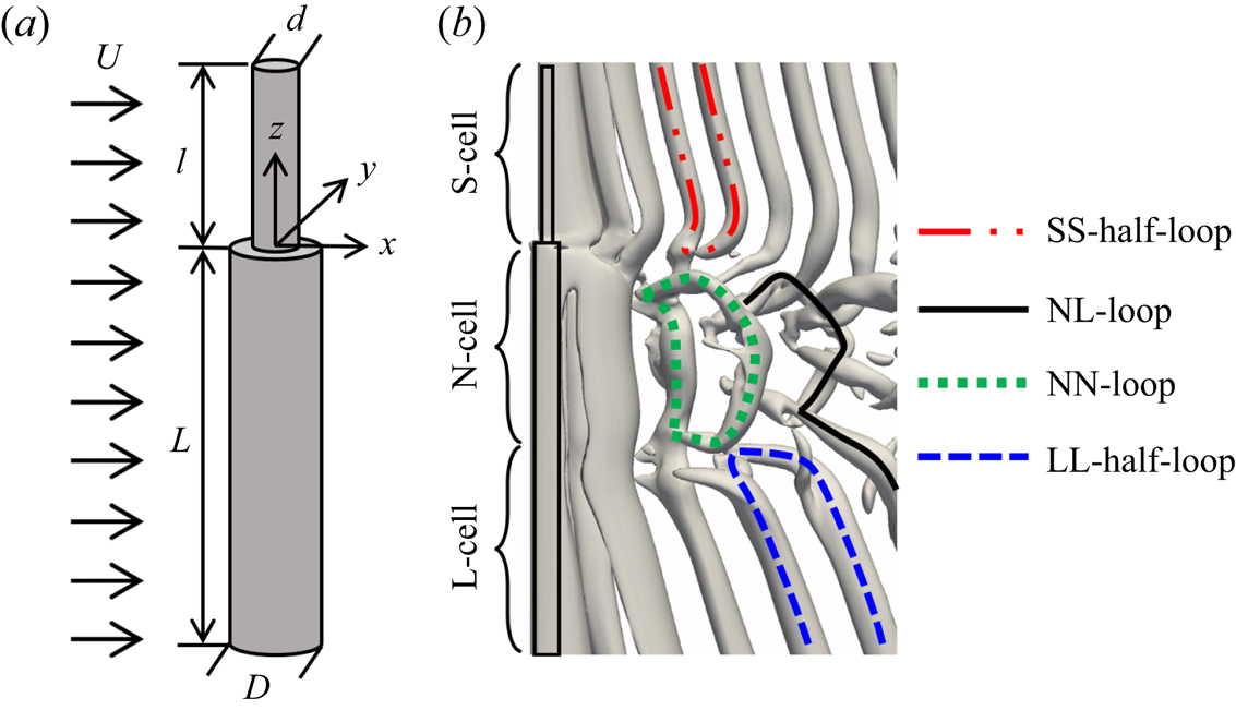
Figure 1. (a) A sketch of the step cylinder geometry. The diameters of the small and large cylinders are  $d$ and
  $D$, respectively. Here,
  $l$ is the length of the small cylinder, and
  $L$ is the length of the large cylinder. The origin is located at the centre of the interface between the small and large cylinders. The uniform incoming flow
  $U$ is in the positive
  $x$-direction. The three directions are named streamwise (
 $x$-direction), cross-flow (
 $y$-direction) and spanwise (
 $z$-direction). (b) Instantaneous wake behind a step cylinder with
  $D/d=2$ at
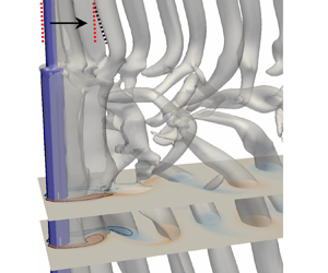
  $Re_D=150$, taken at the moment when vortex dislocations occur. The wake structures are shown by the isosurfaces of
  $\lambda _2=-0.1$ (Jeong & Hussain Reference Jeong and Hussain1995) from the present simulation. The vortex structures (the SS-half-loop, NL-loop, NN-loop and LL-half-loop) that form when the vortex dislocation occurs between the neighbouring vortex cells (the S- and N-cell vortices; the N- and L-cell vortices) are denoted by the coloured curves on the isosurface.
In 1992, Lewis & Gharib (Reference Lewis and Gharib1992) investigated the flow over step cylinders by conducting experiments for  $1.14< D/d<1.76$ at
  $67< Re_D<200$. They mainly discussed two vortex interaction modes: a direct mode for
  $D/d<1.25$ and an indirect mode for
  $D/d>1.55$. For the direct mode, the vortices behind the small and large cylinders exhibit two dominating shedding frequencies
  $f_S$ (small cylinder) and
  $f_L$ (large cylinder), with a direct interaction between them. In the indirect mode, one more frequency
  $f_3$ (also referred to as
  $f_N$ in Dunn & Tavoularis Reference Dunn and Tavoularis2006) was observed between the flow regions dominated by the shedding frequencies
  $f_S$ and
  $f_L$. No direct interaction was observed between vortices with frequencies
  $f_S$ and
  $f_L$. Most of the following research has focused on the indirect mode. Based on an experimental investigation of the wake behind a step cylinder with
  $D/d \approx 2$ at
  $63< Re_D<1100$, Dunn & Tavoularis (Reference Dunn and Tavoularis2006) identified three spanwise (i.e. parallel to the central axis of the cylinder) vortex cells for the indirect mode: (i) the S-cell vortex behind the small cylinder with the highest shedding frequency
  $f_S$, (ii) the L-cell vortex shed from the large cylinder with the shedding frequency
  $f_L$ and (iii) the N-cell vortex located between the S- and L-cell regions shed at the lowest frequency
  $f_N$. Figure 1(b) shows these three vortex cells. The characteristics of these three vortex cells were thereafter investigated by Morton & Yarusevych (Reference Morton and Yarusevych2010, Reference Morton and Yarusevych2020) and Tian et al. (Reference Tian, Jiang, Pettersen and Andersson2017, Reference Tian, Jiang, Pettersen and Andersson2020b, Reference Tian, Jiang, Pettersen and Andersson2021), where most of the vortex interactions are closely related to vortex dislocations. The detailed descriptions are as follows.
The phrase ‘vortex dislocation’ was first introduced by Williamson (Reference Williamson1989) to describe the phenomenon, the contorted ‘tangle’ of vortices, observed in an experiment of the wake behind a circular cylinder with two end plates. Williamson (Reference Williamson1989) found that the vortex dislocation periodically forms when neighbouring vortices move out of phase due to their different shedding frequencies. In the indirect mode of a step cylinder wake, vortex dislocations occur at the boundary between the S- and N-cell vortices and at the boundary between the N- and L-cell vortices. Lewis & Gharib (Reference Lewis and Gharib1992) found that the vortex dislocation between the S- and N-cell vortices occurs within a narrow region, which is time invariant and slightly deflects spanwise into the large cylinder region just behind the step. During the S-N vortex dislocations, it was argued by Lewis & Gharib (Reference Lewis and Gharib1992), Dunn & Tavoularis (Reference Dunn and Tavoularis2006), Morton & Yarusevych (Reference Morton and Yarusevych2010) and McClure, Morton & Yarusevych (Reference McClure, Morton and Yarusevych2015) that the S-cell vortex, except for connecting to the N-cell vortices, connects to the subsequent S-cell vortex shed from the opposite side of the small cylinder and forms SS-half-loop vortices (the red curves in figure 1b). The interactions between the N- and L-cell vortices, however, occur in a relatively wide region (the N–L cell boundary) which varies periodically. Based on the numerical investigations on the flow around a step cylinder with  $D/d=2$ at
  $Re_D=150$ and 300, Morton, Yarusevych & Carvajal-Mariscal (Reference Morton, Yarusevych and Carvajal-Mariscal2009) observed that the shape and spanwise length of the N-cell vortices, as well as the position of the N–L cell boundary, change periodically at the frequency,
  $f_L - f_N$, in accordance with the occurrence of vortex dislocations between the N- and L-cell vortices. They referred to this cyclic variation as the ‘N-cell cycle’. Tian et al. (Reference Tian, Jiang, Pettersen and Andersson2020b) further investigated the vortex dislocation and accumulation of phase differences between the N- and L-cell vortices within the N-cell cycles, by conducting numerical simulations of the flow past a step cylinder with
  $D/d=2$ at
  $Re_D=150$. They identified NN-loop and NL-loop structures in N-cell cycles, as shown by the green dotted and black curves in figure 1(b). The phrases ‘antisymmetric vortex interaction’ and ‘symmetric vortex interaction’ were introduced to describe the phenomenon that the NL-loop structures form on different sides and at the same side of the step cylinder in the neighbouring N-cell cycles, respectively. Moreover, by monitoring the phase information (
 $\varPhi$) of each N- and L-cell vortex over time, Tian et al. (Reference Tian, Jiang, Pettersen and Andersson2020b) described the phase difference accumulation mechanism behind the vortex dislocation process as
 \begin{equation} \varPhi = \varPhi_f + \varPhi_c, \end{equation}
where  $\varPhi$,
  $\varPhi _f$ and
  $\varPhi _c$ represent the total phase difference, the phase difference caused by different vortex shedding frequencies and the phase difference induced by different convective vortex velocities, respectively. This equation implies that the different shedding frequencies and vortex convection velocities are the two qualitatively different physical mechanisms contributing to the accumulation of the phase difference between two neighbouring vortices. The phrases ‘trigger value’ and ‘threshold value’ were applied to describe the values of
  $\varPhi$ and
  $\varPhi _f$ required for the inception of vortex dislocations. These results were further confirmed in a subsequent investigation (Tian et al. Reference Tian, Jiang, Pettersen and Andersson2020a) where the effect of the diameter ratio on the vortex dislocation was investigated numerically in the wake of step cylinders with
  $D/d=2.0$, 2.2, 2.4, 2.6, 2.8 and 3.0 at
  $Re_D=150$. The authors found that as the threshold value of vortex dislocation decreases when
  $D/d$ increases from 2 to 3, the number of dislocated NL vortex pairs and the correspondingly formed NL-loop structures in one N-cell cycle increases from 2 to 4. Although the step cylinder wakes gradually become more complex when
  $Re_D$ increases, the three main spanwise vortices (S-, N- and L-cell vortices) and the vortex dislocation between them were observed at
  $Re_D=300$ (Morton et al. Reference Morton, Yarusevych and Carvajal-Mariscal2009) and at
  $Re_D=1050$ (Morton & Yarusevych Reference Morton and Yarusevych2014). In an experimental investigation of flow around a step cylinder with
  $D/d=2$ at
  $Re_D=1050$, Morton & Yarusevych (Reference Morton and Yarusevych2014) found that the varying duration of the N-cell cycle in the turbulent wake fits a Gaussian distribution. The characteristics of the streamwise vortices around the step were investigated by Dunn & Tavoularis (Reference Dunn and Tavoularis2006), Morton et al. (Reference Morton, Yarusevych and Carvajal-Mariscal2009), Tian et al. (Reference Tian, Jiang, Pettersen and Andersson2021) and Massaro, Peplinski & Schlatter (Reference Massaro, Peplinski and Schlatter2022), where horseshoe-like junction vortices and tip vortices were identified.
Based on an experimental investigation of flow around a step cylinder with  $D/d=2$ at
  $Re_D=80\,000$ (Ko & Chan Reference Ko and Chan1984) and a numerical investigation of flow past a step cylinder with
  $D/d=2$ at
  $Re_D=2000$ (Morton et al. Reference Morton, Yarusevych and Carvajal-Mariscal2009), it was found that the drag force coefficient gradually increases along the large cylinder while decreasing along the small cylinder as the step is approached. However, a detailed description and a physical explanation of the spanwise variation of the structural loads on step cylinders is still lacking.
Previous studies on the single step cylinder have focused on the wake flow development and vortex interactions, but whether and how the wake dynamics affects the structural load along the step cylinder has not yet been thoroughly investigated. The primary goal of the present numerical study is to investigate how the vortex dynamics, especially vortex dislocations, affects the structural load on the step cylinder in detail. To achieve this, we analyse the results obtained from direct numerical simulations (DNS) of the flow past three different step cylinders with diameter ratios  $D/d=2.0$, 2.4 and 2.8 at
  $Re_D=150$. The largest diameter ratio is limited to 2.8 because we want to ensure the appearance of the Kármán vortex street behind the small cylinder. A larger diameter ratio would cause the Reynolds number for the small cylinder to be lower than 50, which is too close to the
  $Re$ range of the closed wake regime (
 $4 \lessapprox Re \lessapprox 48$). To avoid interference of three-dimensional wake instabilities, such as natural vortex dislocation, the Reynolds number for the large cylinder (
 $Re_D$) is set to 150, which is lower than
  $Re \approx 180$ where the uniform cylinder wake starts becoming three-dimensional.
The paper is organized as follows: in § 2, the flow problem and the numerical settings are addressed. Section 3 first revisits the three main vortex cells in the wake, i.e. the S-, N- and L-cell vortices. Then, the non-parallel shedding of the S- and L-cell vortices are discussed in all three cases, where the mechanism behind the non-parallel shedding of the S-cell vortices is provided. In § 4, based on the  $D/d=2.0$ case, the effects of the wake flow on the structural load over the step cylinder, especially the effects of vortex dislocations on structural loads, are analysed. In § 5, we discuss the robustness of discussions and conclusions in § 4 as well as the diameter ratio effects on the structural loads by investigating the
  $D/d=2.4$ and 2.8 cases.
2. Governing equations, boundary conditions and convergence study
The incoming flow  $U$ is uniform in the positive
  $x$-direction. The diameter ratio of the step cylinder is given as 2.0, 2.4 and 2.8. The Reynolds number is
  $Re_D=150$, based on the diameter of the large cylinder. The origin of the coordinate system is at the step as shown in figures 1 and 3. The incompressible flow is governed by the continuity equation and the time-dependent three-dimensional incompressible Navier–Stokes equation
 \begin{gather} \boldsymbol{\nabla} \boldsymbol{\cdot} \boldsymbol{u}=0, \end{gather}
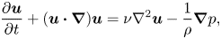 \begin{gather} \frac{\partial \boldsymbol{u}}{\partial t} + (\boldsymbol{u} \boldsymbol{\cdot} \boldsymbol{\nabla})\boldsymbol{u} = \nu {\nabla}^{2} \boldsymbol{u} - \frac{1}{\rho} \boldsymbol{\nabla} p, \end{gather}
where  $\rho$ is the constant fluid density, while
  $\boldsymbol {u}$,
  $p$ and
  $t$ denote the velocity vector, pressure and time, respectively.
Direct numerical simulations were conducted by using a finite-volume numerical code MGLET (Manhart Reference Manhart2004). This code has been thoroughly validated in previous works for various applications, for example, the flow around step cylinders (Tian et al. Reference Tian, Jiang, Pettersen and Andersson2020b, Reference Tian, Jiang, Pettersen and Andersson2021), the flow around a prolate spheroid (Jiang et al. Reference Jiang, Pettersen, Andersson, Kim and Kim2018), the flow around a cylinder–wall junction (Schanderl et al. Reference Schanderl, Jenssen, Strobl and Manhart2017) and the oscillatory flow through a hexagonal sphere pack (Unglehrt & Manhart Reference Unglehrt and Manhart2022). The numerical grid is staggered such that the velocities are located in the middle of the grid face, and the pressure is evaluated in the middle of the grid cell. The midpoint rule is used to approximate the surface integral, leading to second-order accuracy. A third-order Runge–Kutta scheme (Williamson Reference Williamson1980) is applied for the time integration. A constant time step  $\Delta t$ is used to ensure a CFL (Courant–Friedrichs–Lewy) number smaller than 0.5. Stone's implicit procedure (Stone Reference Stone1968) is applied to solve the elliptic pressure correction equation. The step cylinder geometry is handled by an immersed boundary method (Peller et al. Reference Peller, Duc, Tremblay and Manhart2006; Peller Reference Peller2010).
By implementing the zonally embedded grid method (Manhart Reference Manhart2004), the computational domain is first equally divided into cubic grid boxes, called the level-1 box. There are  $N \times N \times N$ equally sized cubic grid cells in each grid box. The local grid refinement in the region where complex flow phenomena occur (e.g. the regions close to the step cylinder and the region where vortices form) is achieved by continuously dividing the grid box (the level-1 box) into eight smaller grid boxes, denoted the level-2 box. In each level-2 box, there are also
  $N \times N \times N$ equally sized cubic grid cells. This grid-refinement process continues until the finest specified grid level is reached (all simulations in this study have six grid levels). Figure 2 schematically illustrates the grid structure in the symmetry plane (the
  $xz$-plane at
  $y/D=0$) in the Fine-28A case shown in the third row of table 1.
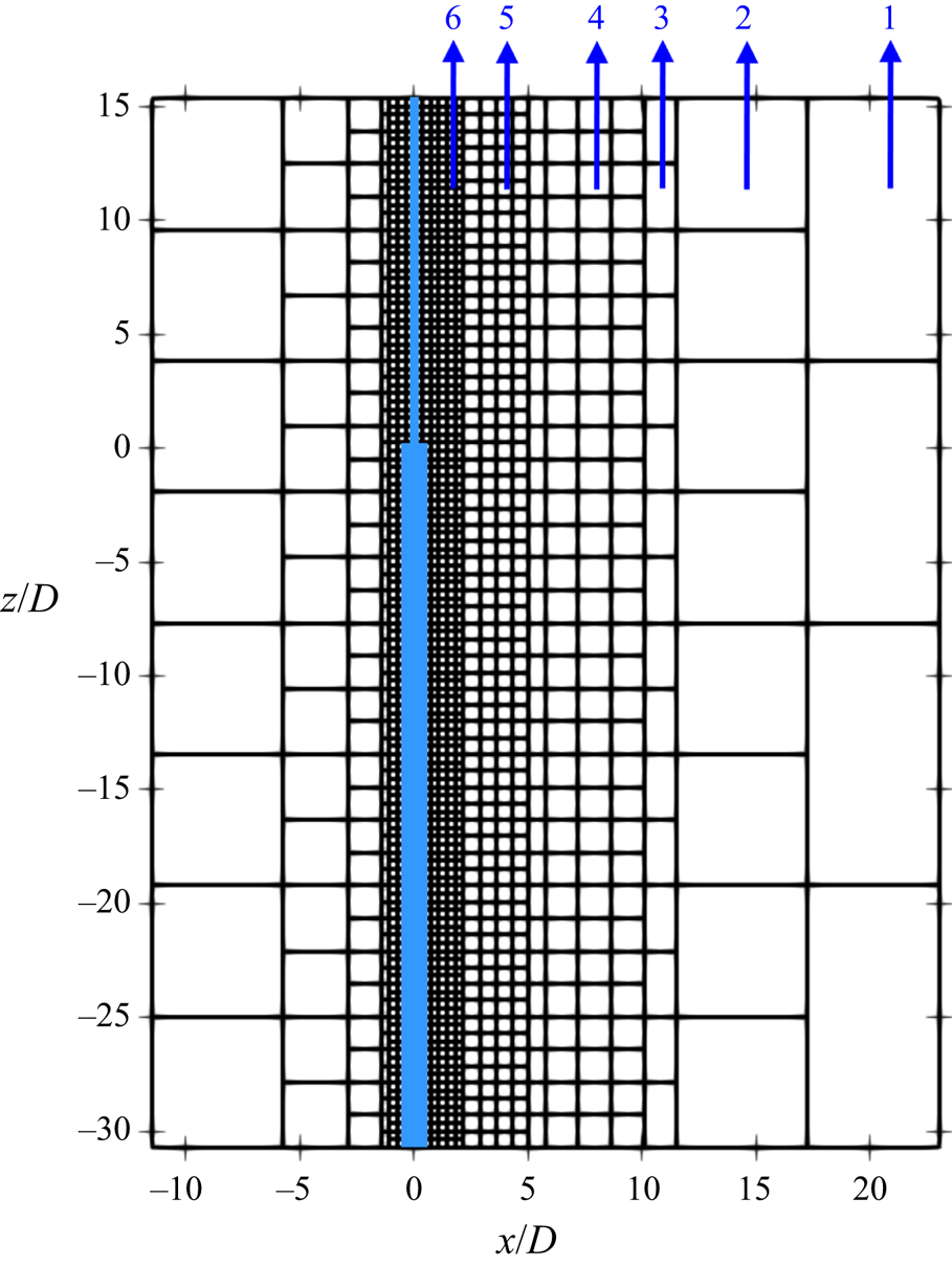
Figure 2. An illustration of the multi-level grids in the  $xz$-plane at
  $y/D=0$. Each square represents a slice of the corresponding cubic Cartesian grid box that contains
  $N \times N \times N$ grid cells. Here, there are six levels of grid boxes as indicated by numbers.
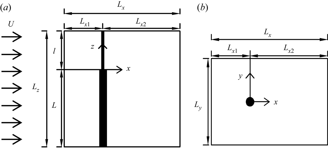
Figure 3. Computational domain and coordinate system are illustrated from (a) side view and (b) top-down view.
Table 1. Mesh and computational domain information of all simulations in the present study. The case Coarse has five levels of grids, and the other cases all have six levels of grids. The cases Coarse, Medium and Fine-28A are used for the grid study. The cases Fine-28A, Fine-28B and Fine-28C are used for the spanwise length study. As shown in figure 2, the minimum grid cells ( $\varDelta _c/D$) cover the region around the step cylinder.
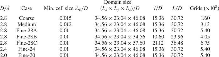
Figure 3 shows the side and top-down views of the flow domain. The streamwise length of the flow domain is  $L_x$, where
  $L_{x1}$ and
  $L_{x2}$ are the distance from the inlet and outlet planes to the centre of the step cylinder, respectively. In the cross-flow direction, the length of the flow domain is
  $L_y$, where the step cylinder is located in the middle. The spanwise height of the domain is
  $L_z$, where the length of the small and large cylinders is
  $l$ and
  $L$, respectively. A constant velocity profile (
 $u=U$ and
  $v=w=0$) is applied at the inlet. At the outlet, a Neumann condition (
 $\partial u/\partial x =\partial v / \partial x=\partial w / \partial x=0$) is applied. A free-slip boundary condition is applied for the other four sides of the computational domain (for the two vertical sides
  $v=0$,
  $\partial u / \partial y = \partial w / \partial y = 0$; for the two horizontal sides:
  $w=0$,
  $\partial u / \partial z = \partial v / \partial z = 0$). A no-slip condition (
 $u=v=w=0$) is imposed at the step cylinder surface. Neumann conditions are applied for the pressure, except at the outlet where the pressure is set equal to zero.
One grid convergence and one spanwise length convergence study have been conducted and reported in Appendix A. The three cases denoted Coarse, Medium and Fine-28A are selected for the grid convergence study. The computational domain applied in the present study is larger than that used by Morton & Yarusevych (Reference Morton and Yarusevych2010) and Tian et al. (Reference Tian, Jiang, Pettersen and Andersson2020b,Reference Tian, Jiang, Pettersen and Anderssona) for the same step cylinder and  $Re_D$. Therefore, only the spanwise convergence study has been conducted (based on the Fine-28A, Fine-28B and Fine-28C cases) to ensure that the free-slip boundary condition used at the top and bottom boundaries has a minor effect on the discussion and conclusion of this study. Table 1 shows an overview of all the simulations conducted in this work. Based on the convergence study, it is concluded that the configuration and mesh for the Fine-28A case are adequate for reliable DNS simulations in the present study.
3. Vortex formation and flow structures
Figure 4 shows an overview over the vortex structures in the wake behind the  $D/d=2.0$, 2.4 and 2.8 cases, where the extensions of the S-, N- and L-cell vortices are marked. Besides the clear vortex dislocations between the neighbouring vortex cells which have been systematically investigated in previous papers (Dunn & Tavoularis Reference Dunn and Tavoularis2006; Morton et al. Reference Morton, Yarusevych and Carvajal-Mariscal2009; Tian et al. Reference Tian, Jiang, Pettersen and Andersson2017, Reference Tian, Jiang, Pettersen and Andersson2020b), another interesting phenomenon is the non-parallel vortex shedding (relative to the spanwise direction) occurring in the S-cell region as well as in the L-cell region. It should be noted that, away from the NL-cell boundary, the non-parallel shedding in the L-cell region with a constant shedding angle is the conventional oblique shedding (Williamson Reference Williamson1989) and has been discussed previously in Tian et al. (Reference Tian, Jiang, Pettersen and Andersson2017). But the non-parallel shedding in the S-cell region is an uncommon non-uniform oblique shedding, with a shedding angle varying in the spanwise direction. This phenomenon has not been thoroughly explained before and will be further discussed below.
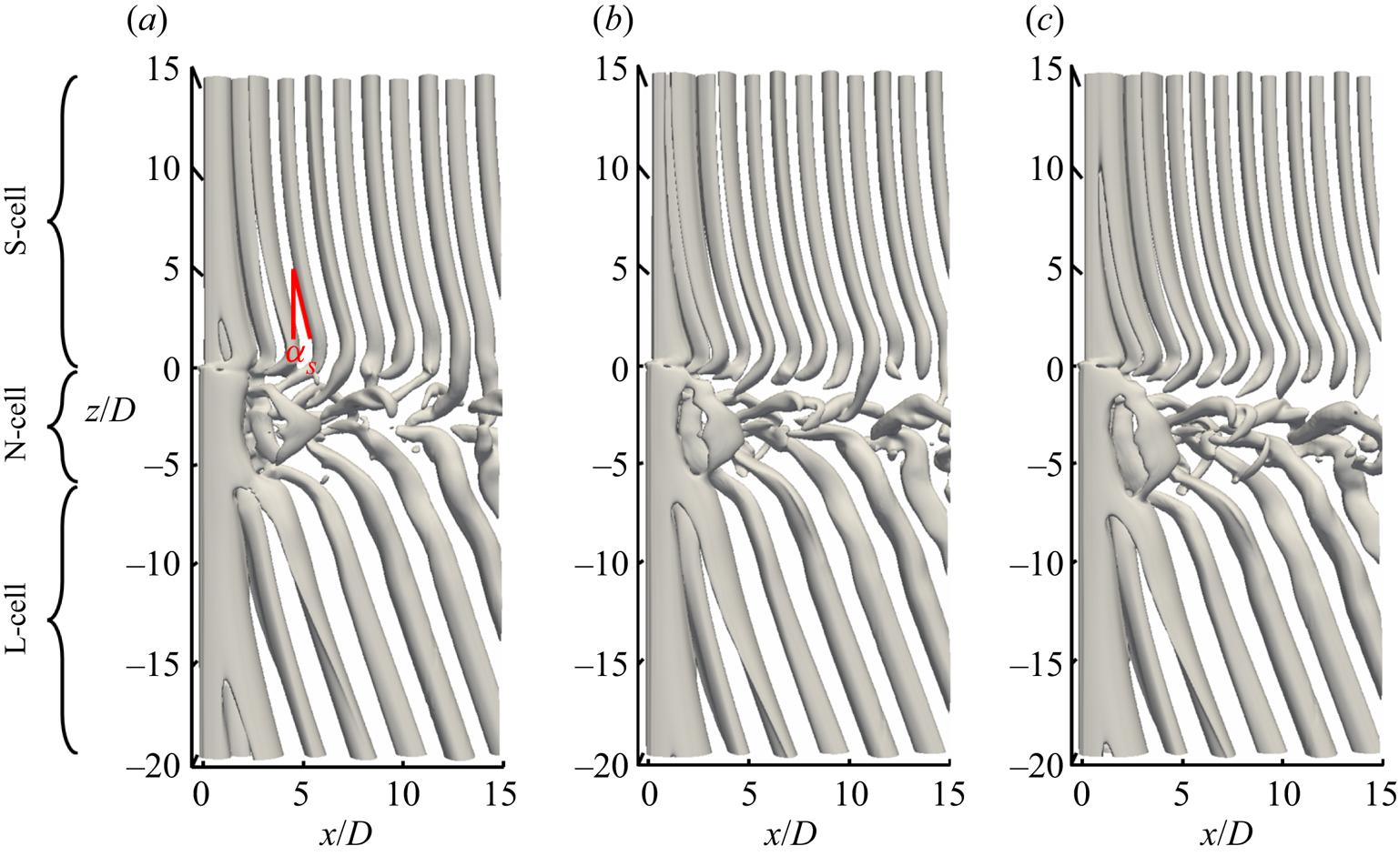
Figure 4. Instantaneous isosurface of  $\lambda _2=-0.05$ at
  $Re_D=150$: (a) the
  $D/d=2.0$ case, (b) the
  $D/d=2.4$ case and (c) the
  $D/d=2.8$ case. The approximate extensions of the three vortex cells (S-, N- and L-cell vortices) and the local shedding angle
  $\alpha _L$ of the L-cell vortices and
  $\alpha _S$ of the S-cell vortices are indicated.
The local angle of the S-cell vortex tubes relative to the cylinder axis,  $\alpha _S$, is shown in figure 4(a). Since
  $\alpha _S$ varies from one shedding cycle to another in the vicinity of the SN-cell boundary, as shown in figure 4(a), we measure the spanwise distribution of
  $\alpha _S$ by tracking and averaging the angle of ten fully developed S-cell vortices for
  $z/D>2.5$. The result is shown in figure 5(a). It appears that
  $\alpha _S$ drastically increases in the vicinity of the step (
 $z/D=0$), and the increase rate is larger for the larger
  $D/d$ case. Table 2 shows the Strouhal number of the S-cell vortex
  $St_S$ from the present simulations and the corresponding empirical Strouhal number
  $St'_S$ from Norberg (Reference Norberg2003). There is a good agreement between
  $St_S$ and
  $St'_S$ without application of the well-known recasting relation of the oblique shedding proposed by Williamson (Reference Williamson1989):
  $St = St_{\alpha }/\cos (\alpha ),$ where
  $\alpha$ is the oblique shedding angle;
  $St_\alpha$ and
  $St$ represent the oblique shedding and the parallel shedding frequencies, respectively. The largest discrepancy is around 2 %, indicating that the non-uniform oblique shedding of the S-cell vortex is different from the conventional oblique shedding (Williamson Reference Williamson1989). By experimental investigations of the flow around a step cylinder with
  $D/d \approx 2.0$ at
  $62< Re_D<110$, Dunn & Tavoularis (Reference Dunn and Tavoularis2006) observed this S-cell shedding phenomenon: all the S-cell vortices are inclined such that the part of the vortex away from the step is always farther upstream than the part of the vortex closer to the step. Dunn & Tavoularis suggested that the underpinning mechanism might be due to the step-induced spanwise flow triggering the early shedding of the S-cell vortex close to the step surface. After a thorough investigation based on the present numerical study, we confirm their suggestion and further find that the appearance of non-uniform oblique shedding is mainly caused by the simultaneous increase of base suction and vortex formation length in the S-cell region in the vicinity of the step.
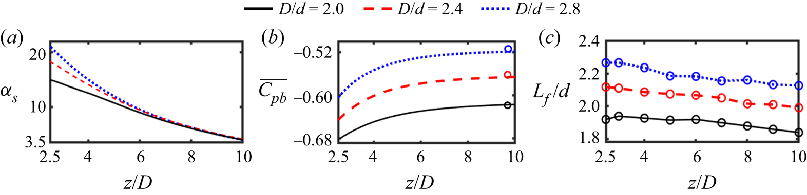
Figure 5. Spanwise distribution of (a) the angle of the vortex tubes in the S-cell region ( $z/D>2.5$); (b) the time-averaged base pressure coefficient
  $\overline {C_{pb}}$ on the small cylinder part; (c) the vortex formation length
  $L_f/d$ on the small cylinder part. In (b), the circle represents the corresponding base pressure obtained from Rajani, Kandasamy & Majumdar (Reference Rajani, Kandasamy and Majumdar2009). Here,
  $\overline {C_{pb}}$ is given by
  $\overline {C_{pb}}=(\overline {P_b}-P_0)/(0.5\rho U^2)$, where
  $P_0$ is the pressure at the outlet boundary and
  $\overline {P_b}$ is the time-averaged pressure along a sampling line 0.02
 $D$ behind the cylinder wall in the
  $xz$-plane at
  $y/D=0$. The distance
  $h=0.02D$ is selected because it is slightly larger than the smallest cell's diagonal (
 $\sqrt {2}\varDelta < h=0.02D<1.5\sqrt {2}\varDelta$ where
  $\varDelta =0.01D$) such that we safely avoid the wiggles possibly caused by cells directly cut by the cylinder surface and still stay as close as possible to the surface.
Table 2. The Strouhal number of the S-cell vortex ( $St_S = f_S D/U$) is obtained from a discrete Fourier transform of the time series of the streamwise velocity
  $u$ along a vertical sampling line positioned at
  $(x/D, y/D)=(0.6, 0.2)$ over at least 1000 time units (
 $D/U$) for three cases. In the third column, the empirical Strouhal number of the small cylinder (
 $St'_S$) is calculated by using equation
  $St'_S=(0.2663-1.019/Re_d^{0.5})\times D/d$ from Norberg (Reference Norberg2003).
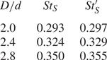
Figure 5(b) shows the time-averaged base pressure coefficient  $\overline {C_{pb}}$ along a spanwise sampling line located
  $0.02D$ downstream of the small cylinder wall at
  $y/D=0$. The corresponding
  $\overline {C_{pb}}$ for a uniform circular cylinder is also given. Figure 5(c) shows the spanwise distribution of the averaged vortex formation length (
 $L_f$), obtained by tracking and averaging the development of ten S-cell vortices (an example will be shown in figure 7 later). It appears that the base suction behind the small cylinder far from the step coincides with those for the corresponding uniform cylinder. As the step is approached, figure 5(c,d) shows that the base suction and the vortex formation length simultaneously increase. It should be noted that a decrease in the base suction is usually accompanied by an increased vortex formation length and a decrease in the vortex shedding frequency, e.g. in the wake behind a free-end cylinder (Ayoub & Karamcheti Reference Ayoub and Karamcheti1982) and in the wake behind a concave curved cylinder (Jiang et al. Reference Jiang, Pettersen, Andersson, Kim and Kim2018). Contrary to the case described above, the simultaneously increased base suction and vortex formation length leads to the part of the S-cell vortex in the vicinity of the step to shed farther downstream than the part of the S-cell vortex farther away from the step in the cylinder axis, with the same shedding frequency. This results in the non-uniform oblique shedding of the S-cell vortex shown in figure 4. The underpinning mechanism will be explained as follows. First, the mixing of wakes behind the small and large cylinders causes the suction pressure and the recirculation length to increase behind the small cylinder. In figure 6, the time-averaged pressure contour and streamlines are plotted in the
  $xz$-plane at
  $y/D=0$ in the
  $D/d=2.0$ and 2.8 cases. The red curve denotes the position where the time-averaged streamwise velocity is zero, indicating the recirculation region. It appears that, far from the step, the small suction pressure region (the yellow region) is closer to the small cylinder than the larger cylinder due to the different diameters. Close to the step, the wakes behind the small and large cylinders are mixed and smoothly connected. Consequently, the suction pressure in the vicinity of the step increases behind the small cylinder and decreases behind the large cylinder as shown in figures 5(b) and 6(a,b). A similar transition process also appears for the recirculation length behind the small and large cylinders. The small and large cylinder wakes are mixed around the step (
 $z/D=0$), causing the recirculation region to move farther away from the small cylinder wall but closer to the large cylinder wall when the step is approached, as shown in figure 6(c,d).

Figure 6. The time-averaged pressure contour in the  $xz$-plane at
  $y/D=0$ (a) in the
  $D/d=2.0$ case, (b) in the
  $D/d=2.8$ case. The time-averaged streamlines in the region marked by the red rectangle in (a) are plotted in (c) in the
  $D/d=2.0$ case, (d) in the
  $D/d=2.8$ case. The location where the recirculation region ends is outlined by the red curve in (c,d); the coordinates of three representative locations are also denoted.
Then, the above-described pressure variation behind the step cylinder induces a downwash flow directed from the small cylinder to the large cylinder, which accelerates the production rate of circulation of the S-cell vortex strength and finally causes non-uniform oblique shedding in the S-cell region. Figure 6(c) shows that the induced downwash flow causes the streamlines pointing to the small cylinder wall to change from horizontal to inclined as the step is approached along the small cylinder. This downwash flow mainly splits into two parts: one joins and accelerates the production rate of the vortex circulation behind the small cylinder, and the other one moves down into the large cylinder wake. To show the acceleration of the circulation production rate, the instantaneous flow characteristics are checked in the small cylinder wake for  $D/d=2$. According to Green & Gerrard (Reference Green and Gerrard1993) and Griffin (Reference Griffin1995), the end of the vortex formation region coincides with the location where the vortex strength becomes maximum. The circulation strength of the S-cell vortex in the present work is defined as the integration of the spanwise vorticity
  $\omega _z$ in the area (A) enclosed by the corresponding isoline
  $\lambda _2=-1.7$ (Jeong & Hussain Reference Jeong and Hussain1995) based on (3.1)
 \begin{equation} \varGamma =\oint {|\omega_z|}\boldsymbol{\cdot} {\rm d}{A}, \end{equation}
The moment when the S-cell vortex just forms can be obtained by tracking the variation of its vortex strength. The time evolution of the vortex strength of two consecutive S-cell vortices in the  $xy$-plane close to the step at
  $z/D=3$ as well as in the
  $xy$-plane far from the step at
  $z/D=10$ are calculated and shown in figures 7(a) and 7(c), respectively. The time of occurrence and vortex strength for the peak values
  $P1$,
$P1$,  $P2$,
$P2$,  $P3$ and
  $P4$ are also given. Figure 7(b,d) shows the contour of instantaneous spanwise vorticity (
 $\omega _z$) at the peaks
  $P1$ and
  $P3$ in figure 7(a,c). By detecting the centre of the region surrounded by the white (
 $\lambda _2=-1.7$) and black (
 $\lambda _2=-3$) iso-lines, the formation position of the monitored S-cell vortex is marked by the green line. The time duration between the peaks
  $P1$ and
  $P2$ in figure 7(a) and
  $P3$ and
  $P4$ in figure 7(c) are the same, indicating that the time duration between two consecutive S-cell vortices is the same whether the monitoring plane is close to the step or not. It can be seen that the S-cell vortex in the
  $xy$-plane at
  $z/D=3$ is stronger and is located farther downstream compared with the S-cell vortex in the
  $xy$-plane at
  $z/D=10$ when these vortices just form. This means that, as the step is approached from the small cylinder, the induced spanwise flow increases the production rate of the vortex strength, which makes the S-cell in this region able to keep the shedding frequency unchanged but it forms farther downstream. A similar process also appears in the
  $D/d=2.4$ and 2.8 cases. Moreover, the increased diameter ratio strengthens the increase of the base suction and the vortex formation length as shown in figure 5(b,c), leading to a large increase rate of the oblique shedding angle as the step is approached along the small cylinder, as shown in figure 5(a).
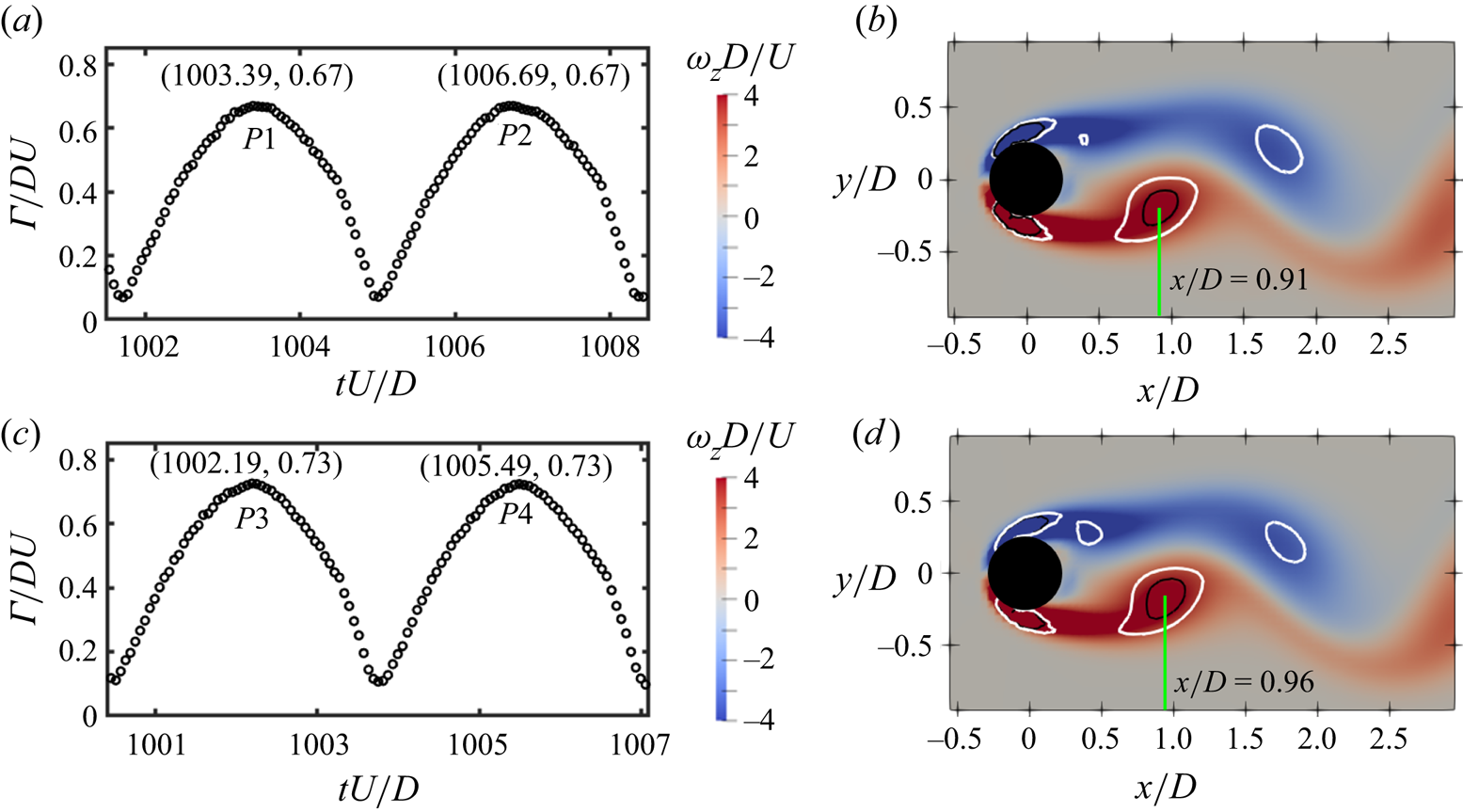
Figure 7. (a) Time evolution of the vortex strength  $\varGamma /DU$ of two consecutive S-cell vortices in the
  $xy$-plane at
  $z/D=10$. The vortex strength is integrated within the white isoline
  $\lambda _2=-1.7$. (b) The instantaneous spanwise vorticity
  $\omega _z$ in the
  $xy$-plane at
  $z/D=10$ at
  $tU/D=1003.45$ (the peak
  $P1$ in panel a). (c) Same as panel (a) but in the
  $xy$-plane at
  $z/D=3$. (d) Same as panel (b) but in the
  $xy$-plane at
  $z/D=3$ at
  $tU/D=1001.71$ (the peak
  $P3$ in panel c). The time of occurrence and vortex strength for four peaks (
 $P1$,
$P1$,  $P2$,
$P2$,  $P3$ and
  $P4$) are marked in (a,c). The formation position of the monitored S-cell vortex is obtained by detecting the centre of the white (
 $\lambda _2=-1.7$) and black (
 $\lambda _2=-3.0$) isolines.
In general, the simultaneous increase of the base suction and the vortex formation length in the S-cell region as the step is approached cause an increase of the production rate of vortex strength, moving the vortex formation position farther downstream. Consequently, the non-uniform oblique shedding of the S-cell vortex appears.
4. Structural loads on the step cylinder with  $D/d=2$

The present section is divided into three parts. In the first part, the mechanism underpinning the effect of the vortex dislocations on the structural load is discussed. In the last two parts, the structural load on the small and large cylinders is discussed. All discussions in the present section are based on the  $D/d=2.0$ case.
In the following context, the definitions of the time-averaged drag coefficient  $\overline {C_D}$ and the root-mean-square of the lift coefficient
  $\overline {C'_L}$ are
 \begin{gather} \overline{C_D} = \frac{1}{N}\sum_{i=1}^{N}\frac{2 F_{D,i}(t)}{\rho U^2 D_p L_c}, \end{gather}
 \begin{gather} \overline{C'_L} = \sqrt{ \frac{2}{N}\sum_{i=1}^{N}(C_{L,i}-\overline{C_L})^2}, \end{gather}
 \begin{gather} C_L = \frac{2 F_L(t)}{\rho U^2 D_p L_c}, \end{gather}
 \begin{gather} \overline{C_L} = \frac{1}{N}\sum_{i=1}^{N} C_{L,i}, \end{gather}
where  $N$ is the number of values in the sample,
  $F_D(t)$ and
  $F_L(t)$ are the sampled drag and lift forces acting on the structure, respectively. Here,
  $D_p=D$ for the large cylinder and
  $D_p=d$ for the small cylinder;
  $L_c$ is the spanwise length of the part of the step cylinder where the forces are sampled (
 $L_c$ is set as 0.2
 $D$ for the simulation with
  $\varDelta _{min}=0.01$). The laminar vortex shedding in the wake causes the structural load of the step cylinder to be primarily induced by the pressure on the cylinder wall. Therefore, when the variation of the structural load is discussed in the forthcoming section, the focus will be on the vortex interactions in the near wake.
4.1. Vortex dislocation effects on structural load
As a fundamental physical phenomenon, the effect of vortex dislocation on the structural load has been reported for various flows, e.g. the flow around a circular cylinder (Qu et al. Reference Qu, Norberg, Davidson and Peng2013; Behara & Mittal Reference Behara and Mittal2020) and the flow around a circular cylinder with a downstream sphere (Zhao Reference Zhao2021). In these studies, the authors observed that both the drag and lift decrease at the position where the vortex dislocation occurs. Zhao (Reference Zhao2021) explained this as a consequence of the spanwise vortices being weakened by the corresponding vortex dislocations. However, this mechanism does not fully explain the complex force variations over the step cylinder during vortex dislocations. A more detailed discussion about the effect of vortex dislocation on the structure load is given as follows.
The contour of cross-flow velocity  $v$ is plotted along a spanwise sampling line at
  $(x/D, y/D)=(0.6, 0)$ in figure 8(a), where the contours of positive and negative values are induced by the vortex shed from the
  ${+}Y$ and
  ${-}Y$ sides of the step cylinder, respectively. From
  $tU/D=670$ to 730, the one-to-one relationship between N- and L-cell vortices gradually breaks up, i.e. a vortex dislocation occurs, as marked by the black thick line in figure 8(a); the mean dislocation position (illustrated by the red line at
  $z/D=-5.5$ in figure 8a) is defined as the centre of the black line. For the same time window, figure 8(b,c) shows the time history of
  $C_D$ and
  $C_L$ at the mean dislocation position. From the blue line to the green line (where vortex dislocation occurs) in figure 8(b,c), the fluctuation amplitude of
  $C_D$ decreases 5.7 % (from 1.278 to 1.207), while the fluctuation amplitude of
  $C_L$ almost decreases 90 % (from 0.456 to 0.05). The distinct rates of decrease of
  $C_D$ and
  $C_L$ during this time interval are caused by a combined effect of the decreased spanwise vortex strength and the temporarily weakened staggered Kármán vortex shedding during the dislocation process.

Figure 8. (a) Cross-flow velocity component  $v$ as a function of the non-dimensional time, along the spanwise sampling line at
  $(x/D, y/D)=(0.6, 0)$ in the
  $D/d=2.0$ case. The black line sketches the position where vortex dislocations occur between the N- and L-cell vortices. The averaged dislocation position is defined as the centre of the black line and illustrated by the red line. (b,c) Time history of
  $C_D$ and
  $C_L$ at
  $z/D=-5.5$ (the horizontal red line in panel a) in the
  $D/d=2.0$ case.
Figures 9(a–e) and 10(a–e) show the shedding process of the N- and L-cell vortices without and with vortex dislocations, respectively. The N- and L-cell vortices are labelled by a combination of capital letters and numbers: ‘N’ and ‘L’ represent N- and L-cell vortices, respectively, while the number indicates the shedding order. The primes are used to denote the vortices shed from the  ${+}Y$ side. The red solid line sketches the boundary between the N- and L-cell vortices. Figures 9(f–j) and 10(f–j) show the corresponding contours of vorticity
  $\omega _z$ in the
  $xy$-plane at the mean dislocation position (
 $z/D=-5.5$). Figures 9(k) and 10(k) show the time variation of
  $C_L$ over one period. The one-to-one relation between N- and L-cell vortices (e.g. N’1–L’1, N2–L2) is clearly shown in figure 9(a–e). After seven N–L vortex pairs, the accumulated phase difference (Tian et al. Reference Tian, Jiang, Pettersen and Andersson2020b) caused by the different shedding frequencies,
  $f_N$ and
  $f_L$, makes L8 dislocate from its counterpart N8 on the
  ${-}Y$ side and connect to N’7 located on the
  ${+}Y$ side, as shown in figure 10(a–d). Further details of vortex dislocation processes can be found in Tian et al. (Reference Tian, Jiang, Pettersen and Andersson2017, Reference Tian, Jiang, Pettersen and Andersson2020b). The decreased spanwise coherence of the N- and L-cell vortices together with the formation of the cross-border connection between the N- and L-cell vortices (e.g. N’7–L8 in figure 10d) during the vortex dislocation process severely suppressed the staggered Kármán vortex shedding, as shown in figure 10(g–j), compared with the vortex shedding shown in figure 9(f–j) during a time interval without vortex dislocation. In figure 10(g–j), the spanwise vorticity
  $\omega _z$ is distributed much more symmetrically between the
  ${+}Y$ and
  ${-}Y$ sides than that during the interval without vortex dislocation, as shown in figure 9(g–j). This is further visualized in figure 11(a,b), showing close ups of figure 9(g) and figure 10(g), adding black isolines of
  $\omega _z = \pm 3$ to visualize the shape of the strong spanwise vorticity regions. Moreover, the magnitude of the circulation in the near wake of the cylinder is calculated within the black solid and dotted rectangles, as shown in figure 11(a,b). Figure 11(c) shows the circumferential distribution of the pressure on the section of the step cylinder shown in figure 11(a,b). The amount of circulation within the near wake region (marked by the black sold and dashed rectangles in figure 11) slightly decreases from 2.9 (
 $1.7+1.2=2.9$) at
  $t2$ in figure 11(a) to 2.7 (
 $1.4+1.3=2.7$) at
  $t7$ in figure 11(b). However, the circulation difference between the black solid rectangle (behind the upper side of the cylinder) and the black dotted rectangle (behind the lower side of the cylinder) sharply decreases from 0.5 (
 $1.7-1.2=0.5$) to 0.1 (
 $1.4-1.3=0.1$). As a result, when vortex dislocation occurs from t2 to t7, the difference between the circumferential pressure along the
  ${+}Y$ and
  ${-}Y$ sides of the cylinder decreases, as shown in figure 11(c). The slightly decreased total circulation and the base suction induce a small reduction in
  $C_D$, while the less asymmetric circulation and base suction between the
  ${+}Y$ and
  $-Y$ sides of the large cylinder wake cause a large reduction in
  $C_L$, as shown in figure 8(c).

Figure 9. Isosurface of  $\lambda _2=-0.05$ showing shedding of N- and L-cell vortices when there is no vortex dislocation in the
  $D/d=2.0$ case: (a)
  $tU/D=t1$, (b)
  $tU/D=t2$, (c)
  $tU/D=t3$, (d)
  $tU/D=t4$, (e)
  $tU/D=t5$. (f–j) The corresponding instantaneous vorticity
  $\omega _z$ contour in the
  $xy$-plane at
  $z/D=-5.5$ (the red line marked in panels a–e). (k) Time history of the lift force coefficient
  $C_L$. Five typical time instants
  $t1$–
$t1$– $t5$ are marked.

Figure 10. Isosurface of  $\lambda _2=-0.05$ showing shedding of N- and L-cell vortices when vortex dislocations occur in the
  $D/d=2.0$ case: (a)
  $tU/D=t6$, (b)
  $tU/D=t7$, (c)
  $tU/D=t8$, (d)
  $tU/D=t9$, (e)
  $tU/D=t10$. (f–j) The corresponding instantaneous vorticity
  $\omega _z$ contour in the
  $xy$-plane at
  $z/D=-5.5$ (the red line marked in panels a–e). (k) Time history of the lift force coefficient
  $C_L$. Five typical time instants
  $t$6–
$t$6– $t$10 are marked.

Figure 11. Contour of instantaneous vorticity  $\omega _z$ in the
  $xy$-plane at
  $z/D=-5.5$: (a) at
  $t2$ shown in figure 9(g); (b) at
  $t7$ shown in figure 10(g); (c) the circumferential distribution of instantaneous pressure along the cylinder slices in (a,b). The position angle
  $\theta$ is measured from the front stagnation point, i.e.
  $\theta =180$ represents the rear stagnation point. The shape of the concentrated
  $\omega _z$ region is shown by the black isoline of
  $\omega _z$ =
  $\pm$ 2. Based on (3.1), the circulation in the region marked by the black and dotted rectangles in (a,b) is calculated and shown.
The vortex dislocation process described above agrees well with the findings in previous publications (Morton et al. Reference Morton, Yarusevych and Carvajal-Mariscal2009; Tian et al. Reference Tian, Jiang, Pettersen and Andersson2020b); the detailed investigations reveal that, although the vortex dislocation between the N- and L-cell vortices form somewhat away from the step cylinder (consistent with Tian et al. Reference Tian, Jiang, Pettersen and Andersson2020b), the vortex dislocation drastically affects the sectional drag and lift. Overall, during the vortex dislocation process, a larger rate of decrease for  $C_L$ than for
  $C_D$ is caused by a combined effect of the decreased circulation and the weakened staggered Kármán vortex shedding, where the latter plays the major role.
4.2. Drag force characteristics
Figure 12(a) shows the time-averaged drag coefficient  $\overline {C_D}$ along the step cylinder. The contributions from the pressure (
 $\overline {C_{Dp}}$) and skin friction (
 $\overline {C_{Df}}$) on
  $\overline {C_D}$ shown in figure 12(b) indicate that the variation of
  $\overline {C_D}$ is attributed primarily to the pressure.

Figure 12. In the  $D/d=2.0$ case: (a) the spanwise distribution of the total drag coefficient (
 $\overline {C_D}$); (b) the spanwise distribution of the viscous (
 $\overline {C_{Df}}$) and pressure (
 $\overline {C_{Dp}}$) drag coefficients. In (a), two local extremes of the total drag coefficient (
 $EX_{DS}$ and
  $EX_{DL}$) are denoted. Several noteworthy variations of
  $\overline {C_D}$ are sketched.
Along the small cylinder, it appears that  $\overline {C_D}$ increases from
  $z/D=15$ to the local maximum point
  $EX_{DS}$ (
 $z/D=0.78$), and then decreases sharply towards the step. The increase of
  $\overline {C_D}$ as the step is approached is caused by the strengthened suction pressure in the vicinity of step behind the small cylinder, as shown in figure 6(a) and discussed in § 3. This is further visualized by the time-averaged circumferential pressure distributions on the small cylinder at
  $z/D=0.8$ (red), and
  $z/D=10$ (black) in figure 13(c). The sharply decreased
  $\overline {C_D}$ from
  $EX_{DS}$ towards the step is caused by a combined effect of the decreased stagnation pressure at
  $\theta =0$ and the weakened suction pressure from
  $\theta =70$ to
  $\theta =180$, as shown by the red and green curves in figure 13(c). The decreased stagnation pressure is induced by the formation of the junction vortex visualized by the time-averaged streamlines and pressure contour in the
  $xz$-plane at
  $y/D=0$ in figure 13(a,b), respectively. Similar to the findings by Morton et al. (Reference Morton, Yarusevych and Carvajal-Mariscal2009), McClure et al. (Reference McClure, Morton and Yarusevych2015), Tian et al. (Reference Tian, Jiang, Pettersen and Andersson2021) and Massaro et al. (Reference Massaro, Peplinski and Schlatter2022), a junction vortex is located near the step region in figure 13(a). The corresponding low-pressure zone (highlighted by the black rectangle in figure 13b) causes the stagnation pressure on the small cylinder wall (marked by the black dotted rectangle) to become lower than that observed farther away from the step. The weakened suction pressure in the vicinity of the step behind the small cylinder is mainly induced by the suppressed velocity over the step surface. The velocity distribution from
  $z/D=0$ to
  $z/D=1$ at
  $\theta =90$ is plotted along a spanwise sampling line located 0.1
 $d$ away from the small cylinder wall in figure 13(d). It is clear that the velocity over the small cylinder surface continuously decreases as the step is approached, especially from
  $z/D=0.3$ to
  $z/D=0$. Overall, the formation of the junction vortex in front of the small cylinder together with the suppressed velocity over the step surface cause a decrease of both the stagnation pressure and the suction pressure on the small cylinder near the step. This leads to the sharply decreased
  $\overline {C_D}$ (from
  $EX_{DS}$) towards the step.

Figure 13. (a) Streamline around the step area in the  $xz$-plane at
  $y/D=0$ in the
  $D/d=2$ case. (b) Time-averaged pressure contour plotted in the plane used in (a). (c) The distribution of time-averaged pressure on the surface of the small cylinder at
  $z/D = 14.5$, 0.8 and 0.2. The position angle
  $\theta$ is measured from the front stagnation point, i.e.
  $\theta =180$ represents the rear stagnation point. (d) Streamwise velocity distribution at
  $\theta =90$ and 0.1
 $d$ away from the small cylinder wall in the
  $D/d=2.0$, 2.4 and 2.8 cases.
Along the large cylinder, figure 12(a) shows that  $\overline {C_D}$ increases from
  $z/D=-20$ to the local minimum point
  $EX_{DL}$ (
 $z/D=-1.7$), and then increases sharply towards the step. The time-averaged pressure distributions over the large cylinder at
  $z/D=-20$ (green),
  $z/D=-1.7$ (red) and
  $z/D=-0.2$ (black) are plotted in figure 14(d). The distributions of
  $\overline {C_{Dp}}$ and
  $\overline {C_{Df}}$ shown in figure 12(b) together with the green and red curves in figure 14(d) indicate that the decrease of
  $\overline {C_D}$ from
  $z/D=-20$ to
  $z/D=-1.6$ (shown in figure 12a) is mainly caused by the weakened base suction behind the large cylinder as the step is approached. The identification of the underpinning mechanism of this weakened base suction is challenging, as will be further discussed below. Figures 4(a) and 8(a) show that (for
  $D/d=2.0$) vortex dislocations occur in the region
  $-6.5< z/D<-4.5$, which is only 2.8
 $D$ away from the local minimum
  $EX_{DL}$ (
 $z/D=-1.7$). Thus, one may suspect that the weakened suction pressure is mainly caused by the appearance of vortex dislocations. This is, however, not the case. Figure 16(a) shows the time histories of the instantaneous drag coefficient
  $C_D$ at
  $z/D=-7.5$,
  $z/D=-5.5$ (i.e. the averaged dislocation position shown in figure 8a) and
  $z/D=-1.8$ (position of
  $EX_{DL}$) in red, black and green, respectively. The cross-flow velocity contours along the spanwise sampling line at
  $(x/D, y/D)=(0.6, 0)$ are shown in figure 16(b). The red thick lines in figure 16(b) and on the time axis of figure 16(a) highlight the time and position when vortex dislocations occur. Figure 16(a) shows that, for
  $z/D=-5.5$, the amplitude of
  $C_D$ decreases from a maximum value of 1.33 to a minimum value of 1.2 (i.e. a decay of 9.8 %) at the instant coinciding with the instant vortex dislocations marked by the thick red lines in figure 16(b). For
  $z/D=-1.8$, however, the corresponding decay of
  $C_D$ is only 2.5 % (i.e. from
  $C_D=1.18$ to
  $C_D=1.15$). This implies that vortex dislocations only make a limited contribution to the appearance of
  $EX_{DL}$. The major contribution stems from by the fact that the pressure in the near wake behind the small cylinder is higher than that behind the large cylinder. As discussed in § 3, under the effect of the high-pressure region (the yellow region) behind the small cylinder, the pressure behind the large cylinder increases as the vicinity of the step is approached. Consequently, the drag force
  $\overline {C_D}$ decreases along the large cylinder to the local minimum
  $EX_{DL}$. Another phenomenon shown in figure 13(c) and figure 14(d) is that the circumferential pressure distributions at different spanwise locations show a smaller difference on the fore part (
 $\theta <60$) than on the aft part (
 $\theta >60$) of the small and large cylinders. This phenomenon can also be observed from the pressure contours on the
  $yz$-plane at
  $x/D=-0.2$ and
  $x/D=0.6$ in figure 15. The spanwise pressure variation on the small and large cylinder sides is larger at
  $x/D=0.6$ than at
  $x/D=-0.2$. The reason is that the spanwise variation of the pressure is mainly affected by the formation and interaction between the different vortex cells, which have not yet formed on the cylinder's fore part.

Figure 14. The time-averaged streamlines in the  $D/d=2.0$ case on the
  $xy$-plane: (a) at
  $z/D=-20$; (b) at
  $z/D=-1.7$; (c) at
  $z/D=-0.2$. (d) The circumferential distribution of time-averaged pressure on the large cylinder part at
  $z/D = -20$ (green dotted curve),
  $-1.7$ (red dashed curve) and
  $-0.2$ (black curve). The location of the recirculation centre is marked by the red line in (a–c).

Figure 15. Time-averaged pressure contour in the  $yz$-plane: (a) at
  $x/D=-0.2$, (b) at
  $x/D=0.6$.
Figure 12(a) shows that the decreasing rate of  $\overline {C_D}$ becomes smaller in the region
  $-7.5< z/D<-5$ (where the NL vortex dislocations occur as shown in figure 4(a) and figure 8a) than that in the neighbouring regions (
 $-10< z/D<-7.5$ and
  $-5< z/D<-2$), as indicated by one black dotted line and the two black dashed lines. This is because, for the region where vortex dislocations occur, the formation of the contorted N–L vortex structures (as shown in figures 4 and 10a–e) mix up the wakes and make the pressure within this region more synchronized. Figure 16(a) shows that the difference between
  $C_D$ at
  $z/D=-7.5$ and
  $z/D=-5.5$ decreases almost to zero as a vortex dislocation occurs. Thus, the appearance of vortex dislocations reduces the difference between the time-averaged drag (
 $\overline {C_D}$) at
  $z/D=-7.5$ and at
  $z/D=-5.5$, leading to a smaller rate of decrease in this region.

Figure 16. (a) The time history of  $C_D$ in the
  $D/d=2.0$ case at
  $z/D=-7.5$ (red),
  $-5.5$ (black) and
  $-1.8$ (green). (b) Cross-flow velocity component
  $v$ as a function of the non-dimensional time, along spanwise sampling line at
  $(x/D, y/D)=(0.6, 0)$ in the
  $D/d=2.0$ case. (c) The time history of
  $C_L$ in the
  $D/d=2.0$ case is monitored at
  $z/D=-15$ (black),
  $-5$ (red),
  $-3.2$ (green) and
  $-0.7$ (blue). The red thick line in panel (b) highlights the position where vortex dislocations occur. The red thick line in the time axis of (a,c) marks the time when vortex dislocations occur.
Due to the higher suction pressure behind the small cylinder compared with that behind the large cylinder, one may expect  $\overline {C_D}$ to decrease as the step is further approached from
  $EX_{DL}$ along the large cylinder. In this region, however, figure 12(a) shows a sharp increase of
  $\overline {C_D}$. This is caused by the upstream movement of the circulation centre, which is a result of the decreased recirculation length in the vicinity of the step behind the large cylinder, as shown in figure 6(c) and discussed in § 3. Figure 14(a–c) shows the time-averaged streamlines in the
  $xy$-planes at
  $z/D=-20$,
  $z/D=-1.7$ and
  $z/D=-0.2$, respectively, for
  $D/d=2.0$. It is observed that the circulation centre moves towards to the large cylinder (from 1.35
 $D$ at
  $z/D=-1.7$ to 1.0
 $D$ at
  $z/D=-0.2$). This leads to an increase of the base suction behind the large cylinder when the step is approached, as shown in figure 14(d). Thus,
  $\overline {C_D}$ increases from
  $EX_{DL}$ towards the step.
4.3. Lift force characteristics
Figure 17(a) shows the root mean square of lift coefficient  $\overline {C'_L}$ along the step cylinder. The contributions from the pressure (
 $\overline {C'_{Lp}}$) and skin friction (
 $\overline {C'_{Lf}}$) on
  $\overline {C'_L}$ shown in figure 17(b) indicate that the variation of
  $\overline {C'_L}$ is attributed primarily to the pressure.

Figure 17. In the  $D/d=2.0$ case: (a) the spanwise distribution of the root mean square of lift coefficient (
 $\overline {C'_L}$); (b) the spanwise distribution of the viscous (
 $\overline {C'_{Lf}}$) and pressure (
 $\overline {C'_{Lp}}$) drag coefficients. In (a), two local extremes of the root mean square of lift coefficient (
 $EX_{LL1}$ and
  $EX_{LL2}$) are denoted.
Along the small cylinder, it appears that  $\overline {C'_L}$ remains almost constant from
  $z/D=15$ to
  $z/D \approx 3$, and then decreases sharply towards the step. This decrease is due to the non-uniform oblique shedding in the S-cell region and the vortex dislocation effect, previously discussed in §§ 3 and 4.1. Figure 18(a) shows the time history of
  $C_{L}$ at
  $z/D=-6.2$ (black),
  $z/D=1.2$ (red) and
  $z/D=0.4$ (green). The corresponding spanwise vorticity contours in the
  $xy$-plane at the different time instants
  $P1$,
$P1$,  $P2$ and
  $P3$ marked in figure 18(a), are plotted in figures 18(b), 18(c) and 18(d), respectively. Here, the region with strong
  $\omega _z$ is marked by the black isoline of
  $\omega _z = \pm 3$. Moreover, the circulation of two vortices at the
  ${+}Y$ side of the cylinder is calculated and marked in figure 18(b,c). By detecting the centre of the high vorticity region surrounded by the white iso-lines, the positions of these vortices are also marked. From
  $z/D=6.2$ to
  $z/D=1.2$, the decreased fluctuation amplitude of
  $C_L$ (shown by the red and black curves in figure 18a) is mainly caused by the non-parallel shedding of the S-cell vortex rather than the vortex dislocation effects. Since
  $z/D=1.1$ is relatively far from the step where vortex dislocation occurs between the S- and N-cell vortices (see figure 4a), the staggered Kármán vortex shedding shown in figure 18(b) is not as suppressed as that shown in figure 11(b) where the vortex dislocation occurs between the N- and L-cell vortices. As described in § 3, the S-cell vortex in the vicinity of the step sheds farther downstream than the S-cell vortex away from the step. As a result, a comparison of figure 18(b,c) shows that the vortex that mainly contributes to the positive lift force at the time instants
  $P1$ and
  $P2$ in figure 18(a) moves further downstream and closer to the symmetry plane (
 $y/D=0$) with less circulation as the step is approached from
  $z/D=6.2$ to 1.2. This contributes to the reduced
  $\overline {C'_{L}}$. As the step is further approached (i.e. from
  $z/D=1.2$ to 0.4), the dislocation effect described in § 4.1 becomes strong and further contributes to a decrease of
  $\overline {C'_{L}}$; figure 18(d) shows that the staggered Kármán vortex shedding is strongly suppressed in the
  $xy$-plane at
  $z/D=0.4$.
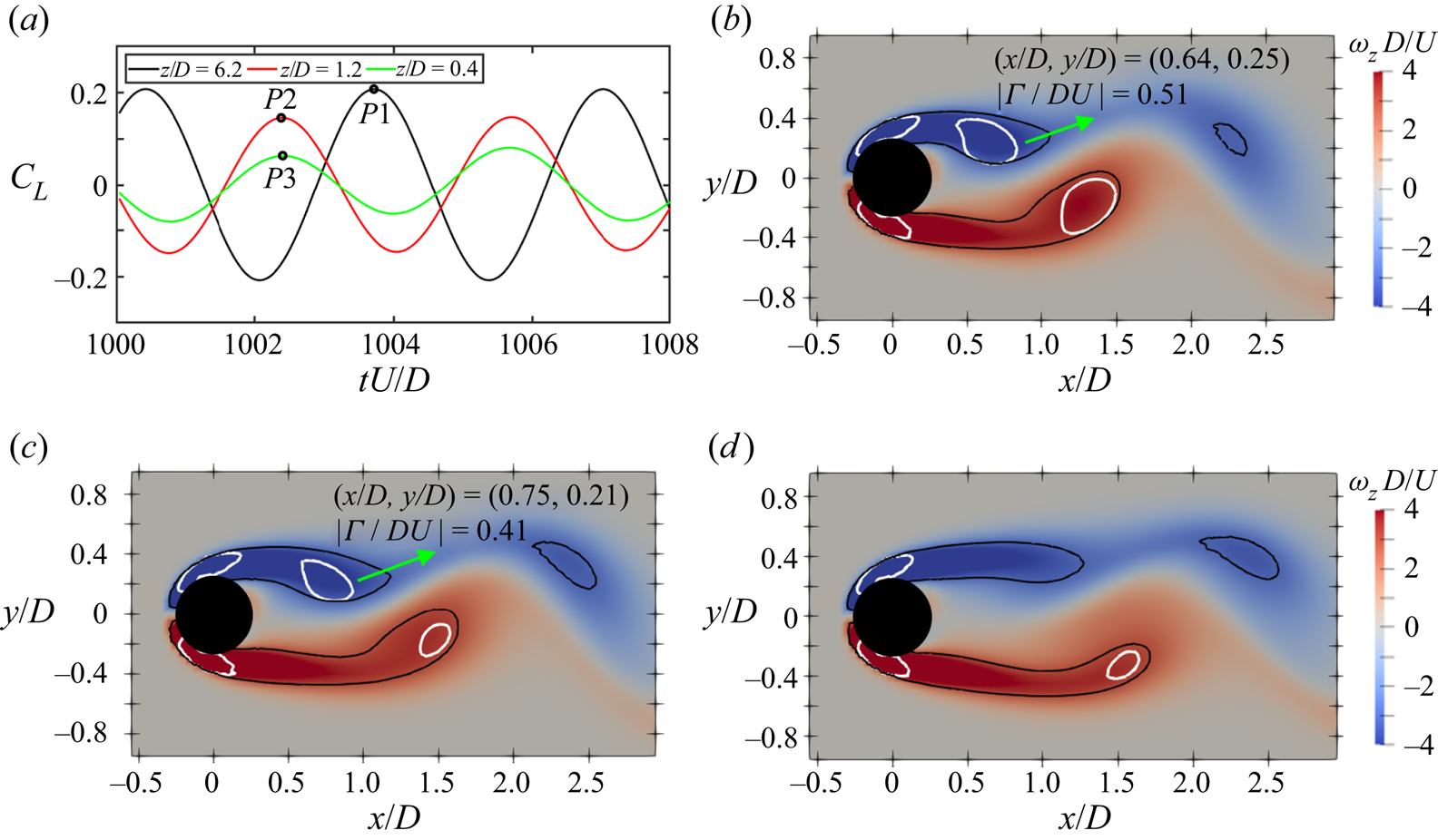
Figure 18. (a) The time history of  $C_L$ is shown at
  $z/D=6.2$ (black), 1.2 (red) and 0.4 (green). (b) The instantaneous spanwise vorticity
  $\omega _z$ in the
  $xy$-plane at
  $z/D=6.2$ at the time instant marked by the peak
  $P1$ in panel (a). (c) Same as panel (b) but in the
  $xy$-plane at
  $z/D=1.2$ at the time instant marked by the peak
  $P2$ in panel (a). (d) Same as panel (b) but in the
  $xy$-plane at
  $z/D=0.4$ at the time instant marked by the peak
  $P3$ in panel (a). The shape of the concentrated
  $\omega _z$ region is shown by the black isoline of
  $\omega _z = \pm 3$. The vortex strength is integrated within the white isoline
  $\lambda _2=-1.7$.
Along the large cylinder, figure 17(a) shows that  $\overline {C'_{L}}$ first decreases from
  $z/D=-20$ to the local minimum point
  $EX_{LL1}$ (
 $z/D=-5$), and increase slightly to the local maximum point
  $EX_{LL2}$; then,
  $\overline {C'_{L}}$ decreases sharply closer to the step. The non-monotonic variation of
  $\overline {C'_L}$ is caused by two different vortex dislocations, i.e. the vortex dislocation between the S- and N-cell vortices (SN-dislocation) and the vortex dislocation between the N- and L-cell vortices (NL-dislocation). Figure 16(c) shows the time history of
  $C_L$ at
  $z/D=-15$ (black),
  $z/D=-5$ (red),
  $z/D=-3.2$ (green) and
  $z/D=-0.7$ (blue). The red thick line on the time axis marks the time interval when the NL-dislocation occurs. Due to the effect of vortex dislocation on
  $C_L$ (as discussed in § 4.1), the black and red curves in figure 16(c) show that the fluctuation amplitude of
  $C_L$ at
  $z/D=-5$ (where the NL-dislocations occur as shown in figure 8a) is smaller than that at
  $z/D=-15$ when vortex dislocation occurs, but is comparable to that at
  $z/D=-15$ when there is no vortex dislocation. Thus, a decrease of
  $\overline {C'_L}$ appears when we move from
  $z/D=-20$ to
  $-5$.
$-5$.
As  $EX_{LL2}$ is approached from
  $EX_{LL1}$, the NL-dislocation effect decreases while the SN-dislocation effect becomes important. In the region between
  $EX_{LL1}$ and
  $EX_{LL2}$, the increased SN-dislocation effect is not strong enough to compensate for the decreased NL-dislocation effect, leading to an increase of
  $\overline {C'_L}$, as shown in figure 17(a). The red and green curves in figure 16(c) show that the oscillation amplitude of
  $C_L$ at
  $z/D=-3.2$ (
 $EX_{LL2}$) becomes larger than that at
  $z/D=-5$ (
 $EX_{LL1}$) when the vortex dislocations occur (indicated by the red thick line on the time axis). As the step is further approached, the effect of SN-dislocations dominates the flow, causing
  $\overline {C'_L}$ to decrease towards the step, as shown in figure 17(a). Since the S-N vortex dislocation occurs in every shedding period of the N-cell vortex (as shown in figure 4a), the oscillation amplitude of
  $C_L$ on the large cylinder in the vicinity of the step will be small and not increase to a large value even when there is no N-L vortex dislocation (e.g.
  $C_L$ at
  $z/D=-0.7$ shown by the blue curve in figure 16c). This leads to a sharp decrease of
  $\overline {C'_L}$ from
  $EX_{LL2}$ towards the step.
5. The effect of diameter ratio on the structural load
Numerical simulations for  $D/d=2.4$ and 2.8 with
  $Re_D=150$ are conducted to investigate the effect of
  $D/d$ on the structural load along the step cylinder. Figure 19(a,c) shows
  $\overline {C_D}$ and
  $\overline {C'_L}$ along the cylinder axis, while figure 19(b,d) shows the contribution from the pressure and skin friction to
  $\overline {C_D}$ and
  $\overline {C'_L}$. For all
  $D/d$, the variations of
  $\overline {C_D}$ and
  $\overline {C'_L}$ are attributed primarily to the pressure. As for
  $D/d=2.0$, four local extremes (
 $EX_{DS}$,
  $EX_{DL}$,
  $EX_{LL1}$ and
  $EX_{LL2}$) are observed for all cases, as denoted in figure 19(a,c). It appears that an increase of
  $D/d$ does not fundamentally change the qualitative distribution of
  $\overline {C_D}$ and
  $\overline {C'_L}$ along the step cylinder but only gradually amplifies the variations of
  $\overline {C_D}$ and
  $\overline {C'_L}$. Since an increase of
  $D/d$ does not cause any abrupt changes in flow characteristics, the amplification mechanism will be discussed based on comparisons between
  $D/d=2.0$ and
  $D/d=2.8$ cases, knowing that the wake at
  $D/d=2.4$ falls in between.

Figure 19. The distribution of structural loads in the  $D/d=2.0$, 2.4 and 2.8 cases are sketched in black, red and green, respectively. (a) The spanwise distribution of the total drag coefficient (
 $\overline {C_D}$); (a i) a close up of (a) at the black dotted rectangle; (b) the spanwise distribution of the viscous (
 $\overline {C_{Df}}$) and pressure (
 $\overline {C_{Dp}}$) drag coefficients; (c) the spanwise distribution of the root mean square of drag coefficient (
 $\overline {C'_L}$); (d) the spanwise distribution of the viscous (
 $\overline {C'_{Lf}}$) and pressure (
 $\overline {C'_{Lp}}$) lift coefficients. In (a,c), the local extremes are marked in all three cases.
Along the small cylinder, the overall increase of  $\overline {C_D}$ shown in figure 19(a) and the overall decrease of
  $\overline {C'_L}$ shown in figure 19(c) are mainly caused by the decreased
  $Re_d$ as
  $D/d$ increases. The increasing pressure difference between the small and large cylinder wakes (due to the larger difference in the Reynolds number between the small and large cylinders) induces a higher increasing rate of
  $\overline {C_D}$ as
  $EX_{DS}$ is approached for the larger
  $D/d$ case, as shown in figure 19(a).
Along the large cylinder, figure 19(a) shows that the increased pressure difference (as described in the previous paragraph) causes the value of  $EX_{DL}$ to decrease as
  $D/d$ increases. As the step is approached from
  $EX_{DL}$ on the large cylinder, a sharper increase of
  $\overline {C_D}$ is observed for larger
  $D/d$ than for smaller
  $D/d$. This is related to an upstream movement of the circulation centre, as discussed previously in § 4.1 and shown in figure 14. Figure 20 shows the streamlines around the large cylinder in the
  $xy$-plane at
  $z/D=-20$,
  $z/D=-1.7$ and
  $z/D=-0.2$ for
  $D/d=2.8$. It is observed that the circulation centre moves 55 % upstream towards the large cylinder (i.e. from
  $x/D=1.86$ at
  $z/D=-1.7$ to
  $x/D=0.83$ at
  $z/D=-0.2$), which is larger than the 29 % upstream movement observed for
  $D/d=2.0$ in figure 14(b,c). This is because the recirculation length behind the small cylinder decreases as
  $D/d$ increases, while the recirculation length behind the large cylinder remains nearly the same in the region far from the step, since
  $Re_D$ remains constant while
  $Re_d$ varies. Thus, as the wake flows behind the small and large cylinders are mixed in the vicinity of the step (as discussed in § 3), the recirculation length behind the large cylinder becomes smaller for
  $D/d=2.8$ than for
  $D/d=2.0$ (as shown in figure 6c,d), leading to a larger upstream movement of the circulation centre for
  $D/d=2.8$ also.

Figure 20. The time-averaged streamlines for  $D/d=2.8$ on the
  $xy$-plane: (a) at
  $z/D=-20$; (b) at
  $z/D=-1.7$; (c) at
  $z/D=-0.2$. The location of the circulation centre is marked by the red line.
Figure 19(c) shows that both  $EX_{LL1}$ and
  $EX_{LL2}$ decreases as
  $D/d$ increases. This is because the effect of the NL vortex dislocation on
  $\overline {C'_L}$ (as shown in figure 17(a) and discussed in § 4.3) is amplified, since the number of vortex dislocations and their duration for a given time interval increase as
  $D/d$ increases (this can be observed by comparing figure 16(a) and figure 21; the corresponding mechanism has been discussed in Tian et al. Reference Tian, Jiang, Pettersen and Andersson2020a). Figure 21 shows the time history of the cross-flow velocity contours for
  $D/d=2.8$ showing nine occurrences of vortex dislocations. During the same time interval, eight series of vortex dislocations for
  $D/d=2.0$ are shown in figure 16(b). Moreover, the duration of each vortex dislocation (indicated by the thick red lines in figure 16(b) and figure 21) increases from 11
  $D/U$ for
  $D/d=2.0$ (containing 2 N- and 4 L-cell vortices) to 17
  $D/U$ for
  $D/d=2.8$ (containing 4 N- and 6 L-cell vortices). This further strengthens the effect of vortex dislocations on
  $\overline {C_D}$ shown in figure 12(a) as previously discussed in § 4.3. As a result,
  $\overline {C_D}$ decreases less for larger
  $D/d$ than for smaller
  $D/d$ in the region
  $-8< z/D<-5$, as shown in figure 19(a i) (a close-up of figure 19a).

Figure 21. Cross-flow velocity component  $v$ as a function of the non-dimensional time, along spanwise sampling line at
  $(x/D, y/D)=(0.6, 0)$ for
  $D/d=2.8$. The red thick line highlights the position where vortex dislocations occur.
The investigations in this section indicate that our discussions and conclusions in § 4 are likely valid not only for the step cylinder  $D/d=2$ case but also for other
  $D/d$ cases. An increase in diameter ratio strengthens the effect of vortex dislocation and the three-dimensional effect (induced by the step) in the cylinder wakes, thereby further amplifying the variation of the structural load over the step cylinder.
6. Conclusion
The flow and the structural load along a step cylinder with diameter ratios  $D/d=2.0$, 2.4 and 2.8 are investigated at
  $Re_D=150$ based on DNS. Our results agree well with previous studies (Dunn & Tavoularis Reference Dunn and Tavoularis2006; Morton & Yarusevych Reference Morton and Yarusevych2010; Tian et al. Reference Tian, Jiang, Pettersen and Andersson2020Reference Tian, Jiang, Pettersen and Anderssona,Reference Tian, Jiang, Pettersen and Anderssonb), for the three dominating spanwise vortices, i.e. the S-, N- and L-cell vortices, vortex dislocations occurring at the S-N and N-L cell boundaries as well as the non-parallel shedding of the S- and L-cell vortices. In addition, the numerical results provide a more in-depth understanding of the non-parallel shedding of the S-cell vortex, the variation of the structural load and the vortex dislocation effect on the structural load.
The different formation mechanisms of the non-parallel shedding in the S- and L-cell regions were discussed. The non-parallel shedding in the L-cell region belongs to the conventional oblique vortex shedding (Williamson Reference Williamson1989). However, the scenario is different for the S-cell vortex. As the step is approached along the small cylinder, the S-cell vortex changes from parallel shedding to non-parallel shedding but keeps the shedding frequency unchanged. This uncommon non-parallel shedding phenomenon is referred to as non-uniform oblique shedding in the present work. The underpinning mechanism is that the downwash flow behind the small cylinder (caused by the pressure difference between the small cylinder wake and large cylinder wake) and the extended recirculation length (caused by blending of the wake behind the small and large cylinder) induce an increase of the production rate of the S-cell vortex strength and a farther downstream movement of the S-cell vortex formation position as the step is approached along the small cylinder. This leads the part of the S-cell vortex in the vicinity of the step to form farther downstream compared with the part of the S-cell vortex away from the step, despite the same shedding frequency. Thus, the non-uniform oblique shedding appears in the S-cell region.
Additionally, we analysed the influence of the vortex dynamics on the structural load. First, the effect of vortex dislocations on the structural load was studied based on the investigation of the vortex shedding pattern during the vortex dislocation processes and the time history of the corresponding drag ( $C_D$) and lift (
 $C_L$). We found that a major reduction (90 %) of the sectional lift amplitude and a relatively modest reduction (5.7 %) of the sectional drag amplitude are caused by the decreased circulation and the weakened staggered Kármán vortex shedding pattern when vortex dislocations occur, where the latter effect plays the major role. This new understanding of the effect of vortex dislocations on the structural load provides an explanation for the formation of the local minimum
  $EX_{LL1}$ (caused by the NL-dislocation effect) as well as the sharp decrease of
  $\overline {C'_L}$ in the vicinity of the step at the small (caused by the SN-dislocation effect) and the large cylinder (caused by the NL-dislocation effect). From
  $EX_{LL1}$ to the step, since the SN-dislocation effect is not strong enough to compensate for the decreased NL-dislocation effect, a local maximum
  $EX_{LL2}$ appears. Although the vortex dislocation effect on the structural load has been observed before, we provide the first in-depth investigation of it.
Besides the vortex dislocation effect, the diameter ratio  $D/d$ causes the pressure and wakes behind the small and large cylinders to be distinctly different in the region far away from the step; and such difference decreases as the step is approached due to the mixing of the small and large cylinder wakes. Under this process, for the small cylinder, the base suction and the recirculation length increase as the step is approached. The first one causes an increase of
  $\overline {C_D}$ along the small cylinder until the local maximum
  $EX_{DS}$ is reached. The second one, together with the vortex dislocation effect, induces a sharp decrease of
  $\overline {C_D}$ from
  $EX_{DS}$ to the step. For the large cylinder, the base suction decreases as the step is approached. This plays a major role in the decrease of
  $\overline {C_D}$ as the step is approached, before reaching the local minimum
  $EX_{DL}$. As the step is further approached from
  $EX_{DL}$, the recirculation length decreases and the base suction increases, leading to an increase of
  $\overline {C_D}$ from
  $EX_{DL}$ close to the step.
In § 5, the robustness of our discussions and conclusions is justified by investigating the wake flow and structural load for  $D/d=2.4$ and 2.8. Increasing
  $D/d$ is found to amplify the variation of the structural load along the step cylinder, since it strengthens not only the three-dimensional effect of the cylinder wakes caused by
  $D/d$ but also the effect of vortex dislocation.
Although all investigations in the present paper are based on step cylinders with  $D/d=2.0$, 2.4 and 2.8 at Reynolds number
  $Re_D=150$, the three dominating spanwise vortices (S-, N- and L-cell vortices) and the vortex dislocation between them were also observed in other step cylinder cases with
  $1.55< D/d<2$ at
  $67< Re_D<3900$ (Norberg Reference Norberg1992; Dunn & Tavoularis Reference Dunn and Tavoularis2006; Tian et al. Reference Tian, Jiang, Pettersen and Andersson2021). As long as the above-mentioned two flow features exist, we believe that the variation of the structural load and the mechanism underpinning the effect of vortex dislocations on the structural load reported in the present study could also exist for the step cylinder cases with other diameter ratios and at higher Reynolds numbers, at least until transition occurs in the shear layer. We believe that our discussions and conclusions can shed light on other bluff body wakes that contain several adjacent spanwise vortices and three-dimensional flow effects caused by body shapes, for example, flow around a free-end cylinder, a curved cylinder and a tapered cylinder.
Funding
Computing resources were granted by the Norwegian Research Council (Program for Supercomputing) under projects nn9191k and nn9352k.
Declaration of interests
The authors report no conflict of interest.
Appendix A. Grid convergence and spanwise length convergence
Since the complex wake flow is mainly caused by the changed diameter at the step of the cylinder, the most critical case is expected to appear when  $D/d=2.8$ (i.e. the largest diameter ratio used in this work). Both the grid convergence and the spanwise length convergence study are conducted based on a step cylinder with
  $D/d=2.8$. Table 1 shows an overview over all the numerical simulations conducted in the present work. The three cases denoted Coarse, Medium and Fine-28A are selected for the grid convergence study. For the spanwise convergence study, the Fine-28A, Fine-28B and Fine-28C cases are used.
A.1. Grid convergence
Table 3 shows the Strouhal number ( $St$) of the three dominating vortex cells (
 $St_S = f_S D/U$,
  $St_N = f_N D/U$ and
  $St_L = f_L D/U$) calculated by discrete Fourier transform of the time series of the streamwise velocity
  $u$ along a vertical sampling line at
  $(x/D, y/D)=(0.6, 0.2)$ in the Coarse, Medium and Fine-28A cases. Only tiny differences can be observed for
  $St_N$ and
  $St_L$ in these three cases. For
  $St_S$, a clear convergent tendency can be seen as the grid resolution increases; the difference between the finest two cases (Medium and Fine-28A) is only 0.3 %. It should be noticed that, due to the diameter ratio
  $D/d$,
  $St_S$ is more sensitive to the grid refinement than
  $St_N$ and
  $St_L$.
Table 3. The Strouhal number ( $St$) of three dominating vortex cells (
 $St_S = f_S D/U$,
  $St_N = f_N D/U$ and
  $St_L = f_L D/U$) for the three cases with
  $D/d=2.8$, i.e. Coarse, Medium and Fine-28A, as shown in table 1. By means of the empirical
  $St_S=(0.2663-1.019/Re_d^{0.5})\times 2.8$ from Norberg (Reference Norberg2003), the empirical Strouhal number of the S-cell vortex (
 $St_{S}$) is calculated and shown in the fifth row.
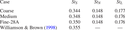
Figure 22(a) shows the time-averaged streamwise velocity above the step at  $(x/D, y/D)=(-0.4, 0)$. A close up of the red rectangle in figure 22 is shown in figure 22(a i). Figure 23(a,b) displays the spanwise distribution of the time-averaged drag coefficient (
 $\overline {C_D}$) and the time-averaged fluctuation of the lift coefficient (
 $\overline {C'_L}$), respectively. Both figures 22 and 23 clearly show a convergent tendency from the case Coarse to the case Fine-28A. The difference between Medium and Fine-28A is negligible. According to the above careful comparisons, it can be concluded that the grid resolution in the Fine-28A case is sufficiently fine to accurately simulate the flow around the step cylinders discussed in the present paper.

Figure 22. Distributions of time-averaged streamwise velocity  $\bar {u}/U$ along a sampling line AB in the
  $xz$-plane at
  $y/D=0$ in the
  $D/d=2.8$ case. Inset: (a i) a zoomed-in view of the upper part of the curves (red rectangle); (a ii) a sketch of the position of the sampling line AB of a length 0.8
 $D$ at
  $x/D=-0.4$.

Figure 23. Distribution of time-averaged force coefficients in the three  $D/d=2.8$ cases with different grid resolutions: (a) drag coefficient
  $\overline {C_D}$, (b) lift coefficient
  $\overline {C'_L}$. Inset: (a i) a zoomed-in view of the curves marked by the red rectangle in panel (a). The rectangle and cross are the drag coefficients corresponding to the Reynolds number 50 and 55, obtained from Rajani et al. (Reference Rajani, Kandasamy and Majumdar2009).
A.2. Spanwise length convergence
Besides the grid convergence, the spanwise length convergence was also examined by using the same grid structures as in Fine-28A, and changing the lengths of both the large ( $L$) and small (
 $l$) cylinders (see table 1). Figure 24 shows the spanwise distributions of
  $\overline {C_D}$ and
  $\overline {C'_L}$ in the region
  $-20< z/D<10$. The results indicate that the free-slip wall boundary condition at the top and bottom of the computational domain has relatively strong effects on the results in the Fine-28B case. Especially at
  $z/D=-20$, which is close to the bottom boundary (
 $z/D=-23.96$) for Fine-28B,
  $\overline {C_D}$ and
  $\overline {C'_L}$ in Fine-28A and Fine-28C are approximately 10 % larger than those in Fine-28B. The difference between the black (Fine-28C) and red dotted (Fine-28A) curves is minimal. The spanwise variation of the angle of the S-cell vortex tubes (
 $\alpha _S$) in the three
  $D/d=2.8$ cases with different spanwise lengths is shown in figure 25. Due to the free-slip boundary condition at the top of the computational domain (as described in § 2),
  $\alpha _S$ becomes zero as the top is approached. The significantly lower
  $\alpha _S$ at
  $6< z/D<11$ for Fine-28B than in the other two cases reflects the strong influence of the upper boundary condition on the distribution of
  $\alpha _S$. For Fine-28A and Fine-28C, however, the shedding angles
  $\alpha _S$ almost coincide for
  $z/D<10$. This suggests that the vortex dynamics in the vicinity of the step is practically unaffected by the boundary conditions as long as the spanwise domain
  $L_z=L+l>45D$. From the discussions in this section, we are convinced that the spanwise length in the Fine-28A and Fine-28C cases converge well in the flow field
  $-20< z/D<10$ for the analysis and discussions the present paper focused.

Figure 24. Distribution of time-averaged force coefficients in the three  $D/d=2.8$ cases with different spanwise lengths: (a) drag coefficient
  $\overline {C_D}$, (b) lift coefficient
  $\overline {C'_L}$.

Figure 25. Spanwise variation of the angle  $\alpha$ of the vortex tubes in the S-cell region (
 $z/D>2.5$) in the three
  $D/d=2.8$ cases with different spanwise lengths.
A.3. Comparison with previous studies
It was observed that, although a non-uniform oblique shedding appears in the S-cell region, the shedding frequency of the S-cell vortex is barely influenced (detailed discussions were addressed in § 3). This makes it reasonable to use an empirical formula to validate our  $St_S$. Table 3 shows that, as the grid resolution is improved, the difference between
  $St_S$ in the present simulations and the empirical value (Williamson & Brown Reference Williamson and Brown1998) decreases; this difference is smaller than 1 % for Fine-28A. In addition, we obtained time-averaged drag coefficients at
  $Re= 50$ and 55 from Rajani et al. (Reference Rajani, Kandasamy and Majumdar2009) and display them in figure 23(a i). For
  $D/d=2.8$,
  $Re_d$ (the Reynolds number for the small cylinder) is 53.5. Therefore, it is reasonable to observe that
  $\overline {C_D}$ on the small cylinder part far from the step is between the drag coefficients for
  $Re_D=50$ (the rectangle in figure 23a i) and for
  $Re_D=55$ (the cross in figure 23a i).
In general, based on the results presented in this section, we conclude that the configuration and mesh used in the Fine-B case (see table 1) are sufficiently good for reliable DNS simulations in the present study.


 Open access