


1. Introduction
Viscous gravity currents are near-horizontal, low-Reynolds-number flows driven by buoyancy. They are a canonical flow structure occurring broadly in natural phenomena such as lava flows and glaciers as well as various industrial applications such as the pouring of cement. They have received extensive study in numerous configurations since the seminal work of Huppert (Reference Huppert1982).
Here we consider the flow of such a gravity current atop a deformable granular medium. Several significant new features are possible in this case. At the grain scale, the viscous fluid can infiltrate the granular medium in a manner similar to a porous medium, although with additional behaviours because of the potential for granular rearrangement. At the continuum scale, the viscous fluid can cause the entire granular layer to flow, with potential feedback on the dynamics of the gravity current. This effect is the focus of our study. Our particular motivation is to the formation of massive sulphide ores in magmatic systems, but it also has broader application, for example in the reworking of subglacial tills and potentially the formation of moraines.
Sulphide-rich liquid forms a small  ${\lesssim }1\,\%$ fraction of basaltic magmas (Tonnelier Reference Tonnelier2010). This liquid is significantly heavier than the dominant silicate melt and significantly less viscous. It is thought to be transported as small droplets in active magmatic systems before being deposited at various concentrations as the system cools (Robertson, Barnes & Le Vaillant Reference Robertson, Barnes and Le Vaillant2016). It is one of the last components to solidify and hence is thought to interact with granular mushes of silicate crystals. Because various metallic components (especially nickel, cobalt, copper and platinum-group elements) are preferentially absorbed by these droplets during active transport, they form valuable ores when deposited in sufficiently high concentration (Campbell & Naldrett Reference Campbell and Naldrett1979; Kiseeva & Wood Reference Kiseeva and Wood2015; Barnes et al. Reference Barnes, Mungall, Le Vaillant, Godel, Lesher, Holwell, Lightfoot, Krivolutskaya and Wei2017). Hence a focus of economic geology is finding such locations. The classical picture is that the heavier sulphides migrate to the bottom of the system (Naldrett Reference Naldrett1973). However, Chung & Mungall (Reference Chung and Mungall2009) argued that this picture is incomplete and that the very low wettability of silicate crystals to sulphide liquid can prevent the percolation of moderately sized droplets through the mush. Here we explore whether massive sulphides could form atop a granular mush; see figure 1(a).

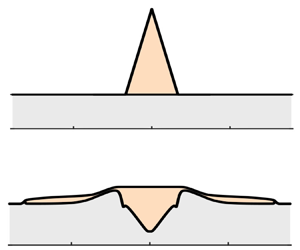
Figure 1. Schematic of the flow set-up. (a) The liquid sulphide and silicate crystals sink within the silicate melt. Thin layers of liquid sulphide may not percolate due to its low wettability. (b) Model set-up: a viscous gravity current spreads atop a granular layer.
Specifically, we consider the spread of a very viscous Newtonian fluid above a granular layer modelled as a dense shallow continuum with a  $\mu (I)$-rheology (GDR-MiDi 2004; Gray & Edwards Reference Gray and Edwards2014). A key characteristic of this rheology is a yield criterion below which the granular layer is ‘rigid’, analogous to a viscoplastic material. The
  $\mu (I)$-rheology has been able to accurately capture many experimental observations including avalanching, silo discharge and bulldozing (Da Cruz et al. Reference Da Cruz, Emam, Prochnow, Roux and Chevoir2005; Kamrin & Koval Reference Kamrin and Koval2012; Sauret et al. Reference Sauret, Balmforth, Caulfield and McElwaine2014; Staron, Lagrée & Popinet Reference Staron, Lagrée and Popinet2014). Whilst there has been much research on gravity-driven dense granular flows, and some investigation of their capacity to erode an underlying substrate (Viroulet et al. Reference Viroulet, Edwards, Johnson, Kokelaar and Gray2019), the coupled interaction of a viscous gravity current with a granular layer has not previously been studied. We focus on the case where the viscous liquid does not infiltrate the granular pack; see figure 1. This is possible if the grains are non-wetting to the viscous liquid and the liquid layer is relatively thin so that its excess hydrostatic pressure does not exceed the capillary entry pressure of the granular pore space. We develop a novel but simplified isothermal model that captures the dominant flow physics on relatively short time scales with the displacement of the ambient silicate melt having a negligible influence on the flow (Huppert Reference Huppert1982).
We describe the model and generic results in §§ 2 and 3. We return to the question of massive sulphides in § 4.
2. Shallow two-layer model
The set-up is shown in figure 1(b). The two phases are modelled as continua lying on a horizontal layer of impermeable country rock. As discussed in § 1, the sulphide droplets are non-wetting to the crystals and we assume that the granular layer is impermeable to the liquid (noting that penetration could occur if the liquid layer was very thick so that the hydrostatic pressure exceeds the capillary entry pressure; we revisit this assumption in § 4). The thickness of the viscous liquid is denoted by  $h_u(x,t)$ whilst the thickness of the granular layer is denoted by
  $h_l(x,t)$, with the total thickness given by
  $H(x,t)=h_u+h_l$, where
  $x$ is the horizontal coordinate and
  $t$ is time. We restrict our attention to a two-dimensional geometry with the vertical coordinate denoted by
  $z$. The flow is driven predominantly by the weight of the layers and inertia is negligible. For simplicity, the two layers are taken to have the same excess density relative to the ambient melt,
  $\Delta \rho$ (the density of the granular layer is the product of the grain density with the solid volume fraction). The case of a density difference between the layers does not qualitatively change the results; for further discussion, see § 4. The viscous liquid is assumed to be Newtonian with dynamic viscosity
  $\eta$ and the granular layer has a
  $\mu (I)$-rheology described below. There is no slip at the interface between the layers and the stress is continuous. Initially, the granular layer has uniform thickness
  $h_l(x,0)=L$ and the upper layer is a localised deposit whose shape is an input to the model that we vary.
The flow is assumed to be predominantly in the horizontal direction so that the pressure is hydrostatic across both layers:
 \begin{equation} p=\Delta \rho g (H-z), \end{equation}
where g is earth's gravity. Momentum balance implies that the shear stress in both layers is given by
 \begin{equation} \tau =-(H-z) \Delta \rho g \frac{\partial H}{\partial x}, \end{equation}
where we have used the condition of zero shear stress at the free surface  $z=H(x,t)$. The constitutive model for the granular layer is provided by (GDR-MiDi 2004)
 \begin{equation} \tau = \mu(I) p \operatorname{sgn} \left( \frac{\partial u}{\partial z} \right)\quad \text{where} \ I = \left\vert \frac{ \partial u}{\partial z} \right\vert \sqrt{m/p}, \end{equation}
where u is the horizontal velocity and m is the grain mass (per unit length into the page in figure 1). This  $\mu (I)$-rheology is defined by the relationship between the effective friction coefficient
  $\mu$ and the inertial number
  $I$ (GDR-MiDi 2004). We use the following linearised relationship: (Da Cruz et al. Reference Da Cruz, Emam, Prochnow, Roux and Chevoir2005; Kamrin & Koval Reference Kamrin and Koval2012)
 \begin{equation} I=\frac{max (0,\mu-\mu_s)}{b}, \end{equation}
where  $\mu _s$ is the minimum slope gradient for which flow occurs, and
  $b$ is a dimensionless constant. The granular material is rigid when
  $\mu < \mu _s$. Relating (2.1) and (2.2) with (2.3a) implies that
  $\mu (I)$ is constant across the granular layer and given by the magnitude of the free-surface gradient, (see also Gray & Edwards Reference Gray and Edwards2014)
 \begin{equation} \mu=\left\vert \frac{\partial H}{\partial x} \right\vert. \end{equation}
Equations (2.3b) and (2.4) combined with no slip at the base  $z=0$ then furnishes a Bagnold velocity profile in the lower layer (Bagnold Reference Bagnold1954),
 \begin{equation} u_l(x,z,t) =-\frac{2 \sqrt{\Delta \rho g}}{3 b \sqrt{m}} [H^{3/2} - (H-z)^{3/2} ] \mathcal{F} \left(\frac{\partial H}{\partial x} \right), \end{equation}
where
 \begin{equation} \mathcal{F}\left(\frac{\partial H}{\partial x} \right)= \operatorname{sgn}\left(\frac{\partial H}{\partial x} \right) max \left(0,\left\vert\frac{\partial H}{\partial x}\right\vert-\mu_s \right). \end{equation}
The volume flux in each layer is given by
 $$\begin{gather} Q_l(x,t) =- \frac{2\sqrt{\Delta\rho g}}{15 b \sqrt{m}} [(h_u+h_l)^{3/2} (3h_l - 2h_u) + 2 h_u^{5/2} ] \mathcal{F} \left(\frac{\partial H}{\partial x} \right), \end{gather}$$
 $$\begin{gather}Q_u(x,t) =-\frac{2\sqrt{\Delta\rho g}}{3 b \sqrt{m}} [(h_u+h_l)^{3/2} h_u - h_u^{5/2} ]\mathcal{F} \left(\frac{\partial H}{\partial x} \right) -\frac{\Delta\rho g}{3 \eta} h_u^3 \frac{\partial H}{\partial x}. \end{gather}$$
The last term in the upper layer flux,  $Q_u$, arises from its own viscous shearing.
We non-dimensionalise the system by scaling all lengths with the initial thickness of the granular layer,  $L$, and by scaling time
  $t$ with the time scale
  $T_g$ for granular shearing,
 \begin{equation} T_g = \frac{3b\sqrt{m}}{\sqrt{\Delta\rho g L}}. \end{equation}
Henceforth all variables are dimensionless. The dimensionless volume flux in each layer is given by
 $$\begin{gather} Q_l(x,t) =- \frac{2}{5} [(h_u+h_l)^{3/2} (3h_l - 2h_u) + 2 h_u^{5/2} ] \mathcal{F} \left(\frac{\partial H}{\partial x} \right), \end{gather}$$
 $$\begin{gather}Q_u(x,t) =-2 [(h_u+h_l)^{3/2} h_u - h_u^{5/2} ]\mathcal{F} \left(\frac{\partial H}{\partial x} \right) -\alpha h_u^3 \frac{\partial H}{\partial x}, \end{gather}$$
where
 \begin{equation} \alpha=\frac{b \sqrt{m L \Delta \rho g}}{\eta}, \end{equation}
is a dimensionless number that relates the granular ‘viscosity’ to the viscosity of the upper layer,  $\eta$. The flow is governed by two dimensionless parameters:
  $\mu _s$ and
  $\alpha$. Mass conservation in each layer is written as
 \begin{equation} \frac{\partial h_i}{\partial t} + \frac{\partial Q_i}{\partial x}=0, \quad \text{for} \ i=u,l. \end{equation}
3. Results
The two coupled partial differential equations for the flow thicknesses (2.14) are integrated numerically using a finite-difference scheme; for details, see Appendix A. In the case that  $|\partial H/\partial x| \leq \mu _s$ everywhere initially, the lower layer does not yield (except possibly in a very small neighbourhood of the contact point with the granular material). The upper layer spreads predominantly as a classical viscous gravity current over a rigid bed (Huppert Reference Huppert1982). Henceforth, we only consider initial conditions with
  $max |\partial H/\partial x| > \mu _s$.
The numerical results for a particular choice of parameters and initial condition are shown in figure 2. This example illustrates the general and important features of the flow. The evolution of the system can generally be broken into four stages, which we outline here, with the full details provided in the following subsections. Initially, the gradients in the thickness of the upper layer induce yielding in the lower layer. There is a fast transient with the lower layer eroded to form granular levees (stage 1, figure 2(c); § 3.1). This stage ends as the free-surface gradient approaches  $\mu _s$ and the granular shearing slows. Next, the flow is driven by the much slower slumping of the viscous deposit. There is further erosion and the growing levees are pushed outwards by the gravity-driven viscous flow (stage 2, figure 2(d); § 3.2). Subsequently, the outward viscous flux diminishes and is unable to continue pushing the entire levee. The stress is reduced and yielding occurs only near the top of the levee, which breaks away (stage 3, figure 2(e); § 3.3). Finally, the top part of the levee is very slowly pushed horizontally by the viscous liquid. The new levee gradually diminishes in size and the viscous deposit becomes segregated with a central portion trapped by the rigid remnant of the original levee (stage 4, figure 2(f); § 3.4).

Figure 2. Stages of the containment of viscous liquid atop a granular layer (with  $\mu _s=0.25$ and
  $\alpha =1$). (a) Set-up. (b) Initial configuration (
 $t=0$). (c) Stage 1: levee formation (
 $t=0.1$). (d) Stage 2: viscous pushing of the levee (
 $t=50$). (e) Stage 3: break-off of the top part of the levee (
 $t=1000$). (f) Stage 4: separation and containment of viscous liquid (
 $t=100\ 000$).
3.1. Stage 1: initial erosion and levee formation
The initial transient (stage 1) is shown in figure 3. The gradients in the free surface are sufficient to yield the granular material underlying the viscous deposit. This causes the granular material there to flow outwards. Beyond the viscous deposit, the granular material is approximately rigid (its motion is slow relative to the deformation of material beneath the liquid). The mass eroded below the viscous deposit is transferred into levees at either side. In stage 1, the volume flux in the upper layer is negligible relative to that in the lower layer because the upper layer is relatively thin. Hence the thickness of the upper layer is approximately constant during the initial transient; almost all motion arises from the yielding of the granular material.

Figure 3. Stage 1: fast initial erosion of the granular layer and levee formation with  $\alpha =1$ and
  $\mu _s=0.25$. Viscous deposit and levee shape (calculated numerically) at (a)
  $t=0$, (b)
  $t=0.01$ and (c)
  $t=0.1$; the dotted blue line shows
  $|\partial H/\partial x| \approx \mu _s$ for which the granular layer becomes quasi-rigid (3.1). (d) Location of the front of the levee (black line) and the quasi-rigid location (red dashed line). (e,f) Thicknesses at
  $t=0.1$ for (e)
  $\mu _s=0,0.125,0.25,0.375$ with
  $\alpha =1$ and (f) with
  $\alpha =0.04, 0.2, 1, 5, 25$ and
  $\mu _s=0.25$.
The fast granular mass transfer continues until the free-surface gradient approaches the yield point,  $|\partial H/\partial x| \approx \mu _s$, and the granular layer slows, becoming quasi-rigid. Stage 1 ends with the free surface having the shape
 \begin{equation} H=\mu_s(x_f-|x|) + 1, \end{equation}
for  $|x|< x_f$, where volume conservation implies that
  $x_f=\sqrt {V/\mu _s}$ for a viscous deposit of volume
  $V$ (per unit length into the page). The shape (3.1) is shown as a blue dotted line in figure 3(c), accurately capturing the numerically integrated shape at
  $t=0.1$. The evolution of the edge of the levee,
  $\pm x_c(t)$, is shown in figure 3(d), with the red dashed line corresponding to
  $x_c=x_f$; the motion of the levee is relatively fast until the yield point is reached. Subsequent stages are much slower as they are driven by the slumping of the viscous liquid.
Different values of the yield gradient,  $\mu _s$, lead to similar behaviour but with a quantitative change in the quasi-rigid shape (3.1) at the end of stage 1; see figure 3(e). The special case of
  $\mu _s = 0$ (red lines in figure 3e) is qualitatively different because there is no quasi-rigid shape and instead the upper free surface gradually relaxes to the horizontal; for further discussion see § 3.2.
The dynamics in stage 1 is largely insensitive to the value of  $\alpha$ because there is little viscous deformation; see figure 3(f). For particularly large
  $\alpha$, there are small changes in the upper layer thickness around
  $x=0$ because there is some outwards viscous deformation at very early times.
3.2. Stage 2: viscous ‘pushing’ of the levee
At the end of stage 1, levees at the edges of the viscous deposit are formed with  $|\partial h_l/\partial x| \approx \mu _s$. Subsequently, in stage 2, the levees slowly move outwards driven by slumping of the viscous deposit; see figure 4. The free-surface gradient of the levees is held just above the yield criterion because the viscous liquid at the edge of the levee just yields the quasi-rigid granular material. Thus the viscous deposit slowly ‘pushes’ the levees outwards. The levees cannot be fully surmounted by the viscous deposit as this would first cause significant yielding in the granular layer, which in turn drives fast outwards flow away from the surmounting viscous liquid as in stage 1. The levees also grow with continued erosion of the lower layer (figure 4).

Figure 4. Stage 2: viscous ‘pushing’ of the levee with  $\alpha =1$ and
  $\mu _s=0.25$. (a–d) Viscous deposit and levee shape at
  $t=1$,
  $4$,
$4$,  $16$,
$16$,  $64$. In (b–d) the blue dashed line shows the shape from (a). (e,f) Thicknesses at
  $t=16$ for (e)
  $\mu _s=0,0.125,0.25,0.375$ with
  $\alpha =1$ and (f) with
  $\alpha =0.04, 0.2, 1, 5, 25$ and
  $\mu _s=0.25$.
The volume flux in the granular layer is continuous across the edge of the viscous deposit and so  $\mu$ is continuous there also, with
  $\mu \approx \mu _s$. For the present case of equally dense fluids, this gives
  $|\partial H/\partial x| \approx \mu _s$ at the edge of the viscous deposit. This condition is adjusted slightly for layers with different densities but the levee is still not surmounted and the qualitative features are unchanged; see § 4.
As in stage 1, different values of  $\mu _s >0$ lead to quantitative changes in the levee slope (see figure 4e) but the qualitative behaviour is unchanged. The exception is the case
  $\mu _s =0$ (red lines in figure 4e) for which the upper interface has become approximately horizontal by
  $t=16$ and the flow is almost entirely arrested. There is subsequently negligible change in the thickness but we note that there would be further slow spreading in the case of a density difference.
In stage 2, the flow is driven by the viscous deformation of the upper liquid layer and so changes in the viscosity ratio,  $\alpha$, predominantly lead to changes in the time scale; see figure 4(f). The flow stages and features are, however, qualitatively similar across different values of
  $\alpha$.
The other interesting feature of this regime is the steepening of the front of the viscous–granular interface at the edge of the viscous deposit; see figure 4(d). This arises because, near the edges of the viscous liquid,  $\partial H/\partial x \approx \pm \mu _s$ and so the flux in the upper layer is
  $Q_u \approx \mp \alpha \mu _s h_u^3$. The mean velocity of the upper layer is proportional to
  $h_u^2$ whilst the lower layer moves much more slowly. Where the viscous liquid is thicker, it travels faster and then incorporates liquid in thinner regions leading to a steepening at the viscous–granular interface. This phenomenon (sometimes referred to as shock formation) has been observed previously in two-layer viscous gravity currents (Dauck et al. Reference Dauck, Box, Gell, Neufeld and Lister2019).
3.3. Stage 3: decaying viscous flux and levee break-off
Stage 2 ends because the flux in the viscous layer diminishes in time and eventually cannot continue to push the entire levee outwards. As the viscous layer slumps, the free-surface gradient reduces. Hence a progressively smaller horizontal width of the granular layer below the viscous deposit is yielded (note that the granular layer is either entirely yielded throughout its thickness or entirely rigid throughout its thickness). The yielded portion is indicated by green bands in figures 5(a) and 5(b). The length  $\mathcal {L}$ of the bands as a function of time is shown in figure 5(c).

Figure 5. Stage 3: decaying viscous flux and levee break-off with  $\alpha =1$ and
  $\mu _s=0.25$. (a,b) Viscous deposit and levee shape at
  $t=4$ and
  $t=64$ (see figure 3), with green bands indicating the region where the lower layer is yielded. (c) Extent of the yielded band,
  $\mathcal {L}$, as a function of time. (d) Shape at
  $t=1000$ showing levee break-off.
Eventually, the only part of the granular layer below the viscous liquid that is yielded is in a small neighbourhood of the levee ( $|\partial H/\partial x| \approx \mu _s$ at the edge of the viscous deposit as discussed above). This initiates stage 3. The viscous liquid only yields the granular material very close to the top of the levee (figure 5b). A smaller levee is broken off from the top of the main levee and is pushed outwards; see figure 5(d). The granular material between the two break-off points is entirely rigid and is stationary for the remainder of the motion.
3.4. Stage 4: containment of a pool of viscous liquid
In the final stage, the smaller broken-off levee continues to be pushed outwards. This smaller levee diminishes in size as it is gradually deposited on the far side of the original levee whilst the viscous flux continues to diminish (see figure 6). The remnant of the original levee, which is entirely rigid, traps a significant proportion of the viscous deposit. The liquid is segregated into a contained pool, whose height gradually decays to the peak of the rigid granular material, and two thin films that are mobile indefinitely but migrate very slowly; see figure 6(b).

Figure 6. Stage 4: containment of a pool of viscous liquid with  $\alpha =1$ and
  $\mu _s=0.25$. (a,b) Viscous deposit and levee shape at
  $t=5000$ and
  $t=100\ 000$.
Figure 7 shows the shape of the viscous deposit and granular material at  $t=5000$ with the initial conditions shown in panels (a) and (d), for two different values of the yield gradient,
  $\mu _s$. The fraction of the viscous deposit that is trapped at late times is also shown. When the yield gradient
  $\mu _s$ is smaller, more of the lower layer is eroded in stage 1, leading to a greater trapped fraction. Similar behaviour occurs for initial viscous deposits with larger free-surface gradient.

Figure 7. (a,d) Initial viscous deposit shape for the two rows. (b,c) Shape of the viscous deposit and levee at  $t=5000$ for
  $\mu _s=0.125$ and
  $\mu _s=0.25$. The percentages indicate the fraction of viscous liquid that is trapped at long times. (e,f) Shape of the viscous deposit and levee as in (b,c) but with the initial shape from (d).
Figure 8(a) shows the trapped fraction as a function of  $\mu _s$ for the two initial shapes in figure 7 in the case that
  $\alpha =1$ (crosses) and
  $\alpha =10$ (circles) (red corresponds to the triangular initial condition and blue to the quartic initial condition). Our numerical results confirm that the final trapped fraction and the shape of the rigid remnant is insensitive to
  $\alpha$ (i.e. the relative viscosity of the upper layer). However, changes in
  $\alpha$ do change the flow velocities in stages 2, 3 and 4. When there is no yield criterion (
 $\mu _s=0$), levees do not form but the viscous liquid depresses into the granular layer and remains there, leading to
  $100$% trapping (see also figure 4e).

Figure 8. (a) Volume of liquid trapped at late times as a function of the yield gradient,  $\mu _s$, for the triangular (red) and quartic (blue) intial conditions from figure 7 for
  $\alpha =1$ (crosses) and
  $\alpha =10$ (circles). (b) Maximum thickness of the granular layer as a function of time, illustrating the four stages of flow (with
  $\mu _s=0.3$,
  $\alpha =1$ and triangular initial condition).
The four stages of flow, and their time scales, are illustrated in figure 8(b), which shows the maximum thickness of the granular layer as a function of time. In stage 1, the levees are quickly formed, leading to a rapid increase in the maximum thickness. This is followed by a weaker increase in stage 2 as the flow is driven by the slower viscous deformation. In stage 3, the levee ‘breaks off’ leading to a relatively quick decrease in the maximum thickness. Finally, in stage 4, the remnant of the original levees becomes entirely rigid and the maximum thickness is constant in time and larger than the initial layer thickness.
4. Discussion and conclusions
This contribution has presented a mechanism by which a viscous liquid can drive levee formation and become partially trapped during flow atop a granular layer. The weight of the upper liquid layer erodes the granular layer to form levees, which are quasi-rigid. The gravity-driven flow of the liquid just yields the edge of the levee, which drives the levee outwards. This continues until the mass flux of the liquid cannot sustain the pushing of the levee. Subsequently, only the top part of the levee is mobilised. This part breaks away and a significant fraction of the liquid remains contained by the remnant of the original levees.
The analysis was in part motivated by an application to liquid sulphide flowing atop a poorly consolidated crystal mush in a partially solidified magmatic system. Our results suggest a physical mechanism for creating massive sulphides. However, our model includes a number of assumptions that need discussion for a magmatic system: constant temperature, no percolation, a planar geometry and equal density of the liquid sulphides and silicate crystals. Typical parameter values for liquid sulphides are as follows: the relative liquid density is  $\Delta \rho \approx 1000\ \text {kg}\ \text {m}^{-3}$ and the viscosity is
  $\eta \approx 20\ \text {Pa}\ {\rm s}$ (Robertson et al. Reference Robertson, Barnes and Le Vaillant2016); the granular parameters are grain diameter of
  $d=0.5$ mm (Chung & Mungall Reference Chung and Mungall2009),
  $\mu _s=0.35$,
  $m=4\times 10^{-4}\ {\rm kg}\ {\rm m}^{-1}$; the interfacial tension between the sulphide and silicate liquids is
  $\gamma \approx 0.3\ {\rm N}\ {\rm m}^{-1}$ (Robertson et al. Reference Robertson, Barnes and Le Vaillant2016) and the contact angle on silicate crystals is
  $\theta \approx 150^\circ$ (Mungall & Su Reference Mungall and Su2005); finally, we take a crystal mush thickness
  $L=1$ m. This furnishes a granular ‘viscosity’ of
  $b \approx 1$ (Kamrin & Koval Reference Kamrin and Koval2012; Gray & Edwards Reference Gray and Edwards2014). These values give
  $\alpha \approx 0.1$ and a time scale of
  $T_g\approx 0.6$ ms. Hence stage 1 is very fast, whilst stages 3 and 4, which are controlled by the viscous slumping, have an effective time scale of the order of minutes. Over these time scales, the system is accurately modelled as isothermal.
The thickness of the liquid layer  $H$ at which the hydrostatic pressure
  $\Delta \rho g H$ exceeds the capillary entry pressure of the pore space
  $2 \gamma |\cos \theta |/a$ is
  $H \approx 60$ cm, where the pore throat radius
  $a$ is approximately a third of the grain radius,
  $d/2$. Thus the assumption that no percolation occurs is reasonable for the profiles shown earlier with
  $L=1$ m. Sulphide ores with thicknesses in the tens of centimetres are economically valuable (Robertson et al. Reference Robertson, Barnes and Le Vaillant2016).
We simplified the model by considering two-dimensional geometry and phases with equal densities. However, the results would be similar for an axisymmetric geometry with erosion followed by levee break-off and then partial containment of the liquid. If the layers had different densities, then the mathematical model would be considerably more complicated, but the flow regimes would be unchanged. The gradient in the free surface,  $\partial H/\partial x$, would not generally be continuous at the edge of the liquid but the granular flux and effective friction
  $\mu$ would be continuous, ensuring similar evolution of the levee as for equal densities. The free-surface gradient would be steeper than
  $\mu _s$ just upstream of the levee if the liquid deposit were of lower density and
  $\textit {vice versa}$ with a more dense liquid deposit. Further research is needed to investigate the stability of the flow in more complicated geometries and in the case of a much heavier liquid layer as is relevant to liquid sulphides. It would also be valuable to consider granular fracture and some liquid penetration of the granular layer.
Declaration of interests
The authors report no conflict of interest.
Appendix A. Numerical method
The two coupled partial differential equations (PDEs) (2.14) are integrated numerically using the method of lines. The PDEs are semi-discretised in space using central differences, and a minmod flux limiter to accurately resolve the steep interface that arises in stage 2 (Kurganov & Tadmor Reference Kurganov and Tadmor2000). Time stepping is achieved with the fourth-order Runge–Kutta method. The boundary conditions are  $\partial h_u/\partial x= \partial h_l/\partial x=0$ at either end of the domain. The numerical method required two regularisations. First, the granular material was coated with a thin viscous layer of thickness
  $h_u=10^{-5}$ in addition to the initial viscous deposit. This ensured that the gradient was not singular at the edge of the viscous deposit. Secondly, the yield criterion function was regularised with
 \begin{equation} max \left(0,\left\vert\frac{\partial H}{\partial x}\right\vert-\mu_s \right) = 0.5 \left[ \left\vert\frac{\partial H}{\partial x}\right\vert-\mu_s + \sqrt{\left(\left\vert\frac{\partial H}{\partial x}\right\vert-\mu_s \right)^2 + 10^{-9} } \,\,\right]. \end{equation}
The spatial discretisation is chosen to be symmetric about  $x=0$ whilst avoiding this point. Typically, we used
  $\Delta x =0.004$ and
  $\Delta t = 0.25 \Delta x^2/\alpha$. We found that smaller values of the regularisation parameters and the spatial step size led to imperceptible changes to the results. The total mass of the upper layer was found to be conserved to within
  $0.05\,\%$.


 Open access