


1. Introduction
Several authors have proposed to use the propagation of acoustic waves in the ocean to detect tsunamis, as sound travels in water at approximately 1500 m s $^{-1}$ and the velocity of a tsunami wave is approximately
  $300$ m s
 $^{-1}$ (Constantin Reference Constantin2009). The existence of hydro-acoustic signals generated by tsunami sources such as earthquakes or landslides was shown by Tolstoy (Reference Tolstoy1950). This motivates the mathematical modelling of the propagation of both surface waves – the tsunami – and underwater acoustic waves, also called hydroacoustic waves, in a compressible formulation.
The idea of using acoustic-gravity waves for tsunami early-warning systems dates back to 1950 (Ewing, Tolstoy & Press Reference Ewing, Tolstoy and Press1950). A more recent study (Stiassnie Reference Stiassnie2010) indicates that the pressure variations induced by the tsunami are significant enough to be used for the improvement of the tsunami early-warning systems.
For the description of the propagation of sound in water, the most common model is a linear wave equation for the fluid potential, i.e. for an irrotational fluid (Jensen et al. Reference Jensen, Kuperman, Porter and Schmidt2011). When both surface and acoustic waves are considered, different types of models are available. In his work, Stiassnie (Reference Stiassnie2010) studies the acoustic equation for the fluid potential coupled with a free-boundary condition. The three-dimensional acoustic equation is analysed by Nosov & Kolesov (Reference Nosov and Kolesov2007) and a depth-integrated version is proposed by Sammarco et al. (Reference Sammarco, Cecioni, Bellotti and Abdolali2013) to reduce the computational costs. This approach was further developed in a series of papers (Cecioni et al. Reference Cecioni, Bellotti, Romano, Abdolali, Sammarco and Franco2014; Abdolali, Kirby & Bellotti Reference Abdolali, Kirby and Bellotti2015; Gomez & Kadri Reference Gomez and Kadri2021).
Another approach was proposed by Longuet-Higgins (Reference Longuet-Higgins1950) where the equation is still on the fluid potential, but includes a gravity term. This equation, including second-order terms, made it possible for the first time to explain the seismic noise generated worldwide by wave interactions in the ocean (Stutzmann et al. Reference Stutzmann, Ardhuin, Schimmel, Mangeney and Patau2012). This model was also the starting point of an extensive work to describe the nonlinear interactions between acoustic and gravity waves (Kadri & Stiassnie Reference Kadri and Stiassnie2013). In other works, such as those of Smith (Reference Smith2015) and Auclair et al. (Reference Auclair, Debreu, Duval, Marchesiello, Blayo and Hilt2021), the flow is not assumed irrotational, so that the equations are written for the fluid velocity. They include gravity terms and a vertical stratification for the background density, temperature and salinity. This generalization allows to study the internal waves caused by the stratification of the fluid, and dispersion relations for the three types of waves (acoustic, internal, surface) are obtained.
The above cited works share one or several of the following assumptions: irrotational flow, homogeneous background density or barotropic fluid, and a constant speed of sound. These modelling choices have a strong influence on the structure of the equations, resulting in a variety of tools for their analysis and their numerical approximation. For example, the irrotationality assumption allows to reduce the number of unknowns, but the validity of this assumption in the compressible case is not clear. Furthermore, in the models that do not assume irrotational flow, the bed is assumed to be flat, even though bed variations are a key element impacting tsunami and acoustic wave propagation (Caplan-Auerbach et al. Reference Caplan-Auerbach, Dziak, Bohnenstiehl, Chadwick and Lau2014). In the ocean, the choice of a constant sound speed may be not appropriate since the variation of the sound speed creates the SOFAR channel, a horizontal strip in which the acoustic waves propagate with very little energy loss. Quantifying the impact of these approximations requires the use of simulations based on a more complete model. Finally, the free-surface equation induces a strong nonlinearity in the system. Indeed, the domain on which the equations are written depends on the solution to the equations. The common approach for the linearization of the system consists in writing the linear equations on the unperturbed domain. However, by doing so, an approximation on the domain is made, in addition to the approximation made on the solution. It is not clear how to quantify the magnitude of the error made by the two combined approximations.
The aim of this work is to address these modelling choices by deriving an accurate linear model as rigorously as possible with only very few assumptions for hydro-acoustic, internal and surface waves propagating in a fluid over an arbitrary bathymetry. Salinity, thermal dissipation and viscosity are neglected, and to linearize the equations, we assume that the ocean is at equilibrium and at rest before the earthquake or landslide occurs, and that the tsunami source induces a small displacement of the water. In this model, the speed of sound results from the imposed background temperature profile, so that the effects of the SOFAR channel on the propagation of the hydroacoustic waves are naturally present. The obtained model is comparable to the model of Auclair et al. (Reference Auclair, Debreu, Duval, Marchesiello, Blayo and Hilt2021); however, our model includes a bathymetry and a variable sound speed. Moreover, our approach differs on several aspects as follows.
(i) The problem is formulated as a second-order equation, which allows the use of numerical solver dedicated to wave propagation problem such as Specfem (Komatitsch & Tromp Reference Komatitsch and Tromp1999). Specfem uses spectral finite elements to compute acoustic and/or elastic wave propagations, and is widely used in the seismology community, for example, to simulate seismic waves generated by landslides (Kuehnert et al. Reference Kuehnert2020). In addition to the acoustic waves already modelled in Specfem, the model proposed in the present paper includes the linear water waves.
(ii) The method used to write the linearization of a free-surface flow is generic and can be applied to extend the model. A possible extension would include second-order terms (a similar work was done by Longuet-Higgins (Reference Longuet-Higgins1950) in the barotropic case). Another possibility is to take into account the interaction with the Earth. In particular, one can consider the elastic deformations of the ocean bottom that are shown to impact the travel time of tsunami waves (Abdolali, Kadri & Kirby Reference Abdolali, Kadri and Kirby2019).
Another advantage of having a model with few assumptions is that a cascade of simplified systems can be obtained from it. We indeed show that with some simplifying assumptions, our model reduces to the models proposed in the literature. The analysis of these simplifications helps to understand the mathematical and physical choices made in these models. For example, the most common model for the propagation of hydro-acoustic waves (Nosov & Kolesov Reference Nosov and Kolesov2007; Stiassnie Reference Stiassnie2010; Sammarco et al. Reference Sammarco, Cecioni, Bellotti and Abdolali2013) is recovered from the proposed model by assuming a barotropic fluid and a constant background density.
We also show that our model and the simplified models are energy-preserving. Our model is a linear version of the Euler equations, and the equation accounting for the energy conservation may be modified by the linearization. To ensure that the obtained model is physically relevant, we check that an equation for the energy conservation holds in the linear case. Beyond this aspect, the energy preservation allows to write stable numerical schemes (Allaire Reference Allaire2015). Indeed, the properties of a numerical scheme are often related to the preservation of a discrete energy. For these reasons, the energy preservation is a key feature, both in the continuous and in the discrete level.
The paper is organized as follows. In § 2, the compressible Euler equations for a free-surface flow are written, then the system is transformed in Lagrangian coordinates to keep an exact description of the free surface. After linearization, a wave-like equation for the fluid velocity is obtained and we show that the energy of the system is preserved. In § 3, we show that with additional assumptions, the model reduces to other linear models from the literature. The barotropic case is studied, then the incompressible limit and the acoustic limit of the wave equation are written. In § 4, we present a method allowing to write the model in Eulerian coordinates. The obtained system can be linearized at the cost of an additional approximation, namely that the equations have to be restricted to a fixed domain, and we show how to obtain a linear free-surface condition. Finally, in § 5, we obtain a dispersion relation which includes all of the physical effects mentioned above. In particular, it is a generalization of the dispersion relation studied in the work of Auclair et al. (Reference Auclair, Debreu, Duval, Marchesiello, Blayo and Hilt2021) to the case of a varying sound speed.
2. Linearization of compressible Euler equations in Lagrangian coordinates
We derive here a linear model around a state at rest for the isentropic compressible Euler equation with a free surface and an arbitrary bathymetry, valid for a generic equation of state and a generic vertical temperature profile. We aim at deriving a model which is physically relevant in the sense that it preserves or dissipates energy. For this reason, we will analyse the energy equation associated with this system and show that preservation or dissipation of energy requires a condition on the fluid stratification that is related to the internal waves.
We consider a portion of the ocean away from the coast and at equilibrium: there is no mean current and the temperature varies only vertically. In this work, we do not take the presence of salinity into account; hence, the ocean is assimilated to pure water. The bottom and the surface of the domain are assumed to be parametrized as graphs, respectively the topography  $z_b(x,y) \geq 0$ and the free-surface elevation
  $\eta (x,y,t)$. The reference level
  $z=0$ is situated inside the earth at an arbitrary level. The ground displacement induced by an earthquake or landslide source is assumed to take place away from the coast, so that the domain is considered infinite in the
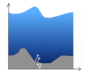
  $(x,y)$ plane, see figure 1. The domain is assumed to have the following description, for all time
  $t$,
$t$,
 \begin{equation} \varOmega(t) = \{ (x,y,z) \in \mathbb{R}^3 \, | \,z_b(x,y) < z < \eta(x,y,t) \}. \end{equation}
The boundaries of the domain are then defined by
 \begin{equation} \varGamma_s(t) = \{ (x,y,z) \in \mathbb{R}^3 \, | \,z = \eta(x,y,t) \}, \end{equation}
and
 \begin{equation} \varGamma_b(t) = \{ (x,y,z) \in \mathbb{R}^3 \, | \,z = z_b(x,y) - b(x,y,t)\}. \end{equation}
The function  $b$ is the source term, namely the normal displacement of the seabed. It can represent, for example, an earthquake or a landslide. It is assumed that this displacement starts at a time
  $t_0 > 0$, so that
  $b(x,y,0) = 0$.

Figure 1. The domain  $\varOmega (t)$: (a) for time
  $t=0$; (b) for time
  $t>0$. In panel (a), typical profiles for the temperature and the density at rest are drawn.
2.1. Euler equation in Eulerian coordinate
2.1.1. Equations in the volume
The unknowns are the fluid velocity  ${\boldsymbol U}$, its density
  $\rho$, its pressure
  $p$, its temperature
  $T$, its internal energy
  $e$ and its entropy
  $s$.
$s$.
For future reference, the equations are written for a viscous fluid with thermal dissipation. The stress tensor of a Newtonian fluid  $\boldsymbol{\mathsf{T}}$ has the form
 \begin{equation} \boldsymbol{\mathsf{T}} = ({-}p + \lambda \boldsymbol{\nabla} \boldsymbol{\cdot} {\boldsymbol U} ) \boldsymbol{\mathsf{I}} + 2 \mu \boldsymbol{\mathsf{D}}({\boldsymbol U}), \end{equation}
where  $\boldsymbol{\mathsf{D}}({\boldsymbol U})$ is defined by
  $\boldsymbol{\mathsf{D}}({\boldsymbol U}) = ( \frac {1}{2}(\partial _i {\boldsymbol U}^j + \partial _j {\boldsymbol U}^i) )_{i,j = x,y,z}$ and
  $\boldsymbol{\mathsf{I}}$ is the identity matrix in
  $\mathbb {R}^3$. The heat flux is denoted by
  ${\boldsymbol q}$ and is a function of
  $\rho$ and
  $T$.
$T$.
The conservation of mass, momentum and energy of a Newtonian fluid read, in the domain  $\varOmega (t)$,
 $$\begin{gather} \frac{\partial \rho}{\partial t} + \boldsymbol{\nabla}\boldsymbol{\cdot} (\rho {\boldsymbol U}) = 0, \end{gather}$$
 $$\begin{gather}
\frac{\partial}{\partial t} ( \rho {\boldsymbol U} ) +
\boldsymbol{\nabla}\boldsymbol{\cdot}( \rho {\boldsymbol
U}\otimes {\boldsymbol U}) + \boldsymbol{\nabla} p = \rho
{\boldsymbol g} + \boldsymbol{\nabla} (\lambda
\boldsymbol{\nabla} \boldsymbol{\cdot} {\boldsymbol U}) +
\boldsymbol{\nabla} \boldsymbol{\cdot} (2 \mu
\boldsymbol{\mathsf{D}}({\boldsymbol U})),
\end{gather}$$
$$\begin{gather}
\frac{\partial}{\partial t} ( \rho {\boldsymbol U} ) +
\boldsymbol{\nabla}\boldsymbol{\cdot}( \rho {\boldsymbol
U}\otimes {\boldsymbol U}) + \boldsymbol{\nabla} p = \rho
{\boldsymbol g} + \boldsymbol{\nabla} (\lambda
\boldsymbol{\nabla} \boldsymbol{\cdot} {\boldsymbol U}) +
\boldsymbol{\nabla} \boldsymbol{\cdot} (2 \mu
\boldsymbol{\mathsf{D}}({\boldsymbol U})),
\end{gather}$$
 $$\begin{gather}\hspace{-60pt}\frac{\partial }{\partial t} \left( \rho
\frac{|{\boldsymbol U}|^2}{2} + \rho e \right) +
\boldsymbol{\nabla} \boldsymbol{\cdot} \left( \left(\rho
\frac{|{\boldsymbol U}|^2}{2} + \rho e + p\right)
{\boldsymbol U} \right)\nonumber\\= \rho {\boldsymbol g}\boldsymbol{\cdot} {\boldsymbol U} + \boldsymbol{\nabla} \boldsymbol{\cdot} (\lambda {\boldsymbol U} \boldsymbol{\nabla} \boldsymbol{\cdot} {\boldsymbol U}) + \boldsymbol{\nabla} \boldsymbol{\cdot} (2 \mu \boldsymbol{\mathsf{D}}({\boldsymbol U}) \boldsymbol{\cdot} {\boldsymbol U}) - \boldsymbol{\nabla} \boldsymbol{\cdot} {\boldsymbol q} . \end{gather}$$
$$\begin{gather}\hspace{-60pt}\frac{\partial }{\partial t} \left( \rho
\frac{|{\boldsymbol U}|^2}{2} + \rho e \right) +
\boldsymbol{\nabla} \boldsymbol{\cdot} \left( \left(\rho
\frac{|{\boldsymbol U}|^2}{2} + \rho e + p\right)
{\boldsymbol U} \right)\nonumber\\= \rho {\boldsymbol g}\boldsymbol{\cdot} {\boldsymbol U} + \boldsymbol{\nabla} \boldsymbol{\cdot} (\lambda {\boldsymbol U} \boldsymbol{\nabla} \boldsymbol{\cdot} {\boldsymbol U}) + \boldsymbol{\nabla} \boldsymbol{\cdot} (2 \mu \boldsymbol{\mathsf{D}}({\boldsymbol U}) \boldsymbol{\cdot} {\boldsymbol U}) - \boldsymbol{\nabla} \boldsymbol{\cdot} {\boldsymbol q} . \end{gather}$$
The acceleration of gravity is  ${\boldsymbol g} = -g {\boldsymbol e}_3$ with
  $g>0$ and
  ${\boldsymbol e}_3$ is the unit vector in the vertical direction, oriented upwards.
To describe the acoustic waves, we derive an equation for the pressure. Among  $(\rho, e, T, p, s)$, only two variables are independent because of the Gibbs law and of the equation of state (Gill Reference Gill1982). When considering
  $\rho$ and
  $s$ as independent, it is natural to introduce the scalar functions
  $f_e$,
  $f_p$ and
  $f_T$ satisfying
 \begin{equation} e = f_e(\rho,s),\quad p = f_p(\rho,s),\quad T = f_T(\rho,s). \end{equation}
With the Gibbs law ( ${\partial f_e}/{\partial \rho } = {f_p}/{\rho ^2}$ and
  ${\partial f_e}/{\partial s} = f_T$), one has
 \begin{equation} \frac{\partial e}{\partial t} + {\boldsymbol U} \boldsymbol{\cdot} \boldsymbol{\nabla} e = \frac{f_p}{\rho^2} \left( \frac{\partial \rho}{\partial t} + {\boldsymbol U} \boldsymbol{\cdot} \boldsymbol{\nabla} \rho \right) +f_T \left( \frac{\partial s}{\partial t} + {\boldsymbol U} \boldsymbol{\cdot} \boldsymbol{\nabla} s \right). \end{equation}
Using (2.7)  $-{\boldsymbol U} \, \boldsymbol {\cdot }$ (2.6) and (2.9), one obtains as an intermediate step the evolution equation of the entropy,
 \begin{equation} \rho T \left(\frac{\partial s}{\partial t} + {\boldsymbol U} \boldsymbol{\cdot} \boldsymbol{\nabla} s\right) = \lambda (\boldsymbol{\nabla} \boldsymbol{\cdot} {\boldsymbol U})^2 + 2 \mu \boldsymbol{\mathsf{D}}({\boldsymbol U}) : \boldsymbol{\mathsf{D}}({\boldsymbol U}) - \boldsymbol{\nabla} \boldsymbol{\cdot} {\boldsymbol q}. \end{equation}
Now, since  $p=f_p(\rho,s)$, we have
 \begin{equation} \frac{\partial p}{\partial t} + {\boldsymbol U} \boldsymbol{\cdot} \boldsymbol{\nabla} p = \frac{\partial f_p}{\partial \rho} \left( \frac{\partial \rho}{\partial t} + {\boldsymbol U} \boldsymbol{\cdot} \boldsymbol{\nabla} \rho \right) + \frac{1}{T \rho} \frac{\partial f_p}{\partial s} \left( \frac{\partial s}{\partial t} + {\boldsymbol U} \boldsymbol{\cdot} \boldsymbol{\nabla} s \right), \end{equation}
hence using (2.5) and (2.10), one obtains
 \begin{align} \frac{\partial p}{\partial t} + {\boldsymbol U} \boldsymbol{\cdot} \boldsymbol{\nabla} p ={-} \frac{\partial f_p}{\partial \rho} ( \rho \boldsymbol{\nabla} \boldsymbol{\cdot} {\boldsymbol U} ) + \frac{1}{T \rho} \frac{\partial f_p}{\partial s} ( \lambda (\boldsymbol{\nabla} \boldsymbol{\cdot} {\boldsymbol U})^2 + 2 \mu \boldsymbol{\mathsf{D}}({\boldsymbol U}) : \boldsymbol{\mathsf{D}}({\boldsymbol U}) - \boldsymbol{\nabla} \boldsymbol{\cdot} {\boldsymbol q}). \end{align}
At this point, we use the common assumption that the viscous term and the thermal dissipation can be neglected compared with the advection term (see Lannes Reference Lannes2013, Chap. 1). With (2.10), we see that this is equivalent to assuming that the flow is isentropic. Moreover, from physical considerations, the function  $f_p$ must satisfy
  $\partial _{\rho } f_p (\rho,s) \geq 0$, hence we can introduce the speed of sound
  $c$ defined by
 \begin{equation} c^2 = \frac{\partial f_p}{\partial \rho} (\rho,s). \end{equation}
Equation (2.12) then reads
 \begin{equation} \frac{\partial p}{\partial t} + {\boldsymbol U} \boldsymbol{\cdot} \boldsymbol{\nabla} p + \rho c^2 \boldsymbol{\nabla} \boldsymbol{\cdot} {\boldsymbol U} = 0. \end{equation}
Equation (2.14) is used for the study of a compressible fluid in the isentropic case, see Gill (Reference Gill1982, Chap. 4). Note that the speed of sound  $c$ can also be viewed as a function of
  $p$ and
  $T$, and in that case, we have
 \begin{equation} c^2(p,T) = \frac{\partial f_p}{\partial \rho} ( f_{\rho}(p,T), f_s(p,T)). \end{equation}
In practice, we choose to work directly with the expression  $c=c(p,T)$ tabulated by International Association for the Properties of Water and Steam (2009). Note that here, the temperature intervenes as a side variable, because it is necessary to compute the speed of sound. However, we will see later that only the temperature profile of the state at rest is needed to close the system.
2.1.2. Boundary conditions
The following boundary conditions hold:
 $$\begin{gather} {\boldsymbol U} \boldsymbol{\cdot} {\boldsymbol n}_b = u_b = \partial_t b \quad \text{on } \varGamma_b, \end{gather}$$
 $$\begin{gather}p = p^a \quad \text{on } \varGamma_s. \end{gather}$$
The bottom boundary condition (2.16) is a non-penetration condition with a source term. It models the tsunami source as a displacement of the ocean bottom with velocity  $u_b$. We denote by
  ${\boldsymbol n}_b$ the unit vector normal to the bottom and oriented outwards. The second condition (2.17) is a dynamic condition, where we assume that the surface pressure is at equilibrium with a constant atmospheric pressure
  $p^a$. Note that the elevation
  $\eta$ is a solution of the following kinematic equation:
 \begin{equation} \dfrac{\partial \eta}{\partial t} + {\boldsymbol U} \boldsymbol{\cdot} \begin{pmatrix} \partial_x \eta \\ \partial_y \eta \\ -1 \end{pmatrix}= 0\quad \text{on} \ \varGamma_s(t). \end{equation}
2.1.3. Initial conditions and equilibrium state
It is assumed that the initial state corresponds to the rest state, meaning that  $\eta (x,y,0) = H$ with the elevation at rest
  $H$ being independent of space and
  $H > z_b(x,y)$; therefore,
 \begin{equation} \varOmega(0) = \{ (x,y,z) \in \mathbb{R}^3 \, | \,z_b(x,y) < z < H \}. \end{equation}
We choose the following initial conditions for the velocity, the temperature, the density and the pressure:
 $$\begin{gather} {\boldsymbol U}(x,y,z,0) = 0, \end{gather}$$
 $$\begin{gather}T(x,y,z,0) = T_0 (z),\quad \rho(x,y,z,0) = \rho_0 (z),\quad p(x,y,z,0) = p_0(z), \end{gather}$$
where  $T_0, \rho _0, p_0$ are functions defined on
  $(0,H)$ but because of the topography
  $z_b(x,y)$, the functions
  $T,\rho,p$ need not to be defined from
  $z=0$ for all
  $(x,y)$.
When the source term  $u_b$ vanishes, we have an equilibrium state around
  ${\boldsymbol U} \equiv 0$ if the functions
  $T_0, \rho _0, p_0$ satisfy
 \begin{equation} \boldsymbol{\nabla} p_0 = \rho_0 {\boldsymbol g}, \quad \rho_0 = f_{\rho}(p_0, T_0), \quad p_0(H) = p^a. \end{equation}
Hence, if  $T_0(z)$ is given, the system
 $$\begin{gather} \frac{{\rm d} p_0}{{\rm d} z} ={-}g f_{\rho}(p_0, T_0), \quad z \in (0, H), \end{gather}$$
 $$\begin{gather}p_0 = p^a, \quad z = H \end{gather}$$
can be solved to compute  $p_0$, and then
  $\rho _0$ is computed with
  $\rho _0 = f_{\rho }(p_0, T_0)$. Note that, in the forthcoming sections, the system (2.5), (2.6), (2.14) with boundary conditions (2.16), (2.17) and initial conditions (2.20), (2.21) will be linearized around the previously defined equilibrium state.
2.2. Lagrangian description
Although most of the works on free-surface flows are done in Eulerian coordinates, the Lagrangian formalism is sometimes preferred, see for example the paper by Nouguier, Chapron & Guérin (Reference Nouguier, Chapron and Guérin2015) and the references therein, or the work of Godlewski, Olazabal & Raviart (Reference Godlewski, Olazabal and Raviart1999) for a precise derivation of linear models. Here we choose the Lagrangian description to avoid any approximation on the shape of the domain when we linearize the equations. The usual approximation made on the surface for the linear models in Eulerian coordinates consists in evaluating the surface condition on pressure at a fixed height, rather than at the actual, time-dependant free surface. The kinematic boundary condition is also replaced by its linear approximation. For the derivation and justification of the approximation, see Lighthill (Reference Lighthill1978, Chap. 3).
Let  $\hat \varOmega$ be the domain of the ocean at a reference time, with its surface boundary
  $\hat \varGamma _s$ and bottom boundary
  $\hat \varGamma _b$. The reference time is chosen before the tsunami generation, so that the surface of the domain is horizontal. In fact, the following natural choice is made:
 \begin{equation} \hat \varOmega = \varOmega(0), \quad \hat \varGamma_s = \varGamma_s(0), \quad \hat \varGamma_b = \varGamma_b(0). \end{equation}
The position at the reference time of a fluid particle is denoted
 \begin{equation} {\boldsymbol \xi = (\xi^1, \xi^2, \xi^3) \in \hat \varOmega}. \end{equation}
At time  $t$, the fluid has moved, the domain is
  $\varOmega (t)$ and the new position of a fluid particle is
  ${\boldsymbol x} = (x(\boldsymbol \xi,t),y(\boldsymbol \xi,t),z(\boldsymbol \xi,t)) \in \varOmega (t)$. We denote by
  $\boldsymbol \phi$ the transformation from
  $\hat \varOmega$ to
  $\varOmega (t)$ that maps each particle from its reference position
  $\boldsymbol \xi$ to its position
  ${\boldsymbol x}$ at time
  $t$ (see figure 2):
 \begin{equation} \boldsymbol \phi : \begin{cases} \hat \varOmega \to \varOmega(t)\\ \boldsymbol \xi \mapsto {\boldsymbol x}(\boldsymbol \xi, t) \end{cases}. \end{equation}
Hence, one has  ${\boldsymbol x} = \boldsymbol \phi (\boldsymbol \xi,t)$. The transformation is assumed invertible, in particular, we do not consider the case of wave breaking. We also define the displacement of the fluid. For each fluid particle with initial position
  $\boldsymbol \xi$, its displacement is defined by
 \begin{equation} {\boldsymbol d}(\boldsymbol \xi,t) = \boldsymbol \phi(\boldsymbol \xi,t) - \boldsymbol \xi. \end{equation}
The gradient of  $\boldsymbol \phi$ with respect to
  $\boldsymbol \xi$ is denoted
  $\boldsymbol{\mathsf{F}}$,
 \begin{equation} \boldsymbol{\mathsf{F}} = \nabla_{\xi} \boldsymbol \phi, \end{equation}
and its determinant is denoted  $J$. Both
  $\boldsymbol{\mathsf{F}}$ and
  $J$ can be expressed as functions of the displacement,
 \begin{equation} \boldsymbol{\mathsf{F}} = \boldsymbol{\mathsf{I}} + \nabla_{\xi} {\boldsymbol d}, \quad J = \det \boldsymbol{\mathsf{F}}, \end{equation}
where  $\nabla _{\xi }$ is the gradient with respect to the coordinate system
  $\boldsymbol \xi$. For a function
  $X({\boldsymbol x}, t)$ defined on the domain
  $\varOmega (t)$, we introduce
  $\hat X(\boldsymbol \xi,t)$ defined on
  $\hat \varOmega$ by
 \begin{equation} \hat X(\boldsymbol \xi,t) = X(\boldsymbol \phi(\boldsymbol \xi,t),t). \end{equation}
Finally, note that the velocity  $\hat {\boldsymbol U}(\boldsymbol \xi,t) = {\boldsymbol U}(\boldsymbol \phi (\boldsymbol \xi,t),t)$ is the time derivative of the displacement
  ${\boldsymbol d}$,
 \begin{equation} \hat {\boldsymbol U} = \frac{\partial {\boldsymbol d}}{\partial t}. \end{equation}
With this change of coordinates, the system (2.5), (2.6), (2.14) is now defined in the time-independent reference domain  $\hat \varOmega$ and it reads
 $$\begin{gather} \frac{\partial \hat \rho}{\partial t} + \frac{\hat \rho}{|J|} \nabla_{\xi} \boldsymbol{\cdot}( |J| \boldsymbol{\mathsf{F}}^{{-}1} \hat {\boldsymbol U} ) = 0, \end{gather}$$
 $$\begin{gather}\hat \rho \frac{\partial \hat {\boldsymbol U}}{\partial t} + \boldsymbol{\mathsf{F}}^{{-}T} \nabla_{\xi} \hat p = \hat \rho {\boldsymbol g}, \end{gather}$$
 $$\begin{gather}\frac{\partial \hat p}{\partial t} + \frac{ \hat \rho \hat c^2 }{|J| } \nabla_{\xi} \boldsymbol{\cdot}( |J| \boldsymbol{\mathsf{F}}^{{-}1} \hat {\boldsymbol U} ) = 0. \end{gather}$$
The boundary conditions become
 $$\begin{gather} \hat {\boldsymbol U} \boldsymbol{\cdot} \hat{\boldsymbol{n}}_b = \hat u_b \quad \text{on } \hat \varGamma_b, \end{gather}$$
 $$\begin{gather}\hat p = p^a \quad \text{on } \hat \varGamma_s, \end{gather}$$
where  $\hat {\boldsymbol {n}}_b$ is a unit vector normal to
  $\hat \varGamma _b$ and pointing towards the exterior of the domain. The variables
  $\hat \rho, \hat p, \hat T$ satisfy the same equation of state,
 \begin{equation} \hat p = f_p(\hat \rho, \hat T), \end{equation}
and the speed of sound is a function of the new variables,  $\hat c = c(\hat \rho, \hat s)$.

Figure 2. The mapping  $\phi _t$ between the reference domain
  $\hat \varOmega = \varOmega (0)$ and the domain
  $\varOmega (t)$.
2.3. Linearization and wave equation
We assume that the source of the tsunami is a displacement of magnitude  $a$ at the seafloor occurring in an ocean at rest as described in § 2.1.3. In particular, for this rest state, there is no mean current and the temperature, pressure and density vary only vertically. The magnitude of the displacement is assumed small compared to the water height
  $H$. The ratio of the bottom displacement amplitude to the water height is denoted
  $\varepsilon = a/H \ll 1$, and the source term can be expressed as
 \begin{equation} \hat u_b = \varepsilon \hat u_{b,1} + {O}(\varepsilon^2). \end{equation}
The linearization of (2.33)–(2.35) around the rest state corresponds to the following asymptotic expansion:
 $$\begin{gather} {\boldsymbol d}(\boldsymbol \xi,t) = \varepsilon {\boldsymbol d}_1(\boldsymbol \xi,t) + {O}(\varepsilon^2), \end{gather}$$
 $$\begin{gather}\hat \rho(\boldsymbol \xi,t) = \hat \rho_0(\boldsymbol \xi) + \varepsilon \hat \rho_1(\boldsymbol \xi,t) + {O}(\varepsilon^2), \end{gather}$$
 $$\begin{gather}\hat p(\boldsymbol \xi,t) = \hat p_0(\boldsymbol \xi) + \varepsilon \hat p_1(\boldsymbol \xi,t) + {O}(\varepsilon^2). \end{gather}$$
Note that the displacement has no zero order term, because the reference configuration used to define the Lagrangian description is the state given by the initial conditions. It holds then that  ${\boldsymbol d}_0 = 0$,
  $\hat {\boldsymbol U}_0 = 0$ and
  $\hat \varOmega = \varOmega (0)$.
Remark In comparison with the linearization done by Auclair et al. (Reference Auclair, Debreu, Duval, Marchesiello, Blayo and Hilt2021), where the expansion of the density and the pressure is justified with the decomposition into hydrostatic and non-hydrostatic components, the asymptotic expansion (2.41)–(2.42) is obtained in a more straightforward way. Indeed, it only requires the assumption of a small perturbation.
From the expansion, one deduces the following Taylor expansions for the other functions:
 $$\begin{gather} \hat {\boldsymbol U} = \varepsilon \hat{\boldsymbol{U}}_1 + {O}(\varepsilon^2), \end{gather}$$
 $$\begin{gather}\boldsymbol{\mathsf{F}} = \boldsymbol{\mathsf{I}} + \varepsilon \nabla_{\xi} {\boldsymbol d}_1 + {O}(\varepsilon^2), \end{gather}$$
 $$\begin{gather}(\boldsymbol{\mathsf{F}})^{{-}1} = \boldsymbol{\mathsf{I}} - \varepsilon \nabla_{\xi} {\boldsymbol d}_1 + {O}(\varepsilon^2), \end{gather}$$
 $$\begin{gather}J = 1 + \varepsilon \nabla_{\xi} \boldsymbol{\cdot} {\boldsymbol d}_1 + {O}(\varepsilon^2). \end{gather}$$
Injecting these expressions in (2.33)–(2.35) yields the system
 $$\begin{gather} \frac{\partial}{\partial t} (\hat \rho_0 + \varepsilon \hat \rho_1 ) + \varepsilon \hat \rho_0 \nabla_{\xi} \boldsymbol{\cdot} \hat{\boldsymbol{U}}_1 = {O}(\varepsilon^2), \end{gather}$$
 $$\begin{gather}\varepsilon \hat \rho_0 \frac{\partial \hat{\boldsymbol{U}}_1}{\partial t} + (\boldsymbol{\mathsf{I}} - \varepsilon \nabla_{\xi} {\boldsymbol d}_1 )^{\rm T} \nabla_{\xi} \hat p_0 + \varepsilon \nabla_{\xi} \hat p_1 = (\hat \rho_0 + \varepsilon \hat \rho_1) {\boldsymbol g} + {O}(\varepsilon^2), \end{gather}$$
 $$\begin{gather}\frac{\partial}{\partial t} (\hat p_0 + \varepsilon \hat p_1) + \varepsilon \hat \rho_0 c^2(\hat p_0, \hat T_0) \nabla_{\xi} \boldsymbol{\cdot} \hat{\boldsymbol{U}}_1 = {O}(\varepsilon^2). \end{gather}$$
By separating the powers of  $\varepsilon$, we obtain two systems: a limit system when
  $\varepsilon \to 0$ and a system for the first-order corrections. Since the limit system corresponds to the initial conditions described in § 2.1.3, the model reduces to the first-order system.
2.3.1. First-order system: a wave-like equation for the velocity
The system for the correction terms reads in  $\hat \varOmega$,
 $$\begin{gather} \hat \rho_0 \frac{\partial \hat{\boldsymbol{U}}_1}{\partial t} + \nabla_{\xi} \hat p_1 - (\nabla_{\xi} {\boldsymbol d}_1)^{\rm T} \nabla_{\xi} \hat p_0 = \hat \rho_1 {\boldsymbol g}, \end{gather}$$
 $$\begin{gather}\frac{\partial \hat \rho_1}{\partial t} + \hat \rho_0 \nabla_{\xi} \boldsymbol{\cdot} \hat{\boldsymbol{U}}_1 = 0, \end{gather}$$
 $$\begin{gather}\frac{\partial \hat p_1}{\partial t} + \hat \rho_0 \hat c_0^2 \ \nabla_{\xi} \boldsymbol{\cdot} \hat{\boldsymbol{U}}_1 = 0, \end{gather}$$
with the boundary conditions
 $$\begin{gather} \hat{\boldsymbol{U}}_1 \boldsymbol{\cdot} \hat{\boldsymbol{n}}_b = \hat u_{b,1} \quad \text{on} \hat \varGamma_b, \end{gather}$$
 $$\begin{gather}\hat p_1 = 0 \quad \text{on } \hat \varGamma_s. \end{gather}$$
In this system, the speed of sound is evaluated at the limit – or background – pressure and temperature,  $\hat c_0 = c(\hat p_0, \hat T_0)$. In particular,
  $\hat c_0$ can be written as a function of depth. With an adapted temperature profile, it is then possible to recover the typical speed of sound profile creating the SOFAR channel.
The pressure  $\hat p_1$ and density
  $\hat \rho _1$ can be eliminated in (2.50) thanks to the other equations: differentiating in time (2.50) and replacing
  $\hat \rho _1$ and
  $\hat p_1$ with (2.51), (2.52), we obtain a second-order equation for
  $\hat {\boldsymbol {U}}_1$,
 \begin{equation} \hat \rho_0 \frac{\partial^2 \hat{\boldsymbol{U}}_1}{\partial t^2} - \nabla_{\xi} (\hat \rho_0 \hat c_0^2 \nabla_{\xi} \boldsymbol{\cdot} \hat{\boldsymbol{U}}_1) - (\nabla_{\xi} \hat{\boldsymbol{U}}_1)^{\rm T} \hat \rho_0 {\boldsymbol g} + \hat \rho_0 \nabla_{\xi} \boldsymbol{\cdot} \hat{\boldsymbol{U}}_1 \ {\boldsymbol g} = 0 \ \text{ in } \hat{\varOmega} . \end{equation}
Using (2.52), the surface boundary condition (2.54) is formulated for  $\hat {\boldsymbol {U}}_1$, hence the two boundary conditions for the wave-like equation (2.55) are
 $$\begin{gather} \hat{\boldsymbol{U}}_1 \boldsymbol{\cdot} \hat{\boldsymbol{n}}_b = \hat u_{b,1} \quad \text{on } \hat \varGamma_b, \end{gather}$$
 $$\begin{gather}\nabla_{\xi} \boldsymbol{\cdot} \hat{\boldsymbol{U}}_1 = 0 \quad \text{on }\hat \varGamma_s. \end{gather}$$
The wave-like equation (2.55) is completed with vanishing initial condition for  $\hat {\boldsymbol {U}}_1 (0)$ and
  $\partial _t \hat {\boldsymbol {U}}_1 (0)$. The system (2.55) includes both gravity and acoustic terms. This equation, which describes the velocity of a compressible, non-viscous fluid, in Lagrangian description, is called the Galbrun equation. It is used in helioseismology and in aeroacoustics (Legendre Reference Legendre2003; Maeder, Gabard & Marburg Reference Maeder, Gabard and Marburg2020; Hägg & Berggren Reference Hägg and Berggren2021). However, to our knowledge, this equation has never been used to describe the propagation of hydro-acoustic waves.
We show now that the system (2.55), (2.56), (2.57) is energy preserving. A model describing a physical system should either preserve or dissipate energy, and this property makes it also possible to write a stable numerical scheme. Here the energy equation is obtained by taking the scalar product of (2.55) with  $\partial _t \hat {\boldsymbol {U}}_1$ and integrating over the domain. After some computations (see Appendix A), we have
 \begin{equation} \frac{{\rm d}}{{\rm d}t} \mathcal{E} = \int_{\hat \varGamma_b} \hat \rho_0 ( c_0^2 \nabla_{\xi} \boldsymbol{\cdot} \hat{\boldsymbol{U}}_1 - \hat \rho_0 g \hat{\boldsymbol{U}}_1 \boldsymbol{\cdot} {\boldsymbol e}_3) \frac{\partial \hat u_{b,1}}{\partial t} \,\text{d} \sigma, \end{equation}
with the energy being the quadratic functional given by
 \begin{align} \mathcal{E} &= \int_{\hat \Omega} \rho_0 \frac{1}{2} \left| \frac{\partial \hat{\boldsymbol{U}}_1}{\partial t} \right|^2 \text{d} \boldsymbol \xi + \frac{1}{2} \int_{\hat \Omega} \hat \rho_0 \left( \hat c_0 \nabla_{\xi} \boldsymbol{\cdot} \hat{\boldsymbol{U}}_1 - \frac{g}{\hat c_0} \hat{\boldsymbol{U}}_1 \boldsymbol{\cdot} {\boldsymbol e}_3 \right)^2 \text{d} \boldsymbol \xi\nonumber\\ &\quad + \frac{1}{2} \int_{\hat \Omega} \hat \rho_0 N_b (\hat{\boldsymbol{U}}_1 \boldsymbol{\cdot} {\boldsymbol e}_3)^2 \,\text{d} \boldsymbol \xi + \frac{1}{2} \int_{\hat{\varGamma}_s} \hat \rho_0 g (\hat{\boldsymbol{U}}_1 \boldsymbol{\cdot} {\boldsymbol e}_3)^2 \,\text{d} \sigma. \end{align}
The scalar  $N_b$ is the squared Brunt–Väsisälä frequency, defined by
 \begin{equation} N_b(\xi^3) ={-} \left( \frac{g^2}{\hat c_0(\xi^3)^2} + g \frac{\hat \rho_0'(\xi^3)}{\hat \rho_0(\xi^3)}\right). \end{equation}
The Brunt–Väisälä frequency, or buoyancy frequency, is closely related to the internal waves that appear in a stratified medium (Gill Reference Gill1982, Chap. 6). In the ocean, the usual values of  $N_b$ are approximately
  $10^{-8} \ \text {rad}^2\ \text {s}^{-2}$ (King et al. Reference King, Stone, Zhang, Gerkema, Marder, Scott and Swinney2012).
The physical interpretation for the different terms in the energy is clearer when one writes the wave-like equation (2.55) in terms of the displacement  ${\boldsymbol d}_1$ instead of the velocity
  $\hat {\boldsymbol {U}}_1$. Using
  $\partial _t {\boldsymbol d}_1=\hat {\boldsymbol {U}}_1$ and integrating (2.55) once in time with the vanishing initial conditions for the displacement, one obtains
 \begin{equation} \hat \rho_0 \frac{\partial^2 {\boldsymbol d}_1}{\partial t^2} - \nabla_{\xi} ( \hat \rho_0 \hat c_0^2 \nabla_{\xi} \boldsymbol{\cdot} {\boldsymbol d}_1 ) - (\nabla_{\xi} {\boldsymbol d}_1)^{\rm T} \hat \rho_0 {\boldsymbol g} + \hat \rho_0 \nabla_{\xi} \boldsymbol{\cdot} {\boldsymbol d}_1 {\boldsymbol g} = 0 \quad \text{in } \hat{\varOmega} . \end{equation}
The exact same steps of Appendix A, with  ${\boldsymbol d}_1$ instead of
  $\hat {\boldsymbol {U}}_1$, yield the energy equation
 \begin{equation} \frac{{\rm d}}{{\rm d}t} \mathcal{E}_d = \int_{\hat \varGamma_b} \hat \rho_0 ( c_0^2 \nabla_{\xi} \boldsymbol{\cdot} {\boldsymbol d}_1 - \hat \rho_0 g {\boldsymbol d}_1 \boldsymbol{\cdot} {\boldsymbol e}_3) \hat u_{b,1} \,\text{d} \sigma, \end{equation}
with the energy
 \begin{align} \mathcal{E}_d &= \int_{\hat \Omega} \hat \rho_0 \frac{1}{2} | \hat{\boldsymbol{U}}_1 |^2 \,\text{d} \boldsymbol \xi + \frac{1}{2} \int_{\hat \Omega} \hat \rho_0 \left( \hat c_0 \nabla_{\xi} \boldsymbol{\cdot} {\boldsymbol d}_1 - \frac{g}{\hat c_0} {\boldsymbol d}_1 \boldsymbol{\cdot} {\boldsymbol e}_3 \right)^2 \text{d} \boldsymbol \xi\nonumber\\ &\quad + \frac{1}{2} \int_{\hat \Omega} \hat \rho_0 N_b ({\boldsymbol d}_1 \boldsymbol{\cdot} {\boldsymbol e}_3)^2 \,\text{d} \boldsymbol \xi + \frac{1}{2} \int_{\hat{\varGamma}_s} \hat \rho_0 g ({\boldsymbol d}_1\boldsymbol{\cdot} {\boldsymbol e}_3)^2 \,\text{d} \sigma. \end{align}
The first term in (2.63) is the kinetic energy. We show that the second term of (2.63) corresponds to the acoustic energy. First, using (2.52) with the vanishing initial conditions yields  $\hat \rho _0 \hat c_0^2 \boldsymbol {\cdot } \nabla _{\xi } {\boldsymbol d}_1 = - \hat p_1$. We define then the acoustic pressure
 \begin{equation} p_a = \hat p_1 - \boldsymbol{\nabla} \hat p_0 \boldsymbol{\cdot} {\boldsymbol d}_1. \end{equation}
Indeed, in Lagrangian coordinates, the pressure perturbation  $\hat p_1$ has two contributions: the small variations in acoustic pressure and the background pressure being evaluated at a new position. With the definition of
  $p_a$ and (2.24), it holds that for the second term of (2.63),
 \begin{equation} \frac{1}{2} \int_{\hat \Omega} \hat \rho_0 \left( \hat c_0 \nabla_{\xi} \boldsymbol{\cdot} {\boldsymbol d}_1 - \frac{g}{\hat c_0} {\boldsymbol d}_1 \boldsymbol{\cdot} {\boldsymbol e}_3 \right)^2 \text{d} \boldsymbol \xi =\frac{1}{2} \int_{\hat \Omega} \frac{p_a^2}{\hat \rho_0 \hat c_0^2} \,\text{d} \boldsymbol \xi, \end{equation}
which is the usual expression for the acoustic energy (Lighthill Reference Lighthill1978). The last term of (2.63) is the potential energy associated with the surface waves. Finally, the third term of (2.63) is the potential energy associated with the internal gravity waves (Lighthill Reference Lighthill1978), under the condition
 \begin{equation} N_b > 0. \end{equation}
When  $N_b$ is positive, it is denoted
  $N_b=N^2$, where
  $N$ is the buoyancy frequency. The sign of
  $N_b$ depends on the choice of the state at equilibrium:
  $\hat \rho _0'={\rm d}\hat \rho _0/{\rm d}z$ has to be negative and satisfy
 \begin{equation} \frac{|\hat \rho_0'|}{\hat \rho_0} > \frac{g}{\hat c_0^2}. \end{equation}
With the term in  $g^2 / \hat c_0^2$, we see that the compressibility tends to take the fluid away from its equilibrium. The stratification of the fluid must be strong enough to counter this effect and keep the system stable (see the discussion in Gill Reference Gill1982, Chap. 3). As a consequence, if one wants the model to preserve the energy of the system, the background density should not be assumed homogeneous. In the following, we assume that the fluid has a stable stratification, namely that the function
  $N_b$ is assumed always positive. We will use the notation
  $N^2$ in the rest of this paper.
Remark According to the equation of state (when the salinity is neglected)  $\rho = f_{\rho }(p,T)$, the background density varies because of the variations in temperature and in pressure. The temperature profile can be chosen homogeneous, but the effect of gravity – see (2.24) – prevents the pressure to be independent of depth. Hence in a model with gravity, the fluid is always stratified with the density increasing with depth.

3. Derivation of simplified models
To compare with existing models, we present several simplifications of our model. We first show that in the barotropic case, the system (2.55)–(2.57) is equivalent to the first-order scalar equation of Longuet-Higgins (Reference Longuet-Higgins1950). Our model also reduces to well-known models in the acoustic and incompressible asymptotic regimes, as demonstrated below. Further numerical implementations of our model will make it possible to quantify the impact of assumptions made in more simple models, in particular in the case of acoustic-gravity wave generation by earthquakes or landslides in the ocean.
3.1. The barotropic case
We consider the barotropic case, which is a very common assumption for the study of hydro-acoustic waves (see for example Longuet-Higgins Reference Longuet-Higgins1950, Stiassnie Reference Stiassnie2010). For a barotropic fluid, the pressure is a function of the density only,
 \begin{equation} f_p(\rho,s) = f_p(\rho) = p. \end{equation}
Then, using (2.22) and the definition of the speed of sound,
 \begin{equation} \hat p_0' = \hat \rho_0' \frac{{\rm d} f_p}{{\rm d} \rho} (\hat \rho_0) \ \Rightarrow\ - \hat \rho_0 g = \hat \rho_0' \hat c_0^2, \end{equation}
meaning that the Brunt–Väisälä frequency vanishes,  $N^2=0$. This corresponds to the case where the density is stratified because of the variation of pressure only. To use this equality, we divide (2.55) by
  $\hat \rho _0$,
 \begin{equation} \frac{\partial^2 \hat{\boldsymbol{U}}_1}{\partial t^2} - \nabla_{\xi} (\hat c_0^2 \nabla_{\xi} \boldsymbol{\cdot} \hat{\boldsymbol{U}}_1) - \left( \frac{\hat \rho_0'}{\rho_0} \hat c_0^2 + g \right) \nabla_{\xi} \boldsymbol{\cdot} \hat{\boldsymbol{U}}_1 {\boldsymbol e}_3 + \nabla_{\xi} (\hat{\boldsymbol{U}}_1 \boldsymbol{\cdot} {\boldsymbol e}_3) g = 0, \end{equation}
and when (3.2) holds, the (3.3) can be simplified and reads
 \begin{equation} \frac{\partial^2 \hat{\boldsymbol{U}}_1}{\partial t^2} - \nabla_{\xi} ( \hat c_0^2 \nabla_{\xi} \boldsymbol{\cdot} \hat{\boldsymbol{U}}_1 ) + \nabla_{\xi} (\hat{\boldsymbol{U}}_1 \boldsymbol{\cdot} {\boldsymbol e}_3) g = 0. \end{equation}
Taking the curl of (3.4) yields
 \begin{equation} \frac{\partial^2 \nabla_{\xi} \times \hat{\boldsymbol{U}}_1}{\partial t^2} = 0 \quad \text{in } \hat{\varOmega}. \end{equation}
With the vanishing initial conditions, we obtain that the velocity of a barotropic fluid is irrotational. This is a well-known result, since the fluid is also inviscid and subject to a potential force only (Guyon Reference Guyon2001, Chap. 7). By the Helmholtz decomposition theorem (Girault & Raviart Reference Girault and Raviart1986), the fluid velocity is written as the gradient of a potential  $\psi$ defined up to a constant. The expression
  $\hat {\boldsymbol U}_1 = \nabla _{\xi } \psi$ is used in (3.4) to obtain
 \begin{equation} \nabla_{\xi} \left( \frac{\partial^2 \psi}{\partial t^2} - \hat c_0^2 \Delta_{\xi} \psi + g \frac{\partial \psi}{\partial \xi^3} \right) = 0 . \end{equation}
The potential  $\psi$ being defined up to a constant, it can always be sought as the solution of
 \begin{equation} \frac{\partial^2 \psi}{\partial t^2} - \hat c_0^2 \Delta_{\xi} \psi + g \frac{\partial \psi}{\partial \xi^3} = 0 . \end{equation}
Equation (3.7) is multiplied by  $\hat \rho _0 / \hat c_0^2$, and we use
  $g/\hat c_0^2 = - \hat \rho _0'/\hat \rho _0$,
 \begin{equation} \frac{\hat \rho_0}{\hat c_0^2} \frac{\partial^2 \psi}{\partial t^2} - \hat \rho_0 \Delta_{\xi} \psi - \hat \rho_0' \frac{\partial \psi}{\partial \xi^3} = 0. \end{equation}
Additionally, since  $\hat \rho _0$ depends only on
  $\xi ^3$, the two last terms can be rewritten,
 \begin{equation} \frac{\hat \rho_0}{\hat c_0^2} \frac{\partial^2 \psi}{\partial t^2} - \nabla_{\xi} \boldsymbol{\cdot} ( \hat \rho_0 \nabla_{\xi} \psi ) = 0. \end{equation}
Hence,  $\psi$ satisfies a wave equation. The boundary conditions are then deduced from (2.56) and (2.57),
 $$\begin{gather} \nabla_{\xi} \psi \boldsymbol{\cdot} \hat{\boldsymbol{n}}_b = \hat u_{b,1} \quad \text{on } \hat \varGamma_b, \end{gather}$$
 $$\begin{gather}\hat c_0^2 \Delta_{\xi} \psi = \frac{\partial^2 \psi}{\partial t^2} + g \frac{\partial \psi}{\partial \xi^3} = 0 \quad \text{on }\hat \varGamma_s. \end{gather}$$
The system (3.7), (3.10), (3.11) is the first-order system obtained by Longuet-Higgins (Reference Longuet-Higgins1950). In Longuet-Higgins (Reference Longuet-Higgins1950), the derivation is quite different since the irrotationality assumption is made independently from the fact that the fluid is barotropic, and the boundary conditions are obtained from a linearized surface condition. The linearization made by Longuet-Higgins (Reference Longuet-Higgins1950) gives exactly the same result as the linearization strategy we have presented.
We show that the system (3.9)–(3.11) is energy preserving. Equation (3.9) is multiplied by  $\partial _t \psi$ and integrated by parts,
 \begin{align} &\int_{\hat \Omega} \frac{\hat \rho_0}{\hat c_0^2} \frac{\partial \psi}{\partial t} \frac{\partial^2 \psi}{\partial t^2} \,\text{d} \boldsymbol \xi + \int_{\hat \Omega} \hat \rho_0 \boldsymbol{\nabla} \left(\frac{\partial \psi}{\partial t} \right) \boldsymbol{\cdot} \boldsymbol{\nabla} \psi \,\text{d} \boldsymbol \xi\nonumber\\ &\quad - \int_{\hat \varGamma_s} \hat \rho_0 \frac{\partial \psi}{\partial t} \boldsymbol{\nabla} \psi \boldsymbol{\cdot} {\boldsymbol e}_3 \,\text{d} \sigma + \int_{\hat \varGamma_b} \hat \rho_0 \frac{\partial \psi}{\partial t} \boldsymbol{\nabla} \psi \boldsymbol{\cdot} {\boldsymbol n}_b \,\text{d} \sigma = 0. \end{align}
With the boundary conditions (3.10)–(3.11) and after simplifications,
 \begin{equation} \frac{{\rm d}}{{\rm d}t} \mathcal{E}_{bar} ={-} \int_{\hat{\varGamma}_b} \hat \rho_0 \frac{\partial \psi}{\partial t} \hat u_{b,1} \,\text{d} \sigma, \end{equation}
where the energy  $\mathcal {E}_{bar}$ is defined by
 \begin{equation} \mathcal{E}_{bar} = \frac{1}{2}\int_{\hat \Omega} \frac{\hat \rho_0}{\hat c_0^2} \left( \frac{\partial \psi}{\partial t} \right)^2 \text{d} \boldsymbol \xi + \frac{1}{2} \int_{\hat \Omega} \hat \rho_0 |\boldsymbol{\nabla} \psi |^2 \,\text{d} \boldsymbol \xi + \frac{1}{2} \int_{\hat{\varGamma}_s} \frac{\hat \rho_0}{g} \left(\frac{\partial \psi}{\partial t}\right)^2 \text{d} \boldsymbol \xi . \end{equation}
The first term of (3.14) is the acoustic energy. Indeed, with (2.14) and (3.2), one can show that the acoustic pressure  $p_a$ and the potential
  $\psi$ satisfy the usual relation
  $p_a = - \hat \rho _0 \partial _t \psi$ (Lighthill Reference Lighthill1978, Chap.3). The second term of (3.14) is the kinetic energy. Finally, with (3.11), one sees that the third term of (3.14) is the potential energy of the surface waves. To obtain the energy equation for the barotropic system (3.9), it is necessary to use the background density
  $\hat \rho _0$ even if it does not appear in (3.9). The correct manipulation for writing the energy equation was found by comparison with the general case described by (2.55).
Finally, note that when assuming a homogeneous density in the (3.9), the system (3.9)–(3.11) reduce to
 $$\begin{gather} \frac{\partial^2 \psi}{\partial t^2} - \hat c_0^2 \Delta \psi = 0 \quad \text{in } \hat \varOmega, \end{gather}$$
 $$\begin{gather}\nabla_{\xi} \psi \boldsymbol{\cdot} \hat{\boldsymbol{n}}_b = \hat u_{b,1} \quad \text{on } \hat \varGamma_b, \end{gather}$$
 $$\begin{gather}\frac{\partial^2 \psi}{\partial t^2} + g \frac{\partial \psi}{\partial \xi^3} = 0 \quad \text{on }\hat \varGamma_s, \end{gather}$$
and the energy (3.14) is not modified by this assumption. However, assuming a homogeneous density is not compatible with the derivation of the system (3.9)–(3.11), which relies on the equality  $g/\hat c_0^2 = - \hat \rho _0'/\hat \rho _0$. The model (3.15)–(3.17) can be understood as a barotropic model with the additional assumption that both
  $- \hat \rho _0'/\hat \rho _0$ and
  $g/\hat c_0^2$ are neglected inside the domain.
3.2. Two asymptotic regimes of the system
In this section, we write the limit models for two asymptotic regimes of the system (2.55)–(2.57). We consider the incompressible regime, where the acoustic waves are neglected, and the acoustic regime, where the effect of gravity is neglected. The wave equation (2.55) is written in non-dimensional form, and we show that it depends on a small non-dimensional parameter. A simplified model is then obtained by passing formally to the limit when the small parameter vanishes. By making the appropriate choice for the time scale, we obtain first an incompressible approximation, then an acoustic approximation.
3.2.1. Non-dimensional equation
We introduce the following characteristic scales for the system: a time  $\tau$, a horizontal scale
  $L$, a vertical scale
  $H$, a density
  $\bar \rho$ and a fluid velocity
  $U$. Since the speed of sound is not assumed constant, we denote by
  $C$ its characteristic magnitude. Finally, the surface waves velocity is of the order of
  $\sqrt {gH}$ (Constantin Reference Constantin2009). We focus on a non-shallow water formulation, hence we take
  $L = H$. For a shallow water version of the equation, one would choose
  $H \ll L$.
Two dimensionless numbers are introduced: the Froude number and the Mach number, respectively defined by
 \begin{equation} \text{Fr} = \frac{U}{\sqrt{gH}}, \quad \text{Ma} = \frac{U}{C}. \end{equation}
To fix the idea, we choose the following numerical values respectively for the speed of sound, the fluid velocity and the surface waves velocity:  $C \sim 1480\ {\rm m\ s}^{-1}$,
  $U \sim 1 \ {\rm m\ s}^{-1}$ and
  $\sqrt {gH} \sim 100 \text { m s}^{-1}$. The dimensionless numbers are then
 \begin{equation} \text{Fr} = 0.01, \quad \text{Ma} = 6.10^{{-}4}. \end{equation}
The characteristic scale for time will be fixed later, as it will depend on the regime we want to study. The variables are put in non-dimensional form and the dimensionless variables are denoted with a  $\tilde {\cdot }$, except for the space and time variable for the sake of conciseness. The adimensionned domain is denoted by
  $\tilde \varOmega$ and its surface and bottom boundary are respectively
  $\tilde \varGamma _s$ and
  $\tilde \varGamma _b$. The non-dimensional system reads, after simplification by the factor
  $\bar \rho U$,
 \begin{equation} \frac{\tilde \rho_0 }{\tau^2} \frac{\partial^2 \tilde{\boldsymbol{U}}_1}{\partial t^2} - \frac{C^2}{L^2} \nabla_{\xi} (\tilde \rho_0 \tilde c_0^2 \nabla_{\xi} \boldsymbol{\cdot} \tilde{\boldsymbol{U}}_1) + \frac{g}{L} \tilde \rho_0 (\nabla_{\xi} ( \tilde{\boldsymbol{U}}_1 \boldsymbol{\cdot} {\boldsymbol e}_3 ) - \nabla_{\xi} \boldsymbol{\cdot} \tilde{\boldsymbol{U}}_1 {\boldsymbol e}_3 ) = 0, \end{equation}
with the boundary conditions
 $$\begin{gather} \tilde{\boldsymbol{U}}_1 \boldsymbol{\cdot} \widetilde{{\boldsymbol n}_b} = \tilde u_{b,1} \quad \text{on } \tilde \varGamma_b, \end{gather}$$
 $$\begin{gather}\nabla_{\xi} \boldsymbol{\cdot} \tilde{\boldsymbol{U}}_1 = 0 \quad \text{on } \tilde \varGamma_s, \end{gather}$$
where  $\tilde u_{b,1}$ is a dimensionless source term.
3.2.2. Incompressible limit
We show that in the incompressible regime, our model is an extension of the classical free-surface Poisson equation to the case of a variable background density.
To study the incompressible limit, the characteristic time  $\tau$ is chosen to follow the surface waves, which are much slower than the acoustic waves. We take
  $L/\tau = \sqrt {gH}$. Equation (3.20) becomes
 \begin{equation} \tilde \rho_0 \frac{\partial^2 \tilde{\boldsymbol{U}}_1}{\partial t^2} - \frac{\text{Fr}}{\text{Ma}} \nabla_{\xi} ( \tilde \rho_0 \tilde c_0^2 \nabla_{\xi} \boldsymbol{\cdot} \tilde{\boldsymbol{U}}_1) + \tilde \rho_0 ( \nabla_{\xi} ( \tilde{\boldsymbol{U}}_1 \boldsymbol{\cdot} {\boldsymbol e}_3 ) - \nabla_{\xi} \boldsymbol{\cdot} \tilde{\boldsymbol{U}}_1 {\boldsymbol e}_3 )= 0. \end{equation}
The small parameter  $\delta = \text {Ma}/\text {Fr} \sim 6.10^{-2}$ is introduced in the equation,
 \begin{equation} \tilde \rho_0 \frac{\partial^2 \tilde{\boldsymbol{U}}_1}{\partial t^2} - \frac{1}{\delta^2} \nabla_{\xi} ( \tilde \rho_0 \tilde c_0^2 \nabla_{\xi} \boldsymbol{\cdot} \tilde{\boldsymbol{U}}_1) + \tilde \rho_0 ( \nabla_{\xi} ( \tilde{\boldsymbol{U}}_1 \boldsymbol{\cdot} {\boldsymbol e}_3 ) - \nabla_{\xi} \boldsymbol{\cdot} \tilde{\boldsymbol{U}}_1 {\boldsymbol e}_3 ) = 0, \end{equation}
and the goal is now to calculate the limit of (3.24) when  $\delta$ goes to zero. We make the following ansatz for
  $\tilde {\boldsymbol {U}}_1$:
 \begin{equation} \tilde{\boldsymbol{U}}_1 =\tilde{\boldsymbol{U}}_{1, 0} +\delta^2 \tilde{\boldsymbol{U}}_{1, 2}+ {O}(\delta^3), \end{equation}
where  $\tilde {\boldsymbol {U}}_{1, 0}$,
  $\tilde {\boldsymbol {U}}_{1, 1}$ and
  $\tilde {\boldsymbol {U}}_{1, 2}$ are independent of
  $\delta$. Since (3.24) has only even powers of
  $\delta$, the term
  $\tilde {\boldsymbol {U}}_{1, 1}$ is equal to zero. Replacing
  $\tilde {\boldsymbol {U}}_1$ by its ansatz in the wave equation (3.24) and separating the powers of
  $\delta$ yields an equation for each term of the asymptotic development of
  $\tilde {\boldsymbol {U}}_1$.
The equation obtained with the terms in  $\delta ^{-2}$ reads
 \begin{equation} \nabla_{\xi} (\tilde \rho_0 \tilde c_0^2 \nabla_{\xi} \boldsymbol{\cdot} \tilde{\boldsymbol{U}}_{1, 0}) = 0, \end{equation}
and the equation obtained with the terms in  $\delta ^0$ reads
 \begin{equation} \tilde \rho_0 \frac{\partial^2 \tilde{\boldsymbol{U}}_{1, 0}}{\partial t^2} - \nabla_{\xi} ( \tilde \rho_0 \tilde c_0^2 \nabla_{\xi} \boldsymbol{\cdot} \tilde{\boldsymbol{U}}_{1, 2}) + \tilde \rho_0 ( \nabla_{\xi} ( \tilde{\boldsymbol{U}}_{1, 0} \boldsymbol{\cdot} {\boldsymbol e}_3 ) - \nabla_{\xi} \boldsymbol{\cdot} \tilde{\boldsymbol{U}}_{1, 0}\, {\boldsymbol e}_3 ) = 0 .\end{equation}
With the terms in  $\delta ^0$ of the boundary conditions, we have
 $$\begin{gather} \nabla_{\xi} \boldsymbol{\cdot} \tilde{\boldsymbol{U}}_{1, 0} = 0 \quad \text{on } \tilde \varGamma_s, \end{gather}$$
 $$\begin{gather}\tilde{\boldsymbol{U}}_{1, 0} \boldsymbol{\cdot} \widetilde{{\boldsymbol n}}_b = \tilde u_{b,1} \quad \text{on } \tilde \varGamma_b. \end{gather}$$
Additionally, the terms in  $\delta ^2$ of the boundary conditions read
 $$\begin{gather} \nabla_{\xi} \boldsymbol{\cdot} \tilde{\boldsymbol{U}}_{1, 2} = 0 \quad \text{on } \tilde \varGamma_s, \end{gather}$$
 $$\begin{gather}\tilde{\boldsymbol{U}}_{1, 2} \boldsymbol{\cdot} \widetilde{{\boldsymbol n}}_b = 0 \quad \text{on } \tilde \varGamma_b. \end{gather}$$
 We show now that the limit model represents an incompressible flow. The Helmoltz decomposition of  $\tilde {\boldsymbol {U}}_{1, 0}$ reads
 \begin{equation} \tilde{\boldsymbol{U}}_{1, 0} = \nabla_{\xi} \varphi_{1,0} + \nabla_{\xi} \times \boldsymbol \psi_{1,0}, \end{equation}
where  $\varphi _{1,0}$ vanishes on
  $\tilde \varGamma _s$ and
  $\tilde \varGamma _b$. Injecting the decomposition of
  $\tilde {\boldsymbol {U}}_{1, 0}$ in (3.26) yields
 \begin{equation} \nabla_{\xi}( \tilde \rho_0 \tilde c_0^2 \ \Delta_{\xi} \varphi_{1,0} ) = 0, \end{equation}
hence the term inside the gradient is constant in space. Since the velocity  $\tilde {\boldsymbol {U}}_{1, 0}$ is equal to zero at infinity, we obtain that
  $\Delta _{\xi } \varphi _{1,0} = 0$ in
  $\tilde \varOmega$ (the quantity
  $\tilde \rho _0 \tilde c_0$ being always strictly positive). With the vanishing boundary conditions for
  $\varphi _{1,0}$, we obtain that
  $\varphi _{1,0}$ is equal to zero everywhere in
  $\tilde \varOmega$. Then, taking the divergence of
  $\tilde {\boldsymbol {U}}_{1, 0}$ yields
 \begin{equation} \nabla_{\xi} \boldsymbol{\cdot} \tilde{\boldsymbol{U}}_{1, 0} = \nabla_{\xi} \boldsymbol{\cdot} (\nabla_{\xi} \times \boldsymbol \psi_{1,0}) = 0, \end{equation}
hence  $\tilde {\boldsymbol {U}}_{1, 0}$ is divergence-free.
Now, using the property  $\boldsymbol {\nabla } \boldsymbol {\cdot } \tilde {\boldsymbol {U}}_{1, 0}$ in (3.27) and rearranging some terms, we obtain
 \begin{equation} \tilde \rho_0 \frac{\partial^2 \tilde{\boldsymbol{U}}_{1, 0}}{\partial t^2} - \nabla_{\xi} (\tilde \rho_0 \tilde c_0^2 \nabla_{\xi} \boldsymbol{\cdot} \tilde{\boldsymbol{U}}_{1, 2}) + \nabla_{\xi} ( \tilde \rho_0 \tilde{\boldsymbol{U}}_{1, 0} \boldsymbol{\cdot} {\boldsymbol e}_3 ) - \tilde \rho_0 ' ( \tilde{\boldsymbol{U}}_{1, 0} \boldsymbol{\cdot} {\boldsymbol e}_3 ) {\boldsymbol e}_3 = 0. \end{equation}
Taking the curl of this equation yields
 \begin{equation} \nabla_{\xi} \times \left( \tilde \rho_0 \frac{\partial^2 \tilde{\boldsymbol{U}}_{1, 0}}{\partial t^2} - \tilde \rho_0 ' ( \tilde{\boldsymbol{U}}_{1, 0} \boldsymbol{\cdot} {\boldsymbol e}_3 ) {\boldsymbol e}_3\right) = 0 . \end{equation}
This means that these terms can be expressed as the gradient of a potential function defined up to a constant and denoted  $- \tilde \varphi _0$,
 \begin{equation} \tilde \rho_0 \frac{\partial^2 \tilde{\boldsymbol{U}}_{1, 0}}{\partial t^2} - \tilde \rho_0 ' ( \tilde{\boldsymbol{U}}_{1, 0} \boldsymbol{\cdot} {\boldsymbol e}_3 ) {\boldsymbol e}_3 ={-} \nabla_{\xi} \tilde \varphi_0. \end{equation}
The new function  $\tilde \varphi _0$ can be understood as the Lagrange multiplier for the incompressibility constraint. However, one must be cautious that
  $\tilde \varphi _0$ is not similar to a pressure in this case, and rather plays the role of a velocity potential, as we will see later in the case of homogeneous density. The function
  $\tilde \varphi _0$ can be expressed differently. By using the definition (3.37) in (3.35), we have
 \begin{equation} \nabla_{\xi} ( - \tilde \varphi_0 - \tilde \rho_0 \tilde c_0^2 \nabla_{\xi} \boldsymbol{\cdot} \tilde{\boldsymbol{U}}_{1, 2} + \tilde \rho_0 \tilde{\boldsymbol{U}}_{1, 0} \boldsymbol{\cdot} {\boldsymbol e}_3 ) = 0, \end{equation}
and since the potential  $\tilde \varphi _0$ is defined up to a constant, it can be chosen such that, in
  $\hat \varOmega$, we have
 \begin{equation} \tilde \varphi_0 ={-} \tilde \rho_0 \tilde c_0^2 \nabla_{\xi} \boldsymbol{\cdot} \tilde{\boldsymbol{U}}_{1, 2} + \tilde \rho_0 \tilde{\boldsymbol{U}}_{1, 0} \boldsymbol{\cdot} {\boldsymbol e}_3. \end{equation}
We deduce from this equality and (3.30) the boundary condition
 \begin{equation} \tilde \varphi_0 = \tilde \rho_0 \tilde{\boldsymbol{U}}_{1, 0} \boldsymbol{\cdot} {\boldsymbol e}_3 \quad \text{on } \tilde \varGamma_s. \end{equation}
To recover a dimensional system, the terms are multiplied by their corresponding characteristic scales, and  $\hat \varphi _0 = \bar \rho U \tilde \varphi _0$ is defined. The limit solution
  $\hat {\boldsymbol {U}}_{1, 0} = U \tilde {\boldsymbol {U}}_{1, 0}$ satisfies
 $$\begin{gather} \hat \rho_0 \frac{\partial^2 \hat {\bf U}_{1,0}}{\partial t^2} - g \hat \rho_0' (\hat{\boldsymbol{U}}_{1, 0} \boldsymbol{\cdot} {\boldsymbol e}_3) {\boldsymbol e}_3 + g \nabla_{\xi} \hat \varphi_0 = 0 \quad \text{in } \hat \Omega, \end{gather}$$
 $$\begin{gather}\nabla_{\xi} \boldsymbol{\cdot} \hat {\bf U}_{1,0} = 0 \quad \text{ in } \hat \Omega, \end{gather}$$
with the boundary conditions
 $$\begin{gather} \hat{\boldsymbol{U}}_{1, 0} \boldsymbol{\cdot} \hat{\boldsymbol{n}}_b = \hat u_{b,1} \quad \text{on } \hat\varGamma_b, \end{gather}$$
 $$\begin{gather}\nabla_{\xi} \boldsymbol{\cdot} \hat{\boldsymbol{U}}_{1, 0} = 0 \quad \text{on } \hat\varGamma_s, \end{gather}$$
 $$\begin{gather}\hat \varphi_0 = \hat \rho_0 \hat{\boldsymbol{U}}_{1, 0} \boldsymbol{\cdot} {\boldsymbol e}_3 \quad \text{on } \hat \varGamma_s. \end{gather}$$
We show that the model (3.41)–(3.45) preserves an energy. Taking the scalar product of (3.41) with  $\partial _t \tilde {\boldsymbol {U}}_{1, 0}$ and integrating over
  $\hat \varOmega$ yields
 \begin{align} \frac{1}{2} \frac{{\rm d}}{{\rm d}t }\int_{\hat \Omega} \hat \rho_0 \left| \frac{\partial \hat{\boldsymbol{U}}_{1, 0} }{\partial t} \right| ^2 \text{d} \boldsymbol \xi -\int_{\hat \Omega} g \hat \rho_0 ' ( \hat{\boldsymbol{U}}_{1, 0} \boldsymbol{\cdot} {\boldsymbol e}_3 ) {\boldsymbol e}_3 \boldsymbol{\cdot} \frac{\partial \hat{\boldsymbol{U}}_{1, 0} }{\partial t} \,\text{d} \boldsymbol \xi + \int_{\hat \Omega} g \frac{\partial \hat{\boldsymbol{U}}_{1, 0} }{\partial t} \boldsymbol{\cdot} \nabla_{\xi} \hat \varphi_0 \,\text{d} \boldsymbol \xi = 0. \end{align}
The last term of (3.46) is integrated by parts. With the vanishing divergence of  $\hat {\boldsymbol {U}}_{1, 0}$ and the bottom condition (3.43), it holds that
 \begin{equation} \int_{\hat \Omega} g \frac{\partial \hat{\boldsymbol{U}}_{1, 0} }{\partial t} \boldsymbol{\cdot} \nabla_{\xi} \hat \varphi_0 \,\text{d} \boldsymbol \xi = \int_{\hat \varGamma_s} g \hat \varphi_0 \frac{\partial \hat{\boldsymbol{U}}_{1, 0} }{\partial t} \boldsymbol{\cdot} {\boldsymbol e}_3 \,\text{d} \sigma - \int_{\hat \varGamma_b} g \hat \varphi_0 \frac{\partial \hat u_{b,1}}{\partial t} \,\text{d} \sigma, \end{equation}
then  $\hat \varphi _0$ is replaced in the surface integral using (3.45),
 \begin{align} &\frac{1}{2} \frac{{\rm d}}{{\rm d}t }\int_{\hat \Omega} \hat \rho_0 \left| \frac{\partial \hat{\boldsymbol{U}}_{1, 0} }{\partial t} \right| ^2 \text{d} \boldsymbol \xi - \int_{\hat \Omega} g \hat \rho_0 ' ( \hat{\boldsymbol{U}}_{1, 0} \boldsymbol{\cdot} {\boldsymbol e}_3 ) {\boldsymbol e}_3 \boldsymbol{\cdot} \frac{\partial \hat{\boldsymbol{U}}_{1, 0} }{\partial t} \,\text{d} \boldsymbol \xi\nonumber\\ &\quad + \int_{\hat \varGamma_s} g \hat \rho_0 \hat{\boldsymbol{U}}_{1, 0} \boldsymbol{\cdot} {\boldsymbol e}_3 \frac{\partial \hat{\boldsymbol{U}}_{1, 0} }{\partial t} \boldsymbol{\cdot} {\boldsymbol e}_3 \,\text{d} \sigma = \int_{\hat \varGamma_b} g \hat \varphi_0 \frac{\partial \hat u_{b,1}}{\partial t} \,\text{d} \sigma. \end{align}
By defining the energy
 \begin{align} \mathcal{E}_{incomp} &= \frac{1}{2} \int_{\hat \Omega} \hat \rho_0 \left| \frac{\partial \hat{\boldsymbol{U}}_{1, 0} }{\partial t} \right| ^2 \text{d} \boldsymbol \xi - \frac{1}{2} \int_{\hat \Omega} g \hat \rho_0 ' | \hat{\boldsymbol{U}}_{1, 0} \boldsymbol{\cdot} {\boldsymbol e}_3 |^2 \,\text{d} \boldsymbol \xi\nonumber\\ &\quad + \frac{1}{2} \int_{\hat \varGamma_s} g \hat \rho_0 |\hat{\boldsymbol{U}}_{1, 0} \boldsymbol{\cdot} {\boldsymbol e}_3|^2 \,\text{d} \sigma , \end{align}
(3.46) can be formulated in the following way:
 \begin{equation} \frac{{\rm d} }{{\rm d}t} \mathcal{E}_{incomp} = \int_{\hat{\varGamma}_b} g \varphi_0 \frac{\partial \hat u_{b,1} }{\partial t} . \end{equation}
Each term of  $\mathcal {E}_{incomp}$ has the same interpretation as in
  $\mathcal {E}$. Note that the acoustic term of
  $\mathcal {E}$ is not present in
  $\mathcal {E}_{incomp}$. The potential energy associated with the internal waves is also written differently, as in the formal limit
  $\hat c_0 \to \infty$, the buoyancy frequency reads
  $N^2 = - g\hat \rho _0'/\hat \rho _0$.
Remark The condition  $|\hat \rho _0'|/\hat \rho _0 > g/\hat c_0^2$ is no longer required because the destabilizing effects in the energy equation (2.58) come from the compressibility, and here it is neglected. This can be seen by formally assuming that the sound speed is infinite, then the squared buoyancy frequency reads
  $N^2 = - g \hat \rho _0'/\hat \rho _0$. Density must still decrease with depth, but can be homogeneous.
The system (3.42)–(3.41) represents an incompressible fluid. However, this system is different from the classical Poisson equation found in the literature (Lighthill Reference Lighthill1978) because of the assumption of a non-homogeneous background density. For the sake of comparison with other models, assume now that the ocean at rest has a homogeneous density,  $\hat \rho _0' = 0$. Taking the divergence of (3.41) yields
 \begin{equation} \Delta_{\xi} \hat \varphi_{0} = 0. \end{equation}
The boundary conditions are written differently to ease the comparison. The bottom boundary condition is obtained by taking the scalar product of (3.41) with  $\hat {\boldsymbol {n}}_b$, and replacing the first term with (3.43) differentiated twice in time,
 \begin{equation} - \hat \rho_0 \frac{\partial^2 \hat u_{b,1}}{\partial t^2} - g \hat \rho_0 ' ( \hat{\boldsymbol{U}}_{1, 0} \boldsymbol{\cdot} {\boldsymbol e}_3 ) {\boldsymbol e}_3 \boldsymbol{\cdot} \hat{\boldsymbol{n}}_b + g \nabla_{\xi} \hat \varphi_0 \boldsymbol{\cdot} \hat{\boldsymbol{n}}_b = 0. \end{equation}
For the surface condition, (3.45) is differentiated twice in time and the term in  $\partial ^2_{tt} \hat {\boldsymbol {U}}_{1, 0}$ is replaced with (3.41),
 \begin{equation} \frac{\partial^2 \hat \varphi_0 }{\partial t^2} - g \hat \rho_0' (\hat{\boldsymbol{U}}_{1, 0} \boldsymbol{\cdot} {\boldsymbol e}_3) + g \frac{\partial \hat \varphi_0}{\partial \xi^3} = 0 \quad \text{ on } \tilde \varGamma_s. \end{equation}
With the assumption of a homogeneous density, the boundary conditions (3.52), (3.53) read then
 $$\begin{gather} \nabla_{\xi} \hat \varphi_0 \boldsymbol{\cdot} \hat{\boldsymbol{n}}_b ={-} \hat \rho_0 g \hat u_{b,1} \quad \text{on } \hat \varGamma_b, \end{gather}$$
 $$\begin{gather}\frac{\partial^2 \hat \varphi_0}{\partial t^2} + g \frac{\partial \hat \varphi_{0}}{\partial \xi^3} = 0 \quad \text{on } \hat \varGamma_s. \end{gather}$$
The Poisson equation (3.51) with boundary conditions (3.54)–(3.55) is the system satisfied by the velocity flow of an incompressible homogeneous free-surface fluid (Lighthill Reference Lighthill1978, Chap. 3.1). Note that it was required that  $\tilde \rho _0' \neq 0$ in the system (2.55) to obtain an a priori positive energy. Here this assumption is dropped, however, a rather simple expression for the preserved energy can be derived: multiplying (3.51) by
  $\partial _t \hat \varphi _0$, integrating by parts and using (3.54)–(3.55), we obtain
 \begin{align} \int_{\hat \Omega} \Delta_{\xi} \hat \varphi_{0} \frac{\partial \hat \varphi_0}{\partial t} \,\text{d} \boldsymbol \xi &={-} \int_{\hat \Omega} \nabla_{\xi} \varphi \boldsymbol{\cdot} \nabla_{\xi} \left( \frac{\partial \hat \varphi_0}{\partial t}\right) \text{d} \boldsymbol \xi\nonumber\\ &\quad - \int_{\hat{\varGamma}_s} \frac{1}{g} \frac{\partial \hat \varphi_0}{\partial t} \frac{\partial^2 \hat \varphi_0}{\partial t^2} \,\text{d} \sigma + \int_{\hat{\varGamma}_b} \hat \rho_0 g \frac{\partial \hat \varphi_0}{\partial t} \hat u_{b,1} \,\text{d} \sigma. \end{align}
We define the energy
 \begin{equation} \mathcal{E}_{Poisson} = \frac{1}{2} \left( \int_{\hat \Omega} |\nabla_{\xi} \hat \varphi |^2 \,\text{d} \boldsymbol \xi + \int_{\hat \varGamma_s} \frac{1}{g} \left(\frac{\partial \hat \varphi_0}{\partial t} \right)^2 \text{d} \sigma \right). \end{equation}
Then it holds that
 \begin{equation} \frac{{\rm d}}{{\rm d}t} \mathcal{E}_{Poisson} ={-} \int_{\hat{\varGamma}_b} \hat \rho_0 g \frac{\partial \hat \varphi_0}{\partial t} \hat u_{b,1} \,\text{d} \sigma. \end{equation}
By comparison with the energy of the barotropic system (3.14), we see that the first term of (3.57) is the kinetic energy and the second term of (3.57) is the potential energy associated with the surface waves.
3.2.3. Acoustic limit
Another possible simplification of the system (2.55)–(2.57) is to keep only the acoustic terms. This choice is justified for short time scale, because the propagation speed of the acoustic waves and the gravity waves have different orders of magnitude (Longuet-Higgins Reference Longuet-Higgins1950). Here we show that in the acoustic limit, the model reduces to a classical acoustic equation.
With the time scale  $L/\tau = C$, corresponding to the acoustic wave, and with the same small parameter
  $\delta = \text {Ma}/\text {Fr}$ as before, the system (3.20) becomes
 \begin{equation} \tilde \rho_0 \frac{\partial^2 \tilde{\boldsymbol{U}}_1}{\partial t^2} - \nabla_{\xi} ( \tilde \rho_0 \tilde c_0^2 \nabla_{\xi} \boldsymbol{\cdot} \tilde{\boldsymbol{U}}_1) + \delta^2 \tilde \rho_0 ( \nabla_{\xi} ( \tilde{\boldsymbol{U}}_1 \boldsymbol{\cdot} {\boldsymbol e}_3 ) - \nabla_{\xi} \boldsymbol{\cdot} \tilde{\boldsymbol{U}}_1\ {\boldsymbol e}_3) = 0 \quad \text{ in } \tilde \varOmega, \end{equation}
with the boundary conditions
 $$\begin{gather} \tilde{\boldsymbol{U}}_1 \boldsymbol{\cdot} \widetilde{{\boldsymbol n}}_b = \tilde u_{b,1} \quad \text{on } \tilde \varGamma_b, \end{gather}$$
 $$\begin{gather}\nabla_{\xi} \boldsymbol{\cdot} \tilde{\boldsymbol{U}}_1 = 0 \quad \text{on } \tilde \varGamma_s. \end{gather}$$
As before, we make the following ansatz for  $\tilde {\boldsymbol {U}}_1$:
 \begin{equation} \tilde{\boldsymbol{U}}_1 =\tilde{\boldsymbol{U}}_{1, 0} +\delta^2 \tilde{\boldsymbol{U}}_{1, 2}+ {O}(\delta^3). \end{equation}
One can see that the limit term  $\delta \to 0$ for the volumic equation (3.59) is
 \begin{equation} \tilde \rho_0 \frac{\partial^2 \tilde{\boldsymbol{U}}_{1, 0}}{\partial t^2} - \nabla_{\xi} (\tilde \rho_0 \tilde c_0^2 \nabla_{\xi} \boldsymbol{\cdot} \tilde{\boldsymbol{U}}_{1, 0}) = 0. \end{equation}
Taking the curl of this equation yields
 \begin{equation} \frac{\partial^2 }{\partial t^2} ( \nabla_{\xi} \times (\tilde \rho_0 \tilde{\boldsymbol{U}}_{1, 0})) = 0, \end{equation}
hence the curl of  $\tilde \rho _0 \tilde {\boldsymbol {U}}_{1, 0}$ is affine in time. Moreover, it is equal to zero due to the vanishing initial conditions. By the Helmoltz decomposition theorem, the term
  $\tilde \rho _0 \tilde {\boldsymbol {U}}_{1, 0}$ can be expressed as the gradient of some function
  $\tilde \psi _0$ defined up to a constant,
 \begin{equation} \tilde \rho_0 \tilde{\boldsymbol{U}}_{1, 0} = \nabla_{\xi} \tilde \psi_0. \end{equation}
By substituting in (3.63), we have
 \begin{equation} \nabla_{\xi} \left(\frac{\partial^2 \tilde \psi_0}{\partial t^2} - \tilde \rho_0 \tilde c_0^2 \nabla_{\xi} \boldsymbol{\cdot} ( \tilde \rho_0^{{-}1} \nabla_{\xi} \tilde \psi_0)\right) = 0, \end{equation}
then it holds that
 \begin{equation} \frac{\partial^2 \tilde \psi_0}{\partial t^2} - \tilde \rho_0 \tilde c_0^2 \nabla_{\xi} \boldsymbol{\cdot} ( \tilde \rho_0^{{-}1} \nabla_{\xi} \tilde \psi_0 ) = 0, \end{equation}
since  $\tilde \psi _0$ is defined up to a constant. We need the boundary conditions to conclude. Evaluating (3.63) at the surface yields
 \begin{equation} \tilde \rho_0 \frac{\partial^2 \tilde{\boldsymbol{U}}_{1, 0}}{\partial t^2} - \frac{\partial}{\partial \xi^3} ( \tilde \rho_0 \tilde c_0^2 \nabla_{\xi} \boldsymbol{\cdot} \tilde{\boldsymbol{U}}_{1, 0} ){\boldsymbol e}_3 = 0 \quad \text{on } \tilde \varGamma_s. \end{equation}
Using the surface condition (3.61) in (3.68) yields
 \begin{equation} \tilde \rho_0 \frac{\partial^2 \tilde{\boldsymbol{U}}_{1, 0}}{\partial t^2} = 0 \quad \text{on } \tilde \varGamma_s. \end{equation}
With the definition of the potential  $\tilde \psi _0$, it holds that
 \begin{equation} \frac{\partial^2 \boldsymbol{\nabla} \tilde \psi_0}{\partial t^2} = 0 \quad \text{on } \tilde \varGamma_s, \end{equation}
hence one has
 \begin{equation} \frac{\partial^2 \tilde \psi_0}{\partial t^2} = C(t) \quad \text{on } \tilde \varGamma_s, \end{equation}
where  $C$ does not depend on space. Moreover, since
  $\tilde \psi _0$ vanishes at infinity, the constant
  $C$ is equal to zero, hence
  $\partial ^2_{tt} \tilde \psi _0 = 0$ on
  $\tilde \varGamma _s$. With the vanishing initial conditions, this implies that
  $\tilde \psi _0 = 0$ on
  $\tilde \varGamma _s$. To recover a dimensional system, the terms are multiplied by their corresponding characteristic scales, and
  $\hat \psi _0 = \bar \rho UL \tilde \psi _0$ is defined. The system reads then
 \begin{equation} \frac{\partial^2 \hat \psi_0}{\partial t^2} - \hat \rho_0 \hat c_0^2 \nabla_{\xi} \boldsymbol{\cdot} ( \hat \rho_0^{{-}1} \nabla_{\xi} \hat \psi_0) = 0 \quad \text{in } \hat \varOmega, \end{equation}
with the boundary conditions
 $$\begin{gather} \nabla_{\xi} \hat \psi_0 \boldsymbol{\cdot} \hat{\boldsymbol{n}}_b = \hat u_{b,1} \quad \text{on } \hat \varGamma_b, \end{gather}$$
 $$\begin{gather}\hat \psi_0 = 0 \quad \text{on } \hat \varGamma_s. \end{gather}$$
The system (3.72)–(3.74) is the classical wave equation for the potential  $\hat \psi _0$, with a propagation speed
  $\hat c_0^2$ and a non-homogeneous density.
An energy equation can be obtained by multiplying (3.72) by  $\partial _t \psi / (\rho _0 \hat c_0^2)$ and integrating over the domain. The result reads after an integration by parts
 \begin{equation} \frac{{\rm d}}{{\rm d}t} \mathcal{E}_{acoustic} ={-} \int_{\hat \varGamma_b} \frac{1}{\hat \rho_0} \frac{\partial \hat \psi_0}{\partial t} \hat u_{b,1}\, \text{d} \sigma, \end{equation}
where the acoustic energy is
 \begin{equation} \mathcal{E}_{acoustic} = \frac{1}{2} \int_{\hat \Omega} \frac{1}{\hat \rho_0 \hat c_0^2} \left( \frac{\partial \hat \psi_0}{\partial t} \right)^2\text{d} \boldsymbol \xi + \frac{1}{2} \int_{\hat \Omega} \frac{1}{\hat \rho_0} |\boldsymbol{\nabla} \hat \psi_0|^2 \,\text{d} \boldsymbol \xi. \end{equation}
With the same analysis as in the previous cases, one can show that the first term of (3.76) is the acoustic energy, and the second term is the kinetic energy.
Remark In §§ 3.2.2 and 3.2.3, (3.51)–(3.55) and (3.72)–(3.74) use the Lagrangian description whereas the equations from the literature use the Eulerian description. In the general case, the use of different coordinate systems would cause two problems. First, when doing the change of coordinates, new terms should appear from the space or time differentiation. Second, the description of the domain is different, and this implies that the boundary conditions are not evaluated at the same location. In the next section, we will show that the first problem does not exist in our case due to the lack of a background velocity. As for the second problem, the linear Eulerian models are obtained by evaluating the boundary conditions at a fixed water height. In this regard, they use the same boundary as if they were in a Lagrangian description of the domain, so that the comparison remains valid.
The equations with their boundary conditions and the associated energy, for the general model and its different simplifications, are summarized in table 1.
Table 1. Summary of the equations, boundary conditions and energy for the general model and its simplifications. For conciseness, the operators  $\nabla _{\xi }$ and
  $\Delta _\xi$ are denoted respectively
  $\boldsymbol {\nabla }$ and
  $\Delta$.

4. The model in Eulerian coordinates
The equations we have been working on are defined on the reference domain  $\hat \varOmega$. However, the linear equations for the acoustic-gravity waves are generally written in Eulerian coordinates. To compare our model with those from the literature, the equations must be formulated on the moving domain
  $\varOmega (t)$. In this section, we present a method to write the system in Eulerian coordinate.
4.1. General method
The aim is to write the equation on a moving domain  $\varOmega (t)$, hence a transformation
  $\boldsymbol \phi :\hat \varOmega \to \varOmega (t)$ is needed. We start by using a first-order approximation of the real transformation
  $\boldsymbol \phi$. The transformation
  $\boldsymbol \phi$ is developed for small displacements,
 \begin{equation} \boldsymbol \phi(\boldsymbol{\xi}, t) = \boldsymbol{\xi} + \varepsilon \boldsymbol \phi_1(\boldsymbol \xi, t) + {O} (\varepsilon ^2). \end{equation}
Let  $\boldsymbol \phi _\varepsilon (\boldsymbol \xi,t) = \boldsymbol{\xi} + \varepsilon \boldsymbol \phi _1(\boldsymbol \xi, t)$ be its first-order approximation. Here,
  $\boldsymbol \phi _\varepsilon$ is used to define the equivalent domain and its boundary,
 \begin{equation} \varOmega_\varepsilon(t) = \boldsymbol \phi_\varepsilon (\hat \varOmega), \quad \varGamma_{s,eq} = (\boldsymbol \phi_\varepsilon (\hat \varGamma_s)), \quad \varGamma_{b,eq} = (\boldsymbol \phi_\varepsilon (\hat \varGamma_b)). \end{equation}
The coordinates on the equivalent domain are written  ${\boldsymbol x} = (x,y,z)$. For any generic function
  $\hat X(\boldsymbol \xi, t)$ defined in
  $\hat \varOmega$, a function
  $X({\boldsymbol x},t)$ is defined in
  $\varOmega _\varepsilon$ by the following change of variables:
 \begin{equation} X({\boldsymbol x}, t) = \hat X(\boldsymbol \phi_\varepsilon^{{-}1}({\boldsymbol x},t), t), \end{equation}
which is equivalent to
 \begin{equation} \hat X (\boldsymbol \xi, t) = X(\boldsymbol \phi_\varepsilon(\boldsymbol \xi,t), t), \end{equation}
as long as  $\boldsymbol \phi _\varepsilon$ is invertible. Then, if the function
  $\hat X$ has a first-order approximation
  $\hat X = \hat X_0 + \varepsilon \hat X_1 + {O}(\varepsilon ^2)$, then the function
  $X$ also has a first-order approximation
  $X = X_0 + \varepsilon X_1 + {O}(\varepsilon ^2)$ and it holds that (see Appendix B)
 $$\begin{gather} \nabla_{\xi} \hat X_0 = \boldsymbol{\nabla} X_{0}, \end{gather}$$
 $$\begin{gather}\frac{\partial \hat X_0}{\partial t} = \frac{\partial X_{0}}{\partial t}, \end{gather}$$
 $$\begin{gather}\nabla_{\xi} \hat X_1 = ( \nabla_{\xi} {\boldsymbol d}_1 )^{\rm T} \boldsymbol{\nabla} X_{0} + \boldsymbol{\nabla} X_{1}, \end{gather}$$
 $$\begin{gather}\frac{\partial \hat X_1}{\partial t} = \frac{\partial X_{1}}{\partial t} + {\boldsymbol U}_{1} \boldsymbol{\cdot} \boldsymbol{\nabla} X_{0}. \end{gather}$$
In the following, when writing the equations satisfied by the free surface of  $\varOmega _\epsilon$, we will also use
 \begin{equation} \frac{\partial \boldsymbol \phi_\varepsilon}{\partial t} = \varepsilon \hat{\boldsymbol{U}}_1. \end{equation}
4.2. The model in Eulerian coordinates
Using the change of variable (4.4) in the system (2.50)–(2.52) and with the equalities (4.5)–(4.8), we obtain the following system for  ${\boldsymbol U}_1, p_1, \rho _1$ defined in
  $\varOmega _\varepsilon$:
 $$\begin{gather} \rho_0 \frac{\partial {\boldsymbol U}_1}{\partial t} + \boldsymbol{\nabla} p_1 = \rho_1 {\boldsymbol g}, \end{gather}$$
 $$\begin{gather}\frac{\partial \rho_1}{\partial t} + \boldsymbol{\nabla} \boldsymbol{\cdot} (\rho_0 {\boldsymbol U}_1) = 0, \end{gather}$$
 $$\begin{gather}\frac{\partial p_1}{\partial t} + \boldsymbol{\nabla} p_0 \boldsymbol{\cdot} {\boldsymbol U}_1 + \rho_0 c_0^2 \boldsymbol{\nabla} \boldsymbol{\cdot} {\boldsymbol U}_1 = 0. \end{gather}$$
And  $p_0, \rho _0$ satisfy the limit equations
 $$\begin{gather} \frac{\partial \rho_0}{\partial t} = 0, \end{gather}$$
 $$\begin{gather}\boldsymbol{\nabla} p_0 = \rho_0 {\boldsymbol g}. \end{gather}$$
To close the system (4.10)–(4.14), boundary conditions should be prescribed. To get a linear problem, one wants to prescribe this condition on the fixed domain  $\hat \varOmega$. To do so we assume in the following that (4.10)–(4.14) are defined in
  $\hat \varOmega$. It would be true if
  $\hat \varOmega \subset \varOmega _\varepsilon$, but the inclusion is in general not verified. Because of this approximation, errors of order
  ${O}(\varepsilon )$ may be introduced. For this reason, the system in Lagrangian coordinates should be preferred, at least for future extension of this work.
4.2.1. Boundary conditions and free surface description
Following the approach of Nouguier et al. (Reference Nouguier, Chapron and Guérin2015), we show that a description for the free surface can be obtained. In the following, the components of the fluid velocity are denoted  ${\boldsymbol U}_1 = (U_1^1, U_1^2,U_1^3)^{\rm T}$. The surface is defined by
  $\varGamma _{s,eq} = \boldsymbol \phi _\varepsilon (\hat \varGamma _s)$, and we assume that at each time
  $t$, it can be parametrized as the graph
  $\eta _\varepsilon$. The elevation
  $\eta _\varepsilon$ is a function of
  $x,y$ and
  $t$ and can be decomposed in the following way:
 \begin{equation} \eta_\varepsilon(x,y,t) = H + \varepsilon \eta_1(x,y,t). \end{equation}
From the correspondence between the free surface and the particle displacement, it holds that
 \begin{equation} \phi_\varepsilon^3(\xi^1, \xi^2, H, t) = \eta_\varepsilon (x(\xi^1, \xi^2, H, t),\ y(\xi^1, \xi^2, H, t),t). \end{equation}
Differentiating (4.16) in time and using the (4.9) yields
 \begin{equation} \varepsilon \hat U_1^3(\xi^1, \xi^2, H,t) = \frac{\partial \eta_\varepsilon}{\partial t} + \varepsilon \hat U_1^1(\xi^1, \xi^2, H,t) \frac{\partial \eta_\varepsilon}{\partial x} + \varepsilon \hat U_1^2(\xi^1, \xi^2, H,t) \frac{\partial \eta_\varepsilon}{\partial y} . \end{equation}
We use the change of variables  $\phi _\varepsilon (\boldsymbol \xi,t) = \boldsymbol{\xi} + \varepsilon \boldsymbol \phi _1(\boldsymbol \xi,t)$,
 \begin{align} \varepsilon U_1^3(\phi_\varepsilon(\xi^1, \xi^2, H,t), t) &= \frac{\partial \eta_\varepsilon}{\partial t} + \varepsilon U_1^1(\phi_\varepsilon(\xi^1, \xi^2, H,t), t) \frac{\partial \eta_\varepsilon}{\partial x}\nonumber\\ &\quad + \varepsilon U_1^2(\phi_\varepsilon(\xi^1, \xi^2, H,t), t) \frac{\partial \eta_\varepsilon}{\partial y} . \end{align}
After a Taylor development and keeping only the terms in  $\varepsilon$, it holds that
 \begin{equation} U_1^3(x,y, H,t) = \frac{\partial \eta_1}{\partial t}, \end{equation}
which is the linearized equation for the free surface. Then the dynamic boundary conditions are linearized. With the change of variables, the boundary conditions (2.24), (2.53) and (2.54) become
 $$\begin{gather} {\boldsymbol U}_1 \boldsymbol{\cdot} {\boldsymbol n}_b =u_{b,1} \quad \text{on } \varGamma_{b,eq}, \end{gather}$$
 $$\begin{gather}p_0 = p^a \quad \text{on } \varGamma_{s,eq}, \end{gather}$$
 $$\begin{gather}p_1 = 0 \quad \text{on } \varGamma_{s,eq}. \end{gather}$$
If we linearize (4.22) only, we would miss the first-order term coming from (4.21). From (4.21) and (4.22), we deduce the boundary condition for the pressure
 \begin{equation} p_0 + \varepsilon p_1 = p^a \quad \text{on } \varGamma_{s,eq}. \end{equation}
A Taylor development of  $p_0$ and
  $p_1$ around
  $z = H$ on
  $\varGamma _{s,eq}$ yields
 \begin{equation} p_0(H) + \varepsilon (p_1(x,y,H,t) + p_0'(H) \eta_1) + {O}(\varepsilon^2) = p^a. \end{equation}
After an identification of the powers of  $\varepsilon$, it holds that
 \begin{equation} p_0(H) = p^a, \quad p_1(x,y,H,t) = \rho_0(x,y,H,t) g \eta_1(x,y,t). \end{equation}
In a similar way, the linearization of (4.20) reads
 \begin{equation} U_1^3(x,y,z_b) - U_1^1(x,y,z_b) \partial_x z_b - U_1^2(x,y,z_b) \partial_y z_b = u_{b,1}(x,y,t). \end{equation}
Hence the equations for  ${\boldsymbol U}_1, \rho _1, p_1$ can be fully defined on the domain
  $\hat \varOmega$, with an error in
  ${O}(\varepsilon ^2)$. Finally, note that the system (4.10)–(4.12) with the boundary conditions (4.25), (4.26) and the kinematic condition (4.19) is shown to be energy preserving, locally as well as over a whole water column (Lighthill Reference Lighthill1978; Lotto & Dunham Reference Lotto and Dunham2015).
In this section, we have derived the linear equation in Eulerian coordinates, even though an approximation on the domain in which the equations are defined was necessary. The computations of § 4.1 also justify that in the absence of mean flow and with the evaluation of the boundary conditions at a fixed height, the linear system in Eulerian coordinates is similar to that in Lagrangian coordinates, up to terms in  ${O}(\varepsilon ^2)$. At the same time, the linearization in the Lagrangian coordinates is better defined. For this reason, the system in Lagrangian coordinates is preferred for the rest of this work. We conclude this paper with the study of the dispersion relation obtained from (2.55).
5. Dispersion relation
A key aspect of wave models is the related dispersion relation, which we derive here from (2.55) and solve numerically. First note that if one defines the equivalent pressure  $p_\varepsilon$, the equivalent density
  $\rho _\varepsilon$ and the equivalent velocity
  ${\boldsymbol U}_\varepsilon$ by
 \begin{equation} p_\varepsilon = p_0 + \varepsilon p_1, \quad \rho_\varepsilon = \rho_0 + \varepsilon \rho_1, \quad {\boldsymbol U}_\varepsilon = \varepsilon {\boldsymbol U}_1, \end{equation}
then a combination of (4.10)–(4.14) yields the following system for  $p_\varepsilon$,
  $\rho _\varepsilon$ and
  ${\boldsymbol U}_\varepsilon$:
 $$\begin{gather} \rho_0 \frac{\partial {\boldsymbol U}_\varepsilon}{\partial t} + \boldsymbol{\nabla} p_\varepsilon = \rho_\varepsilon {\boldsymbol g} + {O}(\varepsilon^2), \end{gather}$$
 $$\begin{gather}\frac{\partial \rho_\varepsilon}{\partial t} + \boldsymbol{\nabla} \boldsymbol{\cdot} (\rho_0 {\boldsymbol U}_\varepsilon) = {O}(\varepsilon^2), \end{gather}$$
 $$\begin{gather}\frac{\partial p_\varepsilon}{\partial t} + \boldsymbol{\nabla} p_0 \boldsymbol{\cdot} {\boldsymbol U}_\varepsilon + \rho_0 c_0^2 \boldsymbol{\nabla} \boldsymbol{\cdot} {\boldsymbol U}_\varepsilon = {O}(\varepsilon^2). \end{gather}$$
This system is comparable – up to the terms in  ${O}(\epsilon ^2)$ – to the system studied in the paper by Auclair et al. (Reference Auclair, Debreu, Duval, Marchesiello, Blayo and Hilt2021). Auclair et al. (Reference Auclair, Debreu, Duval, Marchesiello, Blayo and Hilt2021) thoroughly analyse the dispersion relation for the model of a stratified compressible fluid with a constant sound speed.
To make the computations clearer, the problem is restricted to a 2-dimensional configuration in  $\xi ^1$ and
  $\xi ^3$. We also assume that the bottom is flat. Following the approach of Auclair et al. (Reference Auclair, Debreu, Duval, Marchesiello, Blayo and Hilt2021), the wave angular frequency
  $\omega$ and the horizontal wavenumber frequency
  $k_x$ are defined, and we seek a solution of the form
 \begin{equation} \hat \rho_0 \hat{\boldsymbol{U}}_1(\xi^1, \xi^3,t) = \begin{pmatrix} \tilde U^1(\xi^3)\\ \tilde U^3(\xi^3) \end{pmatrix} {\rm e}^{{\rm i}(k_x \xi^1 - \omega t)}. \end{equation}
First, (2.55) is written differently to make the unknown  $\hat \rho _0 \hat {\boldsymbol {U}}_1$ appear,
 \begin{equation} \frac{\partial^2 \hat \rho_0 \hat{\boldsymbol{U}}_1}{\partial t^2} - \nabla_{\xi} ( \hat c_0^2 \nabla_{\xi} \boldsymbol{\cdot} (\hat \rho_0 \hat{\boldsymbol{U}}_1) ) - \nabla_{\xi} \left(\frac{\hat c_0^2 N_0^2}{g} \rho_0 \hat{\boldsymbol{U}}_1 \boldsymbol{\cdot} {\boldsymbol e}_3 \right) - g \nabla_{\xi} \boldsymbol{\cdot} (\hat \rho_0 \hat{\boldsymbol{U}}_1) {\boldsymbol e}_3 = 0. \end{equation}
Injecting the ansatz (5.5) in (5.6) yields
 $$\begin{gather} \omega^2 \tilde U^1 + {\rm i}k_x \left( \hat c_0^2 ({\rm i}k_x \tilde U^1 + (\tilde U^3)') + \frac{\hat c_0^2 N^2}{g} \tilde U^3 \right) = 0, \end{gather}$$
 $$\begin{gather}\omega^2 \tilde U^3 + \partial_3 ( \hat c_0^2 ({\rm i}k_x \tilde U^1 + (\tilde U^3)' ) + \partial_3 \left( \frac{\hat c_0^2 N^2}{g} \tilde U^3 \right) + g ({\rm i}k_x \tilde U^1 + (\tilde U^3)') = 0. \end{gather}$$
Using (5.7), the horizontal component  $\tilde U^1$ is expressed as a function of the vertical component,
 \begin{equation} \tilde U^1 ={-}{\rm i}k_x \frac{ \hat c_0^2 D (\tilde U^3)' + (\hat c_0^2- gD) \tilde U^3 } {D(\omega^2 - \hat c_0^2 k_x^2)}, \end{equation}
where  $D$ is a depth scale, defined by
 \begin{equation} \frac{1}{D} = \frac{N^2}{g} + \frac{g}{\hat c_0^2} = \frac{\hat \rho_0'}{\hat \rho_0}. \end{equation}
We also define the quantity
 \begin{equation} S = 2 \frac{\hat c_0'}{\hat c_0}. \end{equation}
Replacing  $\tilde U^1$ in (5.8) yields, after some computations,
 \begin{align} &(\tilde U^3)'' + \left( \frac{1}{D} + \omega^2 S^2 \right) (\tilde U^3)' \nonumber\\ &\quad + \left( \frac{\omega^2}{\hat c_0^2} + k_x^2 \frac{N^2 - \omega^2}{\omega^2} - \frac{D'}{D^2} + S \left( \frac{g}{\hat c_0^2} + \frac{N^2}{g} \frac{\omega^2}{\omega^2 - \hat c_0^2 k_x^2} \right) \right) \tilde U^3 = 0. \end{align}
To write an harmonic equation, the following change of variable is made:
 \begin{equation} \tilde U^3(z) = \tilde U^3(H) F(z) \exp \left( \int_{z}^H \frac{\alpha}{2} \,{\rm d}z' \right), \quad \alpha = \frac{1}{D} + \omega^2 S. \end{equation}
Then,  $F(0)=0$,
  $F(H)=1$ and
  $F$ satisfies the equation
 \begin{equation} F'' + k_z^2 F = 0, \end{equation}
where the vertical wavenumber  $k_z$ is defined by
 \begin{align} &k_z^2 + k_x^2 \frac{N^2 - \omega^2}{\omega^2} + \frac{\omega^2}{\hat c_0^2} - \frac{1+2D'}{4 D^2} - \frac{1}{2} \omega^2 S'\nonumber\\ &\quad + S \left( \frac{g}{\hat c_0^2} + \frac{N^2}{g} \frac{\omega^2}{\omega^2 - \hat c_0^2k_x^2} - \frac{\omega^2}{2D} - \frac{1}{4} \omega^4 S \right) = 0 . \end{align}
Equation (5.15) is the dispersion relation for the two wavenumbers  $k_x$,
  $k_z$ and the frequency
  $\omega$. It is a generalization of the inner dispersion relation by Auclair et al. (Reference Auclair, Debreu, Duval, Marchesiello, Blayo and Hilt2021) to the case of a non-constant sound speed. Indeed, with a constant sound speed, one has
  $S=0$, and (5.15) is exactly the inner dispersion relation of Auclair et al. (Reference Auclair, Debreu, Duval, Marchesiello, Blayo and Hilt2021).
Remark In the most general case, the scalars  $N, D$ and
  $S$ depend on the depth
  $z$, hence
  $k_z$ also depends on
  $z$. It is then not clear whether the solution to (5.14) and the profile
  $\tilde U^3$ can be written explicitly. When
  $k_z$ does not depend on
  $z$, as in the study by Auclair et al. (Reference Auclair, Debreu, Duval, Marchesiello, Blayo and Hilt2021), the expression of the profile
  $\tilde U^3$ is used with the boundary conditions to obtain a boundary dispersion relation. In our case,
  $k_z$ is not a constant, and the boundary dispersion relation is not easily deduced.
5.1. Numerical approximation of the dispersion relation
An evaluation of (5.15) is possible once the limit state for the pressure and the density is computed. The differential equation for the pressure (2.22) is numerically solved for the temperature profile shown in figure 3(a).

Figure 3. Temperature, density and sound speed profiles used for the computation of the dispersion relation where  $\xi ^3 = 0$ is the seafloor and
  $\xi ^3 = 4000$ m is the ocean surface: (a) temperature profile; (b) density profile and (c) sound speed profile.
Then the density and the speed of sound are computed from the tabulations given by International Association for the Properties of Water and Steam (2009). Figure 3(b,c) shows the obtained density and speed of sound. With these profiles, the dispersion relation (5.15) is computed. Figure 4 shows the contours of the vertical wavenumber as a function of the horizontal wavenumber and the angular frequency, at different depths. For the sake of comparison, the plotted variables are the adimensionned variables  ${\delta _x = k_x H}$,
  ${\delta _z = k_z H}$ and
  $\log _{10} (\delta _{\omega })$, where
  $\delta _{\omega } = \omega \sqrt {H/g}$.

Figure 4. Contour of the vertical wavenumber as a function of the horizontal wavenumber  $\delta _x$ and the angular frequency
  $\delta _\omega$, at different depths
  $\xi ^3$: (a)
  $\xi ^3 = 2000$ m; (b)
  $\xi ^3 = 3600$ m; (c)
  $\xi ^3 = 4000$ m.
Although figure 4 is close to the one in the paper by Auclair et al. (Reference Auclair, Debreu, Duval, Marchesiello, Blayo and Hilt2021), one can notice the influence of the ocean depth on the contours. This first result suggests that the variation of the parameters  $\hat c_0, N,D$ with depth plays a non-negligible role in the waves dispersion.
6. Conclusion and future work
In this work, we have presented a system describing the propagation of acoustic-gravity waves in a free-surface fluid over an varying bed (bathymetry) and with a variable sound speed, applicable to describe in particular hydro-acoustic and tsunami waves generated by earthquakes or landslides in the ocean. Through a rigorous linearization of the compressible Euler equation, we have obtained a model able to represent many physical phenomena, such as the SOFAR channel or the propagation of internal waves. The variety of these phenomena is well represented in the dispersion relation.
In the derivation, only a few assumptions are made and some common simplifying hypotheses were avoided. In particular, the fluid is not necessarily assumed barotropic and it is not assumed irrotational. Thanks to this approach, many terms representing different physical phenomena are kept in the wave-like equation. With a numerical approximation, one could then compute their respective magnitude and justify which terms can be neglected. Note also that in the present work, the source term is a displacement of the seabed, but this is not restrictive and other source terms could be used (a change in the surface pressure for example).
With additional assumptions compatible with the derivation of the system, such as considering a barotropic fluid, or restricting the model to the incompressible regime or to the acoustic regime, we are able to recover simpler models widely studied in the literature. The mathematical study of the more complete model can help gain insight on the other ones. For example, we could clearly identify the assumptions made in the hydro-acoustic waves model used by Stiassnie (Reference Stiassnie2010), Sammarco et al. (Reference Sammarco, Cecioni, Bellotti and Abdolali2013) and others. Namely, in those models, the fluid is assumed barotropic, and the effects of stratification and gravity are neglected inside the domain. The study of the more complete model also helped to write the conservation of energy in each simplified case. The linear model in Lagrangian coordinates can also be used to recover the linearized Euler equations in Eulerian coordinates. This brings a clear understanding of the usual – nevertheless non-satisfactory – assumption that is used to derive the aforementioned models in Eulerian coordinates.
The wave-like formulation of the model makes it a good candidate for a numerical approximation by the finite-element method. The fact that it preserves an energy suggests that the problem is well posed, which motivates a more thorough study of the mathematical problem. Numerical implementation of this model will make it possible to simulate acoustic-gravity waves generated by earthquakes and landslide sources accounting for the complex bathymetry, thus contributing to improve early-warning systems. It will also help quantifying the errors made in more simple models, such as the hypothesis of an irrotational flow. These two aspects will be investigated in a future work.
Acknowledgements
The authors thank the two reviewers for their thorough reading of the paper and for their useful suggestions.
Funding
This work was supported by grants from Région Ile-de-France and the project ERC-CG-2013-PE10-617472 SLIDEQUAKES and the European project DT-GEO (Digital Twin for GEOphysical Extremes.
Declaration of interests
The authors report no conflict of interest.
Appendix A
In this section, an energy equation for the system (2.55) is obtained. Recall that the system (2.55) reads in  $\hat \varOmega$,
 \begin{equation} \hat \rho_0 \frac{\partial^2 \hat{\boldsymbol{U}}_1}{\partial t^2} - \nabla_{\xi} ( \hat \rho_0 \hat c_0^2 \nabla_{\xi} \boldsymbol{\cdot} \hat{\boldsymbol{U}}_1 ) - (\nabla_{\xi} \hat{\boldsymbol{U}}_1)^{\rm T} \hat \rho_0 {\boldsymbol g} + \hat \rho_0 \nabla_{\xi} \boldsymbol{\cdot} \hat{\boldsymbol{U}}_1 {\boldsymbol g} = 0, \end{equation}
with the boundary conditions
 $$\begin{gather} \hat{\boldsymbol{U}}_1 \boldsymbol{\cdot} {\boldsymbol n}_b = \hat u_{b,1} \quad \text{on } \hat \varGamma_b, \end{gather}$$
 $$\begin{gather}\nabla_{\xi} \boldsymbol{\cdot} \hat{\boldsymbol{U}}_1 = 0 \quad \text{on }\hat \varGamma_s. \end{gather}$$
By taking the scalar product of (2.55) with  $\partial _t \hat {\boldsymbol {U}}_1$ and integrating over the domain, we have
 \begin{align} &\int_{\hat \Omega} \frac{\partial \hat{\boldsymbol{U}}_1}{\partial t} \boldsymbol{\cdot} \left( \hat \rho_0 \frac{\partial^2 \hat{\boldsymbol{U}}_1}{\partial t^2} \right) \text{d} \boldsymbol \xi - \int_{\hat \Omega} \frac{\partial \hat{\boldsymbol{U}}_1}{\partial t} \boldsymbol{\cdot} ( \nabla_{\xi} ( \hat \rho_0 \hat c_0^2 \nabla_{\xi} \boldsymbol{\cdot} \hat{\boldsymbol{U}}_1 ) ) \,\text{d} \boldsymbol \xi\nonumber\\ &\quad + \int_{\hat \Omega} \frac{\partial \hat{\boldsymbol{U}}_1}{\partial t} \boldsymbol{\cdot} ( \nabla_{\xi} (\hat{\boldsymbol{U}}_1 \boldsymbol{\cdot} {\boldsymbol e}_3) \hat \rho_0 g ) \,\text{d} \boldsymbol \xi - \int_{\hat \Omega} \frac{\partial \hat{\boldsymbol{U}}_1}{\partial t} \boldsymbol{\cdot} ( \hat \rho_0 \nabla_{\xi} \boldsymbol{\cdot} \hat{\boldsymbol{U}}_1 g {\boldsymbol e}_3 ) \,\text{d} \boldsymbol \xi = 0. \end{align}
For the first integral of (A4), it holds that
 \begin{equation} \int_{\hat \Omega} \frac{\partial \hat{\boldsymbol{U}}_1}{\partial t} \boldsymbol{\cdot} \left( \hat \rho_0 \frac{\partial^2 \hat{\boldsymbol{U}}_1}{\partial t^2} \right) \text{d} \boldsymbol \xi = \frac{{\rm d}}{{\rm d}t} \int_{\hat \Omega} \rho_0 \frac{1}{2} \left| \frac{\partial \hat{\boldsymbol{U}}_1}{\partial t} \right|^2 \text{d} \boldsymbol \xi. \end{equation}
The second term of (A4) is integrated by parts, using  $\nabla _{\xi }\boldsymbol {\cdot } \hat {\boldsymbol {U}}_1 = 0$ on the surface and
  $\hat {\boldsymbol {U}}_1 \boldsymbol {\cdot } \hat {\boldsymbol {n}}_b = \hat u_{b,1}$ at the bottom (hence
  $\partial _t (\hat {\boldsymbol {U}}_1 \boldsymbol {\cdot } \hat {\boldsymbol {n}}_b) = \partial _t \hat u_{b,1}$),
 \begin{align} - \int_{\hat \Omega} \frac{\partial \hat{\boldsymbol{U}}_1}{\partial t} \boldsymbol{\cdot} \nabla_{\xi} ( \rho_0 c_0^2 \nabla_{\xi} \boldsymbol{\cdot} \hat{\boldsymbol{U}}_1 ) \,\text{d} \boldsymbol \xi &= \frac{1}{2} \frac{{\rm d}}{{\rm d}t} \int_{\hat \Omega} \hat \rho_0 \hat c_0^2 | \nabla_{\xi} \boldsymbol{\cdot} \hat{\boldsymbol{U}}_1 |^2 \,\text{d} \boldsymbol \xi\nonumber\\ &\quad - \int_{\hat \varGamma_b} \rho_0 c_0^2 \nabla_{\xi} \boldsymbol{\cdot} \hat{\boldsymbol{U}}_1 \frac{\partial \hat u_{b,1}}{\partial t} \,\text{d} \sigma. \end{align}
For the computation of the two last integral of (A4), we define
 \begin{equation} (I) = \int_{\hat \Omega} \frac{\partial \hat{\boldsymbol{U}}_1}{\partial t} \boldsymbol{\cdot} ( \nabla_{\xi} (\hat{\boldsymbol{U}}_1 \boldsymbol{\cdot} {\boldsymbol e}_3) \hat \rho_0 g ) \,\text{d} \boldsymbol \xi - \int_{\hat \Omega} \frac{\partial \hat{\boldsymbol{U}}_1}{\partial t} \boldsymbol{\cdot} ( \hat \rho_0 \nabla_{\xi} \boldsymbol{\cdot} \hat{\boldsymbol{U}}_1 g {\boldsymbol e}_3 ) \,\text{d} \boldsymbol \xi, \end{equation}
an we denote by  $\hat {\boldsymbol {n}}_b$ the vector normal to the boundary
  $\partial \varOmega$. Here,
  $(I)$ is integrated by parts and reads
 \begin{align} (I) &= \int_{\partial \varOmega} \hat \rho_0 g \hat{\boldsymbol{U}}_1 \boldsymbol{\cdot} {\boldsymbol e}_3 \frac{\partial \hat{\boldsymbol{U}}_1}{\partial t} \boldsymbol{\cdot} \hat{\boldsymbol{n}}_b \,\text{d} \sigma - \int_{\hat \Omega} g \hat{\boldsymbol{U}}_1 \boldsymbol{\cdot} {\boldsymbol e}_3 \nabla_{\xi} \boldsymbol{\cdot} \left(\hat \rho_0 \frac{\partial \hat{\boldsymbol{U}}_1}{\partial t}\right) \text{d} \boldsymbol \xi\nonumber\\ &\quad - \int_{\hat \Omega} \hat \rho_0 g \frac{\partial \hat{\boldsymbol{U}}_1}{\partial t} \boldsymbol{\cdot} {\boldsymbol e}_3 \nabla_{\xi} \boldsymbol{\cdot} \hat{\boldsymbol{U}}_1 \,\text{d} \boldsymbol \xi. \end{align}
The boundary term is simplified using  $\partial _t (\hat {\boldsymbol {U}}_1 \boldsymbol {\cdot } \hat {\boldsymbol {n}}_b) = \partial _t \hat u_{b,1}$ at the bottom. On the boundary
  $\hat \varGamma _s$, the surface is horizontal, hence the normal vector is the unit vector
  ${\boldsymbol e}_3$, so it holds that
 \begin{align} (I) &= \int_{\hat \varGamma_b} \hat \rho_0 g \hat{\boldsymbol{U}}_1 \boldsymbol{\cdot} {\boldsymbol e}_3 \frac{\partial \hat u_{b,1}}{\partial t} \,\text{d} \sigma + \int_{\hat \varGamma_s} \hat \rho_0 g \hat{\boldsymbol{U}}_1 \boldsymbol{\cdot} {\boldsymbol e}_3 \frac{\partial \hat{\boldsymbol{U}}_1}{\partial t} \boldsymbol{\cdot} {\boldsymbol e}_3 \,\text{d} \sigma\nonumber\\ &\quad - \int_{\hat \Omega} g \hat{\boldsymbol{U}}_1 \boldsymbol{\cdot} {\boldsymbol e}_3 \nabla_{\xi} \boldsymbol{\cdot} \left(\hat \rho_0 \frac{\partial \hat{\boldsymbol{U}}_1}{\partial t}\right)\text{d} \boldsymbol \xi - \int_{\hat \Omega} \hat \rho_0 g \frac{\partial \hat{\boldsymbol{U}}_1}{\partial t} \boldsymbol{\cdot} {\boldsymbol e}_3 \nabla_{\xi} \boldsymbol{\cdot} \hat{\boldsymbol{U}}_1 \,\text{d} \boldsymbol \xi. \end{align}
Next we develop the gradient in the third integral of (A9). Note that  $\hat \rho _0$ depends only on the vertical coordinate, then we have
 \begin{align} - \int_{\hat \Omega} g \hat{\boldsymbol{U}}_1 \boldsymbol{\cdot} {\boldsymbol e}_3 \frac{\partial \hat{\boldsymbol{U}}_1}{\partial t} \boldsymbol{\cdot} \nabla_{\xi} \hat \rho_0 &={-} \int_{\hat \Omega} g \hat{\boldsymbol{U}}_1 \boldsymbol{\cdot} {\boldsymbol e}_3 \frac{\partial \hat{\boldsymbol{U}}_1 \boldsymbol{\cdot} {\boldsymbol e}_3}{\partial t} \frac{{\rm d} \hat \rho_0}{{\rm d} \xi^3} \nonumber\\ &={-} \frac{1}{2} \frac{{\rm d}}{{\rm d}t} \int_{\hat \Omega} \hat \rho_0' g |\hat{\boldsymbol{U}}_1 \boldsymbol{\cdot} {\boldsymbol e}_3|^2, \end{align}
hence we obtain
 \begin{align} (I) &= \int_{\hat \varGamma_b} \hat \rho_0 g \hat{\boldsymbol{U}}_1 \boldsymbol{\cdot} {\boldsymbol e}_3 \frac{\partial \hat u_{b,1}}{\partial t} \,\text{d} \sigma + \frac{1}{2} \frac{{\rm d}}{{\rm d}t} \int_{\hat \varGamma_s} \hat \rho_0 g |\hat{\boldsymbol{U}}_1 \boldsymbol{\cdot} {\boldsymbol e}_3|^2 \,\text{d} \sigma\nonumber\\ &\quad - \frac{1}{2} \frac{{\rm d}}{{\rm d}t} \int_{\hat \Omega} g \hat \rho_0' |\hat{\boldsymbol{U}}_1 \boldsymbol{\cdot} {\boldsymbol e}_3|^2 \,\text{d} \boldsymbol \xi - \int_{\hat \Omega} \hat \rho_0 g \hat{\boldsymbol{U}}_1 \boldsymbol{\cdot} {\boldsymbol e}_3 \frac{\partial}{\partial t} (\nabla_{\xi} \boldsymbol{\cdot} \hat{\boldsymbol{U}}_1) \,\text{d} \boldsymbol \xi\nonumber\\ &\quad - \int_{\hat \Omega} \hat \rho_0 g \frac{\partial \hat{\boldsymbol{U}}_1}{\partial t} \boldsymbol{\cdot} {\boldsymbol e}_3 \nabla_{\xi} \boldsymbol{\cdot} \hat{\boldsymbol{U}}_1 \,\text{d} \boldsymbol \xi. \end{align}
The two last terms of (A11) are put together,
 \begin{align} (I) &= \int_{\hat \varGamma_b} \hat \rho_0 g \hat{\boldsymbol{U}}_1 \boldsymbol{\cdot} {\boldsymbol e}_3 \frac{\partial \hat u_{b,1}}{\partial t} \,\text{d} \sigma + \frac{1}{2} \frac{{\rm d}}{{\rm d}t} \int_{\hat \varGamma_s} \hat \rho_0 g |\hat{\boldsymbol{U}}_1 \boldsymbol{\cdot} {\boldsymbol e}_3|^2 \,\text{d} \sigma\nonumber\\ &\quad - \frac{1}{2} \frac{{\rm d}}{{\rm d}t} \int_{\hat \Omega} g \hat \rho_0' |\hat{\boldsymbol{U}}_1 \boldsymbol{\cdot} {\boldsymbol e}_3|^2 \,\text{d} \boldsymbol \xi - \frac{{\rm d}}{{\rm d}t} \int_{\hat \Omega} \hat \rho_0 g \hat{\boldsymbol{U}}_1 \boldsymbol{\cdot} {\boldsymbol e}_3 \nabla_{\xi} \boldsymbol{\cdot} \hat{\boldsymbol{U}}_1 \,\text{d} \boldsymbol \xi. \end{align}
Summing the terms (A5), (A6) and (A12) yields
 \begin{align} &\frac{{\rm d}}{{\rm d}t} \int_{\hat \Omega} \rho_0 \frac{1}{2} \left| \frac{\partial \hat{\boldsymbol{U}}_1}{\partial t} \right|^2 \text{d} \boldsymbol \xi + \frac{1}{2} \frac{{\rm d}}{{\rm d}t} \int_{\hat \Omega} \hat \rho_0 \left( \hat c_0 \nabla_{\xi} \boldsymbol{\cdot} \hat{\boldsymbol{U}}_1 - \frac{g}{\hat c_0} \hat{\boldsymbol{U}}_1 \boldsymbol{\cdot} {\boldsymbol e}_3 \right)^2 \text{d} \boldsymbol \xi\nonumber\\ &\qquad - \frac{1}{2} \frac{{\rm d}}{{\rm d}t} \int_{\hat \Omega} \hat \rho_0 (\hat{\boldsymbol{U}}_1 \boldsymbol{\cdot} {\boldsymbol e}_3)^2 \left( \frac{g^2}{\hat c_0^2} + \frac{g\hat \rho_0'}{\hat \rho_0} \right) \text{d} \boldsymbol \xi + \frac{1}{2} \frac{{\rm d}}{{\rm d}t} \int_{\hat{\varGamma_s}} \hat \rho_0 g (\hat{\boldsymbol{U}}_1 \boldsymbol{\cdot} {\boldsymbol e}_3)^2 \,\text{d} \sigma\nonumber\\ &\quad= \int_{\hat \varGamma_b} \rho_0 ( c_0^2 \nabla_{\xi} \boldsymbol{\cdot} \hat{\boldsymbol{U}}_1 - \hat \rho_0 g \hat{\boldsymbol{U}}_1 \boldsymbol{\cdot} {\boldsymbol e}_3) \frac{\partial \hat u_{b,1} }{\partial t} \,\text{d} \sigma, \end{align}
and by defining
 \begin{equation} N_b ={-} \left( \frac{g^2}{\hat c_0^2} + \frac{g \hat \rho_0'}{\hat \rho_0} \right), \end{equation}
we obtain the energy equation (2.58).
Appendix B
In this section, we derive the relations between the zero- and first-order approximation in Eulerian and in Lagrangian coordinates, when differentiating with respect to time or space. First note that  $\phi _0$ and
  $\phi _1$ can be expressed in terms of the displacement
  ${\boldsymbol d}$. From the assumption of small displacements, it holds that
  ${\boldsymbol d} = \varepsilon {\boldsymbol d}_1 + {O}(\varepsilon ^2)$, then identifying the powers of
  $\varepsilon$ and summing, yields
 \begin{equation} \boldsymbol \phi_\varepsilon(\boldsymbol \xi,t) = \boldsymbol \xi + \varepsilon {\boldsymbol d}_1(\boldsymbol \xi,t). \end{equation}
From the change of coordinate, we have
 \begin{equation} \nabla_{\xi} \hat X = (\nabla_{\xi} \phi_\varepsilon)^{\rm T} \boldsymbol{\nabla} X = (Id + \varepsilon \nabla_{\xi} {\boldsymbol d}_1)^{\rm T} \boldsymbol{\nabla} X, \end{equation}
and using this identity for  $\hat X = \hat X_0 + \varepsilon \hat X_1$, yields
 \begin{equation} \nabla_{\xi} (\hat X_0 + \varepsilon \hat X_1) = \boldsymbol{\nabla} X_0 + \varepsilon ( ( \nabla_{\xi} {\boldsymbol d}_1 )^{\rm T} \boldsymbol{\nabla} X_0 + \boldsymbol{\nabla} X_1 ) + {O}(\varepsilon^2). \end{equation}
By identifying the powers of  $\varepsilon$, it holds that
 \begin{equation} \nabla_{\xi} \hat X_0 = \boldsymbol{\nabla} X_0, \quad \nabla_{\xi} \hat X_1 = ( \nabla_{\xi} {\boldsymbol d}_1 )^{\rm T} \boldsymbol{\nabla} X_0 + \boldsymbol{\nabla} X_1. \end{equation}
The same method is used for the time derivative. Starting with
 \begin{equation} \frac{\partial \hat X}{\partial t} (\boldsymbol \xi, t) = \frac{\partial X}{\partial t} (\boldsymbol \phi_\varepsilon(\boldsymbol \xi), t) + \frac{\partial \boldsymbol \phi_\varepsilon}{\partial t}(\boldsymbol \xi) \boldsymbol{\cdot} \boldsymbol{\nabla} X (\boldsymbol \phi_\varepsilon(\boldsymbol \xi), t), \end{equation}
we obtain after replacing  $X$ and
  $\hat X$ by their first-order approximation,
 \begin{equation} \frac{\partial \hat X_0}{\partial t} + \varepsilon \frac{\partial \hat X_1}{\partial t} = \frac{\partial X_0}{\partial t} + \varepsilon \left( \frac{\partial X_1}{\partial t} + \frac{\partial {\boldsymbol d}_1}{\partial t} \boldsymbol{\cdot} \boldsymbol{\nabla} X_0 \right) + {O}(\varepsilon^2). \end{equation}
With  $\partial _t {\boldsymbol d}_1 (\boldsymbol \xi,t) = \hat {\boldsymbol U}_1(\boldsymbol \xi,t) = {\boldsymbol U}_1({\boldsymbol x},t)$, it holds that
 \begin{equation} \frac{\partial X_0}{\partial t} + \varepsilon \left( \frac{\partial X_1}{\partial t} + {\boldsymbol U}_1 \boldsymbol{\cdot} \boldsymbol{\nabla} X_0 \right) + {O}(\varepsilon^2). \end{equation}
We identify the powers of  $\varepsilon$,
 \begin{equation} \frac{\partial \hat X_0}{\partial t} = \frac{\partial X_0}{\partial t}, \quad \frac{\partial \hat X_1}{\partial t} = \frac{\partial X_1}{\partial t} + {\boldsymbol U}_1 \boldsymbol{\cdot} \boldsymbol{\nabla} X_0 . \end{equation}


 Open access