


1. Introduction
Natural or artificial open-channel flows are often characterised by regions of high lateral shear. This shear can be the result either of a lateral difference in bed elevation (so-called compound channels), of a lateral difference in bed roughness (so-called composite channels) or due to the confluence of two streams of different velocities. For literature references, see e.g. Van Prooijen, Battjes & Uijttewaal (Reference Van Prooijen, Battjes and Uijttewaal2005), Proust et al. (Reference Proust, Fernandes, Leal, Rivière and Peltier2017), Dupuis et al. (Reference Dupuis, Proust, Berni and Paquier2017) for compound channels, Vermaas, Uijttewaal & Hoitink (Reference Vermaas, Uijttewaal and Hoitink2011), White & Nepf (Reference White and Nepf2007), Akutina et al. (Reference Akutina, Eiff, Moulin and Rouzes2019) for composite channels and Uijttewaal & Booij (Reference Uijttewaal and Booij2000), Cheng & Constantinescu (Reference Cheng and Constantinescu2020) for confluences. Here, the investigation will focus on a composite channel.
When the shear is strong, a significant lateral momentum exchange between the two regions of different velocity occurs. In such cases, modelling the two regions as separated, dynamically isolated subsections, for example with the divided channel method (Yen Reference Yen2002), can result in significant errors. However, bulk flow models that take this interaction into account (e.g. the independent section method of Proust et al. Reference Proust, Bousmar, Riviere, Paquier and Zech2009) introduce a supplementary parameter, which itself needs to be modelled. A suitable understanding of the momentum exchange process in shear layers is therefore necessary.
The lateral transfer of longitudinal momentum across the shear layer can occur through four different mechanisms (Van Prooijen et al. Reference Van Prooijen, Battjes and Uijttewaal2005; Vermaas et al. Reference Vermaas, Uijttewaal and Hoitink2011; Akutina et al. Reference Akutina, Eiff, Moulin and Rouzes2019): (i) a net bulk transverse flow between the two flow regions (for non-uniform flows); (ii) secondary currents; (iii) the lateral turbulent shear stress; and (iv) the lateral dispersive shear stress. Generally, the dominant contribution is the turbulent shear stress.
Lateral shear layers in shallow open-channel flows can be of two types (Proust et al. Reference Proust, Fernandes, Leal, Rivière and Peltier2017; Proust, Berni & Nikora Reference Proust, Berni and Nikora2022; Dupuis, Schraen & Eiff Reference Dupuis, Schraen and Eiff2023). Type 1 is characterised by the presence of quasi-periodic large-scale Kelvin–Helmholtz structures and by a widening in the downstream direction. In contrast, shear layers of type 2 do not have quasi-periodic structures and do not widen downstream. The shear parameter  $\lambda$, which is defined as
  $\lambda =(U_2-U_1)/(U_2+U_1)$, where
  $U_2$ and
  $U_1$ are velocity scales of the fast and slow region, respectively, allows to distinguish these two types of shear layer (Proust et al. Reference Proust, Fernandes, Leal, Rivière and Peltier2017). Shear layers of type 1 develop when
  $\lambda$ is above a critical value
  $\lambda _{crit}$, which depends on the level of the background turbulence (Dupuis et al. Reference Dupuis, Schraen and Eiff2023). For
  $\lambda <\lambda _{crit}$, shear layers of type 2 develop. For common open-channel flows,
  $\lambda _{crit}$ is close to 0.3. In the following, only shear layers of type 1, i.e. with Kelvin–Helmholtz structures, are considered.
Shear layers of type 1 can cease to widen for two reasons. First, the shear layer can be laterally confined, for example by side walls. Second, an energetic equilibrium can establish between turbulent energy production by the shear and energy dissipation, which can be caused by wall friction or by the wake of solid elements (Dupuis et al. Reference Dupuis, Schraen and Eiff2023).
Kelvin–Helmholtz structures are mainly two-dimensional (2-D): the velocity fluctuations in the plane of shear (i.e. the plane formed by the streamwise direction and the direction of the velocity gradient) are much larger than the fluctuations in the direction normal to this plane (called herein the out-of-plane direction). Nonetheless, the question arises about the coherence of the Kelvin–Helmholtz structures in the out-of-plane direction. In unbounded shear layers with invariant conditions in the out-of-plane direction (so-called plane shear layers), the out-of-plane coherence depends on the Reynolds number. At low Reynolds number, the Kelvin–Helmholtz structures of the laminar plane shear layer are nearly 2-D (Lasheras, Cho & Maxworthy Reference Lasheras, Cho and Maxworthy1986) and therefore fully coherent in out-of-plane direction. With increasing Reynolds number, the laminar 2-D Kelvin–Helmholtz vortices become turbulent and three-dimensional (3-D), because of secondary instabilities (Bernal & Roshko Reference Bernal and Roshko1986; Lasheras et al. Reference Lasheras, Cho and Maxworthy1986). Yet, even for fully turbulent plane shear layers at high Reynolds number, Browand & Troutt (Reference Browand and Troutt1985) showed that the Kelvin–Helmholtz structures maintain their coherence in the out-of-plane direction over several  $\delta _{\omega }$, where
  $\delta _{\omega }$ is the vorticity thickness. In shear layers that are confined in the out-of-plane direction (so-called shallow shear layers), as are shear layers in compound and composite channels, the Kelvin–Helmholtz structures become more complex as in the plane case, as they interplay with the boundary (wall or free surface). Nonetheless, Dupuis et al. (Reference Dupuis, Proust, Berni and Paquier2017) found, in the case of shear layers in a compound channel, Kelvin–Helmholtz structures to keep their coherence over all the out-of-plane extent of the shear layer.
Large-scale flow structures in a confined environment are known to be 3-D. For example, a 2-D vortex dipole generator set vertically in a laminar open-channel flow gives rise to a complex 3-D vortex structure (Albagnac et al. Reference Albagnac, Moulin, Eiff, Lacaze and Brancher2014). Little is known on the three-dimensionality of Kelvin–Helmholtz structures in a shallow shear layer. White & Nepf (Reference White and Nepf2007), who investigated a shallow shear layer generated by an array of emerging rods adjacent to a smooth bed, showed that there seemed to be a recirculation coupled with the Kelvin–Helmholtz vortex, with near-bed fluid being entrained towards the vortex, carried upwards along the vortex and ejected close to the surface.
The present study aims at investigating a composite channel flow where one side is a smooth bed and the other side is made of an array of cubes. The objective is to quantify, for both lowly submerged and emerged cubes conditions, the contributions (ii)–(iv) to the momentum exchange listed above – contribution (i), the bulk transverse flow, is not considered due to streamwise invariant conditions. The flow conditions are chosen such that Kelvin–Helmholtz structures develop ( $\lambda >\lambda _{crit}$). The second objective is thus to assess the contribution of these large-scale structures to the momentum exchange.
To measure the entire 3-D flow field with a fine spatial resolution, a new experimental particle image velocimetry (PIV) set-up was developed, combining telecentric optics and laser-scanning with transparent cubes. The measured flow field spans nearly all the width of the flow, including the interstices between the roughness elements and extends over an appropriate length in the streamwise direction for double-averaging purposes.
To describe and statistically define the large-scale Kelvin–Helmholtz structures developing in the shear layer, an eduction method is carried out based on a pattern recognition technique (PRT), originally developed for arrays of hot-films measurements by Ferre & Giralt (Reference Ferre and Giralt1989) and subsequently applied to complex 3-D flows by Eiff & Keffer (Reference Eiff and Keffer1997).
The article is organised as follows. After exposing the experimental method in § 2, the flows are described in terms of double-averaged quantities in § 3. A momentum balance is performed in § 4 to estimate the importance of the momentum exchange between the two subsections. Section 5 focuses on the Kelvin–Helmholtz structures that develop in these shear layers. In § 6, the coupling between these large structures and the flow around the cubes is investigated. A conclusion is drawn in § 7.
2. Experimental method
The experiments were performed in a 26 m long and 1.1 m wide glass-walled open-channel flume, with a constant slope of  $S_0=3.1\ {\rm mm}\ {\rm m}^{-1}$, at IMFT in Toulouse, France. As sketched in figure 1(a), one half-side of the flume was covered by smooth glass plates and the other side by glass plates with attached cubes of side
  $k = 40$ mm arranged in a square configuration. The elementary pattern of the array in the horizontal plane is a
  $91.5 \times 91.5$ mm
 $^2$ square, yielding a solid volume fraction within the canopy of
  $N = 0.19$. The half-width
  $B$ of the flume corresponds exactly to six elementary patterns.

Figure 1. (a) Bottom view of the channel; the vertical line on the left side indicates the streamwise extent of the field of view (FOV) of the camera. (b) Experimental set-up for lateral and (c) for vertical scanning 3-D-2-C PIV. (d,e) Definition of some flow regions and references used in the text.
The absolute longitudinal coordinate parallel to the bed with origin at the flume inlet is noted as  $x_a$ (
 $x$ refers to a relative coordinate, defined below);
  $y$ is the transverse coordinate with
  $y = 0$ in the centre of the flume corresponding to the interface between the rough and the smooth bed,
  $y$ being positive over the smooth bed;
  $z$ is normal to the bed, with
  $z = 0$ at the glass bed level and oriented upwards. The components of the velocity in the
  $x$-,
$x$-,  $y$- and
  $z$-directions are denoted as
  $u$,
$u$,  $v$ and
  $w$. An overline symbol denotes a time-averaged quantity and the notation
  $\langle {\cdot } \rangle _x$ stands for spatial averaging in the longitudinal direction over the length of the elementary cube array pattern (91.5 mm). The symbol
  $\langle {\cdot } \rangle _{x,y}$ denotes a spatial averaging in both longitudinal and lateral directions over an elementary cube array pattern. Primes denote time fluctuations and tildes space fluctuations. The cube array begins at
  $x_a=3.5$ m and stops at the channel outlet
  $x_a=26$ m. One row of cubes in the measurement section at
  $x_a=19.5$ m is made of optical-grade glass with sharp edges for optimum optical access. All other cubes are machined from polyvinyl chloride plates, also with sharp edges.
Three flow regimes were investigated. For the first two, the cubes are submerged, with a submergence ratio of  $h/k=2$ (test case SUB2) and
  $h/k=1.5$ (test case SUB1), where
  $h$ is the water depth. For the third flow regime (EMG), the cubes are emergent, with
  $h/k=0.8$.
The downstream weir of the flume was positioned to obtain as much as possible a constant water depth along the flume. As the flow on the smooth side was close to the critical state (Froude number locally close to one), local flow depth variations of approximately  ${\pm }2$ mm were present due to very small stationary hydraulic jumps which formed at certain positions. Yet, no large-scale water surface gradient was observed between the upstream and downstream ends of the channel.
Table 1 contains values of the relevant flow parameters for the three flow regimes: the total discharge  $Q_{tot}$; the effective bulk velocity
  $U_e=Q_{tot}/A_e$, where
  $A_e=\int _A \phi \, {\rm d} A$ is the effective cross-sectional area (Akutina et al. Reference Akutina, Eiff, Moulin and Rouzes2019), i.e. the integral of the porosity
  $\phi (y,z)$ over the cross-section
  $A$ (
$A$ ( $\phi$ is the porosity along a line in the
  $x$-direction); the effective depth
  $h_e=A_e/(2B)$; the Reynolds number defined with the effective bulk velocity and the effective depth
  $\operatorname {Re}=U_e h_e/\nu =Q/(B\nu )$; and the bulk effective Froude number
  $\operatorname {Fr}=U_e/(gh_e)^{0.5}$. Also included in table 1 are the values of the effective bed shear stress
  $\tau _e=\rho g A_e S_0/(2B)$, which would be the bed shear stress acting on a wetted perimeter of
  $2B$. The corresponding effective bed-friction coefficient
  $c_f=\tau _e/(0.5 \rho U_e^2)$ is also reported and appears to be close for the three flow regimes.
Table 1. Flow conditions for the three test cases: water depth  $h$, relative submergence
  $h/k$, total discharge
  $Q_{tot}$, ratio
  $A_e/A$ of the effective cross-sectional area
  $A_e=\int _A \phi \, {\rm d} A$ and the total channel cross-sectional area
  $A=2Bh$, effective bulk velocity
  $U_e=Q_{tot}/A_e$, effective flow depth
  $h_e=A_e/(2B)$, Reynolds number
  $\operatorname {Re}=U_e h_e/\nu$, Froude number
  $\operatorname {Fr}=U_e/(gh_e)^{0.5}$, effective bed shear stress
  $\tau _e=\rho g A_e S_0/(2B)$ and effective bed-friction coefficient
  $c_f=\tau _e/(0.5 \rho U_e^2)$.

A telecentric scanning three-dimensional, two-component particle image velocimetry technique (3-D-2-C PIV) was developed to measure the complete flow, including the interstices of the cube array. In this technique, a linear motor enables the laser sheet to travel in the flow domain, as sketched in figure 1(b,c). The result is a two-component velocity field (2C) in the volume scanned by the laser sheet (3-D). The frame rate of the camera and the travelling velocity of the laser carriage are set up to obtain two successive frames with a given percentage of overlap for the illuminating laser sheet. Two-dimensional PIV correlations are computed on two successive frames. A 85 % overlap of the laser sheet in two successive images was found to be the optimum for PIV calculations (Dupuis et al. Reference Dupuis, Moulin, Cazin, Marchal, Elyakime, Barron and Eiff2018). The use of a 180 mm diameter bi-telecentric lens (Opto-Engineering TC4M 120) for the camera eliminates all parallax effects, which would lead to the formation of hidden flow parts behind the cube sides. Similarly, the use of an in-house lens system to produce a laser sheet with parallel rays is used to avoid shadows and light focusing. More details on this set-up are given by Dupuis et al. (Reference Dupuis, Moulin, Cazin, Marchal, Elyakime, Barron and Eiff2018).
Scanning was performed at  $x_a=19.5$ m and in two directions: translation of a vertical PIV plane in the lateral direction (lateral scanning, figure 1b) and translation of a horizontal PIV plane in the vertical direction (vertical scanning, figure 1c). The lateral scanning gives access to the velocity components
  $u$ and
  $w$ over nearly the whole width of the channel (
 $-400< y<547$ mm), over the whole water column except for the last centimetre near the free surface (due to waves and reflections) and over a streamwise distance of approximately 15 cm. The vertical scanning gives access to the velocity components
  $u$ and
  $v$ in the range
  $-80< y<100$ mm, over the whole water column (except the last centimetre close to the free surface) and again over a streamwise distance of approximately 15 cm. For the lateral scanning, a continuous 20 W laser (Verdi G) was used and the number of scans (and therefore of samples) was approximately 110 for each test case, this number being relatively small because of limited camera memory (nevertheless, the standard error in the mean of
  $\bar {u}$ remains less than 1 %); each scan leads to approximately 2400 velocity fields with a lateral spacing of
  ${{\rm d} y}=0.4$ mm. For the vertical scanning, a pulsed two-cavity Nd:YAG laser (
 $2 \times 200$ mJ) was used. Here, the number of scans was approximately 2100 for each test case; each vertical scan generates 14 (case EMG) to 35 (case SUB2) velocity fields with a vertical spacing of
  $dz=1.9$ mm, 1.8 mm and 1.3 mm for test cases SUB2, SUB1 and EMG, respectively. In both scanning set-ups, the camera was a high-speed PCO Dimax (
 $1024 \times 1024\ {\rm px}^2$ resolution at 4000 fps).
The scanning 3-D-2-C PIV technique allowed to resolve the whole flow domain, but at low frequency. High frequency time-resolved two-dimensional, two-component (2-D-2-C) PIV measurements were therefore additionally performed both in fixed vertical  $xz$-planes (
 $y=-3$ and
  $-45$ mm) and in fixed horizontal
  $xy$-planes (at
  $z=10$, 20, 30, 45, 55 and 65 mm), at the longitudinal position
  $x_a=19.5$ m. The set-up was the same as for the scanning 3-D-2-C PIV, but the laser was maintained at a fixed position. For the vertical
  $xz$-planes (single-frame PIV), the sample frequency was respectively 700, 600 and 400 Hz for test cases SUB2, SUB1 and EMG, with a number of samples (velocity fields) of approximately 100 000. For the horizontal
  $xy$-planes (double-frame PIV), the sample frequency was 100 Hz for each test case, with a number of samples (velocity fields) of approximately 70 000. Due to the limitation of the camera memory, for each 2-D-2-C PIV measurement, the recording was divided into 20 independent time series, and between each of them, the camera memory had to be emptied.
The water was seeded with 60  $\mathrm {\mu }$m diameter polyamide particles of density 1.03. The image resolution is approximately
  $10\ {\rm px}\ {\rm mm}^{-1}$ for both the horizontal and the vertical planes. The images were processed with a fast Fourier transform-based deformation method algorithm (CPIV-IMFT), using an interrogating window size of
  $24 \times 24\ {\rm px}^2$ and an overlap of 50 %.
To analyse the velocity data, we define a new coordinate  $x=x_a-19.5$ m as the longitudinal coordinate with the reference (
 $x_a=19.5$ m) being the frontal edge of the cube lying in the centre of the camera field of view.
To help with the flow description, flow regions and references are defined in figure 1(d,e). The alleys are the free regions between two longitudinal rows of cubes. The interface is the vertical plane at  $y=0$ (and the interface region is the region around this plane). The outer cube denotes the cube (or cube row) that is closest to the smooth bed. The cavity is the flow region between two successive cubes in the streamwise direction.
Throughout the figures in the article, the  $yz$-planes are viewed from downstream and the
  $xy$-planes are viewed from below (bottom view). This choice was made to follow the convention that the low-speed side of the shear layer is on the left-hand side of the figure.
2.1. Longitudinal flow development
As discussed in § 1, shallow shear layers of type 1 expand laterally when going downstream, and can reach a constant width if equilibrium with the bed friction is found or if they reach the side walls. As the PIV set-up could not be easily moved and remained at position  $x_a=19.5$ m, we used a mobile laser Doppler velocimetry (LDV) measurement set-up to investigate the downstream flow development of the large-scale structures’ size by means of autocorrelation. The single-point LDV measurement of the longitudinal velocity
  $u$ was carried out at nine
  $x_a$-locations along the channel for test cases SUB2 and SUB1 (no measurements could be made for EMG due to probe access limitations). The measurement position was
  $y=10$ mm and
  $z=55$ mm for test case SUB2, and
  $y=10$ mm and
  $z=35$ mm for test case SUB1. The measurements were 30 minutes long with a frequency of 100 Hz.
Figure 2 shows the autocorrelations of the fluctuation of the streamwise velocity for the nine  $x_a$ positions along the channel for SUB1. The autocorrelations all exhibit damped sinusoids, a signature of quasi-periodic signals, as expected from the advection of Kelvin–Helmholtz-type structures. Two methods were used to estimate the quasi-period
  $\tau _u$: the time lag corresponding to the first minimum of the autocorrelogramm, multiplied by two (‘min’ method); and the time lag between the first minimum and the subsequent maximum, again multiplied by two (‘max-min’ method). A rough estimate of the structures’ length
  $\lambda _x$ is then obtained by means of Taylor's hypothesis using as convection velocity the bulk velocity
  $U_e$ (which is constant with
  $x$), i.e.
  $\lambda _x=\tau _u U_e$.

Figure 2. Autocorrelation of the longitudinal velocity fluctuation  $u'(t)$ for nine positions along the channel for test case SUB1 at
  $y/B=0.018$ and
  $z/h=0.58$. Inset shows the longitudinal development of the time scale
  $\tau _u$ multiplied by the effective bulk velocity
  $U_e$ for test case SUB2 at
  $y/B=0.018$ and
  $z/h=0.69$, and test case SUB1 at
  $y/B=0.018$ and
  $z/h=0.58$. Here,
  $\tau _u$ is inferred from the autocorrelation using either two times the time-lag corresponding to the first minimum of the autocorrelation (‘min’ in the legend) or two times the time lag between the first minimum and the subsequent maximum (‘max-min’ in the legend). Open symbols are LDV measurements and the solid symbol
  $\blacktriangledown$ refers to the PIV measurement for SUB2 at the same (
 $y,z$)-location (at
  $x_a=19.5$ m). There is no LDV measurement at
  $x_a=19.5$ m because of probe access limitation.
The longitudinal evolution of  $\lambda _x$ with the two methods of calculating
  $\tau _u$ is shown in the inset of figure 2 for both SUB2 and SUB1. For comparison,
  $\tau _u U_e$ measured with the 2-D PIV set-up for SUB2 at
  $x_a=19.5$ m and the same (
 $y,z$)-location is also reported on the graph (solid symbol). The two ways of calculating
  $\tau _u$ give very close results (note that at the first two
  $x_a$-positions for SUB2, the first maximum was hardly detectable, such that there is no value for the ‘max-min’ method there). It appears that
  $\lambda _x$ grows continuously from the cube array leading edge to the channel end without converging to a finite value in the experiments presented here. While the large-scale structures’ length is still growing at the PIV measurement section (
 $x_a=19.5$ m), it has already attained a length of approximately 1.6 m. It can be noted that the quasi-periodicity (quantified by the level of the first minimum and the first maximum in the autocorrelation) at first increases with
  $x_a$ before reaching similar amplitudes after approximately 14 m, suggesting that the primary development is achieved at this stage while the structures continue to grow in length.
3. Double-averaged flow statistics
As the flow is heterogeneous in the streamwise direction in and above the cube array, it is appropriate for describing these flows to use double-averaged quantities, i.e. to average the flow quantities in time and in space (here in the streamwise direction on the pattern length). The space average used is intrinsic, i.e. only over the fluid part (Nikora et al. Reference Nikora, McEwan, McLean, Coleman, Pokrajac and Walters2007), and performed over the length of a pattern of the cube array.
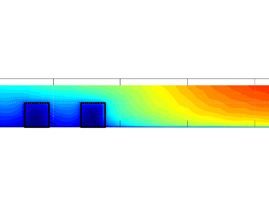
Figure 3 shows the cross-sectional distribution of the double-averaged longitudinal velocity  $\langle \bar {u} \rangle _x$. For the three test cases, there is, as expected, a high velocity difference between the smooth and rough subsections.

Figure 3. Cross-sectional distribution of double-averaged longitudinal velocity  $\langle \bar {u} \rangle _x$ for test cases SUB2, SUB1 and EMG.
The discharge in the rough and smooth subsections,  $Q_r$ and
  $Q_s$, is calculated by integrating
  $\phi \langle \bar {u} \rangle _x$ over each cross-section (the velocity in the white zones without measurements in figure 3 was extrapolated). The discharge ratio
  $Q_r/Q_{tot}$ is reported in table 2. It is seen to decrease from 24 % for SUB2 to 13 % for EMG. Table 2 also gives the subsectional effective bulk velocities
  $U_{e,r}=Q_{r}/A_{e,r}$ and
  $U_{e,s}=Q_{s}/A_{e,s}$, where
  $A_{e,r}$ and
  $A_{e,s}$ are the effective cross-sectional areas of the subsections (integral of
  $\phi$), the subsectional Reynolds numbers
  $\operatorname {Re}_r=hU_{e,r}/\nu$ and
  $\operatorname {Re}_s=hU_{e,s}/\nu$, and the subsectional Froude numbers
  $\operatorname {Fr}_r=U_{e,r}/(gh)^{0.5}$ and
  $\operatorname {Fr}_s=U_{e,s}/(gh)^{0.5}$.
Table 2. Subsectional flow quantities and non-dimensional numbers (index r refers to the rough and index s to the smooth subsection): the discharge ratio  $Q_r/Q_{tot}$; the subsectional effective bulk velocities
  $U_{e,r}=Q_r/A_{e,r}$ and
  $U_{e,s}=Q_s/A_{e,s}$, where
  $Q_r=\int _{y=-B}^{0} \int _{z=0}^{h} \phi \langle \bar {u} \rangle _x \, {\rm d} A$,
  $Q_s=\int _{y=0}^{B} \int _{z=0}^{h} \phi \langle \bar {u} \rangle _x \, {\rm d} A$,
  $A_{e,r}=\int _{y=-B}^{0} \int _{z=0}^{h} \phi \, {\rm d} A$,
  $A_{e,s}=\int _{y=0}^{B} \int _{z=0}^{h} \phi \, {\rm d} A$; the subsectional Reynolds numbers
  $\operatorname {Re}_r=hU_{e,r}/\nu$ and
  $\operatorname {Re}_s=hU_{e,s}/\nu$; the subsectional Froude numbers
  $\operatorname {Fr}_r=U_{e,r}/(gh)^{0.5}$ and
  $\operatorname {Fr}_s=U_{e,s}/(gh)^{0.5}$; the shear parameter
  $\lambda =(U_{2}-U_{1})/(U_{2}+U_{1})$; the definitions of
  $U_2$ and
  $U_1$ are given in the text.

Figure 4(a–c) shows, for different relative elevations  $z/k$, the lateral profiles of the double-averaged longitudinal velocity
  $\langle \bar {u} \rangle _x(y)$ and the lateral profiles of the streamwise-averaged longitudinal turbulent normal stress
  $\langle \overline {u'^2} \rangle _x(y)$ are shown in figure 4(d–f). The blue profiles for SUB2 and SUB1 are taken at mid-height of the fluid layer above the canopy and the red profiles are taken at mid-height of the cubes (
 $z/k=0.5$). The black dotted profile is the velocity additionally spatial-averaged in the lateral direction over a pattern length,
  $\langle \bar {u} \rangle _{x,y}(y)$. At the interface (around
  $y=0$), SUB2 and SUB1 feature the typical characteristics of a shear layer: a velocity profile with an inflection point and a peak of turbulence intensity. Concerning test case EMG, the velocity profile departs from the typical shear layer profile, as the velocity in the low-speed part is decreasing towards the high-speed part, instead of increasing. This atypical behaviour will be discussed later in this section.

Figure 4. (a–c) Lateral profiles of time- and  $x$-averaged longitudinal velocity (blue and red lines) and time-,
  $x$- and
  $y$-averaged longitudinal velocity (dashed black line) for the three test cases. (d–f) Same as panels (a–c) but for the longitudinal turbulent normal stress.
The shear parameter  $\lambda =(U_2-U_1)/(U_2+U_1)$ was calculated from the lateral profiles of
  $\langle \bar {u} \rangle _{x,y}(y)$ respectively at
  $z/k=1.50$,
  $z/k=1.25$ and
  $z/k=0.50$ for SUB2, SUB1 and EMG, and reported in table 2 (note that for SUB2 and SUB1,
  $\langle \bar {u} \rangle _{x,y}$ nearly collapses with
  $\langle \bar {u} \rangle _{x}$ at those
  $z$-elevations). Here,
  $U_2$ was taken as the maximum of
  $\langle \bar {u} \rangle _{x,y}$ in the smooth subsection, and
  $U_1$ as the value of
  $\langle \bar {u} \rangle _{x,y}$ around the fourth cube for SUB2 and SUB1, i.e. in the plateau region of
  $\langle \bar {u} \rangle _{x,y}$, and as the local minimum of
  $\langle \bar {u} \rangle _{x,y}$ for EMG, between the first and second cube. For all flows,
  $\lambda$ is much higher than 0.3, i.e. higher than the critical value
  $\lambda _{crit}$ which prevails for such flows for the onset of Kelvin–Helmholtz structures (see § 1).
The cross-sectional distribution of different turbulent stresses in the interface region is plotted in figures 5 and 6: the longitudinal turbulent normal stress  $\langle \overline {u'^2} \rangle _x$ in figure 5(a–c), the lateral turbulent normal stress
  $\langle \overline {v'^2} \rangle _x$ in figure 5(d–f), the lateral turbulent shear stress
  $\langle \overline {u' v'} \rangle _x$ in figure 6(a–c) and the lateral dispersive shear stress
  $\langle \tilde {\bar {u}} \widetilde {\bar {v}} \rangle _x$ in figure 6(d–f). As for the velocities, the turbulence stresses are normalised by the effective bulk velocity
  $U_e$. Other turbulent stresses which are not directly analysed in the paper are given in the Appendix.

Figure 5. (a–c) Longitudinal and (d–f) lateral  $x$-averaged turbulent normal stress in the
  $yz$-plane around the interface for test cases SUB2, SUB1 and EMG.

Figure 6. (a–c)  $x$-Averaged lateral turbulence shear stress and (d–f) lateral dispersive shear stress in the
  $yz$-plane around the interface for test cases SUB2, SUB1 and EMG.
Above the cube (for SUB2 and SUB1), a typical shear layer behaviour is observed, characterised by peaks of the turbulent stresses. Yet, the positions of maxima are different for the longitudinal and the lateral turbulent normal stresses. The maximum of  $\langle \overline {v'^2} \rangle _x$ is located right above the outer cubes, whereas the maximum of
  $\langle \overline {u'^2} \rangle _x$ is closer to the interface. For plane shear layers, the position of the peaks for the different turbulent stresses usually coincide, or are very close, and also coincide with the inflection point in the velocity profile (Bell & Mehta Reference Bell and Mehta1990; Olsen & Dutton Reference Olsen and Dutton2002; Loucks & Wallace Reference Loucks and Wallace2012). For shallow shear layers, however, the position of the peak can vary significantly for the different turbulent stresses (Dupuis et al. Reference Dupuis, Schraen and Eiff2023), mainly because several turbulent sources are present. Here, the wakes of the outer cubes, in particular the boundary layers on the upper faces, produce additional turbulence, which probably shifts the peak of the lateral turbulent normal stress.
For test case EMG, and below the cubes’ top for SUB2 and SUB1, the influence of the outer cubes is even stronger. The high  $\langle \overline {u'^2} \rangle _x$ with a maximum against the lateral cube face is likely due to the flow impingement against this face, especially the impingement of strong sweeps (lateral flow towards the low-speed side), which accompany the Kelvin–Helmholtz structures. In the region below the cubes’ top, the shear layer turbulence is therefore hidden by the turbulence from the cubes’ wake.
The lateral turbulent shear stress  $-\langle \overline {u'v'} \rangle _x$, shown in figure 6(a–c), gives the intensity and the direction of the lateral momentum transfer due to turbulent motion. For the submerged cases (SUB2 and SUB1), it is the strongest in the free-flow region above the cubes and the momentum transfer is towards the rough bed, i.e. towards the low-speed region. Below the cubes’ top, there is also a momentum transfer from the smooth side towards the cubes, although much weaker than the one above the cubes. Moreover, on the left-hand side of the outer cubes, a momentum transfer exists in the opposite direction, from the alley towards the cavity of the outer cubes. This momentum transfer is driven by the velocity gradient between the alley and the cavity, which is of opposite sign to that of the large-scale shear layer.
The lateral dispersive shear stress  $-\langle \tilde {\bar {u}} \tilde {\bar {v}} \rangle _x$, shown in figure 6(d–f), is another contributor to the lateral transfer of longitudinal momentum. In comparison with the turbulent shear stress, the dispersive shear stress is negligible (consider the scale in the figure) and is concentrated within and close to the cavity. The dispersive shear stress tends to transfer longitudinal momentum towards the cavity from both sides. It is due to recirculations and vortices developing in the cavity, which will be presented and discussed in § 6.1.
The fact that, in the present case, the dispersive shear stress is negligible outside of the canopy should not lead to the conclusion that it is a general case. It is known from boundary layer research that the extension of the roughness sublayer above the roughness crest, i.e. the region above the roughness crest where the dispersive shear stress still plays a role, is dependant on the geometry of the roughness. Very regular and dense canopies, for which the flow cannot reattach to the bottom between two successive roughness elements, induce a very weak dispersive shear stress outside the canopy (Chagot, Moulin & Eiff Reference Chagot, Moulin and Eiff2020). In the case of irregular canopies (Mignot, Hurther & Barthélemy Reference Mignot, Hurther and Barthélemy2009) or regular canopies for which the distance between the elements enables a reattachment of the flow to the bottom (Pokrajac et al. Reference Pokrajac, Campbell, Nikora, Manes and McEwan2007), the dispersive shear stress can be significant also outside the canopy. Pokrajac et al. (Reference Pokrajac, Campbell, Nikora, Manes and McEwan2007) for example showed that the dispersive shear stress still contributes significantly to the total stress even 2 $k$ above the canopy height, where
  $k$ is the height of the roughness elements. The negligible dispersive shear stress outside of the canopy in the present case is therefore related to the specific geometry of the roughness used.
Figure 7 summarizes the directions of the lateral and vertical transfers of longitudinal momentum in the interface region. The vertical transfers were determined by examining the vertical turbulent shear stress  $- \langle \overline {u'w'} \rangle _x$, shown in the Appendix. For the submerged cases SUB2 and SUB1, most of the lateral transfer of momentum occurs above the top of the outer cubes, and is directed towards the rough bed. The first alley is fed in longitudinal momentum from above (high
  $-\langle \overline {u'w'} \rangle _x$ in this region). The cavities of the outer cubes are fed in longitudinal momentum from the smooth side as from the first alley, through turbulent motion (turbulent shear stress) as well as through recirculations (dispersive shear stress). For the emergent case EMG, no momentum transfer can occur directly from the smooth bed to the alley, as the alley is isolated from the smooth bed by the cavities and there is no passage above the cubes.

Figure 7. Sketch of the fluxes of longitudinal momentum in the cross-section near the interface. Simple arrows indicate momentum transfers due to turbulence (turbulent shear stress) and double arrows momentum transfers due to recirculations (dispersive shear stress). For the purpose of representation, in this sketch, the view is from upstream and the flow is laterally mirrored (the smooth bed is on the right-hand side of the sketch).
Instantaneously however, momentum transfers do occur directly between the smooth bed and the alley in both directions, notably in form of large sweeps or ejections, as will be shown in § 6. However, averaged in time, the alley does not gain momentum from the cavity.
The cavities are fed by momentum from both sides. However, as there is no bulk longitudinal flow in the cavity, this momentum input is necessarily dissipated. It is converted into pressure force on the front face of the downstream cube and, to a lesser extent, into bottom friction and possibly into a suction force on the lee face of the upstream cube. In other words, the longitudinal momentum that enters the cavity is mostly lost by flow impingement against the face of the downstream cube.
For test case EMG, a particular flow pattern appears which departs from the expected shear layer behaviour. In figure 4(c), as mentioned above, the double-averaged velocity  $\langle \bar {u} \rangle _{x,y}$ on the low-speed side (cube array) decreases when approaching the high-speed smooth bed. Similarly, the peaks of
  $\langle \bar {u} \rangle _{x}$ in the alleys decrease when approaching the interface. This seeming anomaly can be explained as follows. Away from the shear layer and the interface, the flow in the canopy is characterised by strong and straight flows in the alleys. Close to the interface instead, turbulent large-scale structures (which will be analysed and discussed in more detail in § 5) generate strong lateral instantaneous flows through the canopy, especially in the first alley behind the outer cubes. These quasi-periodic transverse flows generate enhanced drag forces on the cubes (momentum loss), compared with the situation away from the shear layer and the interface. In addition, these transverse flows associated with quasi-periodic large-scale structures lead to the advection into the alley of the low-momentum fluid from the cavities, preventing the development of a straight and strong flow in the alley, and leading to velocities weaker than in alleys further away from the interface. In test cases SUB2 and SUB1, however, where this particular flow pattern is not observed, longitudinal momentum is additionally provided from above the canopy through vertical turbulent shear stress
  $-\overline {u'w'}$, which can compensate the effect of the large-scale periodic motions. This reversed velocity gradient within the shear layer was not observed in sparser canopies (White & Nepf Reference White and Nepf2007; Dupuis et al. Reference Dupuis, Proust, Berni and Paquier2017), likely because the channelisation of the flow in preferential alleys is not so strong in such cases.
4. Momentum balance in the smooth subsection
To quantify the interaction between the smooth bed and the cube array, a momentum balance can be carried out on either of the two subsections. Here, the momentum balance is performed on the smooth part of the channel ( $0< y< B$), which is easier, and reads, under the assumption of uniform flow:
 \begin{align} S_0 &= \underbrace{
\frac{1}{\rho g h B} \int_{y=0}^{B} (\tau_{xz})_{z=0}
\,{{\rm d} y} + \frac{1}{\rho g h B} \int_{z=0}^{h}
(\tau_{xy})_{y=B} \, {\rm d} z }_{S_{F}: \text{ friction}}
\underbrace{ - \frac{1}{\rho g h B} \int_{z=0}^{h}
(\tau_{xy})_{y=0} \, {\rm d}z }_{S_{T}: \text{ exchange by
turbulence}} \nonumber\\ &\quad + \underbrace{
\frac{1}{\rho g h B} \int_{z=0}^{h} (\rho \langle \bar{u}
\rangle_x \langle \bar{v} \rangle_x)_{y=0} dz }_{S_{SC}:
\text{ exchange by secondary currents}},
\end{align}
\begin{align} S_0 &= \underbrace{
\frac{1}{\rho g h B} \int_{y=0}^{B} (\tau_{xz})_{z=0}
\,{{\rm d} y} + \frac{1}{\rho g h B} \int_{z=0}^{h}
(\tau_{xy})_{y=B} \, {\rm d} z }_{S_{F}: \text{ friction}}
\underbrace{ - \frac{1}{\rho g h B} \int_{z=0}^{h}
(\tau_{xy})_{y=0} \, {\rm d}z }_{S_{T}: \text{ exchange by
turbulence}} \nonumber\\ &\quad + \underbrace{
\frac{1}{\rho g h B} \int_{z=0}^{h} (\rho \langle \bar{u}
\rangle_x \langle \bar{v} \rangle_x)_{y=0} dz }_{S_{SC}:
\text{ exchange by secondary currents}},
\end{align}
where  $\tau _{ij}$ is the total stress tensor, which is the sum of turbulent stress tensor, dispersive stress tensor and viscous stress tensor (see for example Nikora et al. Reference Nikora, Ballio, Coleman and Pokrajac2013):
 \begin{equation} \tau_{ij} =\rho \left( - \langle \overline{u'_i u'_j} \rangle - \langle {\widetilde{\overline{u_i}}\,\widetilde{\overline{u_j}}} \rangle + \frac{\nu}{\phi} \frac{\partial \phi \langle \overline{u_i} \rangle }{\partial x_j} \right) .\end{equation}
 As was seen above in figure 6, the dispersive stress in (4.2) is negligible at  $y=0$. As the viscous stress is also negligible, the exchange term
  $S_T$ only accounts for turbulent momentum exchange, the total shear stress being reduced to the lateral turbulent shear stress,
  $\tau _{xy}=-\rho \langle \overline {u'v'} \rangle _x$.
The momentum balance of (4.1) therefore states that the driving force (gravity force) which, once normalised, reduces to the slope  $S_0$, balances three terms: the friction force on the bed and the side wall
  $S_F$, the momentum flux coming from the cube array due to turbulent motion
  $S_T$ (which is here a sink of momentum) and the momentum flux coming from the cube array due to secondary currents
  $S_{SC}$ (which appears also to be a sink of momentum here). Secondary currents refer to the components of the time- and eventually space-averaged velocity vector that are in the cross-section plane (Tominaga & Nezu Reference Tominaga and Nezu1991; Nikora et al. Reference Nikora, Stoesser, Cameron, Stewart, Papadopoulos, Ouro, McSherry, Zampiron, Marusic and Falconer2019), i.e.
  $\langle \bar {v} \rangle _x$ and
  $\langle \bar {w} \rangle _x$.
The lateral turbulent shear stress at  $y=0$ could be directly calculated from the measurements. The secondary currents term
  $S_{SC}$ could also be calculated directly from the measurements. As the flow is considered to be uniform, there should be no bulk lateral velocity. Therefore, the depth-averaged lateral velocity,
  $\int _{z=0}^{h}(\langle \bar {v} \rangle _x )_{z=0} \, {\rm d} z$, which was not completely zero due to measurement inaccuracy, was first subtracted from
  $\langle \bar {v} \rangle _x$ to compute
  $S_{SC}$. Concerning the stress on the walls,
  $(\tau _{xz})_{z=0}$ and
  $(\tau _{xy})_{y=B}$, an estimate based on a Manning relationship was used, assuming that the wall shear stress
  $\tau _w$ is the same on the bottom and the side walls (all made of glass) and given by
 \begin{equation} \tau_w=\frac{\rho g n^2 U_{e,s}^2}{h^{1/3}},\end{equation}
where  $n$ is the Manning coefficient of glass (
 $n=0.0096\ {\rm s}\ {\rm m}^{-1/3}$). The value obtained for
  $\tau _w$ was close to the measured values of
  $-\rho \langle \overline {u'w'} \rangle _x$ and
  $-\rho \langle \overline {u'v'} \rangle _x$ in the vicinity of the bottom and the side wall, respectively (these measured quantities are hard to use directly to estimate the wall shear stress, as it is difficult to interpolate the total shear stress at the wall).
Figure 8 shows the contribution of the different terms of the momentum balance (4.1) for the three test cases. The fact that the budget is well balanced (the sum of the terms on the right-hand side of (4.1) approximately equals the slope  $S_0$) supports the hypotheses and approximations done for the momentum balance. The weight of the momentum exchange with the cube array (
 $S_T+S_{SC}$) increases with water depth. The contribution of the secondary currents in the momentum exchange (
 $S_{SC}$) appears to be very small, even zero for the case EMG. The momentum exchange between the two subsections is therefore mainly driven by the turbulent shear stress.

Figure 8. Momentum balance in the smooth subsection of the channel for the three test cases. The bars represent the different terms of (4.1), all normalised by the slope  $S_0$ and multiplied by 100. The blue bar is the slope itself (left-hand side of (4.1)), the green bar is the friction on the bottom and side wall, the red bar is the lateral exchange at
  $y=0$ due to turbulence and the yellow bar the lateral exchange at
  $y=0$ due to secondary currents.
The momentum balance highlights that for such flows, the interaction between adjacent subsections of different roughness has to be taken into account for an accurate prediction of the flow quantities, at least for the submerged cases. For the emergent case EMG, the weight of the momentum exchange with the adjacent bed remains quite small, such that in this case, a simple model as the divided channel method (isolated subsections) could be sufficient. It was seen indeed in the previous section that for EMG, the first row of cubes has the effect of blocking the momentum transfer towards the cube array, as would do a wall. In this case, the momentum transfer cannot cross the cavity.
The momentum exchange due to turbulent shear stress, which appears to be the dominant contribution of the dynamical interaction between the two beds, is known to be largely driven by turbulent coherent structures. These will be analysed in the next section.
5. Turbulent coherent structures
In the two preceding sections, the flow was analysed within the framework of the double-average approach. This approach, however, hides the underlying spatio-temporal turbulent structures, which are the focus of this section. Spatio-temporal correlation as well as coherent structure eduction will be considered.
Large spatio-temporal organised motions, also referred to as coherent structures (Hussain Reference Hussain1986), are a ubiquitous feature of turbulent flows. In the present flows, several coherent structures are a priori expected in the different canonical subflows – the boundary layer on the bed, the cube wakes and the shear layer. These are likely to interact with each other. In this section, we will focus on the primary structures of the shear layer, namely the Kelvin–Helmholtz structures, as the expected main contributor to the lateral momentum transfer.
5.1. Vertical coherence
As discussed in § 1, the coherence in the out-of-plane direction (here the vertical direction) of the Kelvin–Helmholtz structures remains an open question at large Reynolds numbers. Figure 9(a) shows simultaneous time series of the longitudinal velocity  $u(t)$ at different
  $z$-elevations and at
  $y=-3$ mm, i.e. close to the interface, for test case SUB2 (the time-resolved 2-D PIV measurements in vertical planes are used for this purpose). Comparing the signals at different
  $z$-elevations reveals that the large-scale fluctuations of the velocity signals are coherent across the whole water column, but also that smaller structures are superimposed to these large-scale fluctuations, especially near the bottom. This vertical correlation is confirmed by figure 9(b), which shows the maximum of correlation between the
  $u'(t)$-signal at a reference location near the surface (
 $z/h=0.86$) and the
  $u'(t)$-signal at lower
  $z/h$-locations,
  $R^{(3)}_{11,{max}}=max_{\tau } R^{(3)}_{11}(\tau )$. The correlation decreases with increasing vertical separation, but remains higher than 0.4, i.e. significant, even close to the bed.

Figure 9. (a) Time series of longitudinal velocity at  $x=56$ mm,
  $y=-3$ mm and at different
  $z$-elevations (mentioned on the plot) for test case SUB2; note that the vertical axis origin is shifted for each
  $z$-elevation. (b) Maximum of correlation between the
  $u'(t)$-signal at the reference location
  $z/h=0.86$ (the position of the horizontal dashed line) and the
  $u'(t)$-signal at lower
  $z$-locations. (c) Time lag for which the maximum of correlation is reached (a negative time lag indicates that the
  $u'(t)$-signal has a retardation compared to the reference
  $u'(t)$-signal at
  $z/h=0.86$).
The time lags for which the correlation maxima are reached,  $\tau ^{(3)}_{11,{max}}$, are reported in figure 9(c). It shows that statistically, the
  $u$-signal at lower
  $z$-elevations is retarded as compared to higher
  $z$-locations. This shifted phase when going down in the water column can also be observed in figure 9(a) for the rising edge occurring at approximately
  $t=3.4$ s at
  $z/h=0.86$ and at
  $t=3.8$ s at
  $z/h=0.05$.
Considering a constant convection velocity of the structures, estimated by the effective bulk velocity  $U_e$, the inclination angle
  $\alpha$ of the coherent structure with the vertical can be inferred from the phase shift of figure 9(c): if
  $\Delta \tau$ is the time lag over a vertical separation of
  $\Delta z$, then
  $\alpha \approx \operatorname {atan}(U_e \Delta \tau / \Delta z)$. Interpolating linearly
  $\tau ^{(3)}_{11,{max}}(z)$, the value obtained for this angle is 81
 $^\circ$, implying that the structures are very much inclined, their axis being almost horizontal. Similarly strong inclinations are also observed for the two other test cases, with very similar inclination angles (76
 $^\circ$ for SUB1 and 79
 $^\circ$ for EMG). A phase shift of the same sign and of very similar value (81
 $^\circ$) was also observed by Dupuis (Reference Dupuis2016) (p. 74) for Kelvin–Helmholtz structures in a compound channel shear layer. It should be noted though that the inclination of the structures, i.e. the inclination of their axes, does not imply that their vorticity vector is oriented along this axis. On the contrary, the velocity fluctuations are still maximum in the horizontal plane and the vorticity is mainly vertical.
It can be noticed that the inferred inclination angle of the Kelvin–Helmholtz structures with respect to the bottom (around 20 $^\circ$–25
 $^\circ$) is relatively close to the inclination angle of hairpin packets in turbulent boundary layers, which lies in the range 10
 $^\circ$–20
 $^\circ$ (Christensen & Adrian Reference Christensen and Adrian2001; Deng et al. Reference Deng, Pan, Wang and He2018). However, as the generation mechanisms of hairpin packets and of Kelvin–Helmholtz vortices are assumed to be quite different, it seems unlikely that there is a common explanation for these two inclination angles. Further investigations on the generation of Kelvin–Helmholtz vortices in shallow flows are necessary to shed light on the origin of their inclination.
The fact that the coherent structures are coherent across the water column would suggest at first sight that the convection velocity of the large-scale structure is also constant across the water column. However, there is an important vertical gradient of velocity. In figure 9(a), the mean velocity  $\langle \bar {u} \rangle _x$ is nearly multiplied by two between
  $z/h=0.05$ and
  $z/h=0.86$. In such conditions, how do the large-scale structures remain coherent in
  $z$ and are not torn apart by the strong shearing? Different explanations, listed below, can be given. They are not mutually exclusive.
• In the same way as the lateral gradient of velocity is due to the large-scale structure itself, as will be shown in figure 13, the vertical gradient of velocity could be explained by a 3-D configuration of the large-scale structure, for example a vortex of
 $y$-axis superposed to the main structure of Kelvin–Helmholtz type, constituting a complex 3-D topology.
• Another possibility would be that the large-scale structures, which are located in the interface region, are skewed laterally to follow iso-velocity lines. From figure 3, it can be seen that the iso-velocity lines in the interface region are laterally inclined with an angle of approximately 45
$^\circ$ (except very close to the bottom). It is possible that the coherent structures are also inclined with the same angle. In this case, the structures would not be sheared.• A third possible explanation is that the coherent structures are in fact longitudinally sheared due to the vertical velocity gradient, but they return to a more vertical position by branching and merging. In this view, a branched vortex line could merge with the vortex lines of the neighbouring vortices and, in this way, redress. Branched vortex lines were indeed observed by Browand & Troutt (Reference Browand and Troutt1985) in plane shear layers.


Further measurements and investigations would be necessary to validate or invalidate these hypotheses.
5.2. Pattern recognition technique
To obtain a visual representation of the typical Kelvin–Helmholtz structures that develop in the shear layers of the present flows, a PRT is used. This technique, developed by Ferre & Giralt (Reference Ferre and Giralt1989), consists in defining an initial pattern (called the template), for example a vortex of given size, and to detect all regions in the flow field that are sufficiently correlated with this pattern. The detected regions are then ensemble-averaged and this average is in turn used as new pattern. This procedure is repeated iteratively until it converges into a final pattern, which yields the dominant coherent structure of the flow (Ferre & Giralt Reference Ferre and Giralt1989).
The PRT was applied to the 2-D PIV measurements in the horizontal fixed planes. The turbulent structures to be educed are approximately 1.6 m in length, as was seen in figure 2, which is much longer than the field of view of the PIV (20 cm). Therefore, the PRT could not be applied to the PIV fields directly, and a preliminary step was to build a large-scale spatial flow field from the temporal field. To this end, Taylor's hypothesis was used. Starting with a spatio-temporal field along a single lateral line  $u(t,y)$ at a fixed
  $x$-position of the velocity field, a spatial field
  $u_T(x',y)$ was built (the index
  $T$ refers to Taylor's hypothesis), using a constant convection velocity
  $U_c$, taken as the double-averaged velocity at
  $y=0$ at that
  $z$-elevation:
  $x'=U_c t$, with
  $U_c= \langle \bar {u} \rangle (y=0,z)$.
In the PRT, the ensemble-averaging of all detected events is realised on a wider area than the pattern size. The final velocity field obtained is hereafter referred to as the ensemble-averaged field  $u_{EA}(x'',y'')$, where the coordinates
  $x''$ and
  $y''$ have their origin defined at the centre of the pattern. The number of detected events, and hence the number of samples to build the ensemble-average, varied between 154 and 232 for the different flows. Figure 10 summarises the different steps of the eduction method by the PRT.

Figure 10. Process to obtain the educed structure. The temporal velocity field along a lateral line  $u(t,y)$ is first transformed into a spatial field
  $u_T(x',y)$ using Taylor's hypothesis with a constant convection velocity
  $U_c$ taken as the double-averaged velocity at the interface at the given
  $z$-elevation. The PRT is then applied to this spatial velocity field, resulting in the ensemble-averaged field
  $u_{EA}(x'',y'')$, where the educed coherent structure appears. The coordinates
  $x''$ and
  $y''$ have their origin defined at the centre of the pattern.
It was verified that the results presented below are qualitatively not dependent on the choice of the convection velocity used in Taylor's hypothesis, nor on the correlation threshold used for the PRT (the correlation threshold for the detection was set at 60 %). Eiff & Keffer (Reference Eiff and Keffer1997) showed that, due to the iterative process, the result of the PRT does not depend on the details of the initial pattern (template), but instead depends on the size of this template. If the template is set too large, subharmonic scale structures, if present, can be filtered out. In the present case, the longitudinal size of the template was set to 0.5 m, i.e. approximately one third of the expected size of the structures. The lateral size of the template was set to 80 mm. Small variations around these sizes did not affect the results. The search for the structures was performed in the  $x'$-direction, but also in the lateral
  $y$-direction to allow for meandering positions.
It should be noted that the educed structures are not to be viewed as an exact representation of the instantaneous large-scale structures, since the conditions of validity of Taylor's hypothesis (see e.g. Zaman & Hussain Reference Zaman and Hussain1981), wherein the velocity fluctuations are assumed to be much smaller than the convection velocity and the term  $v \partial u / \partial y$ negligible compared to
  $\partial u / \partial t$, are not well fulfilled in the present case. In particular, the velocity fluctuations in the longitudinal and in the lateral direction are of the order of 50 % of the mean velocity. The large-scale lateral fluctuations are especially problematic because Taylor's hypothesis does not take into account lateral convection. In the present case, the term
  $v \partial u / \partial y$ (lateral convection) is of the same order of magnitude as
  $\partial u / \partial t$. Nevertheless, the results are expected to reveal the main features of these structures.
5.3. Educed coherent structures
Figure 11 shows the ensemble-averaged fields obtained for SUB2, SUB1 and EMG at  $z/h=0.81$, 0.75 and 0.63, respectively. In this figure, the convection velocity
  $U_c \boldsymbol {e}_x$ is subtracted from the velocity field. In these plots, a coherent structure appears in the ensemble-averaged flow field, having the topology of the Kelvin–Helmholtz structure, i.e. a succession of vortices and saddle points. The structure is also observed at the other
  $z$-elevations measured across the water depth, which are as close as 1 cm from the bed (not shown). However, for the
  $z$-elevations below the cube top (as in figure 11c), the structure is less perceptible. This is due to the fact that the structure penetrates and interacts with the cube array (see § 6), while the PRT could not be carried out in the cube array. Indeed, a velocity field reconstruction based on Talyor's hypothesis is not possible there, due to the presence of the cubes.

Figure 11. Velocity field ( $u_{EA}-U_{c},v_{EA}$) of the ensemble-averaged field obtained by PRT in the horizontal plane for test case (a) SUB2 at
  $z/h=0.81$, (b) SUB1 at
  $z/h=0.75$ and (c) EMG at
  $z/h=0.63$. The dashed rectangle indicates the size of the template.
The PRT detection does not necessitate the large-scale structures to be quasi-periodic. Nevertheless, a quasi-periodicity is observed in the ensemble-averaged fields of figure 11. In particular, the saddle point, which in all cases is close to the middle of the field, is flanked by two vortices – exceeding the size of the template. The periodicity is not very strong, as exemplified by the difference between these two vortices right and left from the saddle point (having different shapes and lateral positions). The relative lack of periodicity can be explained by the variability in the individual structures’ size (in the ensemble-averaging, the small and big structures are averaged together, such that the correlation between the detected structures becomes weak when going away from the middle of the pattern).
To illustrate this variability in structures’ size, figure 12 shows, for test case SUB2 at  $z/h=0.81$, the distribution of the separation distance between two detected events,
  $\Delta x_{detection}$, which gives an estimate of the distribution of the length of the structures. Equating separation distance with size assumes that there is no structural intermittency in the interface region, i.e. that the velocity signal is always coherent and not a succession of coherent sequences followed by chaotic fluctuations (Fiedler Reference Fiedler1988). This assumption was fulfilled here. As can be seen in figure 12, most structures have a length of approximately 1.5 m, as expected from figure 2, but the range of variations lies between 1 and 3 m. The distribution of
  $\Delta x_{detection}$ was qualitatively similar for the other
  $z$-elevations and the other test cases, with typically a factor 3 to 4 between the largest and the smallest structures.

Figure 12. Distribution of the longitudinal separation distance between two detected events for test case SUB2 at  $z/h=0.81$.
5.4. Contribution of the educed coherent structure to mean flow and turbulence
To estimate the contribution of the educed coherent structure to the overall flow, the ensemble-averaged flow field  $u_{EA}$ of test case SUB2 was
  $x$-averaged in space between
  $x''=-750$ and 750 mm, i.e. approximately the length of the periodic pattern. The obtained velocity
  $\langle u_{EA} \rangle _{x''}$ is plotted in figure 13(a) at
  $z/h=0.81$ and compared with the double-averaged velocity of the original flow field
  $\langle \bar {u} \rangle _x$. Similarly, the same was done for the turbulent stresses
  $\rho \langle \tilde {u}_{EA}^2 \rangle _{x''}$,
  $\rho \langle \tilde {v}_{EA}^2 \rangle _{x''}$ and
  $\rho \langle \tilde {u}_{EA} \tilde {v}_{EA} \rangle _{x''}$, which were compared with
  $\rho \langle \overline {u'^2} \rangle _x$,
  $\rho \langle \overline {v'^2} \rangle _x$ and
  $\rho \langle \overline {u'v'} \rangle _x$. For the quantities derived from the spatial averaging of the ensemble-averaged field, the lateral coordinate
  $y''$ was shifted by a value
  $y_{shift}$, chosen such that the maximum of turbulence is at the same
  $y$-position as for the original flow.

Figure 13. Lateral profiles of mean velocity and turbulent stresses for test case SUB2 at elevation  $z/h=0.81$, obtained either by averaging in
  $x$ the ensemble-averaged field delivered by the PRT (red curves) or by double-averaging the original measured flow field (blue curves).
As shown in figure 13(a), the component  $\langle u_{EA} \rangle _{x''}(y''+y_{shift})$ of the educed coherent structure yields the shape and almost the same magnitude as
  $\langle \bar {u} \rangle _x(y)$. The Kelvin–Helmholtz structure educed with a constant convection velocity therefore accounts by itself for the lateral gradient of velocity at the interface.
Concerning the turbulent stresses shown in figures 13(b–d), it can be seen that the velocity fluctuations associated with the educed coherent structure,  $\rho \langle \tilde {u}^2_{EA} \rangle _{x''}$,
  $\rho \langle \tilde {v}^2_{EA} \rangle _{x''}$ and
  $\rho \langle \tilde {u}_{EA} \tilde {v}_{EA} \rangle _{x''}$, are responsible for approximately
  $35\,\%$ of
  $\rho \overline {u'^2}$ and
  $60\,\%$ of
  $\rho \overline {v'^2}$ and
  $\rho \overline {u'v'}$, respectively.
While the fluctuations associated with the educed structure reproduce, to a large extent, the shape of the turbulent stresses, in particular for  $\rho \langle \overline {u'^2} \rangle _x$ and
  $\rho \langle \overline {u'v'} \rangle _x$ (figures 13b and 13d), the peak in
  $\rho \langle \overline {v'^2} \rangle _x$ appears more pronounced and shifted to the left compared with
  $\rho \langle \tilde {v}^2_{EA} \rangle _{x''}$ (figure 13c). In other words, there is an additional peak in
  $\rho \langle \overline {v'^2} \rangle _x$ at
  $y/B \approx -0.08$ above the cubes that is not due to the coherent structure (the peak in
  $\rho \langle \overline {v'^2} \rangle _x$ can also be observed in figure 5d). It is therefore surmised that this excess energy in
  $\rho \langle \overline {v'^2} \rangle _x$ is due to another source of turbulence, namely the cube wakes. The difference in peak position of the turbulence intensities, which was observed in § 3, can then be attributed to the fact that two sources of turbulence interact here and determine together the overall turbulence intensity.
Finally, it should be noted that the contribution to mean flow and turbulence of the educed coherent structure presented in figure 13 does not take into account the variation of size of the individual structures. This dispersive effect would enhance the contribution of the coherent structure to the overall turbulence.
Figure 14 gives the power spectral density (PSD) of the time series of the longitudinal and lateral velocity fluctuations  $u'(t)$ and
  $v'(t)$ for test case SUB2 at
  $z/h=0.81$ in the interface region (
 $y/B=0.035$). The frequencies corresponding to the length scale of the smallest and largest detected structures (1 and 3 m), identified in figure 12, are also reported (the conversion into frequency is made by means of Taylor's hypothesis with convection velocity
  $U_{c}$), as well as the integral time scale
  $\tau _u$ derived from the autocorrelation (plotted in figure 2). It can be observed that the spectral region corresponding to the variation range of the length of the coherent structures is characterised by a departure from the
  $-5/3$ slope (the inertial region), with an increase of the slope. For comparison, the
  $-3$ slope, which Uijttewaal & Jirka (Reference Uijttewaal and Jirka2003) identified to characterise quasi-2-D structures in shallow flows, is depicted in the figure. The peak frequency of the spectra is the same as that given by the integral time scale
  $\tau _u$. The broadness of the peak region is a characterising feature of quasi-periodicity and can be explained by the scatter in the size of the individual structures.

Figure 14. Power spectral density (PSD) of the fluctuations of the longitudinal (blue line) and lateral (red line) velocity for test case SUB2 at  $z/h=0.81$,
  $y/B=0.035$ and
  $x/B=0.11$. The vertical dotted lines depict the size range of the coherent structures between 1 and 3 m (converted to frequency using
  $U_{c}$ as convection velocity), and the integral time scale
  $\tau _u$ inferred from the auto-correlation of
  $u(t)$ (figure 2).
6. Coupling between coherent structures and obstacle wake
This section aims at providing evidence that there exists a dynamic coupling between the passage of the Kelvin–Helmholtz structures and the wakes of the outer cubes. To this end, the time-average flow around the outer cube is analysed first. All of § 6 will be restricted to test case SUB2. The results are very similar for test case SUB1. For test case EMG, the time-averaged flow pattern around the cube is different from the submerged cases, but the coupling between Kelvin–Helmholtz structure and wake is similar. The interaction with the other cubes (farther from the interface) is not investigated, but is expected to be much weaker.
6.1. Time-averaged flow pattern around the outer cube
The time-averaged flow pattern around an isolated, surface-mounted cube is characterised by the following main features (Larousse, Martinuzzi & Tropea Reference Larousse, Martinuzzi and Tropea1991): (i) a separation of the boundary layer upstream of the cube, with generation of a horseshoe vortex in the recirculation region, whose legs extend far downstream on each side of the cube; (ii) an arch vortex on the downstream side of the cube; (iii) local separation and reattachment on the top and side faces of the cube, giving rise to small recirculation bubbles. Concerning the arch vortex at the rear face of the cube (point ii), it remains an open question if it is really a closed vortex forming an arch, or if it is formed by two disconnected counter-rotating vortices with one end at the channel floor and the other end being diffused in the shear flow above the cube (Meinders & Hanjalić Reference Meinders and Hanjalić1999).
In the case of an array of cubes in a square configuration, Meinders & Hanjalić (Reference Meinders and Hanjalić1999) showed that if the longitudinal distance between two cubes is sufficient for the flow to reattach between the cubes, then the flow pattern is essentially the same as for the isolated cube, except that the vortices, especially the horseshoe vortex, can interact with those of the neighbouring cubes. When the longitudinal gap between the cubes becomes of the order of the cube size (as is the case in the present study), the flow cannot reattach on the floor between two cubes and the time-averaged flow in the inter-cube space (the cavity) is characterised by a recirculation cell of  $y$-axis, which occupies the whole cavity, and by two symmetric
  $z$-axis vortices (Coceal et al. Reference Coceal, Thomas, Castro and Belcher2006). In this case, there is no horseshoe vortex and the time-averaged velocities in the cavity are very small (dead-water region).
Figure 15 shows the velocity field in the vertical  $xz$-plane at a lateral position corresponding to the middle of the cube, for test case SUB2. As in the case of the laterally invariant cube array (Coceal et al. Reference Coceal, Thomas, Castro and Belcher2006, their figure 12), there is a recirculation cell of
  $y$-axis that spans the whole cavity.

Figure 15. Time-averaged velocity field ( $\bar {u},\bar {w}$) in the
  $xz$-plane at the position
  $y/B=-0.0818$ (middle of the cube) for test case SUB2.
The velocity field in horizontal  $xy$-planes is shown in figure 16 at three
  $z$-elevations. Consider first the elevation at mid-height of the cube (
 $z/k=0.5$), for which figure 16(g) shows the topology that was inferred from the velocity field and the streamlines (figures 16b and 16e). Here the topological rules (Hunt et al. Reference Hunt, Abell, Peterka and Woo1978; Foss Reference Foss2004; Foss et al. Reference Foss, Hedden, Barros and Christensen2016) were verified to be fulfilled: the domain sketched in figure 16(g) is a collapsed sphere (in the sense of Foss Reference Foss2004) with four holes and no handles (the lateral extension of the domain can be chosen such that it is laterally closed by streamlines), such that the Euler characteristic is
  $\chi =2-\sum \text {holes}- 2 \sum \text {handles}=-2$; therefore, the following relation should hold:
  $2\sum N + \sum N' - 2\sum S - \sum S'=\chi =-2$, where
  $N$ are nodes,
  $N'$ half-nodes,
  $S$ saddle points and
  $S'$ half-saddle points (there is no obtuse angle in this case, see Foss et al. Reference Foss, Hedden, Barros and Christensen2016). The flow field at
  $z/k=0.5$ (figures 16b, 16e and 16g) differs significantly from the laterally invariant cube array case (Coceal et al. Reference Coceal, Thomas, Castro and Belcher2006, their figure 14): the two counter-rotating
  $z$-axis vortices N1 and N2 are still present but are not symmetric, and a third vortex N3 appears upstream of the cube on the high-speed side. Additionally, two saddle points, S1 and S2, are present.

Figure 16. (a–c) Time-averaged velocity field ( $\bar {u},\bar {v}$) and (d–f) corresponding streamlines in the
  $xy$-plane at vertical positions (a,d)
  $z/k=0.87$, (b,e)
  $z/k=0.50$ and (c, f)
  $z/k=0.12$ for test case SUB2. Panel (g) is the interpreted flow topology of panel (e).
The flow is similar closer to the bottom, at  $z/k=0.12$ (figures 16c and 16f). The three vortices can still be identified (which are now repelling or attracting focuses) as well as the two saddle points. Close to the cube top, at
  $z/k=0.87$ (figures 16a and 16d), the vortices and saddle points have disappeared and solely the top of the recirculating cell of
  $y$-axis can be seen (that which was observed in figure 15). Observations at intermediate planes showed that, as claimed by Meinders & Hanjalić (Reference Meinders and Hanjalić1999), it does not seem that the two counter-rotating vortices at the rear face of the cube connect to form an arch.
For test case SUB1, the time-average flow pattern around the outer cube is exactly the same as for SUB2. For test case EMG however, there is neither a  $y$-axis recirculation in the cavity, nor vertical columnar vortices.
6.2. Phase-averaged flow pattern around the outer cube
To identify if there is a coupling between the passage of the Kelvin–Helmholtz structures and the flow around the outer cube, a phase-average is carried out in the horizontal  $xy$-plane
  $z/k=0.5$ around the outer cube for test case SUB2. In contrast to the preceding section dedicated to the eduction of the coherent structures, here it is not necessary to reconstruct the flow field using Taylor's hypothesis, since the PIV field of view is large enough to capture the outer cube's wake. The errors introduced by Taylor's hypothesis are thus avoided. For detecting the passage of the individual Kelvin–Helmholtz structures, a simpler method than in the preceding section was implemented, namely a detection based on a trigger, as described for example by Wallace, Brodkey & Eckelmann (Reference Wallace, Brodkey and Eckelmann1977). Figure 17 shows the time series of the lateral velocity
  $v(t)$ at
  $z/k=0.5$ at the interface
  $y=0$. At this location, the periodicity of the lateral velocity fluctuation due to the passage of the Kelvin–Helmholtz structures is quite marked and can therefore be used as a trigger for the phase-average. To this end, the signal was first smoothed with a moving average of time span 1.5 s (black line in figure 17) to define the maxima (circles) which are used to indicate a given phase of the passage. The time between two of these
  $v$-maxima is considered as a period. As there is no structural intermittency, the end of a given period is also the beginning of the next one. Each period is then divided into 20 phases. The flow is averaged within each phase and over all detected periods, resulting in the field
  $(u_{PA,i},v_{PA,i})$ (
 $PA$ stands for phase-average and
  $i$ is the number of the phase).

Figure 17. Time series of the lateral velocity  $v$ (grey line) for test case SUB2 at
  $z/k=0.5$ and
  $y=0$, and its smoothed signal (black line) used for detecting a constant phase in the phase-averaging process. The circles indicate the detections (local maximum).
Figure 18(a) shows the resulting phase-averaged value of lateral velocity  $v_{PA,i}$ at
  $y=0$,
  $x/B=0.1$ and
  $z/k=0.5$ as a function of phase
  $i$: phases 1 and 20 correspond to the maximum of
  $v_{PA,i}$, phase 10 to the minimum of
  $v_{PA,i}$. The passage of the vortex centre of the coherent structure corresponds approximately to phase 3 (at the centre of the vortex,
  $v$ is zero and goes from negative to positive values) and the passage of the saddle point approximately to phase 18 (
 $v$ is zero and goes from positive to negative).

Figure 18. (a) Phase-averaged lateral velocity  $v_{PA,i}$ at
  $y=0$,
  $x/B=0.1$ and
  $z/k=0.5$ as a function of phase
  $i$. (b) Lateral velocity averaged over the cavity length,
  $v_{cavity}$, as a function of the phase at
  $z/k=0.5$. The letters A, B and C refer to the three different topologies that succeed during the passage of the structure.
Observation of the 20 phase-averaged flow fields at  $z/k=0.5$ reveals that three different flow topologies succeed during the passage of the structure, denoted A, B, and C. Topology A lasts from phase 1 to 3, B from 4 to 16, C from 17 to 20, as reported in figure 18(a) by vertical lines. To visualise this, the phase-averaged flow fields obtained for the phases 1, 4, 14 and 18 are shown in figure 19. The corresponding streamlines and the inferred topology are also shown (as in figure 16g, the topological rules were verified to be fulfilled, i.e. here
  $\chi =-2$). Phase 1, for which
  $v$ is maximum and topology A holds, is characterised by two vortices (N1 and N2) and one saddle point (S1) in the cavity. Fluid is able to flow through the cavity towards the high-speed side. Around phase 3, a bifurcation between the topologies A and B takes place: a reversal of the flow occurs along the cube wall on the downstream side of the cavity. This causes the saddle point S1 to disappear and the saddle point S2 to appear (it is not S1 which moves towards the low-speed side; S1 and S2 are fundamentally different as one of the divergent separatrices is going in one case left of the downstream cube and in the other case right of it). Topology B (phase 4 in figure 19) allows fluid to flow through the cavity in both the positive and the negative
  $y$-directions, but mainly towards the low-speed side (negative
  $y$). This topology remains unchanged until phase 16 (the changes concerning the half-saddle points S’1 and S’2 between phases 4 and 14 in figure 19 are not significant). However, the vortex N1 progressively moves downstream (figures 19b and 19c). Around phase 16, a new bifurcation occurs, wherein the saddle point S2 and the vortex N1 disappear such that a strong cross flow towards the high-speed side can develop (topology C, shown in phase 18 in figure 19). At phase 20, a third bifurcation occurs, where the vortex N1 and the saddle point S1 are rebuilt (leading back to topology A).

Figure 19. Phase-averaged flow field in the  $xy$-plane obtained for the phase
  $i=1$, 4, 14 and 18 for test case SUB2 at
  $z/k=0.5$: (a–d)
  $(u_{PA,i},v_{PA,i})$-field, (e–h) streamlines, (i–l) flow topology.
The time-averaged flow field of the outer cube's wake, as depicted in figure 16(b,e,g), never occurs in the phase-averaged flows of figure 19, which are closer to the instantaneous flow. While there are three vortices and two saddle points in the time-averaged flow field, there are at most two vortices and one saddle point in the phase-averaged flow field. In the time-averaged flow field, no flow crosses the cavity, because of the separatrice between the two half-saddle points S’1 and S’4, which closes the cavity. Yet, in the phase-averaged flow, the cavity is always open, and for some phases, strong cross-flows are present (e.g. phase 18 with topology C).
To estimate the intensity of the cross-flow across the cavity, the net lateral velocity in the same plane  $z/k=0.5$, averaged in the streamwise direction over the cavity length at
  $y/B=-0.08$,
  $v_{cavity}$, is shown in figure 18(b) as a function of the phase
  $i$. Important cross-flow variations dominate the cavity dynamics, with velocity fluctuations of
  ${\pm }5\ {\rm cm}\ {\rm s}^{-1}$, i.e. even higher than the
  $v$-fluctuations at
  $y=0$ (figure 18a). An asymmetry can also be observed between the positive and negative phase of
  $v_{cavity}$: the negative phase (corresponding to sweeps, flow towards the canopy) is longer and associated with lower velocities, whereas the positive phase (corresponding to ejections, flow towards the smooth region) is shorter and associated with much higher velocities.
Finally, it can be noted that the bifurcation between topology A and B corresponds to the passage of the vortex core of the Kelvin–Helmholtz structure (phase 3), whereas the bifurcation between topology B and C corresponds approximately to the passage of the saddle point (phase 16).
7. Conclusion
Open-channel flows with a lateral variation of bed roughness were investigated experimentally using a newly developed telecentric scanning 3-D-2-C PIV technique. The roughness elements consisted in an array of cubes placed on a smooth bottom and the water levels were set to two lowly submerged conditions and one emergent condition. With this particular roughness geometry, the measurement technique used was able to measure and resolve nearly the full width of the flow, including the flow in the interstices between the roughness elements. The mean flow and turbulence could be characterised in terms of double-averaged quantities, and coherent structure eduction could be carried out by means of a pattern recognition technique. In addition, a phase-average between the large-scale structures and the interstitial flow around the cubes was implemented. The flow pattern is quite complex because several flow phenomena are present and interact with each other: shear layers, boundary layers, wakes.
The interaction between the rough and the smooth subsections contributes strongly to the momentum balance of the smooth subsection, except for the case with emergent cubes. For the investigated flows, this momentum exchange is nearly exclusively due to turbulent motion, whereas secondary currents play a minor role, and the contribution of dispersive stress at the interface is completely negligible.
The analysis of the direction of the momentum flux across the cross-section shows that the cube canopy itself is not fed by momentum directly from the smooth bed, as it is isolated from it by the first row of cubes (see sketch of figure 7), through which the momentum cannot pass. For the submerged cases, the canopy is only supplied by momentum from the flow above it. For the emergent case, the canopy is completely isolated from the smooth part (except the first cavity).
Special attention was paid on the large-scale structures that are present in the shear layer at the interface between the two subsections. These large-scale structures were educed using a pattern recognition technique (PRT) in horizontal planes. The Kelvin–Helmholtz topology (succession of vortices and saddle points) was observed from the water surface to very close to the bottom (1 cm above the bed). It was established that the structures are coherent over the whole water column. However, they travel with a strong vertical inclination, such that the higher part has a phase advance compared with the lower part.
The coherent structures are quasi-periodic, with a broad range in the size of the individual structures (typically a factor 3 to 4 between the largest and the smallest). This is reflected by a broad peak in the power spectra. The scatter in the length of the structures is likely due to dynamical mechanisms such as merging and splitting of the individual structures (Winant & Browand Reference Winant and Browand1974), as well as entrainment effects and nibbling (da Silva et al. Reference da Silva, Hunt, Eames and Westerweel2014). These dynamical mechanisms are also usually put forward to explain the overall growth of the large-scale structures, which was observed in the present case all along the channel (figure 2).
The coherent structure pattern that was educed using the pattern recognition technique accounts by itself for the lateral profile of the time-averaged velocity  $\langle \bar {u} \rangle _x(y)$ in the interface region. From this point of view, the large-scale structures (educed with a constant convection velocity) are not sheared by the lateral gradient of velocity, since this velocity gradient is due to the large-scale structures themselves. The educed coherent structure is also responsible for a large part of the turbulent stresses. In particular, it contributes to approximately 60 % to the turbulent shear stress.
A coupling was identified between the passage of the coherent structures and the flow around the cubes at the interface with the smooth bed (outer cubes). The coherent structures induce a quasi-periodic cross-flow in the cavity, characterised by strong lateral movements in both directions, repeatedly washing out the cavity. The phase-averaged flow is therefore very different from the time-averaged flow, for which the cavity appears as a dead-water zone.
This interaction between the large-scale structures and the cubes’ wake leads to an unexpected phenomenon, which was observed in the double-averaged streamwise velocity for the test case with emergent cubes (figure 4): in the cube array, the velocity decreases when approaching the high-speed smooth bed. The given explanation is that the large-scale structures are perturbing the flow within the free alley between the first two rows of cubes. In this alley, no straight fast flow can develop, unlike what occurs away from the interface.
In these complex flows, three sources of turbulence production can be identified: the boundary layer on the walls, the wake of the cubes and the shear layer. However, it would be impossible and have little sense to determine the contribution of each of them to the overall turbulence. First because even if these turbulence sources are associated with different length scales, the spectral ranges of these turbulent length scales overlap largely, such that they cannot be separated by signal analysis. Second, these turbulent sources interact with each other, as illustrated by the coupling between shear layer and wake flow (the Kelvin–Helmholtz structures generating an extra cross-flow around the cube, which therefore enhances the wake turbulence), such that they are not independent sources. The contribution that could be separated was that due to the large-scale Kelvin–Helmholtz structures. This separation was facilitated by the spectral separation with the other turbulence sources. Yet, the shear layer, and the Kelvin–Helmholtz structures themselves, are also inducing smaller-scale turbulence, especially through secondary instabilities, which also contributes to the turbulent stresses.
A limitation of the eduction methods of coherent structures is that they deliver a static image of the coherent structure. In reality, these structures, as mentioned above, evolve with the flow by growing, decaying or interacting with neighbouring structures.
Acknowledgements
We are grateful to J.-D. Barron, S. Cazin and M. Marchal for their technical support and advice.
Funding
The work was funded by the European Union (Hydralab+ project) and by the French National Research Agency (Flowres project, grant no. ANR-14-CE03-0010). The PIV data were processed at the academic supercomputing centre CALMIP in Toulouse.
Declaration of interests
The authors report no conflict of interest.
Appendix. Additional fields of turbulent quantities
In this appendix, some plots of turbulent quantities, which were not directly analysed in the article, but could be of interest for the reader, are presented.
Figures 20 and 21 show respectively the cross-sectional distribution of the  $x$-averaged vertical turbulent normal stress
  $\langle \overline {w'^2} \rangle _x$ and of the vertical turbulent shear stress
  $\langle \overline {u' w'} \rangle _x$.

Figure 20.  $x$-Averaged vertical turbulent normal stress in the
  $yz$-plane for test cases SUB2, SUB1 and EMG.

Figure 21.  $x$-Averaged vertical turbulent shear stress in the
  $yz$-plane for test cases SUB2, SUB1 and EMG.
Figures 22 and 23 show different turbulent stresses in the horizontal  $xy$-plane at mid-height of the cube
  $z/k=0.5$. Figure 22 comes from the lateral scanning and spans therefore a broader flow region than figure 23, which comes from the vertical scanning. It can be observed in particular that the effect of the flow impingement against the upstream face of the cube is to create high lateral and vertical turbulence intensity (while the longitudinal turbulence intensity is very low). This effect of flow impingement on the turbulence was already observed by Meinders & Hanjalić (Reference Meinders and Hanjalić1999) and in the DNS of a single cube of Yakhot, Liu & Nikitin (Reference Yakhot, Liu and Nikitin2006).

Figure 22. (a,b) Longitudinal turbulent normal stress, (c,d) vertical turbulent normal stress and (e, f) vertical turbulent shear stress at  $z/k=0.5$ for (a–c) test case SUB2 and (d–f) test case EMG.

Figure 23. (a) Longitudinal turbulent normal stress, (b) lateral turbulent normal stress and (c) lateral turbulent shear stress at  $z/k=0.5$ for test case SUB2.
Similarly, the high longitudinal and vertical turbulence intensity (and low lateral turbulence intensity) on the high-speed-side side-face of the outer cube can be explained by impingement of sweeps against this face (cross-flow towards the cube array) generated by the shear layer.


 Open access