


1. Introduction
Turbulent flows laden with particles are present in both environmental phenomena and industrial applications. For instance, water droplets, snowflakes and pollutants in atmospheric turbulence, sediments in rivers and industrial sprays all involve turbulent environments carrying inertial particles (Crowe, Troutt & Chung Reference Crowe, Troutt and Chung1996; Shaw Reference Shaw2003; Monchaux, Bourgoin & Cartellier Reference Monchaux, Bourgoin and Cartellier2012; Li et al. Reference Li, Lim, Berk, Abraham, Heisel, Guala, Coletti and Hong2021). Inertial particles do not follow the fluid velocity field as tracers, having their own dynamics that depend on both their finite size and their density ratio compared with that of the carrier phase.
Two phenomena resulting from the influence of turbulence on the motion of inertial particles have been widely studied: preferential concentration and modification of the settling velocity. Preferential concentration refers to the fact that an initially uniform or random distribution of particles will form areas of clusters and voids (Maxey Reference Maxey1987; Squires & Eaton Reference Squires and Eaton1991; Aliseda et al. Reference Aliseda, Cartellier, Hainaux and Lasheras2002; Obligado et al. Reference Obligado, Teitelbaum, Cartellier, Mininni and Bourgoin2014; Sumbekova et al. Reference Sumbekova, Cartellier, Aliseda and Bourgoin2017) due to the accumulation in certain regions of the turbulent flow where the hydrodynamic forces exerted by the flow tend to drive the particles. Furthermore, settling velocity modification occurs when particles immersed in a turbulent flow have their settling speed  $V_s$ altered compared with that in a stagnant fluid or laminar flow
  $V_T$ (Wang & Maxey Reference Wang and Maxey1993; Crowe et al. Reference Crowe, Troutt and Chung1996; Aliseda & Lasheras Reference Aliseda and Lasheras2011). These two features of turbulent-laden flow are known to be linked together as the settling velocity of a particle can be increased due to an increase of the particle local concentration (Aliseda et al. Reference Aliseda, Cartellier, Hainaux and Lasheras2002; Gustavsson, Vajedi & Mehlig Reference Gustavsson, Vajedi and Mehlig2014; Huck et al. Reference Huck, Bateson, Volk, Cartellier, Bourgoin and Aliseda2018).
Regarding the modification of the settling velocity, multiple experimental and numerical studies have shown that turbulence can both hinder  $(V_s < V_T)$ or enhance the particle settling velocity
  $(V_s > V_T)$. While several studies have reported enhancement of the settling velocity (Wang & Maxey Reference Wang and Maxey1993; Aliseda et al. Reference Aliseda, Cartellier, Hainaux and Lasheras2002; Bec, Homann & Ray Reference Bec, Homann and Ray2014; Rosa et al. Reference Rosa, Parishani, Ayala and Wang2016; Monchaux & Dejoan Reference Monchaux and Dejoan2017; Falkinhoff et al. Reference Falkinhoff, Obligado, Bourgoin and Mininni2020), others show evidence of hindering only (Akutina et al. Reference Akutina, Revil-Baudard, Chauchat and Eiff2020; Mora et al. Reference Mora, Obligado, Aliseda and Cartellier2021) or of both types of modification (Nielsen Reference Nielsen1993; Good, Gerashchenko & Warhaft Reference Good, Gerashchenko and Warhaft2012; Sumbekova et al. Reference Sumbekova, Aliseda, Cartellier and Bourgoin2016; Petersen, Baker & Coletti Reference Petersen, Baker and Coletti2019). While the nature and number of mechanisms controlling this phenomenon is still a matter of debate, several models have been proposed in the literature, sometimes even giving contradictory predictions.
Enhancement of the settling velocity can be explained by the preferential sweeping mechanism, also known as the fast-tracking effect, where inertial particles tend to spend more time in downwards moving regions of the flow than in upwards flow (Wang & Maxey Reference Wang and Maxey1993). Some mechanisms have been proposed as well to explain hindering. The vortex trapping effect describes how light particles can be trapped inside vortices (Nielsen Reference Nielsen1993; Aliseda & Lasheras Reference Aliseda and Lasheras2006). The loitering mechanism assumes that falling particles spend more time in upward regions of the flow than downward regions (Chen et al. Reference Chen, Liu, Chen and Wang2020), while a nonlinear drag can also explain that particles are slowed down in their fall by turbulence (Good et al. Reference Good, Ireland, Bewley, Bodenschatz, Collins and Warhaft2014). Models have been developed to estimate the influence of clustering and particle local concentration on the settling rate enhancement (Alipchenkov & Zaichik Reference Alipchenkov and Zaichik2009; Huck et al. Reference Huck, Bateson, Volk, Cartellier, Bourgoin and Aliseda2018).
However, even in the simplified case of small, heavy particles in homogeneous isotropic turbulence (HIT) no general consensus has been found on the influence of turbulence, through the Taylor-scale-based number  $Re_\lambda$, on the transition between hindering and enhancement. The Taylor–Reynolds number
  $Re_\lambda = u'\lambda /\nu$ is based on the Taylor microscale
  $\lambda$ where
  $u'$ and
  $\nu$ are the carrier phase root-mean-square (r.m.s.) of the fluctuating velocity and kinematic viscosity, respectively. The influence of
  $Re_\lambda$ on the maximum of enhancement, i.e. when
  $V_s - V_T$ reaches its maximum, is also still under debate. Depending on the range of
  $Re_\lambda$, some studies found that the maximum enhancement increases with
  $Re_\lambda$ (Nielsen Reference Nielsen1993; Yang & Lei Reference Yang and Lei1998; Bec et al. Reference Bec, Homann and Ray2014; Rosa et al. Reference Rosa, Parishani, Ayala and Wang2016; Wang, Lam & Lu Reference Wang, Lam and Lu2018), whereas other studies show the opposite trend (Mora et al. Reference Mora, Obligado, Aliseda and Cartellier2021). Furthermore, a non-monotonic behaviour of
  $max(V_s - V_T)$ with
  $Re_\lambda$ has also been reported (Yang & Shy Reference Yang and Shy2021), where
  $max(V_s - V_T)$ corresponds to the maximal settling velocity with respect to the terminal velocity, with both
  $V_s$ and
  $V_T$ being functions of the particle size.
Several non-dimensional parameters have been found to play a role on the settling velocity. The dispersed phase interactions with turbulent structures are characterised by the Stokes and Rouse numbers (Maxey Reference Maxey1987), whereas the magnitude of turbulence excitation is quantified by the Taylor–Reynolds number. The Stokes number, describing the tuning of particle inertia to turbulent eddies turn over time, is defined as the ratio between the particle relaxation time and a characteristic time scale of the flow  $St = \tau _p/\tau _k$, where
  $\tau _k$ has been shown to be represented by the Kolmogorov time scale
  $\tau _\eta$. The Rouse number – also known as the settling parameter
  $Sv$ – is a ratio between the particle terminal speed and the velocity scale of turbulence fluctuations, in this case the turbulent velocity r.m.s.,
  $Ro = V_T/u'$. Hence, it is a competition between turbulence and gravity effects. While all these parameters are relevant for modelling and understanding the interactions of inertial particles and turbulence, there is still no consensus even on the set of non-dimensional numbers required to do so. Furthermore, the determination of length and time flow scales relevant to the settling speed modification has also been the subject of significant discussion in the literature. Yang & Lei (Reference Yang and Lei1998) determined that a mixed scaling using both
  $\tau _\eta$ and
  $u'$ appears to be an appropriate combination of parameters for the present problem. There is a general agreement that the modification of the settling velocity is a process that encompasses all turbulent scales and, consistent with even single-phase HIT, a single flow scale is not sufficient to completely describe it. It has been shown that the particle settling velocity is affected by larger flow length scales with increasing Stokes number (Tom & Bragg Reference Tom and Bragg2019).
Experimentally, the influence of turbulence on the particle settling velocity has been studied in an air turbulence chamber (Good et al. Reference Good, Ireland, Bewley, Bodenschatz, Collins and Warhaft2014; Petersen et al. Reference Petersen, Baker and Coletti2019), channel flows (Wang et al. Reference Wang, Lam and Lu2018), Taylor–Couette flows (Yang & Shy Reference Yang and Shy2021), water tank with vibrating-grids turbulence (Yang & Shy Reference Yang and Shy2003; Poelma, Westerweel & Ooms Reference Poelma, Westerweel and Ooms2007; Zhou & Cheng Reference Zhou and Cheng2009; Akutina et al. Reference Akutina, Revil-Baudard, Chauchat and Eiff2020) and wind tunnel turbulence (Aliseda et al. Reference Aliseda, Cartellier, Hainaux and Lasheras2002; Sumbekova et al. Reference Sumbekova, Cartellier, Aliseda and Bourgoin2017; Huck et al. Reference Huck, Bateson, Volk, Cartellier, Bourgoin and Aliseda2018; Mora et al. Reference Mora, Obligado, Aliseda and Cartellier2021). However, measuring the particle settling velocity in confined flows, such as in a wind tunnel, can be challenging due to the recirculation currents that may arise on the carrier phase. Weak carrier phase currents in the direction of gravity can be of the order of the smallest particle velocity and impact significantly the measurements of the settling velocity, (as reported in Good et al. (Reference Good, Gerashchenko and Warhaft2012), Sumbekova (Reference Sumbekova2016), Wang et al. (Reference Wang, Lam and Lu2018), Akutina et al. (Reference Akutina, Revil-Baudard, Chauchat and Eiff2020), De Souza, Zürner & Monchaux (Reference De Souza, Zürner and Monchaux2021), Mora et al. (Reference Mora, Obligado, Aliseda and Cartellier2021) and Pujara et al. (Reference Pujara, Du Clos, Ayres, Variano and Karp-Boss2021)). Akutina et al. (Reference Akutina, Revil-Baudard, Chauchat and Eiff2020) dealt with this bias by removing the local mean fluid velocity from the particle instantaneous velocity measurements.
Accurate measurements of settling velocity and the local properties of the carrier-phase flow are therefore one aspect of major importance to better understand the role of turbulence on settling velocity modification. This work studies the settling velocity of sub-Kolmogorov water droplets in wind tunnel grid-generated turbulence. Turbulence is generated with three different grids (two consisting of different active grid (AG) protocols while the third is a regular static grid), allowing us to cover a very wide range of turbulence conditions, with the turbulence intensity  $u'/U_\infty$ ranging from 2 % to 15 %,
  $Re_\lambda \in [34, 520]$ and integral length scales
  $\mathcal {L} \in [1, 15]$ cm.
Particle settling velocity and diameter were quantified using a phase Doppler particle analyser (PDPA), as described in a previous work on the same facility (Mora Reference Mora2020; Mora et al. Reference Mora, Obligado, Aliseda and Cartellier2021). Our experimental set-up has three unique features that contribute to the novelty of our results. First, the resolution of the particle vertical velocity is a factor of 10 higher than in Mora et al. (Reference Mora, Obligado, Aliseda and Cartellier2021). This higher resolution enables the study of the settling velocity of particles with very small inertia, as small as 1  $\mathrm {\mu }$m, corresponding to the range where settling is enhanced. Furthermore, thanks to the increased resolution in the vertical velocity, we can assess the existence of secondary flows in the wind tunnel by analysing the carrier flow vertical velocity with the Cobra probe and the PDPA velocity of tracer particles. We measure the settling velocity at two different positions, the centreline and near the sidewalls, for the same streamwise location. Additionally, we perform measurements of the single-phase velocity with a Cobra probe, a multihole Pitot tube that resolves the average and r.m.s. values of the three-dimensional (3-D) velocity vector (Obligado et al. Reference Obligado, Brun, Silvestrini and Schettini2022), that allows the quantification of small inhomogeneities in the single-phase flow, for all turbulent conditions studied. We find that the vertical velocity measured in dilute two-phase conditions is consistent with such inhomogeneities. For larger values of volume fraction, the vertical velocities become a non-trivial function of position, streamwise velocity and particle loading. This work, therefore, gives quantitative experimental evidence of the role and relevance of inhomogeneities and recirculation in the quantification of the settling velocity in confined domains.
Finally, the generation of turbulence with three different methods allows us to explore experimental realisations with similar values of  $Re_\lambda$ and
  $u'/U_\infty$ but significantly different values of
  $\mathcal {L}$ (a factor of two different). This allows us to disentangle the role of the large turbulent scales on settling velocity modification, opening the door to expand available models to non-homogeneous flows. To the authors’ best knowledge, our work presents the first experimental evidence capable of discriminating between the influence of large and small turbulent scales on particle settling. This is relevant not only for real-world physics, but also to learn from different laboratory set-ups and numerical simulations, as the ratio of small to large scales is different in each of these studies. In consequence, the present work is unique as it covers a broad range of turbulent flows, while resolving the settling velocity of particles as small as 1
  $\mathrm {\mu }$m. These measurements were complemented by hot-wire anemometry, that resolves all scales of the flow for the three turbulent conditions studied.
The paper is organised as follows. Section 2 describes the experimental set-up with the generation of turbulence, the injection of inertial particles and the PDPA misalignment correction. Section 3 presents the experimental results, with first the raw data and the presence of secondary currents. The influence of  $Re_\lambda$, as well as other non-dimensional numbers, on the settling velocity and a scaling of the maximum of enhancement is then displayed. Here
  $Re_\lambda$ is shown to have a non-monotonic influence on the settling enhancement. We found that the integral length scale has an influence on the settling velocity even for very low Stokes numbers. Section 4 presents the influence of the turbulent flow large scales on the settling velocity. Finally, § 6 summarises the results and draws conclusions.
2. Experimental set-up
2.1. Grid turbulence in the wind tunnel
Experiments were conducted in the Lespinard wind tunnel, a closed-circuit wind tunnel at LEGI (Laboratoire des Ecoulements Géophysiques et Industriels), Grenoble, France. The test section is 4 m long with a cross-section of  $0.75 \times 0.75$ m
 $^2$. A sketch of the facility is shown in figure 1(a). The turbulence is generated with two different grids: a static (regular) and an AG. The regular grid (RG) is a passive grid composed by seven horizontal and seven vertical round bars forming a square mesh with a mesh size of 10.5 cm. The AG is composed by 16 rotating axes (eight horizontal and eight vertical) mounted with coplanar square blades and a mesh size of 9 cm, (see Obligado et al. (Reference Obligado, Missaoui, Monchaux, Cartellier and Bourgoin2011) and Mora et al. (Reference Mora, Muñiz Pladellorens, Riera Turró, Lagauzere and Obligado2019b) for further details about the AG). Each axis is driven by a motor whose rotation rate and direction can be controlled independently. Two protocols were used with the AG. In the AG protocol – also referred to as ‘triple-random’ in the literature (Johansson Reference Johansson1991; Mydlarski Reference Mydlarski2017) – the blades move with random speed and direction, both changing randomly in time, with a certain time scale provided in the protocol. We remark that in the following, AG refers to both the active grid and this protocol. For the open grid (OG) protocol, each axis remains completely static with the grid fully open, minimising blockages. These two protocols have been shown to create a large range of turbulent conditions, from
  $Re_\lambda \sim 30$ for OG to above 800 for AG (Mora et al. Reference Mora, Muñiz Pladellorens, Riera Turró, Lagauzere and Obligado2019b; Obligado et al. Reference Obligado, Cartellier, Aliseda, Calmant and De Palma2020).

Figure 1. (a) Sketch of the wind tunnel with the PDPA measurement system. (b) Picture of the droplet injection system and, behind it, of the AG in OG mode. (c) Power spectral density of the longitudinal velocity from hot-wire records normalised by the Kolmogorov scale for an inlet velocity around  $4\ {\rm m}\ {\rm s}^{-1}$. The dashed line presents a Kolmogorov
  $-5/3$ power law scaling, as reference. The inertial particle diameter distribution averaged over all the experiments and normalised by the Kolmogorov scale is shown on the right-hand axis. Note that it is plotted against
  $\eta /d_p$.
The turbulent intensity  $u'/U_\infty$ obtained for OG is in the same range as for RG (
 $\approx 2\,\%\unicode{x2013}3\,\%$). The turbulent intensity created by the AG is much larger, just below
  $15\,\%$. However, some significant differences exist between RG and OG turbulence: the bar width of the RG is twice that of the OG (2 cm versus 1 cm) and the OG has a 3-D structure due to the square blades (see figure 1b for an illustration of the OG). This implies significant differences in the integral length scale
  $\mathcal {L}$ of the turbulence;
  $\approx 6$ cm for RG versus
  $\approx 3$ cm for RG. These various grid configurations allowed us to explore different Taylor-scale Reynolds numbers
  $Re_\lambda$, from 34 to 513 at a fixed free stream velocity. Additionally, our experimental set-up allowed for the study of particles at similar values of
  $u'/U_\infty$ and
  $Re_\lambda$, but different
  $\mathcal {L}$ (with OG versus RG). Matching the AG Reynolds number with the passive grids was not possible as it would require high wind tunnel velocities in the RG/OG cases, which would limit the measurements of the settling velocity due to low resolution.
Hot-wire anemometry measurements were taken to characterise the single-phase turbulence (Mora et al. Reference Mora, Muñiz Pladellorens, Riera Turró, Lagauzere and Obligado2019b). A constant temperature anemometer (Streamline, Dantec Inc.) was used with a 55P01 hot-wire probe (5  $\mathrm {\mu }$m in diameter, 1.25 mm in length). The hot-wire was aligned with the centreline of the tunnel (3 m downstream the turbulence generation system). Additional measurements were carried out near the wall of the wind tunnel to check the homogeneity of the turbulence characteristics. Velocity time series were recorded for 180 s with a sampling frequency
  $F_s$ of 50 kHz. This sampling frequency provides adequate resolution down to the Kolmogorov length scale
  $\eta$.
The background flow was also characterised with a Cobra probe: a multihole pressure probe which is able to capture three velocity components. This multihole Pitot tube probe (Series 100 Cobra Probe, Turbulent Flow Instrument TFI, Melbourne, Australia) was used to characterise possible contributions of the non-streamwise velocity components to the average value. Weak secondary motions in the carrier phase can arise in two-phase flow conditions due to the fall of inertial particles, as we will see in § 3.2, and in single phase condition due to confinement effects. The Cobra probe was used in this study to estimate the mean vertical flow for the latter. The acquisition time of the measurements was set to 180 s with a data rate of 1250 Hz (the maximum attainable). As the turbulence scales may reach beyond this frequency, and may not be resolved due to the finite size of the probe, which has a sensing area of  $4~{\rm mm}^{2}$ (Mora et al. Reference Mora, Muñiz Pladellorens, Riera Turró, Lagauzere and Obligado2019b; Obligado et al. Reference Obligado, Brun, Silvestrini and Schettini2022), these measurements are used only to compute the mean and r.m.s. values of the 3-D velocity vector. To estimate the small angle present between the probe head and the direction of the mean flow, measurements were collected in laminar flow conditions (i.e. without any grid in the test section), to estimate the misalignment angle between the Cobra head and the streamwise direction.
Single-point turbulence statistics were calculated for each flow condition. The turbulent Reynolds number based on the Taylor microscale is defined as  $Re_\lambda = u' \lambda /\nu$ where
  $u'$ is the standard deviation of the streamwise velocity component,
  $\nu$ the kinematic viscosity of the flow and
  $\lambda$ the Taylor microscale. The Taylor microscale was computed from the turbulent dissipation rate
  $\varepsilon$ with
  $\lambda = \sqrt {15\nu u'^2/\varepsilon }$, extracted as
  $\varepsilon = \int 15 \nu \kappa ^2 E(\kappa ) \, {\rm d} \kappa$ where
  $E(\kappa )$ is the energy spectrum along the wavenumber
  $\kappa$. The small scales of the turbulent flow are characterised by the Kolmogorov length, time and velocity scales:
  $\eta = (\nu ^3/\varepsilon )^{1/4}$;
  $\tau _\eta = (\nu /\varepsilon )^{1/2}$; and
  $u_\eta = (\nu \varepsilon )^{1/4}$. Different methods were used to estimate the integral length scale. Here
  $\mathcal {L}$ was first computed by direct integration of the autocorrelation function until the first zero-crossing
  $\mathcal {L}_{a} = \int _0 ^{\rho _\delta } Ruu(\rho ) \, {\rm d} \rho$ and until the smallest value of
  $\rho$ for which
  $Ruu(\rho_\delta)=1/e$ (Puga & Larue Reference Puga and Larue2017; Mora et al. Reference Mora, Muñiz Pladellorens, Riera Turró, Lagauzere and Obligado2019b). The integral length scale was also estimated from a Voronoï analysis of the longitudinal fluctuating velocity zero-crossings
  $\mathcal {L}_{voro}$, following the method recently proposed in Mora & Obligado (Reference Mora and Obligado2020), where an extrapolation of the 1/4 scaling law was performed when needed. The latter is particularly relevant for the AG mode, where the value of
  $R_{uu}$ has been found, in some cases, to not cross zero (Puga & Larue Reference Puga and Larue2017). The estimation of
  $\mathcal {L}$ using
  $\mathcal {L} = C_\varepsilon u'^3/\varepsilon$ was not used in this study as the prefactor
  $C_\varepsilon$ is not fixed for different turbulent conditions (i.e. different grids).
Table 1 summarises the flow parameters for all experimental conditions studied. Figure 1(c) shows the power spectral density of the streamwise velocity computed from hot-wire time signals at the measurement location ( $x \approx 3$ m for all cases). The three spectra depicted in the figure were obtained from the three different grid configurations, all of them with an inlet velocity of approximately
  $4\ {\rm m}\ {\rm s}^{-1}$. The power spectral density was normalised by the Kolmogorov length and velocity scales
  $\eta$ and
  $u_\eta$. As expected, the turbulent flow generated by the AG exhibits a considerably wider inertial range. On the right-hand side of the figure, for large values of
  $\kappa \eta$, the diameter distribution averaged over all the experiments is displayed. The diameter distribution, discussed in the next section, was normalised by the smallest Kolmogorov scale among all conditions (i.e. the Kolmogorov scale of the AG turbulent flow). It can be observed that the distribution is polydisperse and particles are always much smaller than the Kolmogorov scale of the turbulence. Figure 2 shows the Taylor Reynolds number
  $Re_\lambda$ and the Taylor microscale
  $\lambda$ for different wind tunnel velocities 3 m downstream (at approximately
  $x/M \approx 30$).
Table 1. Turbulence parameters for the carrier phase, sorted by grid category computed from hot-wire anemometry measurements 3 m downstream of the grid. Here  $U_\infty$ is the free stream velocity,
  $u'$ the r.m.s. of the streamwise velocity fluctuations,
  $Re_\lambda = u' \lambda /\nu$ the Taylor–Reynolds number and
  $\varepsilon = 15\nu u'^2/\lambda ^2$ the turbulent energy dissipation rate. Here
  $\eta = (\nu ^3/\varepsilon )^{1/4}$ and
  $\tau _\eta = (\nu /\varepsilon )^{1/2}$ are the Kolmogorov length and time scales. Here
  $\lambda = \sqrt {15\nu u'^2/\varepsilon }$ and
  $\mathcal {L}$ are the Taylor microscale and the integral length scale, respectively, where three different methods are used to compute
  $\mathcal {L}$.


Figure 2. (a) Taylor–Reynolds number  $Re_\lambda$; (b) integral length scale from the integration of the autocorrelation to the first zero-crossing; (c) Taylor microscale
  $\lambda$. All plotted versus the mean streamwise velocity obtained from hot-wire measurements. The different symbols (
 $\blacksquare$), (
 $\bullet$) and (
 $\blacklozenge$) represent the RG, AG and OG, respectively. The size of the symbol is proportional to the volume fraction and darker colours correspond to higher mean velocities.
2.2. Particle injection
Water droplets were injected in the wind tunnel by means of a rack of 18 or 36 injectors distributed uniformly across the cross-section. The outlet diameter of the injectors is of 0.4 mm, and atomisation is produced by high-pressure at 100 bars. The water flow rate introduced in the test-section by the droplet injection system was measured with a flow meter for each experiment and varied between 0.5 and 3.4 l min $^{-1}$. The air flow rate in the tunnel was computed using the measured mean streamwise velocity and the cross-sectional area. The particle volume fraction
  $\phi _v = F_{water}/F_{air}$ describes the ratio between the liquid and air volumetric flow rates. With the range of liquid flow rates and air velocities used in the experiments, the volume fraction
  $\phi _v$ varied between
  $\phi _v \in [0.5 \times 10^{-5}, 2.0 \times 10^{-5}]$. Here, 18 or 36 injectors were used depending on the experimental conditions, as low volume fractions could not be reached with 36 injectors. The resulting inertial water droplets have a polydisperse size distribution with a
  $D_{max}$ and
  $D_{32}$ of
  $\approx 30\ \mathrm {\mu }$m and
  $\approx 65\ \mathrm {\mu }$m, respectively (Sumbekova et al. Reference Sumbekova, Cartellier, Aliseda and Bourgoin2017), as shown in figure 1(c), with
  $D_{32}$ the Sauter mean diameter. The droplet Reynolds numbers
  $Re_p$ are smaller than unity. For each grid mode, three different volume fractions were tested, with three different free stream velocities (
 $U_\infty = 2.6, 4.0, 5.0\ {\rm m}\ {\rm s}^{-1}$). This results in 27 different experimental conditions.
Measurements were collected with a PDPA (Bachalo & Houser Reference Bachalo and Houser1984). The PDPA (PDI-200MD, Artium Technologies) is composed of a transmitter and a receiver positioned at opposite sides of the wind tunnel. The transmitter emits two solid-state lasers, green at 532 nm wavelength and blue at 473 nm wavelength. Both lasers are split into two beams of equal intensity and one of these is shifted in frequency by 40 MHz, so that when they overlap in space they form an interference pattern. The 532 nm beam enables us to take the particle's vertical velocity and diameter simultaneously. The second beam is oriented to measure the horizontal velocity. The PDPA measurements were non-coincident, i.e. horizontal and vertical velocities were taken independently, since recording only coincident data points can significantly reduce the validation rate. The particle's horizontal velocity  $\langle U \rangle$ is assumed to be very close to the unladen incoming velocity
  $\langle U \rangle \approx U_\infty$. Contrary to the study of Mora et al. (Reference Mora, Obligado, Aliseda and Cartellier2021) in the same facility, the transmitter and the receiver had a smaller focal length of 500 mm. This enabled us to measure the particle vertical velocity with better resolution. The vertical and streamwise velocity components were recorded with a resolution of 1 mm s
 $^{-1}$. The PDPA configuration allows us to detect particles with diameters ranging from 1.5
  $\mathrm {\mu }$m to 150
  $\mathrm {\mu }$m. We verified that all velocity distribution were Gaussian, as expected under HIT conditions (see Appendix B). The measurement volume was positioned 3 m downstream of the droplet injection (at approximately the same streamwise distance as the hot-wire and Cobra measurements). In order to quantify the effect of recirculation currents, data were collected on the centreline of the wind tunnel and at an off-centre location, 10 cm from the wind tunnel wall. For each set of experimental conditions, at least
  $5 \times 10^5$ samples were collected. Depending on the water flow rate and the wind tunnel inlet velocity, the measurement sampling rate varied from 20 Hz to 4800 Hz with an average of 1030 and 580 Hz for the streamwise and vertical velocities, respectively.
2.3. Angle correction
As the settling velocity is only a small fraction of the particle velocity, any slight misalignment of the PDPA with the vertical axis ( $y$) would result in a large error on the measurements of this important variable. To correct the optical alignment bias, the misalignment angle
  $\beta$ was computed from very small (
 $d_p < 4\ \mathrm {\mu }$m) olive oil droplet measurements, as described in Mora et al. (Reference Mora, Obligado, Aliseda and Cartellier2021). Olive oil generators produce monodisperse droplet distributions (
 $\langle d_p \rangle \approx 3\ \mathrm {\mu }$m), that behave as tracers. Using the empirical formula from Schiller & Nauman (Clift, Grace & Weber Reference Clift, Grace and Weber1978) for the settling velocity of particles, and assuming that the mean centreline velocity is purely streamwise, the misalignment between the PDPA and gravity was estimated. Data from the alignment bias correction is given in Appendix C. The angle
  $\beta$ was determined to be
  $\beta = 1.5^{\circ } \pm 0.3^{\circ }$. The vertical velocity measurements were then corrected subtracting the
  $V_\beta$ misalignment bias (proportional to the streamwise velocity and the sine of the misalignment angle).
3. Results
3.1. Settling velocity of inertial particles as a function of size
Figure 3 presents the corrected averaged settling velocity  $\langle V \rangle _D - V_{\beta }$ against the diameter
  $D$ and the Stokes number
  $St$. Vertical velocity is defined as positive when downwards. In all figures, we averaged the settling velocity in 10
  $\mathrm {\mu }$m bins, from 0 to 150
  $\mathrm {\mu }$m.

Figure 3. Corrected particle vertical velocity  $\langle V \rangle _D - V_{\beta }$ averaged over bins of 10
  $\mathrm {\mu }$m against the diameter (a) and the Stokes number (b). The data from the AG are in solid lines, the OG in dashed line and the RG in dash–dotted line. The error bars show the estimation of the error in the velocity measurements. Darker colours correspond to higher mean velocities
  $U_\infty$ and the line width is proportional to the volume fraction.
For each experimental condition, as expected, the velocity measurements show that, on average, larger particles have higher settling velocity.
3.2. Non-zero mean vertical flow in the limit of very small diameter
The ensemble average of the particle equation of motion projected in the direction of gravity gives
 \begin{equation} \langle v_y^p(t) \rangle = \langle u_y(\boldsymbol{x}^p(t),t) \rangle + V_T, \end{equation}
where  $y$ is the vertical coordinate directed towards gravity,
  $\boldsymbol {x}^p(t)$ and
  $v_y^p(t)$ are the particle position and particle vertical velocity. Here
  $u_y(\boldsymbol {x}^p(t),t)$ is defined as the fluid vertical velocity at the position of the particle, and
  $V_T$ is the terminal velocity in a still fluid.
If particles have inertia, they preferentially sample the underlying flow field following the preferential sweeping mechanism as described by Maxey (Reference Maxey1987); as a consequence  $\langle u_y(x^p(t),t) \rangle$ differs from the Eulerian mean fluid velocity
  $\langle U_y(t) \rangle$. In the absence of particle inertia, they sample uniformly the flow field and
  $\langle u_y(x^p(t),t) \rangle = \langle U_y (t) \rangle$.
Similarly as in Maxey (Reference Maxey1987), the one-point Eulerian statistics and the one-point Lagrangian statistics are equal for homogeneous and stationary turbulence. If we rewrite (3.1) for the case of inertialess particles, we get
 \begin{equation} \langle V_y(t) \rangle |_{St = 0} = \langle U_y(t) \rangle + V_T |_{St = 0}, \end{equation}
where  $\langle V_y(t) \rangle$ is the mean Eulerian particle vertical velocity and
  $\langle U_y(t) \rangle$ is the Eulerian mean fluid vertical velocity.
In the limit of zero particle inertia, the particle relaxation time  $\tau _p$ tends to zero, and therefore
  $V_T$ (which can be computed as
  $V_T=g\tau _p$) also tends to zero. Consequently, in the zero-inertia limit and for very dilute conditions, particles should behave as tracers and follow the fluid streamlines. Assuming that the air flow has no mean motion in the vertical direction in the centreline, the mean corrected vertical particle velocity
  $\langle V \rangle _D - V_{\beta }$ should tend to zero for small diameters.
However, experimental data shown in figure 3 present an offset velocity when the diameter tends to zero. This offset velocity for very small particles was already encountered in this facility (Sumbekova Reference Sumbekova2016; Mora et al. Reference Mora, Obligado, Aliseda and Cartellier2021) and suggests a vertical component due to secondary motion in the air in the wind tunnel,  $\langle U_y(t) \rangle \neq 0$. A mean gas velocity in the vertical direction could be due to two different physical phenomena. First, as discussed previously, confinement effects (that would be different for each type of the grid) can be responsible for secondary recirculation motion inside the tunnel. Second, the injection of droplets could modify the background flow, since falling droplets may entrain gas in their fall. Even if the volume fraction is low enough for the particles to not affect the global turbulence statistics, the dispersed phase can exert a significant back reaction on the fluid in their vicinity (two way coupling effect) (Monchaux & Dejoan Reference Monchaux and Dejoan2017; Tom, Carbone & Bragg Reference Tom, Carbone and Bragg2022). Entrainment in the wake of falling particles might induce a downward mean gas flow, with a velocity that should be proportional to the dispersed-phase volume fraction (Alipchenkov & Zaichik Reference Alipchenkov and Zaichik2009; Sumbekova Reference Sumbekova2016). To compensate the downward gas secondary motion near the centreline of the wind tunnel, an upwards flow in the gas near the walls should be present (and vice versa for upwards gas velocity at the centreline).
Other studies have encountered similar difficulties due to recirculating secondary motions when measuring particle settling velocity (Wang et al. Reference Wang, Lam and Lu2018; Akutina et al. Reference Akutina, Revil-Baudard, Chauchat and Eiff2020). Akutina et al. (Reference Akutina, Revil-Baudard, Chauchat and Eiff2020) corrected for this bias by subtracting the local mean fluid velocity measurements from the instantaneous vertical velocity of the particle (available in the point-particle simulations).
We estimated the existence and strength of recirculating secondary motion in the wind tunnel by taking PDPA measurements in the centre and close to the wall of the wind tunnel. We quantified the carrier-phase vertical velocity using the mean settling velocity of the smallest particles with enough statistical convergence. This parameter is referred to as  $V_{physical}$. Figure 4 shows
  $V_{physical}$, measured in the centre (figure 4a) and near the wind tunnel wall (figure 4b).

Figure 4. Average settling velocity of the particles for the smallest diameter class (a) at the centre, and (b) near the wall of the wind tunnel. The different symbols represent the RG ( $\blacksquare$), AG (
 $\bullet$) and OG (
 $\blacklozenge$). The size of the symbols is proportional to the volume fraction and a darker colour corresponds to a higher mean velocity. Carrier-phase vertical velocity measurements with the Cobra probe are presented at the two locations with coloured lines. Similar to figure 3, AG, OG and RG are in solid line, dashed line and dash–dotted line, respectively.
Figure 4 shows downward motion ( $V_{physical} > 0$) at the centre and upward motion (
 $V_{physical} < 0$) near the wind tunnel sidewall, in most cases. A different behaviour is observed for the OG (star symbols), with opposite direction of secondary motion, for some volume fractions.
Two possible causes of a mean vertical flow were explained above: confinement effects and the fluid dragging effect of the particles. With Cobra probe measurements, we observed that, even in the absence of particles recirculating currents arise in the carrier phase. Regarding the fluid dragging effect, there are evidences of the particle back-reaction on the fluid in our measurements since larger values of  $V_{physical}$ are observed in the presence of particles than in the measurements without particles. One would expect that the fluid-dragging contribution to
  $V_{physical}$ would increase with volume fraction (Alipchenkov & Zaichik Reference Alipchenkov and Zaichik2009; Sumbekova Reference Sumbekova2016); however, there is no clear trend observed for
  $V_{physical}$ with volume fraction. This lack of volume fraction influence on
  $V_{physical}$ can be explained by the limited range investigated. In short, the first-order contribution to
  $V_{physical}$ seems to be caused by confinement effects whereas a second minor contribution is due to the fluid dragging effect of the particles.
It is worth noticing that the Stokes number could have an influence on  $V_{physical}$ as the entrainment of the carrier flow by the dispersed phase is connected to the particle inertia. We would then expect
  $V_{physical}$ to increase with the average Stokes number of the particles in the flow. In the present experiments, however, the particle size distribution is fixed due to the atomisation system. The value of
  $V_{physical}$, which is the best estimation of the vertical velocity of the carrier flow, results from the interaction of the entire range of diameters (i.e.
  $St \in [0, 14]$) with the turbulent gas flow. Thus,
  $V_{physical}$ cannot be computed independently for different particle Stokes numbers. It would then be expected that, in an experiment with different polydispersity, the value of
  $V_{physical}$ would change because of the different Stokes numbers. While our current experimental set-up does not allow for polydispersity variations, further studies may help to understand the role of
  $St$ in
  $V_{physical}$.
We also observed recirculating secondary motions in the single-phase flow measured with the Cobra probe. Lines in figure 4 show the mean single-phase vertical velocity for the three turbulence conditions, against the mean streamwise velocity. Measurements with the Cobra probe provide evidence that there are weak secondary flows in the wind tunnel, even in the absence of particles. Moreover, these secondary flows are dependent on the turbulence generation mechanism, as the OG (dashed line) causes an opposite sense of motion than the AGs or RGs. Surprisingly, single-phase measurements confirm the same trends as the particle velocity measurements. At the most dilute case (i.e. for the lowest volume fraction, the vertical velocity of the secondary motion is the same order of magnitude in the single- and two-phase flows: 0.1 m s $^{-1}$).
In figure 4, each point corresponds to a single realisation of the experiment, where some realisations are repetitions of the same experimental conditions. We observe low but not insignificant dispersion between the different realisations of the single condition. However, the trend that we discuss is still robust: the sign of  $V_{physical}$ does not change for the different realisations of the same conditions, although the magnitude does change.
To conclude, measurements in both laden and unladen flows show the existence of downward motion in the centre and upward motion near the sidewalls (with the AG and RG, with the opposite sense of motion for the OG). To the best of the authors’ knowledge, this constitutes the first experimental evidence of the existence of  $V_{physical}$ as a quantification of the carrier-phase vertical velocity in wind tunnel experiments. From now on,
  $V_{physical}$ and
  $V_\beta$ are subtracted from the measurements of vertical velocity,
  $\langle V \rangle _{d_p} - V_{\beta } - V_{physical}$, to quantify settling velocity enhancement and/or hindering (corrected from these two experimental biases).
3.3. Influence of the carrier flow turbulent Reynolds number on the particle settling velocity
To quantify modifications of the settling velocity, we subtract the particle terminal speed in a stagnant fluid  $V_T$ from the vertical velocity. We define this difference as
  $\Delta V$, where positive values imply settling velocity enhancement and negative correspond to hindering. The value of
  $V_T$ is estimated using the Schiller–Naumann empirical formula for the particle relaxation time
  $\tau _p$ (Clift et al. Reference Clift, Grace and Weber1978):
 \begin{equation} V_T = \tau_p g \quad \text{with} \, \tau_p = \frac{\rho_p d_p^2}{18\mu_f(1+0.15Re_p^{0.687})}, \end{equation}
where  $\mu _f$ is the carrier flow dynamic viscosity,
  $g$ the gravitational acceleration,
  $d_p$ the particle diameter,
  $\rho _p = 900~{\rm kg}~{\rm m}^{-3}$ the oil droplet density and
  $Re_p = V_T d_p/\nu$ the particle Reynolds number.
Here  $\Delta V$ is usually normalised by the r.m.s. of the carrier-phase fluctuations,
  $u'$, or by the particle terminal velocity,
  $V_T$. Normalising
  $\Delta V$ by
  $u'$ was first proposed by Wang & Maxey (Reference Wang and Maxey1993), and Yang & Lei (Reference Yang and Lei1998) confirmed
  $u'$ is a better velocity scale than
  $u_\eta$ to express the settling velocity enhancement. It has been widely used in other studies (Rosa et al. Reference Rosa, Parishani, Ayala and Wang2016; Huck et al. Reference Huck, Bateson, Volk, Cartellier, Bourgoin and Aliseda2018). Consequently,
  $\Delta V$ is normalised by
  $u'$, although this non-dimensionalisation of
  $\Delta V$ is still under scrutiny.
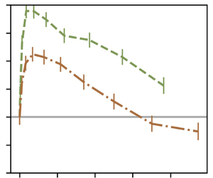
Figure 5 shows the normalised velocity difference  $\Delta V/u'$ against particle diameter. All the measurements were taken at the same location, at the centreline of the wind tunnel. All the curves show the same trend: the settling velocity is enhanced for small particles, and this enhancement reaches a maximum,
  $max(\Delta V /u')$. After the maximum, the settling velocity enhancement decreases until it reaches a point where it is negative, that is, particle settling is hindered by turbulence. For very large particles (not attainable with our injection system),
  $\Delta V /u'$ would eventually become zero as they follow ballistic trajectories, unimpeded by turbulence. A discussion on the mechanisms that control enhancement and hindering of the settling velocity is available in § 5.

Figure 5. Particle velocity over the carrier phase fluctuations  $\Delta V/u' = (\langle V \rangle _{d_p} - V_{\beta } - V_{physical} - V_T)/u'$ against the particle's diameter
  $d_p$ for a volume fraction of
  $0.5\times 10^{-5}$ (a),
  $1.0\times 10^{-5}$ (b) and
  $2.0\times 10^{-5}$ (c). The data from the AG are in solid lines, the OG in dashed line and the RG in dash–dotted lines. The error bars show the estimation of the error in the velocity measurements induced by the determination of the misalignment angle. A darker colour corresponds to a higher mean velocity
  $U_\infty$.
Particle settling velocity tends to depend on the turbulence characteristics, that is, in this study, it depends on the type of grid used in the experiments. Series taken with the OG configuration show a higher enhancement for all volumes fractions (green dashed line). On the contrary, AG turbulence (in blue solid lines) causes mostly hindered settling, with enhancement present only for a small range of diameters. Finally, measurements taken with the RG (red dash–dotted lines) show an intermediate behaviour between the two other grid configurations.
A combination between the Rouse and Stokes numbers,  $Ro\,St$, has already been proven to be an interesting scaling (Ghosh et al. Reference Ghosh, Davila, Hunt, Srdic, Fernando and Jonas2005), as it was shown in several studies to collapse the data better (Good et al. Reference Good, Ireland, Bewley, Bodenschatz, Collins and Warhaft2014; Petersen et al. Reference Petersen, Baker and Coletti2019; Mora et al. Reference Mora, Obligado, Aliseda and Cartellier2021; Yang & Shy Reference Yang and Shy2021). The Rouse–Stokes number can be expressed as a ratio between a characteristic length of the particle
  $L_p$ and a characteristic length of the flow. Here
  $L_p$ can be seen as the distance that a particle will travel to adjust its velocity to the surrounding fluid starting with a velocity
  $V_T$. Using the Kolmogorov time scale in the Stokes number and
  $u'$ in the Rouse number, the Taylor microscale appears to be the characteristic length scale of the flow:
 \begin{equation} Ro\,St = \frac{\tau_p}{\tau_\eta}\frac{V_T}{u'} = \sqrt{15} \frac{V_T \tau_p}{\lambda} = \sqrt{15} \frac{L_p}{\lambda} \quad \text{with} \, L_p = V_T\tau_p \, \text{as} \, \lambda = \sqrt{15}\tau_\eta u'. \end{equation}
 In figure 6, we present  $\Delta V/u'$ against the Rouse–Stokes number
  $Ro\,St$. Similar to figure 5, each panel presents data from a different value of volume fraction.

Figure 6. Enhancement of the particle velocity, normalised by the turbulent r.m.s. velocity,  $\Delta V/u'$, against the Rouse–Stokes number: (a)
  $\phi =0.5\times 10^{-5}$; (b)
  $\phi =1.0\times 10^{-5}$; and (c)
  $\phi =2.0\times 10^{-5}$. Lines follow the legend of figure 5.
The  $Ro\,St$ number gives a better collapse of the position of maximum of enhancement than the Rouse number or Stokes number alone. Figure 6 indicates that enhancement of the settling velocity reaches a maximum for a Rouse–Stokes number around 0.6, which is consistent with previous findings. Yang & Shy (Reference Yang and Shy2021) reported a maximum for a
  $Ro\,St$ around 0.72–1 in a Taylor–Couette flow, whereas Petersen et al. (Reference Petersen, Baker and Coletti2019) presented a maximum of enhancement for
  $Ro\,St$ of order 0.1. Alternative scalings have been tested on our data, with the results provided for completion in Appendix A. These measurements reveal that, for a fixed
  $Re_\lambda$, the enhancement increases with volume fraction, consistent with Aliseda et al. (Reference Aliseda, Cartellier, Hainaux and Lasheras2002) and Monchaux & Dejoan (Reference Monchaux and Dejoan2017).
We observe that the enhancement is much stronger for the low values of  $Re_\lambda$ (
 $\in [30\unicode{x2013}70]$, OG and RG) than for the higher
  $Re_\lambda$ (
 $\in [260\unicode{x2013}520]$, AG) for all volume fractions. As shown in figure 2(a), the settling enhancement decreases significantly with an increase in the flow Taylor–Reynolds number, with Taylor–Reynolds number significantly higher for the AG turbulence than for the two other grids
  $Re_{\lambda AG} \gg Re_{\lambda RG} > Re_{\lambda OG}$. However, we observe when the Taylor–Reynolds number is varied by increasing the inlet velocity
  $U_\infty$ alone, while keeping the same grid turbulence generation system, the trend is reversed: the settling enhancement increases with an increase in
  $Re_\lambda$ within the small range achieved with each grid, and keeping a quasiconstant large-to-small scales ratio. Thus, settling enhancement depends strongly on the characteristics of the turbulence, as reported in Mora et al. (Reference Mora, Obligado, Aliseda and Cartellier2021). While the study of Mora et al. (Reference Mora, Obligado, Aliseda and Cartellier2021) obtained the same trend by comparing with data from the literature, in this study the entire range of Reynolds number and turbulent length scales were explored in the same facility.
This would suggest that the maximum of enhancement has a non-monotonic behaviour with the turbulent Reynolds number, as reported in Mora et al. (Reference Mora, Obligado, Aliseda and Cartellier2021). A non-monotonic dependency of the degree of enhancement with Reynolds number has also been observed recently in Yang & Shy (Reference Yang and Shy2021). This effect of  $Re_\lambda$ on the maximum of enhancement confirms that the settling velocity modification is a multiscale phenomenon and one turbulent scale is not sufficient to characterise it (Tom & Bragg Reference Tom and Bragg2019).
Although  $u'$ has been widely used in the literature to normalise
  $\Delta V$, it has already been pointed out that there is no consensus on the scale for settling modification (Tom & Bragg Reference Tom and Bragg2019). The influence of the Reynolds number on the settling modification is also affected by normalising
  $\Delta V$ with
  $u'$. Since the range of flow scales that interact with the particles depends on the Stokes number, an interesting choice would be to non-dimensionalise
  $\Delta V$ with a vertical velocity that depends on
  $St$. Similarly to previous studies (Good et al. Reference Good, Ireland, Bewley, Bodenschatz, Collins and Warhaft2014; Rosa et al. Reference Rosa, Parishani, Ayala and Wang2016), a normalisation of the results with the terminal velocity
  $V_T = St g \tau _\eta$ is proposed in figure 7. Figure 7 uses the same legend as figures 5 and 6. Normalising with
  $V_T$, the three different sets of curves for the three turbulence generation schemes are observed to collapse in figure 6. However, looking closely at figure 7, the Reynolds number dependency of the settling velocity modification is still non-monotonic, even after normalising with a velocity scale different than
  $u'$.
$u'$.

Figure 7. Enhancement of the particle velocity, normalised by the particle terminal velocity,  $\Delta V/V_T$, against the Rouse–Stokes number: (a)
  $\phi =0.5\times 10^{-5}$; (b)
  $\phi =1.0\times 10^{-5}$; and (c)
  $\phi =2.0\times 10^{-5}$. Lines follow the legend of figure 5.
3.4. Variance of the vertical particle velocity
The variance of the vertical particle velocity  $\langle (v'_y)^2 \rangle$ normalised by the Kolmogorov velocity square is shown in figure 8. In figure 8(a), we observe that the variance increases with the Reynolds number
  $Re_\lambda$. This is expected since the fluid velocity variance increases with the Reynolds number and so does the particle velocity variance. The normalised particle velocity variance was also computed for each bin of diameters to have the influence of the Stokes number and the Rouse number on this metric. Figure 8(b) shows that the variance decreases slowly with the Rouse–Stokes number. This is consistent with the fact that the filtering by inertial particles becomes more important as inertia increases. Inertial particles with higher Stokes number are less sensitive to the carrier flow's high velocity fluctuations.

Figure 8. Variance of the vertical particle velocity  $\langle (v'_y)^2 \rangle$ normalised by the Kolmogorov velocity square
  $u_\eta ^2$. The variance is plotted towards the Reynolds number
  $Re_\lambda$ in (a) and towards the Stokes number in (b). The symbols follow the legend of figure 4.
3.5. Scaling of the maximum of enhancement
As no theoretical consensus have been found on the settling velocity modification, empirical scalings are proposed. This study focuses on the value and location of maximum of enhancement  $max(\Delta V/u')$, and not on the critical
  $Ro\,St$, where enhancement turns into hindering, as most cases with the passive grid did not reach the transition enhancement/hindering for high Rouse number, contrary to Mora et al. (Reference Mora, Obligado, Aliseda and Cartellier2021). As said in the previous section, the enhancement seems to increase when varying only the wind tunnel velocity
  $U_\infty$. In order to take this trend into account, a global Reynolds number is introduced,
  $Re_G = M U_\infty /\nu$, based on
  $U_\infty$ and
  $M$ the mesh spacing in the turbulence-generating grid. Several dimensionless parameters were tested to scale
  $max(\Delta V/u')$: the global Reynolds number
  $Re_G$, the volume fraction
  $\phi _v$, the Taylor-scale Reynolds number
  $Re_\lambda$, a Reynolds number based on the integral length scale, and the
  $Ro$ or
  $St$ numbers corresponding to the maximum of enhancement. The best scaling from the parameters above was found to be a combination of
  $Re_\lambda$,
  $Re_G$ and
  $\phi _v$.
Figure 9(a) represents  $max(\Delta V/u')$ against
  $Re_\lambda ^\alpha \phi _v^\beta Re_G^\gamma$, where
  $\alpha$,
  $\beta$ and
  $\gamma$ are best-fit exponents:
 \begin{equation} max(\Delta V/u') \sim Re_\lambda^\alpha \phi_v^\beta Re_G^\gamma, \end{equation}
with  $\alpha = -1.1$,
  $\beta = 0.6$ and
  $\gamma = 0.9$. The values of
  $\alpha$,
  $\beta$ and
  $\gamma$ are consistent with previous observations: the maximum of enhancement increases with inlet velocity and volume fraction but decreases with an overall increase of
  $Re_\lambda$ (when varying the Reynolds number on the entire range [30, 520]).

Figure 9. Scaling of the settling velocity with  $Re_\lambda$,
  $Re_G$ and
  $\phi _v$: (a)
  $max(\Delta V/u')$ versus
  $Re_\lambda ^\alpha \phi _v^\beta Re_G^\gamma$ with the fitted value of
  $\alpha$,
  $\beta$ and
  $\gamma$; (b)
  $max(\Delta V/u')$ divided by the scaling versus the Rouse–Stokes number.
Figure 9 shows figure 6(c) with  $\Delta V/u'$ divided by the power law scaling. A gap in data exists due to the jump in Reynolds number between the AG and the two passive grids (see figure 2). No measurements were taken for
  $Re_\lambda$ between 70 and 260, since the present experimental set-up cannot reach those intermediate values.
Figure 9 shows that no simple scaling of the peak of settling enhancement can be inferred from this data. The dispersion of the results is partly due to the effect of the different large-scale turbulence, as discussed in the next section.
4. Influence of large-scale structures
Although the OG and RG create very similar values of turbulent intensity, the settling speed of inertial particles in these two flows are very different. Indeed, RG data (dash–dotted lines) is as different from OG data as it is from AG data (see figures 5 and 6). This discrepancy between RG and OG behaviours can be explained by the difference in integral length scales between these two turbulent flows (see table 1 and figure 2).
Figure 10 illustrates the settling velocity modification from two series with similar Reynolds numbers, turbulent intensities and volume fractions, but different integral length scales  $\mathcal {L}_{a0}$. The figure is plotted against
  $Ro\,St$ but presents a similar trend when made with
  $Ro$ or
  $St$. It can be seen that the degree of settling enhancement is stronger for a smaller integral length scale and this behaviour is consistent for different volume fractions and wind tunnel Reynolds numbers. This suggests that the integral length scale and large-scale structures play a role in the settling velocity modification. According to the study of Tom & Bragg (Reference Tom and Bragg2019), there is a length scale
  $l_c(St)$ above which the effects of particle inertia are negligible and only the flow scales smaller than
  $l_c$ contribute to the settling velocity enhancement. Here
  $l_c$ has been proposed to be an increasing function of the Stokes number, thus, as
  $St$ increases, the range of flow scales impacting the settling velocity becomes larger. Consequently, we would expect the integral length scale to play a role on
  $\Delta V/u'$ only when the Stokes number is above
  $St(l_c)$. With our experiments, we provide the first evidence of settling velocity modification by turbulence where the integral length scale is the only difference between two turbulent datasets, in figure 10. According to the
  $l_c$ hypothesis, one would expect the curves from the RG and the OG to collapse for the
  $St < St(l_c)$ data. Figure 10 reveals that the integral length scale has a measurable influence on the settling velocity modification for almost the entire range of
  $Ro\,St$ number studied, and not only for the large
  $Ro\,St$. The data presented in figure 10 shows a collapse for
  $Ro\,St < 0.1$, suggesting that the integral length scale does not play a role in settling velocity modification for very small
  $Ro\,St$. This contradicts the hypothesis in Tom & Bragg (Reference Tom and Bragg2019), unless
  $l_c < \mathcal {L}$ for the smallest particles in the flow. However, Tom & Bragg (Reference Tom and Bragg2019) showed that
  $l_c(St)$ is larger than expected and can be larger than the flow integral scale even for
  $St=O(0.1)$.

Figure 10. The OG and RG data. Settling velocity difference over the carrier-phase fluctuations  $(\Delta V)/u'$ against the Rouse–Stokes number, for a volume fraction of
  $2.0\times 10^{-5}$. Panel (a) displays data taken with an inlet velocity of
  $2.7\ {\rm m}\ {\rm s}^{-1}$, whereas the bulk velocity in (b) is
  $5.0\ {\rm m}\ {\rm s}^{-1}$.
As a consequence of the evidence provided in this paper, the preferential sweeping mechanism is more accurate at explaining the observations in flows where the large-scale structures are reduced in size.
5. Mechanisms of the settling velocity modification
5.1. Competition between preferential sweeping and loitering
The different models of the settling velocity modification require the measurement of fluid variables (flow structure, slip velocity, etc.) that is not possible, at least in an instantaneous manner, in large Reynolds number two-phase flows. Nevertheless, qualitative comparison of our experimental data with theoretical models for the proposed mechanisms shows good agreement. The enhancement of the settling velocity for small Stokes number, i.e. small diameter, particles found in our experiments is consistent with the preferential sweeping mechanism (Maxey Reference Maxey1987). The hindering for large Stokes number found at high Reynolds numbers, on the other hand, is consistent with the loitering mechanism proposed by Nielsen (Reference Nielsen1993). The mechanisms and the parameters that control the transition between enhancement and hindering, for which this manuscript provides novel data at turbulent Reynolds numbers and length scales not studied before, remain poorly understood and needs theoretical analysis.
Indeed, the  $Ro$,
$Ro$,  $St$ or
  $Ro\,St$ critic that set the transition between enhancement and hindering have a non-monotonic dependence with the Reynolds number. No simple scaling of the Stokes or Rouse critic could be found from other non-dimensional parameters (i.e. volume fraction, global Reynolds number or Taylor-based Reynolds). However, the fact that the maximum of enhancement collapses for
  $Ro\,St \approx 0.6\unicode{x2013}1.0$ gives a threshold for which the loitering effect starts to balance out the preferential sweeping mechanism (although enhancement remains the main outcome).
As mentioned before, the  $Ro\,St$ number can be expressed as the ratio between
  $L_p$ and
  $\lambda$, where
  $L_p$ is the distance that a particle will travel to adjust its velocity to the surrounding fluid starting with a velocity
  $V_T$. Furthermore, the Taylor microscale can be seen as the separation between two large-scale eddies (Mazellier & Vassilicos Reference Mazellier and Vassilicos2008). When
  $L_p$ starts to be larger than
  $\lambda$ the preferential sweeping mechanism becomes less and less important since particles take a longer time and distance to respond to the fluid. As particles are less often swept in the downward side of eddies with an increase in
  $L_p$ they cross both upward and downward regions of the flow which result in a more frequent loitering. Consistently, figure 10 shows that the preferential sweeping mechanism is more effective when the flow's large-scale structures are smaller.
5.2. Collective effects
Numerous studies have shown an increase in the particle settling velocity with the particle local concentration (Aliseda et al. Reference Aliseda, Cartellier, Hainaux and Lasheras2002; Monchaux & Dejoan Reference Monchaux and Dejoan2017; Huck et al. Reference Huck, Bateson, Volk, Cartellier, Bourgoin and Aliseda2018). An estimate of the particle local concentration can be obtained with the use of Voronoï tessellations (Monchaux, Bourgoin & Cartellier Reference Monchaux, Bourgoin and Cartellier2010). In this study, only one-dimensional statistics of a 3-D flow are collected with the PDPA. For such signals, special attention is required as the analysis of preferential concentration via Voronoï tessellations has shown to present some bias (Mora et al. Reference Mora, Aliseda, Cartellier and Obligado2019a). A Voronoï cell is defined as the portion of the temporal signal closer to one particle than to any other ones. The inverse of the Voronoï cell length  $L$ gives an indication of the particle local concentration
  $C=1/L$. Preferential concentration is observed when small and large Voronoï cells are over represented compared with a random Poisson process (RPP). In other words, the probability distribution function (PDF) of the normalised Voronoï cell length
  $\mathcal {V}=L/\langle L \rangle$ crosses the PDF of a RPP twice. Before the first crossing, small Voronoï cells are over represented showing the presence of over populated regions, or clusters. Similarly, after the second crossing large Voronoï cells are more probable than for a RPP showing the presence of depleted regions (i.e. voids). Clusters and voids are defined as a group of connected cells with cell length smaller than the first, respectively larger than the second, crossing with the PDF of a RPP. According to Mora et al. (Reference Mora, Aliseda, Cartellier and Obligado2019a), clustering can be present and not be detected by the use of one-dimensional Voronoï tessellations. However, if the standard deviation of the normalised cell length
  $\sigma _\nu$ is larger than for a RPP distribution
  $\sigma _\nu > \sigma _{RPP}$, it is a reliable evidence of the presence of preferential concentration. For the next, we will only consider cases for which
  $\sigma _\nu / \sigma _{RPP} > 1.2$ to avoid time series that present a lack of information.
Figure 11(c) shows the conditional particle velocity on the local concentration compared with the average settling velocity over all particles  $\langle v_y(t) \rangle$ versus the normalised concentration
  $C/C_0 = 1/\mathcal {V}$. In agreement with previous studies (Huck et al. Reference Huck, Bateson, Volk, Cartellier, Bourgoin and Aliseda2018), the settling velocity is constant or increased with the particle local concentration.

Figure 11. Mean settling velocity of particles in clusters  $\langle v_y \rangle _{clusters}$ (a) and particles in voids
  $\langle v_y \rangle _{voids}$ (b) normalised by the unconditional average
  $\langle v_y \rangle$. Panel (c) shows the settling velocity conditioned on the particle local concentration
  $\langle v_y \rangle |_{C/C_0}$ normalised by the r.m.s. of the carrier phase fluid fluctuations. Symbols and lines follow the legend of figure 4.
The mean settling velocity for particles in clusters and particles in voids are shown in figures 11(a) and 11(b). For low Reynolds number, the settling velocity for particles in clusters is, for most cases, larger than the global settling while particles in voids settle slower than the unconditional average. Figure 11 shows that the particle local concentration and collective effects have an influence on the settling rate in our dataset as previously observed in Aliseda et al. (Reference Aliseda, Cartellier, Hainaux and Lasheras2002), Huck et al. (Reference Huck, Bateson, Volk, Cartellier, Bourgoin and Aliseda2018) and Petersen et al. (Reference Petersen, Baker and Coletti2019).
5.3. Sweep-stick mechanism
The sweep-stick mechanism proposed by Chen, Goto & Vassilicos (Reference Chen, Goto and Vassilicos2006), Goto & Vassilicos (Reference Goto and Vassilicos2008) and Coleman & Vassilicos (Reference Coleman and Vassilicos2009) states that there is a strong correlation between the carrier flow zero-acceleration points and inertial particle positions. This mechanism was first proposed to explain the preferential concentration of inertial particles for direct numerical simulation data with zero gravity. The modified sweep-stick mechanism (Falkinhoff et al. Reference Falkinhoff, Obligado, Bourgoin and Mininni2020) suggests that, in the presence of gravity, particles stick to low, but non-zero, acceleration points. Zero-acceleration points were shown to have an average lifetime of  $\tau _\mathcal {L}$ with
  $\tau _\mathcal {L}=\mathcal {L}/u'$ the flow integral time scale (Coleman & Vassilicos Reference Coleman and Vassilicos2009). This mechanism is restricted to cases where the particle relaxation time is much smaller than the zero acceleration points life-time, that is to say when
  $\tau _p \ll \tau _\mathcal {L}$ or
  $St_\mathcal {L} = \tau _p/\tau _\mathcal {L} \ll 1$ and for
  $St > 1$.
The average acceleration of the fluid at the particle's position can be estimated from the ensemble average of the Maxey–Riley equation,
 \begin{equation} \frac{\langle v_y^p(t) \rangle}{V_T} = \frac{\langle u_y(\boldsymbol{x}^p(t),t) \rangle}{V_T} + 1. \end{equation}
Similarly as in Falkinhoff et al. (Reference Falkinhoff, Obligado, Bourgoin and Mininni2020), we use the approximation that  $\langle a_y(\boldsymbol {x}^p(t),t) \rangle \sim \langle u_y(\boldsymbol {x}^p(t),t) \rangle / \tau _\mathcal {L}$ with
  $a_y(\boldsymbol {x}^p(t),t)$ the fluid acceleration at the particle position. The term
  $\langle u_y(\boldsymbol {x}^p(t),t) \rangle /V_T$ can be rewritten as
  $\langle a_y(\boldsymbol {x}^p(t),t) \rangle / (gSt_\mathcal {L})$ with
  $St_\mathcal {L} = \tau _p/\tau _\mathcal {L}$, as follows:
 \begin{equation} \frac{\langle a_y(\boldsymbol{x}^p(t),t) \rangle}{ gSt_\mathcal{L}} =\frac{\langle v_y^p(t) \rangle}{V_T} - 1. \end{equation}
Then with the fact that  $\tau _\mathcal {L} = \mathcal {L}/u'$ and
  $St_\mathcal {L}/St=\tau _\eta u'/\mathcal {L}$ we get
 \begin{equation} \frac{\langle a_y(\boldsymbol{x}^p(t),t) \rangle}{gSt} = (\tau_\eta u'/\mathcal{L})\left(\frac{\langle v_y^p(t) \rangle}{V_T} - 1 \right). \end{equation}
 To be able to compare with the data from Falkinhoff et al. (Reference Falkinhoff, Obligado, Bourgoin and Mininni2020) for which the vertical axes is directed in the opposite direction, we plot the quantity  $(\tau _\eta u'/\mathcal {L})(1 - \langle v_y^p(t) \rangle /V_T)$ in figure 12. This quantity is positive when there is hindering (
 $\langle v_y^p(t) \rangle < V_T$) and negative in the case of enhancement (
 $\langle v_y^p(t) \rangle > V_T$).

Figure 12. Average normalised acceleration of the fluid elements  $\langle a_y(\boldsymbol {x}^p(t),t) \rangle /(gSt)$ following (5.3) as a function of the corrected settling velocity normalised by the terminal velocity
  $(\langle V \rangle _{d_p} - V_{\beta } - V_{physical})/V_T$. The black triangles present the data from the study of Falkinhoff et al. (Reference Falkinhoff, Obligado, Bourgoin and Mininni2020). The data from the present study, taken with the AG and a volume fraction of
  $0.5\times 10^{-5}$, are shown in blue.
Figure 12 presents the estimation of the normalised fluid acceleration at the particles’ position for the AG data. The data from the direct numerical simulation of Falkinhoff et al. (Reference Falkinhoff, Obligado, Bourgoin and Mininni2020), also shown in figure 12, correspond to a turbulent flow Reynolds number of  $Re_\lambda \approx 300$, various Stokes numbers and Froude number (
 $St = 1, 3, 6, 8, 9$), and Froude numbers (
 $Fr = (\varepsilon ^3 / \nu )^{1/4}1/g = 0.15, 0.23, 0.45, 1.36$). As for the experimental data where the fluid velocity at the particle position is not accessible, we can only compare the value of the acceleration of the fluid elements between the experiments and the simulation. To better compare with the numerical simulation, only samples taken with the AG and with a
  $St$ number close to 1, 3, 6, 8, 9 are presented in figure 12. There is a reasonable agreement in the value of
  $\langle a_y(\boldsymbol {x}^p(t),t) \rangle /(gSt_\mathcal {L})$ between both studies. The slope of the data is controlled by the value of
  $\tau _\eta u'/\mathcal {L}$, and thus depends only upon the flow characteristics. Discrepancies can be found between the values from the numerical simulation and the experiment since the Froude number and the flow integral length scale are different.
6. Conclusion
The settling velocity of sub-Kolmogorov inertial particles in wind tunnel decaying turbulence is presented and analysed. Accurate settling velocity measurements were carefully collected and calibrated, by correcting different experimental sources of potential bias. First, a correction for the PDPA misalignment angle is computed and applied. Second, secondary flows in the wind tunnel test section were characterised,  $V_{physical}$, for both single-phase and two-phase flows. High resolution in the vertical velocity, compared with Mora et al. (Reference Mora, Obligado, Aliseda and Cartellier2021), was obtained thanks to a new PDPA set-up. This, together with the detailed measurements of alignment and secondary motions, created a more accurate dataset of settling velocity for small Stokes number particles.
The results in this study confirm and extend the trends observed previously (among others by Wang & Maxey (Reference Wang and Maxey1993), Aliseda et al. (Reference Aliseda, Cartellier, Hainaux and Lasheras2002), Good et al. (Reference Good, Ireland, Bewley, Bodenschatz, Collins and Warhaft2014) and Mora et al. (Reference Mora, Obligado, Aliseda and Cartellier2021)). Specifically, the settling velocity enhancement, that has been observed under a wide range of conditions, disappears with an increase of global (wind tunnel) Reynolds number, and turns to hindering at high Reynolds numbers  $Re_\lambda > 260$. This dependence with Reynolds number is in contradiction with most numerical studies (Bec et al. Reference Bec, Homann and Ray2014; Rosa et al. Reference Rosa, Parishani, Ayala and Wang2016; Tom & Bragg Reference Tom and Bragg2019). However, for a smaller range of Reynolds numbers, the maximum of enhancement is proportional to the inlet velocity
  $U_\infty$, and therefore to the global Reynolds number. A new phenomenological scaling considering the influence of the bulk velocity has been proposed.
The range of volume fractions investigated is limited, and precludes the influence of this variable on settling enhancement from appearing. Different turbulence generation schemes allow for flows with different integral and Taylor length scales, at the same turbulent intensities and Reynolds numbers. We show that even if the Reynolds number and the turbulent intensity are similar, significant differences in the settling modification remain, due to widely different integral length scales. This suggests an important role of the large flow structures on the settling velocity modification.
The settling rate modification observed in this study is due to the intervention of several mechanisms, including at least preferential sweeping, loitering and sweep-stick mechanisms, operating on different ranges of Stokes and Rouse numbers. In addition to the aforementioned mechanisms, our results show that collective effects might take a part in the settling velocity modification.
Acknowledgements
We also would like to thank L. Vignal for her help with the PDPA measurements and V. Govart for producing experimental rigs.
Funding
This work has been supported by a LabEx Tec21 grant (Investissements d'Avenir – grant agreement no. ANR-11-LABX-0030).
Declaration of interest
The authors report no conflict of interest.
Appendix A. Additional scalings
Particle settling velocity is often presented against the Stokes number (Wang & Maxey Reference Wang and Maxey1993; Yang & Lei Reference Yang and Lei1998; Aliseda et al. Reference Aliseda, Cartellier, Hainaux and Lasheras2002; Good et al. Reference Good, Ireland, Bewley, Bodenschatz, Collins and Warhaft2014; Rosa et al. Reference Rosa, Parishani, Ayala and Wang2016; Petersen et al. Reference Petersen, Baker and Coletti2019; Yang & Shy Reference Yang and Shy2021), the Rouse number (Good et al. Reference Good, Gerashchenko and Warhaft2012, Reference Good, Ireland, Bewley, Bodenschatz, Collins and Warhaft2014; Mora et al. Reference Mora, Obligado, Aliseda and Cartellier2021) and a Rouse number based on the Kolmogorov scale  $V_T/u_\eta$ (Good et al. Reference Good, Ireland, Bewley, Bodenschatz, Collins and Warhaft2014). Figure 13 shows the present data against these three different parameters.

Figure 13. Particle velocity over the carrier phase fluctuations  $\Delta V/u'$ against the Stokes number (a), Rouse number (b) and the Rouse number based on the Kolmogorov scale (c) for a volume fraction of
  $2.0\times 10^{-5}$. Line styles follow the caption of figure 5.
Appendix B. Stationarity of the temporal signal and PDF of particles’ velocities
In this section we show the raw velocity obtained with the PDPA. The temporal signals are stationary (see figure 14). In this figure, one portion of the time signals is presented for each of the three grids using a volume fraction of  $\phi _v = 1.0 \times 10^{-5}$ and an inlet velocity of
  $U_\infty \approx 4.0\ {\rm m}\ {\rm s}^{-1}$. Figure 14(a) corresponds to the streamwise velocity whereas figure 14(b) represents the vertical velocity.

Figure 14. Temporal signals of the streamwise (a) and the vertical velocity (b). One example of temporal PDPA signal is shown for each of the three grids: AG in blue; OG in green; and RG in brown. The measurements were taken for a volume fraction of  $\phi _v = 1.0 \times 10^{-5}$ and an inlet velocity
  $U_\infty \approx 4.0\ {\rm m}\ {\rm s}^{-1}$.
It can also be observed that all inertial particles horizontal and vertical velocities have a Gaussian distribution (see figure 15). The skewness ( $\mu _3/\mu _2^{3/2}$) and the kurtosis (
 $\mu _4/\mu _2^{2}$) have been computed for each velocity distribution (with
  $\mu _n$ the
  $n$th central moment). The average values over all these experiments for both of these moments are
 \begin{align} \frac{\mu_3}{\mu_2^{3/2}} (V_x) =-0.12, \quad \frac{\mu_4}{\mu_2^{2}} (V_x) = 3.00, \quad \frac{\mu_3}{\mu_2^{3/2}} (V_y) = 0.08 \quad \text{and} \quad \frac{\mu_4}{\mu_2^{2}}(V_y) = 3.17 . \end{align}
Figure 15. The PDF of the streamwise (a,c,e) and vertical (b,d,f) velocity for each type of grid: AG (a,b); OG (c,d); and RG (e,f).
In figure 16 the skewness and the kurtosis for each velocity PDF is shown against the mean streamwise velocity  $U_\infty$. Since the skewness always falls between
  $-$0.5 and 0.5, the velocity distributions are considered symmetrical. The values of the flatness are also relatively close to 3, the value of the Gaussian distribution.

Figure 16. Skewness (a,b) and kurtosis (c,d) of the velocity PDF against the mean streamwise velocity  $U_\infty$. Panels (a,c) show the moments for the horizontal velocity whereas (b,d) correspond to the vertical velocity. The different symbols (
 $\blacksquare$), (
 $\bullet$) and (
 $\blacklozenge$) represent the RG, AG and OG, respectively. The size of the symbol is proportional to the volume fraction and darker colours correspond to higher mean velocities. The quantity given in each panel is the mean value over all the conditions.
Appendix C. Determination of the PDPA misalignment angle
A small deviation angle between the PDPA axes and the wind tunnel axes is always present even if the best precautions were taken during the set up of the device. The deviation angle has a negligible impact on the horizontal velocity but can induce a significant bias on the measurements of the settling velocity, since the particle's horizontal velocity component is much larger than the vertical one.
We call  $\beta$ the angle between the axes of the PDPA and the axes of the wind tunnel. Here
  $V_{XPDPA}$ and
  $V_{YPDPA}$ are, respectively, the streamwise and vertical components of the velocity measured by the instrument while
  $V_{XWT}$ and
  $V_{YWT}$ are the exact particle velocity components in the wind tunnel coordinate system (see Mora et al. Reference Mora, Obligado, Aliseda and Cartellier2021).
By projecting the accurate droplet velocity in the frame of reference of the PDPA we get
 \begin{equation}
\overrightarrow{V_{YWT}} =
\begin{pmatrix}\underbrace{V_{YPDPA}\cos(\beta)}_{{\approx} V_{YPDPA}} - V_{XPDPA}\sin(\beta)\end{pmatrix}\overrightarrow{y}.
\end{equation}
\begin{equation}
\overrightarrow{V_{YWT}} =
\begin{pmatrix}\underbrace{V_{YPDPA}\cos(\beta)}_{{\approx} V_{YPDPA}} - V_{XPDPA}\sin(\beta)\end{pmatrix}\overrightarrow{y}.
\end{equation}
Since the PDPA was set in non-coincident mode, we do not have access to the horizontal component  $V_{XPDPA}$ corresponding to the biased settling velocity. We then approximate by using the mean of the time series horizontal velocity
  $V_{XPDPA} \approx \langle U \rangle$ and define the angle-corrected velocity as follows:
 \begin{equation} V_{YWT} = V_{YPDPA} - \underbrace{ \langle U \rangle \sin(\beta)}_{V_{\beta}}.\end{equation}
In order to compute the vertical velocity due to the horizontal component projection  $V_\beta$, we estimated the misalignment angle
  $\beta$ through measurements of olive oil droplets settling velocities. We used olive oil to be closer to the limit of very small diameter and very small volume fraction
  $\phi _v$. Indeed, olive oil droplets have a much smaller average diameter,
  $\langle d_p \rangle \approx 3\ \mathrm {\mu }{\rm m}$, and a less polydispersed size distribution than water droplets.
The settling velocity of olive oil droplets were collected for different free stream velocities in the absence of a grid in order to have a flow as laminar as possible. Measurements were taken when the probe volume was situated on the centre, close to the wall of the wind tunnel and each time the PDPA had to be realigned. The particle speed in a still fluid is computed from the particle relaxation time  $\tau _p$ including the nonlinear drag from the Schiller–Naumann semiempirical equation (Clift et al. Reference Clift, Grace and Weber1978):
 \begin{equation} V_T = \tau_p g \quad \text{with} \ \tau_p = \frac{\rho_p d_p^2}{18\mu_f(1+0.15Re_p^{0.687})}, \end{equation}
where  $\mu _f$ is the air dynamic viscosity,
  $g$ the gravitational acceleration,
  $d_p$ the particles’ diameter, the oil droplet density
  $\rho _p = 900\ {\rm kg}~{\rm m}^{-3}$ and
  $Re_p = V_T d_p/\nu$ the particle Reynolds number. As the diameter of olive oil droplets is extremely small the actual velocity is supposed to be equal to the Stokes velocity
  $V_{YWT} = V_T$. We then get from (C2) that
 \begin{equation} \langle V_{YPDPA} \rangle = V_T + \langle U \rangle \sin (\beta). \end{equation}
 With several free stream velocities and (C4) a least-squares polynomial fit on the values of  $\langle V_{YPDPA} \rangle$ and
  $\langle U \rangle$ can be performed to estimate
  $\sin (\beta )$. Figure 17 shows
  $\langle V_{YPDPA} \rangle$ against
  $\langle U \rangle$ for the probe volume on the centre where a linear fit was done and the slope gives the value of
  $\sin (\beta )$. In our case,
  $\beta$ is found equal to
  $\beta = 1.5^\circ \pm 0.3^\circ$.

Figure 17. Here  $\langle V_{YPDI} \rangle$ against
  $\langle U \rangle$ for the different incoming velocities with olive oil droplets measurements. A linear fit of the data is shown in dashed line.


 Open access