


1. Introduction
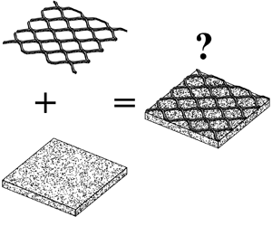
Flow over porous walls comprises an extensive number of natural phenomena, ranging from blood vessels to the atmospheric boundary layer (ABL) developing over a forest canopy. The latter can be considered as a turbulent boundary layer (TBL) developing over a porous wall. An example of porous walls, constructed from packed spheres, is shown in figure 1. Here, both walls approximately have the same permeability (i.e. the inverse of resistance of a substrate to fluid flows) and some form of roughness: the wall shown in figure 1(a) has roughness protrusions (positive skewness) above the porous wall, while in figure 1(b) this roughness interface comprises recesses (negative skewness). Thus, a realistic representation of a porous wall is both permeable and rough to some extent, and the effects of both permeability and roughness have to be considered for characterisation of a TBL developing over such wall.

Figure 1. Illustrations of realistic permeable walls with roughness interfaces: (a) positive and (b) negative skewnesses. Adapted from Rosti, Cortelezzi & Quadrio (Reference Rosti, Cortelezzi and Quadrio2015).
1.1. Rough walls
The presence of rough walls increases skin friction from that of smooth walls and thus the time-averaged streamwise velocity of TBLs developing over rough walls ( $U_r^+$, subscript ‘
 $r$’ denotes a rough wall; y, wall-normal location) can be written as a downward shift of the logarithmic region from the smooth wall velocity profile:
 \begin{equation} U_r^+= \frac{1}{\kappa} \ln \left[ \frac{(y + d) U_{\tau}}{\nu} \right] + B - \Delta U_r^+= \frac{1}{\kappa} \ln (y + d)^++ B - \Delta U_r^+ .\end{equation}
The viscous-scaled velocity is defined as  $U_r^+ \equiv U_r/U_{\tau }$, where
  $U_{\tau } \equiv \sqrt {\tau _w/\rho }$ is the friction velocity,
  $\tau _w$ and
  $\rho$ are the wall shear stress (WSS) and the density of fluid, respectively. The logarithmic profile is defined as follows:
  $\kappa$ is the von Kármán constant,
  $d$ is the zero-plane displacement,
  $\nu$ is the kinematic viscosity of fluid, and
  $B$ is the log-law intercept. In the fully rough regime, the logarithmic shift
  $\Delta U_r^+$, also known as the Hama roughness function (Hama Reference Hama1954), is defined as
 \begin{equation} \Delta U_r^+= \frac{1}{\kappa} \ln \left(\frac{k_{s_r} U_{\tau}}{\nu}\right) + B - B_{FR} = \frac{1}{\kappa} \ln k_{s_r}^++ B - B_{FR} ,\end{equation}
where  $k_{s_r}$ is the equivalent sand grain roughness of a rough wall (note that we use different subscripts throughout this study to distinguish the equivalent sand grain roughness between different test surfaces: subscripts ‘
 $r$’ for rough, ‘
 $p$’ for porous, and ‘
 $pr$’ for porous–rough walls) and
  $B_{FR} = 8.5$ is the ‘fully’ rough intercept of the velocity profile of sand grain roughness. It should be noted that the ‘equivalent sand grain roughness’ is a measure of roughness effect on the flow relative to that of a uniform sand grain roughness (Nikuradse Reference Nikuradse1933); it can only be determined by flow measurements. The mean streamwise velocity profile of a rough wall in fully rough regime can therefore be written as a function of its equivalent sand grain roughness:
 \begin{equation} U_r^+= \frac{1}{\kappa} \ln \left( \frac{y + d}{k_{s_r}} \right) + B_{FR} .\end{equation}
1.2. Permeable walls
Earlier studies of TBLs developing over permeable walls involved various types of such walls, namely: packed spheres (Zagni & Smith Reference Zagni and Smith1976), perforated sheets (Kong & Schetz Reference Kong and Schetz1982), bed of grains (Zippe & Graf Reference Zippe and Graf1983) and multi-layered walls (Manes et al. Reference Manes, Pokrajac, McEwan and Nikora2009). Permeable walls have been found to increase drag (i.e. skin friction coefficient  $C_f \equiv 2(U_{\tau }/U_{\infty })^2$, where
  $U_\infty$ is the free stream velocity) from that of solid, impermeable walls, which is attributed to the increase of dissipation, momentum flux and Reynolds shear stress on the interface between the fluid and the substrates (Zagni & Smith Reference Zagni and Smith1976; Shimizu, Tsujimoto & Nakagawa Reference Shimizu, Tsujimoto and Nakagawa1990). Similar to the rough-wall TBLs, the increase in
  $C_f$ of permeable walls is also characterised by a downward shift in the logarithmic region from that of a solid, smooth wall (Hahn, Je & Choi Reference Hahn, Je and Choi2002; Efstathiou & Luhar Reference Efstathiou and Luhar2018). Thus, it is probable that there is a ‘universal’ parameter that characterises permeable walls – possibly equivalent to the equivalent sand grain roughness for rough-wall TBLs. It was suggested by Manes, Poggi & Ridolfi (Reference Manes, Poggi and Ridolfi2011) that the logarithmic region of a TBL developing over a permeable wall scales on permeability
  $K$:
$K$:
 \begin{equation} U_p^+= \frac{1}{\kappa} \ln \left( \frac{y + d}{\sqrt{K}} \right) + c_1 ,\end{equation}
where  $U_p$ is the time-averaged streamwise velocity of a TBL developing over a porous wall (subscript ‘
 $p$’ denotes porous wall). Previous studies observed a wide range of magnitude of
  $\kappa$ (Breugem, Boersma & Uittenbogaard Reference Breugem, Boersma and Uittenbogaard2006; Suga et al. Reference Suga, Matsumura, Ashitaka, Tominaga and Kaneda2010; Manes et al. Reference Manes, Poggi and Ridolfi2011), which is largely attributed to the low
  $Re$ at which these studies were conducted and thus there was not enough separation between the inner and outer layers of the wall-bounded flows (Manes et al. Reference Manes, Poggi and Ridolfi2011). A more recent experimental work by Esteban et al. (Reference Esteban, Rodríguez-López, Ferreira and Ganapathisubramani2022), conducted at a higher order of magnitude of
  $Re$
$Re$  $(2000 \leq Re_{\tau } \leq 18\ 000)$ observed that
  $\kappa = 0.39$, similar to that of smooth and rough-wall TBLs. It was further hypothesised by Esteban et al. (Reference Esteban, Rodríguez-López, Ferreira and Ganapathisubramani2022) that
  $c_1$ in (1.4) is an additive constant related to the blockage effect of a porous substrate, as a realistic porous wall comprises both permeable matrix and solid substrates (see, for example, figure 1), whose size does not permit the full isolation of permeability effect (Breugem et al. Reference Breugem, Boersma and Uittenbogaard2006). This blockage refers to the baseline drag incurred by the frontal area of a porous substrate and it might be represented by a roughness function similar to that of (1.2):
 \begin{equation} c_1 = B -\Delta U_b^+= B - \left( \frac{1}{\kappa} \ln k_{s_b}^++ B - B_{FR} \right) ,\end{equation}
where  $\Delta U_b^+$ and
  $k_{s_b}$ are the downward logarithmic shift and the equivalent sand grain roughness due to the blockage of the porous substrate, respectively (subscript ‘
 $b$’ denotes ‘blockage’). Inserting (1.5) to (1.4) yields
 \begin{equation} U_p^+= \frac{1}{\kappa} \ln \left( \frac{y + d}{\sqrt{K}} \right) - \frac{1}{\kappa} \ln k_{s_b}^++ B_{FR} = \frac{1}{\kappa} \ln \left( \frac{y + d}{Re_K k_{s_b}} \right) + B_{FR},\end{equation}
where the Reynolds number based on surface permeability,  $Re_K \equiv \sqrt {K} U_{\tau }/\nu$. By comparing (1.3) and (1.6), the ‘equivalent sand grain roughness’ of a porous wall can be defined as
 \begin{equation} k_{s_p} = Re_K k_{s_b}.\end{equation}
We note that the characterisation for porous-wall TBLs proposed in this study (using the framework for rough-wall TBLs) has substantial similarities with that of TBLs and the atmospheric surface layer developing over vegetation (aquatic and terrestrial) canopies. Here, the ‘roughness length’  $z_0$ (Raupach Reference Raupach1992) is akin to
  $k_s$. Further, it has been suggested that the vegetation canopy drag coefficient
  $C_D$ is determined by various canopy parameters, including but not limited to the canopy solidity, porosity, and its morphology: canopy height, blade width, stem diameter (akin to the porous substrate size in this study) and the frontal area (Luhar, Rominger & Nepf Reference Luhar, Rominger and Nepf2008; Tanino & Nepf Reference Tanino and Nepf2008).
In this study, we take the first steps towards exploring the possibility of decoupling permeability and roughness effects on TBLs. We have constructed three different porous test surfaces where we maintain the permeability ( $Re_K$) but the blockage is systematically altered by adding roughness onto a given permeable substrate. Detailed hot-wire and drag-balance measurements are taken for the permeable, rough and the combination of permeable–rough surfaces over a wide range of Reynolds numbers (ensuring the flow is in fully rough regime for all cases). We use the experimental data to explore two different approaches for decoupling the two effects. First, we extend the above-mentioned framework to include the effects of additional roughness. Second, we use a power-mean averaging approach proposed for heterogeneous roughness (Hutchins et al. Reference Hutchins, Ganapathisubramani, Schultz and Pullin2023) to find an equivalent roughness length scale that can capture the combined effect of permeability and roughness.
2. Experimental set-up
2.1. Facility
Measurements are conducted inside the closed return boundary-layer wind tunnel (BLWT) at the University of Southampton. The flow passes through a contraction section of 6 : 1 ratio before entering the  $12\ {\rm m} \times 1.2\ {\rm m} \times 1\ {\rm m}$ (
 ${\rm length} \times {\rm width} \times {\rm height}$) test section. The boundary layer develops over the floor (bottom surface) of the BLWT. A 220 mm long smooth wall ramp is installed at the end of the contraction section (figure 2(a)
![]() ) to match the thickness of the test surfaces. This ramp marks the inlet towards the test section of the BLWT and the streamwise datum (
) to match the thickness of the test surfaces. This ramp marks the inlet towards the test section of the BLWT and the streamwise datum ( $x = 0$). The boundary layer is tripped by a 8.5 mm wide, 0.4 mm thick turbulator tape attached on the ramp (figure 2(a)
![]() ). The tunnel has the free stream turbulence level of
). The tunnel has the free stream turbulence level of  $\sigma _{u'}/U_{\infty } \approx 0.1$ %, where
  $\sigma _{u'}$ is the standard deviation of streamwise turbulent fluctuation at the free stream and
  $U_{\infty }$ is the free stream velocity. The BLWT is equipped with a water-cooled heat exchanger, maintaining the flow temperature variation of 1 % for the longest measurements (
 $17.76 \pm 0.16\,^{\circ }$C within
  $\sim$8 hours).

Figure 2. (a) Illustration of a test surface laid inside the test section of the BLWT. Combination of porous–rough test surfaces: (b) porous P–rough wall R1, and (c) porous P–rough wall R2. (d) Geometric parameters of P, R1, and R2, where  $k$ is the thickness of the surfaces. For P,
  $s$ is the average pore size of the foam,
  $\varepsilon$ is the porosity and
  $K$ is the permeability, obtained from Esteban et al. (Reference Esteban, Rodríguez-López, Ferreira and Ganapathisubramani2022). For R1 and R2,
  $A_o$ is the open area ratio of the mesh,
  $l$ is the length of the longway of the mesh,
  $w$ is the length of the shortway of the mesh and
  $t$ is the width of the mesh strand, as illustrated in (c).
2.2. Test surfaces
Five test surfaces are constructed for this study: porous wall (denoted by ‘P’, figure 2(a)![]() ), two types of rough walls (‘R1’ and ‘R2’, figure 2b,c), and two combinations of rough walls on top of the porous wall (‘PR1’ and ‘PR2’, figure 2b,c). All test surfaces are assembled on the bottom surface of the BLWT, downstream of the ramp and trip (figure 2a). The ramp and test surfaces only cover the first 10.8 m long part of the test section, while the section from
), two types of rough walls (‘R1’ and ‘R2’, figure 2b,c), and two combinations of rough walls on top of the porous wall (‘PR1’ and ‘PR2’, figure 2b,c). All test surfaces are assembled on the bottom surface of the BLWT, downstream of the ramp and trip (figure 2a). The ramp and test surfaces only cover the first 10.8 m long part of the test section, while the section from  $x = 10.8$ m to
  $x = 12$ m comprises a smooth wall (figure 2a). All measurements are conducted at a constant
  $x$ location at a range free stream velocity
  $U_{\infty }$, corresponding to a set of matched friction Reynolds number
  $Re_{\tau } \equiv \delta U_{\tau }/\nu \pm 1600$ (here,
  $\delta$ is the 99 % boundary-layer thickness) between P, R1 and PR1, as well as another set of matched
  $Re_{\tau }$ for P, R2 and PR2. The first set of test surfaces has five matched
  $Re_{\tau }$ cases (
 $Re_{\tau } \approx 14\ 400$, 18 600, 23 400, 27 700 and 33 100), while the second set has four matched cases (
 $Re_{\tau } \approx 14\ 400$, 18 600, 23 400 and 27 700). Details of each test surfaces, including the statistics obtained from hot-wire anemometry (HWA) and WSS measurements, are given in table 1. Throughout this study, each test surface is denoted with a symbol (see the last column in table 1). The same colour denotes surfaces with matched
  $Re_{\tau }$ and
  $Re_K$ (within
  $Re_K \pm 10\,\%$), which runs from lighter towards darker colour as
  $Re_{\tau }$ and
  $Re_K$ increase.
Table 1. Summary of all test surfaces: porous (P), rough (R1 and R2), and porous–rough (PR1 and PR2) walls. The statistics are obtained from HWA measurements,  $\delta$ is the 99 % boundary-layer thickness. Coefficient of friction is defined as
  $C_f \equiv 2 (U_{\tau }/U_{\infty })^2$. Reynolds number definitions are
  $Re_{x} \equiv xU_{\infty }/\nu$,
  $Re_{\tau } \equiv \delta U_{\tau }/\nu$ and
  $Re_{K} \equiv \sqrt {K}U_{\tau }/\nu$. Here
  $k_s$ is the equivalent sand grain roughness obtained for all test surfaces: porous (subscript ‘
 $p$’), rough (‘
 $r$’), and porous–rough (‘
 $pr$’) walls;
  $k_{s_b}$ represents the blockage of the porous substrate (1.7) and
  $k_{s_{be}}$ the equivalent blockage of a porous substrate with overlaying roughness (3.5). The last column shows the symbol associated with each test surface. Colours denote test cases with approximately matched
  $Re_{\tau }$ and
  $Re_K \approx 14\ 400$ and 13 (
![]() , yellow), 18 600 and 17 (
, yellow), 18 600 and 17 (![]() , orange), 23 400 and 20.5 (
, orange), 23 400 and 20.5 (![]() , red), 27 700 and 24 (
, red), 27 700 and 24 (![]() , purple), 33 100 and 27.5 (
, purple), 33 100 and 27.5 (![]() , black).
, black).

The porous walls are constructed from sheets of 15 mm thick ( $1060 \leq k^+ \equiv k U_{\tau }/\nu \leq 2130$), 45 ppi (pores per inch) polyurethane reticulated foam. The substrate has the average pore size of
  $s = 0.89$ mm (
 $63 \leq s^+ \equiv s U_{\tau }/\nu \leq 126$) and the porosity (i.e. the ratio of empty volume over total volume) of 0.97. The porosity is comparable to that of sparse vegetation,
  $\varepsilon > 0.9$ (Luhar et al. Reference Luhar, Rominger and Nepf2008), and the pore size is higher than that of the dense canopy of Sharma & García-Mayoral (Reference Sharma and García-Mayoral2020) (
 $3 \lesssim s^+ \lesssim 50$). The permeability
  $K = 3.62 \times 10^{-8}$ m
 $^{2}$, corresponding to
  $13 \leq Re_K \leq 27.5$ (figure 2d) is obtained using a ‘Darcy’ flow-type experiment (as in Manes et al. Reference Manes, Poggi and Ridolfi2011 and Esteban et al. Reference Esteban, Rodríguez-López, Ferreira and Ganapathisubramani2022). A sample of the porous substrate of length
  $L$ and diameter
  $D$ is placed inside a circular duct and subjected to an incoming air of a constant flow rate
  $Q$ and dynamic viscosity
  $\mu$. Pressure drop over the distance
  $L$,
$L$,  $\Delta p$, is obtained upstream and downstream of the porous substrate, and the permeability is defined as
  $K \equiv 4 Q\mu L/({\rm \pi} \Delta p D^2)$. Note that unlike
  $k_s$, a quantity derived from the flow,
  $K$ is obtained solely from the property of the surface. The rough walls are constructed from two types of diamond-shaped, expanded metal mesh sheets denoted by R1 and R2 (figure 2b,c). The mesh sheets have the thickness of
  $k = 3$ and 3.5 mm (
 $178 \leq k^+ \leq 476$) for R1 and R2, respectively, and the open area
  $A_o$ (ratio of empty to total area in
  $xz$–plane) of 0.73 and 0.81. Both mesh sheets only cover a 1 m wide portion (in
  $z$) of the working section (figure 2(a)
![]() ).
).
The porous–rough walls are constructed by stacking each of the two rough walls above the porous wall (figure 2b,c). The effects of rough walls on permeability and porosity of the porous wall may be considered negligible, as the length scales of the open areas of the rough walls ( $O(10^1)$ mm) are two orders of magnitude higher than that of the porous wall (the pore size
  $O(10^{-1})$ mm). Details of the relevant parameters regarding the porous substrate and mesh geometries are given in figure 2(d).
2.3. Hot-wire anemometry
Hot-wire anemometry measurements are conducted for all test surfaces listed in table 1 by traversing the wire in the wall-normal direction  $y$ across 35–40 logarithmically spaced points from the wall towards the free stream. All measurements are conducted at the centreline of the tunnel at
  $x = 8.8$ m from the datum of the tunnel test section (figure 2(a)
![]() ). A modified Dantec 55P05 single-sensor with a boundary-layer type probe (and an appropriate probe support) are used with a StreamLine Pro constant temperature anemometer (CTA) with an overheat ratio of 0.8. The sensor is a 5
). A modified Dantec 55P05 single-sensor with a boundary-layer type probe (and an appropriate probe support) are used with a StreamLine Pro constant temperature anemometer (CTA) with an overheat ratio of 0.8. The sensor is a 5  $\mathrm {\mu }$m diameter, 1 mm long tungsten wire soldered to the tip of the hot-wire prong, satisfying the recommended wire length-to-diameter ratio of 200 (Ligrani & Bradshaw Reference Ligrani and Bradshaw1987) and corresponding to the viscous-scaled sensor lengths of
  $57 \leq l_w^+ \equiv l_w U_{\tau }/\nu \leq 145$. The output signal is sampled from the CTA at
  $f_s= 30$ kHz, yielding viscous-scaled sampling interval of
  $1.6 \leq t^+ \equiv U_{\tau }^2/(f_s \nu ) \leq 10$. The sampling time
  $T_s$ at each measurement point differs between test surfaces such that the boundary-layer turnover time is maintained at
  $T_s U_{\infty }/\delta \geq 20\ 000$ to allow convergence of turbulence energy spectra (Hutchins et al. Reference Hutchins, Nickels, Marusic and Chong2009). The sensor is traversed to the free stream and calibrated prior to and after each measurement. The relation between free stream velocity
  $U_{\infty }$ and output voltage of the sensor
  $E_{\infty }$ is defined by King's law
  $E_{\infty }^2 = C_1 + C_2 U_{\infty }^{C_3}$ (where
  $C_1, C_2$, and
  $C_3$ are the King's law constants). Temperature compensation is applied to the output signal to account for a slight sensor drift.
2.4. Wall shear stress measurements
The WSSs of all test surfaces shown in table 1 are measured using an in-house floating element (FE) drag balance. The balance has a  $200\ {\rm mm} \times 200\ {\rm mm}$ FE located at
  $x = 8.6$ m (figure 2(a)
![]() ), slightly upstream of the HWA measurement station. A section of each test surface is cut according to the size of the FE and mounted on top of the FE, leaving a 0.5 mm clearance between the FE and its housing, allowing it to move freely for WSS measurements. The housing is sealed to prevent airflow into the balance. Measurements are acquired at
), slightly upstream of the HWA measurement station. A section of each test surface is cut according to the size of the FE and mounted on top of the FE, leaving a 0.5 mm clearance between the FE and its housing, allowing it to move freely for WSS measurements. The housing is sealed to prevent airflow into the balance. Measurements are acquired at  $f_s = 256$ Hz with 120 s sampling time for each test surface. Calibration of the balance is performed before measurements by loading a set of calibration weights to the balance via a pulley system. The relationship between known calibration weights and time-averaged output voltage from the balance is obtained by fitting the calibration data into a first-order polynomial, corresponding to the balance sensitivity of
  $93.15\ {\rm mV}\ {\rm g}^{-1} \pm 3.2$ %.
Figure 3(a) shows the  $C_f$ of all tests surfaces as a function of fetch Reynolds number
  $Re_x \equiv x U_{\infty }/\nu$. For validation,
  $C_f$ of smooth walls (
 $2930 \leq Re_{\tau } \leq 12\ 500$) are determined first using three different methods: (i) direct WSS measurements using the FE drag balance (
![]() ), (ii) fitting velocity profiles obtained from HWA measurements to the composite profile of Rodríguez-López et al. (Reference Rodríguez-López, Bruce and Buxton2015) (
), (ii) fitting velocity profiles obtained from HWA measurements to the composite profile of Rodríguez-López et al. (Reference Rodríguez-López, Bruce and Buxton2015) (![]() ), (iii) the analytical solution of Monty et al. (Reference Monty, Dogan, Hanson, Scardino, Ganapathisubramani and Hutchins2016) (
), (iii) the analytical solution of Monty et al. (Reference Monty, Dogan, Hanson, Scardino, Ganapathisubramani and Hutchins2016) (![]() ). All three methods show a reasonable agreement with each other within
). All three methods show a reasonable agreement with each other within  $\pm 5$ % error.

Figure 3. Panel (a) and inset:  $C_f$ as a function of
  $Re_x$ for all test surfaces. Validation of the WSS measurements with smooth walls (
 $\square$): fitted to the composite profile of Rodríguez-López, Bruce & Buxton (Reference Rodríguez-López, Bruce and Buxton2015) (
![]() ) and the analytical solution of Monty et al. (Reference Monty, Dogan, Hanson, Scardino, Ganapathisubramani and Hutchins2016) (
) and the analytical solution of Monty et al. (Reference Monty, Dogan, Hanson, Scardino, Ganapathisubramani and Hutchins2016) (![]() ). The same porous surface measured by Esteban et al. (Reference Esteban, Rodríguez-López, Ferreira and Ganapathisubramani2022) (
). The same porous surface measured by Esteban et al. (Reference Esteban, Rodríguez-López, Ferreira and Ganapathisubramani2022) (![]() ). Porous wall (
). Porous wall ( $k_{s_p} = 7.83$ mm) at constant
  $k_{s_p}/x$ (
![]() , orange), obtained from Monty et al. (Reference Monty, Dogan, Hanson, Scardino, Ganapathisubramani and Hutchins2016). Panel (b) shows
, orange), obtained from Monty et al. (Reference Monty, Dogan, Hanson, Scardino, Ganapathisubramani and Hutchins2016). Panel (b) shows  $U^+$ as a function of
  $(y+d)^+$ for matched
  $Re_{\tau } \approx 27\ 700$,
 ![]() :
:  $1/\kappa \ln (y+d)^+ +B$. Panel (c) shows
  $\Delta U^+$ as functions of
  $k_s^+$ (white-filled symbols, bottom axis) for all test surfaces (subscripts ‘
 $p$’, ‘
 $r$’, and ‘
 $pr$’) and
  $Re_K$ (filled symbols, top axis) ,
 ![]() :
:  $1/\kappa \ln k_s^+ + B - B_{FR}$. Legends are shown in table 1. (d) Velocity defect
  $U_{\infty }^+ - U^+$ as a function of
  $(y+d)/\delta$ for matched
  $Re_{\tau } \approx 27\ 700$. In (b–d), some data are downsampled for clarity.
For the rest of the test surfaces P, R and PR,  $C_f$ are determined from direct WSS measurements. Both rough walls (R1 and R2) have higher
  $C_f$ than that of porous walls, which increase further as the walls are combined with the porous walls (PR1 and PR2), as shown in figure 3(a). The logarithmic shift
  $\Delta U_{(p, r, pr)}^+$ and
  $k_{s_{(p, r, pr)}}$ for each of these surfaces are obtained by fitting the mean profile to a modified method of Rodríguez-López et al. (Reference Rodríguez-López, Bruce and Buxton2015). The terms in (1.1), including
  $\Delta U^+$, are fitted to minimise the error between the experimental data and a theoretical profile, with the exception of
  $U_{\tau }$ as it is obtained independently instead from direct WSS measurements. The fit yields
  $\kappa = 0.39$ and
  $B = 4.34 \pm 0.08$ (consistent with those obtained for TBLs developing over various porous walls measured by Esteban et al. Reference Esteban, Rodríguez-López, Ferreira and Ganapathisubramani2022). The equivalent sand grain roughness for each test surface (
 $k_{s_{(p, r, pr)}}$) is obtained from the fitted
  $\Delta U_{(p, r, pr)}^+$ via (1.2) from the highest
  $Re$ case listed in table 1, which has the longest logarithmic region. Porous wall
  $C_f$ (‘
![]() ’ (yellow) to ‘
’ (yellow) to ‘![]() ’ (black) symbols in figure 3a) is compared to the analytical solution proposed by Monty et al. (Reference Monty, Dogan, Hanson, Scardino, Ganapathisubramani and Hutchins2016) over constant
’ (black) symbols in figure 3a) is compared to the analytical solution proposed by Monty et al. (Reference Monty, Dogan, Hanson, Scardino, Ganapathisubramani and Hutchins2016) over constant  $k_{s_p}/x = 8.9 \times 10^{-4}$ (
 $k_{s_p} = 7.83$ mm, within 2 % error from that obtained by Esteban et al. Reference Esteban, Rodríguez-López, Ferreira and Ganapathisubramani2022). Additionally,
  $C_f$ obtained by Esteban et al. (Reference Esteban, Rodríguez-López, Ferreira and Ganapathisubramani2022) for the same porous wall at lower
  $x$ (‘
![]() ’ symbol in figure 3a) is also compared to the analytical solution (
’ symbol in figure 3a) is also compared to the analytical solution ( $k_{s_p}/x = 2.4 \times 10^{-3}$), both showing good agreement with these solutions. We note that the porous wall in this study has the pore size of
  $s^+ \geq 63$, above the threshold set by Breugem et al. (Reference Breugem, Boersma and Uittenbogaard2006) (
 ${\leq}5$ viscous scaling in size, akin to the hydrodynamically smooth condition) for full isolation of permeability effect. Present results in figure 3(a) show that for the baseline porous wall case P (without overlaying roughness R),
  $C_f$ is invariant to
  $Re$, suggesting that the mechanism for skin friction drag here is dominated by blockage.
Figure 3(b) shows the vertical downward shift in the logarithmic region for all test surfaces at a matched  $Re_{\tau } \approx 27\ 700$ (the highest matched
  $Re_{\tau }$ for the PR2 set and second highest for PR1) from a smooth wall TBL at this matched
  $Re_{\tau }$. This shift, denoted by
  $\Delta U_{(p, r, pr)}^+$, is shown as a function of
  $k_{s_{(p, r, pr)}}^+$ in figure 3(c) for all test surfaces (white-filled contours). The
  $k_{s_{(p, r, pr)}}^+$ are obtained from their respective fitted
  $\Delta U_{(p, r, pr)}^+$ via (1.2). All collapse to the logarithmic function
  $(1/\kappa ) \ln k_{s_{(p, r, pr)}}^+ + B - B_{FR}$ (1.2), although this is given since
  $k_s$ is not obtained independently from
  $\Delta U^+$. The magnitude of
  $k_s^+$ (figure 3c) exceeds the threshold defined by Flack & Schultz (Reference Flack and Schultz2010),
  $k_s^+ \gtrsim 70$, ensuring that all test surfaces are fully rough and thus
  $\Delta U^+$ depends solely on
  $k_s$. It should be noted that
  $\Delta U^+$ here accounts for the total momentum deficit (from that of smooth wall TBLs) in both porous and rough walls, and it shows that it is possible to characterise porous walls with the same framework used for rough-wall characterisation (i.e. logarithmic shift that scales on
  $k_s$). The effect of permeability on
  $\Delta U^+$ is shown in figure 3(c) for test surfaces comprising porous walls (P, PR1 and PR2, filled contours). Although it is clear that
  $\Delta U^+$ is logarithmically scaled by
  $Re_K$, universality, as shown in figure 3(c) with
  $k_s$, is not apparent. This highlights the importance of accounting for the ‘blockage’ effect (1.6). At high range of
  $Re_{\tau }$ tested in this study, the outer-layer similarity is preserved for all test surfaces (i.e. velocity defect profiles collapse beyond
  $y/\delta \gtrsim 0.2$, figure 3d), ensuring that a given value of
  $k_s$ (for each test surface) can be utilised to predict the drag at higher Reynolds numbers.
3. Decoupling permeability and roughness effect
3.1. Additional blockage effect
As a roughness interface is added overlaying the porous wall (case PR), (1.7) for porous walls may be written for the porous–rough walls as
 \begin{equation} k_{s_{pr}} = Re_K k_{s_{be}},\end{equation}
where  $k_{s_{be}}$ is the ‘equivalent blockage’ term for roughness overlaying porous walls, possibly a function of the characteristic length scale of the roughness (i.e.
  $k_{s_r}$) and the blockage of the porous substrate
  $k_{s_b}$. When two substrates have an approximately matched permeability, then the additional blockage effect can be approximated by
  $k_{s_{be}}/k_{s_b} \approx k_{s_{pr}}/k_{s_p}$. Case PR1 has five matched
  $Re_K$ with case P. As the
  $k_s$ for these surfaces are known from fitting
  $\Delta U^+$ (§ 2.4), the additional blockage is approximated by
  $k_{s_{be}}/k_{s_b} \approx 2.25$. This is interpreted as the rough wall R1 increases the total blockage effect by approximately 2.25 times from that of the porous wall.
At this point, the empirical formulation of  $k_{s_{be}}$ is unknown. Let the porous wall remain unchanged and the overlaying roughness effect be represented solely by the rough-wall characteristic length scale
  $k_{s_r}$:
 \begin{equation} k_{s_{be}} = k_{s_b} C k_{s_r}, \end{equation}
where  $C$ is a constant. For an approximately matched
  $Re_K$,
 \begin{equation} C \approx \frac{k_{s_{pr}}}{k_{s_p} k_{s_r}}.\end{equation}
We obtain  $C = 0.17 \pm 5\,\%$ for case PR1 (range of
  $C$ is estimated based on differences in matched
  $Re_K$), and further test this formulation for the second roughness PR2. Here, there are four matched
  $Re_K$ cases (within 10 % difference, table 1). The total blockage effect increases by approximately 2.5 times from the porous wall (figure 3e), consistent with the increasing
  $C_f$ of case R2 from that of R1 (figure 3a). The constant
  $C$ appears to be similar to that obtained from R1,
  $C = 0.15 \pm 10\,\%$ (based on matched
  $Re_K$ differences). This suggests that the formulation has the potential to be applicable across different cases and is not dependent on the type of roughness.
3.2. Equivalent homogeneous roughness
A recent study by Hutchins et al. (Reference Hutchins, Ganapathisubramani, Schultz and Pullin2023) suggested that in the fully rough regime, the drag coefficient  $C_D$ of a rough plate of length
  $L$ is well-described by the power law,
  $C_D \propto (k_s/L)^n$. Further, for a heterogeneous rough wall (i.e. a rough wall constructed from various patches of homogeneous roughness of roughness length scale
  $k_{s_i}$ covering an area
  $A_i$), the equivalent homogeneous roughness length
  $k_{ehr}$ can be defined as
 \begin{equation} k_{ehr} = \left[ \frac{1}{A} \sum_{i = 1}^{N} k^n_{s_i} A_i \right]^{{1}/{n}} \quad \mathrm{where} \ A = \sum_{i = 1}^{N} A_i.\end{equation}
In the present study, the drag penalty from all test surfaces can be represented by the logarithmic shift  $\Delta U^+$ (figure 3b), suggesting the possibility of characterising permeable walls with the same framework used for rough-wall TBLs. Thus, we might consider porous–rough walls as simply a combination of two ‘homogeneous roughnesses’ of the same coverage area overlaying each other. This also assumes that the two different roughness are ‘sparse’ and the superposition does not lead to new physical mechanisms that alter the momentum deficit. In this scenario, (3.4) is reduced to
 \begin{equation} k_{s_{pr}} = [ k_{s_p}^n + k_{s_r}^n]^{{1}/{n}}. \end{equation}
For case PR1,  $n$ is obtained by solving (3.5) with the known
  $k_s$ for each PR1, P and R1, resulting in
  $n = 1.42$. The same approach is applied to case PR2, resulting in
  $n = 1.54$, which is relatively consistent with that obtained from case PR1.
It is still unknown, at this point, what the empirical formulation for the roughness effect is. Present results suggest that it is possibly in terms of an additional logarithmic shift similar to (1.6). Further, it is still unclear what the empirical relation with the characteristic length scale of roughness (rough wall  $k_s$) is. For the two methods tested in § 3, it is neither understood what the physical interpretations of constants
  $C$ and
  $n$ are, nor whether these constants are universal for various types of rough walls. We are unable to answer these questions in this study due to the limited number of test surfaces. However, present results suggest a promising start towards decoupling permeability and roughness effects.
4. Conclusions and future work
We conduct velocity and drag measurements of TBLs developing over various porous–rough wall combinations, with the roughness effect systematically varied while maintaining the permeability effect. Measurements are conducted at relatively high Reynolds numbers( $14\ 400 \leq Re_{\tau } \leq 33\ 100$), with a set of matched
  $Re_{\tau }$ (within 10 %) and
  $Re_K$ (
 $13 \leq Re_K \leq 27.5$) of each porous–rough combinations. Present results suggest that the increase in drag over porous, rough, and porous–rough walls is characterised by a downward shift in the logarithmic region
  $\Delta U^+$ from that of smooth wall TBLs and that the mean flow follows outer-layer similarity for cases examined at these high Reynolds numbers (with substantial scale separation). Further analysis shows that
  $\Delta U^+$ from these surfaces can be characterised by the roughness length scale
  $k_s$, suggesting the possibility of characterising porous walls with the same framework used for rough-wall TBLs. Following the hypothesis of Esteban et al. (Reference Esteban, Rodríguez-López, Ferreira and Ganapathisubramani2022) and the surfaces tested in the present study, it is viable that for a porous–rough wall, permeability and roughness effects are represented by
  $Re_K$ and an equivalent blockage function, respectively, with the equivalent blockage consisting of the blockage effect from the porous substrate and additional roughness interface above the porous wall. Present results suggest that the rough walls increase the blockage of porous–rough walls by approximately 2.3–2.5 times from that of the porous wall for both roughnesses tested in this study. We observed that the additional roughness effect follows
  $C k_{s_r}$, where constant
  $C \approx 0.16$ for both rough-wall test surfaces. Analysis of the same data with the method suggested by Hutchins et al. (Reference Hutchins, Ganapathisubramani, Schultz and Pullin2023) shows that the effect of porous and rough walls may be decoupled using an area-weighted power-mean (with
  $n \approx 1.5$ for both surfaces) to obtain an equivalent roughness length for both rough-wall test surfaces. The empirical formulation as well as the physical interpretation of constants observed in this study requires further data (especially with walls with a wide range of permeabilities) and should be the focus of future work. This is perhaps best achieved using numerical simulations where the permeabilities can be potentially altered by varying the boundary conditions.
Supplementary material
Data published in this article are available on the University of Southampton repository (DOI: 10.5258/SOTON/D2670).
Funding
We gratefully acknowledge the financial support from EPSRC (grant ref no. EP/S013296/1) and the European Office for Airforce Research and Development (grant no. FA9550-19-1-7022, Programme Manager: Dr D. Smith). P.J. acknowledges the financial support from UKRI Postdoc Guarantee (grant ref no. EP/X032590/1).
Declaration of interest
The authors declare no conflict of interest.
Author contributions
P.J. and D.D.W. designed, carried out measurements, and postprocessed the data. D.D.W. analysed the data and wrote the manuscript. B.G. was responsible for conceptualisation, funding acquisition, editing of drafts and project management.


 Open access