2.1. Fundamental modelling assumptions

Intrinsic to the computational model is the assumption of a separation of temporal and spatial scales between the small-scale turbulence arising from the autonomous near-wall dynamics and the large-scale outer-layer turbulence; this separation of scales occurs when the friction Reynolds number of the flow is asymptotically large. The near-wall dynamics are thus considered to be in local equilibrium with both the pressure gradient and momentum flux environment in which they evolve, as explored by Zhang & Chernyshenko (Reference Zhang and Chernyshenko2016) and Chernyshenko (Reference Chernyshenko2021). In the previous near-wall patch formulation of Carney et al. (Reference Carney, Engquist and Moser2020), it was further assumed these quantities were uniform in space and time on the scale of the dynamics being simulated. In the current work, the assumption of a constant pressure gradient is retained, however, the local mean wall shear stress is allowed to vary slowly in the streamwise direction, which should allow for a higher order asymptotic description of near-wall turbulence than before. In particular, it is assumed that the rate of change of the viscous length scale is asymptotically small. Under these assumptions, the near-wall model will be representative of a variety of flows that are not in equilibrium overall, including those with non-constant pressure gradients. However, the modelling approach breaks down, for example, for a boundary layer near separation; see § 5 for some remarks on this case.

2.2. Growth effects in the near-wall region of turbulent boundary layers

Consider a flat plate turbulent boundary layer that is homogeneous in the spanwise direction and under the influence of a pressure gradient in the streamwise direction. Let the pressure gradient be parameterized by

(2.1)\begin{equation} \beta = \frac{\delta^{{\ast}}}{\tau_w} \frac{{\rm d}P_{\infty}}{{\rm d} x}, \end{equation}

which is the standard non-dimensional Clauser parameter, where $\delta ^{\ast }$ is the boundary layer displacement thickness, $\tau _w$ is the mean shear stress at the wall and ${\rm d}P_{\infty }/{{\rm d} x}$ is the far-field pressure gradient with a unit density. For any $\beta \in [0,\infty )$, the boundary layer as a whole will grow in the streamwise direction; a fortiori, so too will the near-wall region. Below we make two observations about the effect this growth has on the near-wall region of turbulent boundary layers (TBLs). These observations motivate the multiscale asymptotic analysis that will inform the slow-growth near-wall patch model.

The first observation is that the near-wall region of TBLs grows more rapidly with increasing $\beta$. As $\tau _w$ evolves downstream, so too does the viscous length scale characterizing the local near-wall scaling. Figure 1 illustrates the streamwise evolution of the friction velocity $u_{\tau }$ for the three large-scale simulation cases considered throughout this work, namely SJM-$\beta 0$ (Sillero, Jiménez & Moser Reference Sillero, Jiménez and Moser2013), KS-$\beta 1$ (Kitsios et al. Reference Kitsios, Sekimoto, Atkinson, Sillero, Borrell, Gungor, Jiménez and Soria2017) and BVOS-$\beta 1.7$ (Bobke et al. Reference Bobke, Vinuesa, Örlü and Schlatter2017), labelled by the value of the Clauser parameter (2.1) at the streamwise locations marked in each case by ‘$\times$’ in the figure. Each friction velocity and streamwise location is scaled by the kinematic viscosity and value of $u_{\tau }$ at these particular locations, denoted below by $\bar {x}$.

Figure 1. Friction velocity $u_{\tau }/u_{\tau 0}$ versus streamwise location $x u_{\tau 0}/\nu$ for each case in table 1, where $u_{\tau 0}$ is the value of the friction velocity at the locations marked ‘$\times$’. The dashed lines in panels (a) and (b) show quadratic and linear least-squares approximations, respectively, while that in panel (c) shows a piecewise cubic least-squares fit. (a) SJM-$\beta 0$, (b) KS-$\beta 1$ and (c) BVOS-$\beta 1.7$.

As described in § 3, the model statistics are a function of the wall-normal direction only; that is, statistics are homogeneous in the stream and spanwise directions. In contrast, statistics of the TBLs to which the model is compared are only homogeneous in the spanwise direction. Hence, comparisons can only be made at particular streamwise locations $\bar {x}$. For SJM-$\beta 0$, $\bar {x}$ is selected as the location with the largest value of $Re_{\tau }$ for which statistical profiles are reported, while $\bar {x}$ is selected for the BVOS-$\beta 1.7$ case to maximize $Re_{\tau }$ before boundary effects from the ‘fringe region’ used to periodically match the TBL inlet and outlet profiles (Bobke et al. Reference Bobke, Vinuesa, Örlü and Schlatter2017) affect the statistics (this fringe region corresponds to the locations in figure 1(c) where $\partial u_{\tau }/\partial x$ is positive). The reason for maximizing $Re_{\tau }$ is to make comparisons at locations where the modelling ansantz just described in § 2.1 is most valid. Since both $\beta$ and $Re_{\tau }$ are approximately constant throughout the domain for the KS-$\beta 1$ simulation, $\bar {x}$ is simply taken in the middle.

The rate of change of the friction velocity with respect to streamwise position $x$ can be used to define a length scale $L$ that quantifies the streamwise distance over which the near-wall region grows. Define $L$ by

(2.2)\begin{equation} L^{-1} = \frac{1}{u_{\tau}} \frac{\partial u_{\tau}}{\partial x}, \end{equation}

where both $u_{\tau }$ and $\partial u_{\tau }/\partial x$ are evaluated at $\bar {x}$. Using also the viscous length scale $l_{\nu }$ at $\bar {x}$, define the non-dimensional asymptotic parameter

(2.3)\begin{equation} \epsilon = \frac{l_{\nu}}{L} = \frac{ \nu }{u_{\tau}^2} \frac{\partial u_{\tau}}{\partial x}. \end{equation}

The value of $\epsilon$ for each TBL case shown in figure 1 ranges from approximately $10^{-5}$ to $10^{-7}$, as listed in table 1. For SJM-$\beta 0$ and KS-$\beta 1$, the derivative $\partial u_{\tau }/\partial x$ is estimated by differentiating a quadratic and linear least-squares approximation to $u_{\tau }$. The $u_{\tau }$ data are relatively noisy in the BVOS case, so the data are first filtered with a Savitzky–Golay filter (Savitzky & Golay Reference Savitzky and Golay1964) and it is then separately fit to a piecewise cubic spline interpolant. The derivative $\partial u_{\tau }/\partial x$ is then taken to be the average of the derivatives of these two approximations.

Table 1. Parameters from the large-scale simulations considered at the streamwise location marked ‘$\times$’ in figure 1.

The dimensionless parameter $\epsilon$ is readily seen to be the (negative) streamwise rate of change of the viscous length scale, and it can also be taken as the inverse Reynolds number based on $L$ and $u_{\tau }$,

(2.4)\begin{equation} Re_{\epsilon} = L/l_{\nu}. \end{equation}

The asymptotic analysis detailed in § 2.3 is then valid for asymptotically large $Re_{\epsilon }$; the infinite $Re_{\epsilon }$ limit corresponds to zero-growth of the near-wall layer, e.g. in a channel or pipe flow, while the vanishing $Re_{\epsilon }$ limit corresponds to boundary layer separation.

The second observation about growth effects in the near-wall region of TBLs is that there is an increase in momentum flux towards the wall with increasing $\beta$; in particular, the Reynolds shear stress increases in magnitude. To quantify this, consider the mean stress balance in viscous units for a TBL with (locally) constant pressure gradient ${\rm d}P/{{\rm d} x}$:

(2.5)\begin{align} &1 + \frac{{\rm d}P^+}{{{\rm d} x}^+} y^+= \frac{\partial U^+}{\partial y^+} - \langle u'v' \rangle^+ \nonumber\\ &\quad - \int_0^{y^+} \left( U^+ \frac{\partial U^+}{\partial x^+} + V^+ \frac{\partial U^+}{\partial s^+} + \frac{\partial }{\partial x^+}\langle u'u' \rangle^+- \frac{\partial^2 U^+}{\partial x^+ \partial x^+} \right) \, {\rm d} s. \end{align}

Note that here $s$ is just a dummy variable of integration. As ${\rm d}P^+/{{\rm d} x}^+$ increases, so too must the mean total stress on the right-hand side of (2.5). Figure 2 illustrates this balance for the two mild adverse-pressure-gradient TBL flows KS-$\beta 1$ and BVOS-$\beta 1.7$, where, as before, quantities are scaled in viscous units at the locations marked ‘$\times$’ in figure 1. In addition to the Reynolds shear stress, the mean convective terms make a significant contribution to the stress balance, even in the near-wall region $y^+ \le 300.$ In contrast, the mean convective terms from SJM-$\beta 0$ make a negligible contribution to the overall stress balance (not shown). In all cases, the mean viscous and turbulent fluctuation growth terms in (2.5) do not make a meaningful contribution to the total stress balance.

Figure 2. Contributions to the total stress (2.5) versus $y^+$ for the (a) KS-$\beta 1$ case and (b) BVOS-$\beta 1.7$ case. The black curves show the sum of all contributions, i.e. the right-hand side of (2.5).

Large-scale numerical simulation of turbulent boundary layers properly account for the effect of boundary layer growth on the near-wall region simply by computing on domains that are sufficiently large. Clever ‘recycling’ and rescaling techniques (Lund, Wu & Squires Reference Lund, Wu and Squires1998; Colonius Reference Colonius2004; Araya et al. Reference Araya, Castillo, Meneveau and Jansen2011; Sillero et al. Reference Sillero, Jiménez and Moser2013) are typically used to increase size of the part of the domain containing ‘healthy’ turbulence (i.e. turbulence not impacted by inflow-outflow artefacts) while ensuring the simulations remain computationally affordable. Spalart (Reference Spalart1988), however, took an alternative approach to achieve this goal. Assuming a scale separation between the size of the boundary layer and the streamwise length over which it develops, asymptotic analysis was used to determine a set of ‘homogenized’ equations of motion featuring the standard Navier–Stokes equations augmented with additional terms modelling the effect of boundary layer growth.

Inspired by the approach of Spalart (Reference Spalart1988), we now describe a multiscale analysis to build a near-wall patch representation of the near-wall, small-scale dynamics of turbulent flows with asymptotically small $\epsilon$. In this case, the separation of scales assumed in Spalart (Reference Spalart1988) is expected to be even stronger, since only the near-wall layer is of interest, in contrast to the entire boundary layer.

2.3. Multiscale asymptotic analysis

The goal of the following analysis is to derive a set of equations for a near-wall patch domain that can produce accurate near-wall statistics for spatially developing flows.

First, if the viscous length scale evolves over distances that are asymptotically large relative to its local values, it is sensible to hypothesize a scaling relationship for the fluid velocity of the form

(2.6)\begin{equation} u_i(x,y,z) = u_{\tau}(\epsilon x^+)u_i^+(x^+, y^+, z^+) , \end{equation}

where $\epsilon$ is the dimensionless order parameter (2.3) and $u_i^+$ is considered statistically homogeneous in the stream and spanwise directions. This homogeneity will allow for the use of periodic boundary conditions (and Fourier spectral discretizations) for the near-wall patch domain, as done by Spalart (Reference Spalart1988). The superscript ‘$+$’ here denotes non-dimensionalization by the local viscous scale. Equation (2.6) is nothing but the standard near-wall viscous scaling where the friction velocity evolves slowly in the streamwise direction.

For some specific streamwise location $\bar {x}$, let

(2.7)\begin{equation} \overline{l_{\nu}} := l_{\nu} |_{x = \bar{x}} \end{equation}

denote the local viscous length scale, and let $L$ be the length scale defined by (2.2); that is, the inverse of the logarithmic derivative of $u_{\tau }$. For some given $\epsilon$, define $X = \epsilon x$ as well as the new coordinates

(2.8)\begin{equation} (x,y,z) \mapsto (x/\overline{l_{\nu}}, y u_{\tau}(X^+)/\nu, z/\overline{l_{\nu}}) =:(x^+,\eta^+,z^+). \end{equation}

Note that in the definition of $\eta ^+$, the argument in the friction velocity $u_{\tau }$ is $X^+ = \epsilon x/\overline {l_{\nu }} = x/L$.

The plan now is to first transform the incompressible Navier–Stokes equations from Cartesian to $(x^+, \eta ^+, z^+)$ coordinates and then insert the scaling hypothesis (2.6) into the result.

To transform the mass and momentum equations to the new coordinates (2.8), first note that derivatives transform as

(2.9)$$\begin{gather} \frac{\partial }{\partial x} \mapsto 1/\overline{l_{\nu}} \frac{\partial }{\partial x^+} + \epsilon/\overline{l_{\nu}} \eta^+ \frac{\partial \log(u_{\tau})}{\partial X^+} \frac{\partial }{\partial \eta^+} , \end{gather}$$

(2.10)$$\begin{gather}\frac{\partial }{\partial y} \mapsto 1/l_{\nu}(X^+) \frac{\partial }{\partial \eta^+} , \end{gather}$$

(2.11)$$\begin{gather}\frac{\partial }{\partial z} \mapsto 1/\overline{l_{\nu}} \frac{\partial }{\partial z^+}, \end{gather}$$

where $l_{\nu }(X^+) = \nu /u_{\tau }(X^+)$. Inserting the transformations in the continuity equation

(2.12)\begin{equation} \frac{\partial u_i}{\partial x_i} = 0 \end{equation}

gives

(2.13)\begin{equation} \frac{\partial u}{\partial x^+} + \overline{l_{\nu}}/l_{\nu}(X^+) \frac{\partial v}{\partial \eta^+} + \frac{\partial w}{\partial z^+} + \epsilon \eta^+ \frac{\partial \log(u_{\tau})}{\partial X^+} \frac{\partial u}{\partial \eta^+} =0. \end{equation}

After additionally scaling by the viscous time scale at $\bar {x}$

(2.14)\begin{equation} \overline{t_{\nu}} := \left.\frac{\nu}{u_{\tau}^2} \right\vert_{x = \bar{x}}, \end{equation}

the streamwise component of the momentum equation transforms to

(2.15)\begin{align} &\overline{l_{\nu}}/\overline{t_{\nu}} \frac{\partial u}{\partial t^+} + u \frac{\partial u}{\partial x^+} + \overline{l_{\nu}}/l_{\nu}(X^+) v \frac{\partial u}{\partial \eta^+} + w \frac{\partial u}{\partial z^+} + \epsilon \eta^+ \frac{\partial \log(u_{\tau})}{\partial X^+} u \frac{\partial u}{\partial \eta^+} \nonumber\\ &\quad + \frac{\partial p}{\partial x^+} + \epsilon \eta^+ \frac{\partial \log(u_{\tau})}{\partial X^+} \frac{\partial p}{\partial \eta^+}- \nu/\overline{l_{\nu}} \frac{\partial^2 u}{\partial x^+\partial x^+} - \nu/\overline{l_{\nu}} \frac{\partial^2 u}{\partial z^+\partial z^+} \nonumber\\ &\quad - \nu \overline{l_{\nu}}/l_{\nu}^2(X^+) \frac{\partial^2 u}{\partial \eta^+ \partial \eta^+} - 2\epsilon\nu \eta^+{/}l_{\nu}(X^+) \frac{\partial \log(u_{\tau})}{\partial X^+} \frac{\partial^2 u}{\partial x^+ \partial \eta^+} = 0, \end{align}

where the $O( \epsilon ^2 )$ terms have been dropped. Similar terms appear for the other components. So far, the equations have simply been recast into new coordinates. In (2.15), the advective derivative is on the first line while the pressure gradient is on the second; the viscous terms are on both the second and third.

The next step is to hypothesize that the velocity and pressure fields scale with $u_{\tau }(X^+)$ and $u_{\tau }^2(X^+)$, respectively, as in (2.6). Using the superscript ‘$+$’ to denote this scaling, the continuity equation (2.13) becomes

(2.16)\begin{equation} \frac{\partial u^+}{\partial x^+} + \overline{l_{\nu}}/l_{\nu}(X^+) \frac{\partial v^+}{\partial \eta^+} + \frac{\partial w^+}{\partial z^+} + \epsilon \frac{\partial \log(u_{\tau})}{\partial X^+} \frac{\partial }{\partial \eta^+}(\eta^+ u^+ ) = 0. \end{equation}

Recall that the multiscale assumption underlying this analysis asserts that, at any given streamwise location, the $\epsilon$-dependent slow-growth terms evolve over asymptotically large distances relative to the local viscous length scale; in particular then at $x = \bar {x}$, (2.16) simplifies to

(2.17)\begin{equation} \left(\frac{\partial u^+}{\partial x^+} + \frac{\partial v^+}{\partial y^+} + \frac{\partial w^+}{\partial z^+}\right) + \epsilon \frac{\partial }{\partial y^+}(y^+ u^+ ) = 0, \end{equation}

since at $x = \bar {x}$,

(2.18)\begin{equation} \frac{\partial \log(u_{\tau})}{\partial X^+} = \frac{\overline{l_{\nu}}}{\epsilon} \frac{\partial \log(u_{\tau})}{\partial x} (\bar{x}) =1 \end{equation}

and $l_{\nu } (X^+) = \overline {l_{\nu }}$. Note that in (2.17), $y^+$ denotes $\eta ^+$ at $\bar {x}$. The same procedure of inserting the scaling assumptions and insisting they hold at $x = \bar {x}$ results in

(2.19)\begin{align} &\frac{\partial u^+_i}{\partial t^+} + u^+ \frac{\partial u^+_i}{\partial x^+} + v^+ \frac{\partial u^+_i}{\partial y^+} + w^+ \frac{\partial u^+_i}{\partial z^+} + \epsilon u^+ \frac{\partial }{\partial y^+}(y^+ u_i^+) \nonumber\\ &\quad + \left(\frac{\partial p^+}{\partial x^+} + \epsilon \left( y^+ \frac{\partial p^+}{\partial y^+} + 2 p^+\right)\right)\delta_{1i} + \frac{\partial p^+}{\partial y^+} \delta_{2i} + \frac{\partial p^+}{\partial z^+} \delta_{3i} \nonumber\\ &\quad - \left( \frac{\partial^2 }{(\partial x^+)^2} + \frac{\partial^2 }{(\partial y^+)^2} + \frac{\partial^2 }{(\partial z^+)^2}\right) u_i^+-2 \epsilon \frac{\partial^2}{\partial x^+ \partial y^+}( y^+ u^+_i ) = 0 \end{align}

for the $i$th component of the momentum equation; again the $O( \epsilon ^2 )$ have been neglected.

Equation (2.19) contains $O( \epsilon )$ terms originating from convective, pressure and viscous effects. Recall, however, that the contribution to the mean stress balance from the viscous streamwise growth term (the final term in the integral in (2.5)) is negligible in the adverse-pressure-gradient flows discussed in § 2.2. Hence, the $O( \epsilon )$ viscous terms are dropped, as was done in Spalart (Reference Spalart1988). Similarly, the $O( \epsilon )$ pressure terms are dropped, since the pressure gradient is assumed to be constant over the length scales of the near-wall patch domain (as mentioned in § 2.1). Thus, only the convective growth terms remain.

Using index notation, the simplified momentum equation becomes

(2.20)\begin{equation} \frac{\partial u_i^+}{\partial t^+} + u_j^+ \frac{\partial u_i^+}{\partial x_j^+} + \frac{\partial p^+}{\partial x_i^+} - \frac{\partial^2 u_i^+}{\partial x_j^+ \partial x_j^+} + \epsilon u^+ \frac{\partial }{\partial y^+} ( y^+ u_i^+) = 0. \end{equation}

For numerical purposes, it is useful to rewrite (2.20) in conservative form. Because of the slow-growth contribution to the continuity equation (2.17), however, an additional $O( \epsilon )$ convective term appears:

(2.21)\begin{equation} \frac{\partial u_i^+}{\partial t^+} + \frac{\partial }{\partial x_j^+} ( u_i^+ u_j^+) + \frac{\partial p^+}{\partial x_i^+} - \frac{\partial^2 u_i^+}{\partial x_j^+ \partial x_j^+} + \epsilon \left( u^+ u_i^++ \frac{\partial }{\partial y^+} ( y^+ u^+ u_i^+) \right) = 0. \end{equation}

Note that this multiscale analysis was carried out starting with the incompressible Navier–Stokes equations in Cartesian coordinates written in convective form. If instead one starts with the equations written in conservative form, makes the same coordinate transformation (2.8) and scaling assuming (2.6), and retains only the $O( \epsilon )$ convective terms, then (2.21) will result.

2.4. A priori test of SG model

From the scaling assumption (2.6), the velocity components $u_i^+$ are homogeneous in the stream and spanwise directions. At statistical equilibrium, the slow-growth continuity equation (2.17) then implies that

(2.22)\begin{equation} V^+= -\epsilon y^+ U^+. \end{equation}

Using data from the adverse-pressure-gradient simulations KS-$\beta 1$ and BVOS-$\beta 1.7$, one can use (2.22) as an a priori test of the slow-growth asymptotics just detailed. In general, the relationship (2.22) is expected to be relatively accurate close to the wall and at large $Re_{\tau }$ and large $Re_{\epsilon }$, since it was derived under ‘slowly developing’ viscous scaling ansatz (2.6).

Figure 3(a) illustrates that the expression on the right-hand side of (2.22) matches the true wall-normal mean velocity $V^+$ up to a relative error of at most $8.6\,\%$ for the KS-$\beta 1$ case. The accuracy is not as high in the BVOS-$\beta 1.7$ case; however, the $V^+$ profile is relatively noisy in this case. Since the NWP model detailed below aims to simulate wall turbulence in the region $y^+ \in [0,300]$, the profiles are shown in this range. In both cases, the discrepancy between the wall-normal mean velocity and its approximation increases for $y^+ \gtrsim 300$, since, at the relatively low values of $Re_{\tau }$ at which the large-scale simulations were conducted, wall scaling becomes inappropriate at relatively low values of $y^+$.

Figure 3. A priori slow-growth approximation of (a) the mean wall-normal velocity $V^+$ and (b) the stress terms (2.23) and (2.24) for KS-$\beta 1$ and BVOS-$\beta 1.7$. The approximations are shown as solid lines, while the quantities taken directly from the large-scale simulations are shown as dash–dotted lines.

Slow-growth approximations can also be evaluated a priori for the mean convection terms which were shown in figure 2 to be important to the stress balance (2.5) of adverse-pressure-gradient turbulent boundary layers in the near-wall region. Equation (2.22) implies that, in viscous units, $-\int _0^y V \partial _y U \, {\rm d}s$ is approximated by

(2.23)\begin{equation} \tau_{SG 1}^+ := \int_0^{y^+}\epsilon s^+ U^+ \frac{\partial U^+}{\partial s^+} \, {\rm d}s^+, \end{equation}

while the coordinate change (2.8) and scaling assumption (2.6) imply that in viscous units, $\int _0^y U \partial _x U \, {\rm d}s$ is approximated by

(2.24)\begin{equation} \tau_{SG 2}^+ := \int_0^{y^+} \epsilon U^+ \frac{\partial }{\partial s^+}(s^+ U^+)\, {\rm d}s^+. \end{equation}

Figure 3(b) shows that (2.23) and (2.24) are indeed accurate a priori approximations of the mean convection terms in the stress balance for the near-wall region $y^+ \le 300$. The relative errors are no larger than $9\,\%$; the exception is approximation (2.23) for the BVOS-$\beta 1.7$ case. It inherits the noise from the $V^+$ profile and hence is not as accurate.

3.1. Mathematical formulation

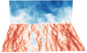
The goal of the computational model is to simulate the small-scale turbulent dynamics in the near-wall region as a function of an imposed gradient only in a small, rectangular domain $\varOmega = [0,L_x]\times [0,L_y]\times [0,L_z]$ localized to the boundary. In addition to the physical wall at $y=0$ where the no-slip condition is applied, the other computational boundaries are non-physical and located where, in a large-scale simulation, there is a region of chaotic nonlinear dynamics. At the sidewalls, periodic boundary conditions are used. This is consistent with the main scaling assumption (2.6) underlying the multiscale analysis in § 2.3, since the velocity fields evolved in time are assumed to be statistically homogeneous in the stream and spanwise directions. Any statistical inhomogeneities are modelled by $O( \epsilon )$ slow-growth terms. At the upper computational boundary $y=L_y$, homogeneous Neumann and Dirichlet conditions are prescribed for the stream/spanwise and wall-normal velocities, respectively. Since these conditions do not allow for any momentum flux through the computational boundary, the model includes a ‘fringe region’ $y \in [L_y/2, L_y]$ in which the flow is forced to provide the momentum that is transported into the near-wall region (see figure 4 for an illustration). The forcing $f$ is non-zero only in the fringe region and, given a constant pressure gradient ${\rm d}P/{{\rm d} x}$, it injects momentum in such a way that ensures that the model's wall shear stress at statistical equilibrium is unity, as in Carney et al. (Reference Carney, Engquist and Moser2020). Because of the $O( \epsilon )$ slow-growth contributions to the momentum equation derived in § 2.3, $f$ is time-dependent; the precise details are given after introducing the model equations of motion below.

Figure 4. The fluid is subject to periodic boundary conditions at the dash–dotted side walls, homogeneous Dirichlet/Neumann conditions at the upper boundary $y=L_y$ and the no-slip condition at the wall $y=0$. In addition to the constant pressure gradient assumed to be present in the near-wall layer, the model includes a time-dependent, auxiliary forcing function $f$ (depicted here at multiple realizations in time) in a ‘fringe region’ $L_y/2 \le y \le L_y$ to make up for the momentum not transported at the computational boundary $y=L_y$.

The model equations of motion posed on the domain $\varOmega$ are based on the slow-growth continuity (2.17) and momentum equations, and (2.21) from the asymptotic analysis of § 2.3, and they are discretized in the statistically homogeneous stream and spanwise directions with a Fourier–Galerkin method; however, there are a few differences in the equations that govern the horizontal averages

(3.1)\begin{equation} \bar{u}_i(y,t) = \frac{1}{L_x}\frac{1}{L_z} \int_0^{L_z} \int_0^{L_x} u_i(x,y,z,t) \, {{\rm d} x} \, {\rm d}z \end{equation}

and the fluctuations $u_i' = u_i - \bar {u}_i$.

First, the $(k_x,k_z)=(0,0)$ Fourier mode of the streamwise velocity ($\bar {u}$) evolves according to

(3.2)\begin{equation} \frac{\partial \bar{u}}{\partial t} + \frac{\partial }{\partial y}\overline{uv} + \epsilon_L \left(\overline{uu} + \frac{\partial }{\partial y} (y \overline{uu})\right) - \nu \frac{\partial^2 \bar{u}}{\partial y^2} = f-\frac{{\rm d}P}{{\rm d} x}, \end{equation}

which is simply the horizontal average of (2.21) (for $i=1$) with additional forcing terms. Here, $f$ is the fringe-region forcing whose explicit form is detailed below, while ${\rm d}P/{{\rm d} x}$ is the constant pressure gradient driving the flow in the near-wall region. Equation (3.2) is augmented with the no-slip condition at $y=0$ and the homogeneous Neumann condition $\partial _y \bar {u}=0$ at $y=L_y$. Note the parameter $\epsilon _L$ here necessarily has units of $1/{length}$, which is emphasized with the subscript ‘$L$’. After detailing the forcing $f$, $\epsilon _L$ will be related back to the non-dimensional parameter (2.3).

Taking the horizontal average of the slow-growth continuity equation (2.17) gives

(3.3)\begin{equation} \frac{\partial \bar{v}}{\partial y} + \epsilon_L \frac{\partial }{\partial y} (y \bar{u}) = 0, \end{equation}

and the no-slip condition implies that $\bar {v} = -\epsilon _L y \bar {u}$, which is of course the analogue of the relation (2.22).

In contrast to $\bar {u}$, the evolution equation for the mean spanwise velocity $\bar {w}$ is not given by the horizontal average of (2.21) for $i=3$. Instead, the $O( \epsilon )$ contributions involving $\bar {w}$ are neglected, as in Spalart (Reference Spalart1988). Using

(3.4)\begin{equation} \overline{u'w'} = \overline{uw} - \bar{u} \bar{w}, \end{equation}

$\bar {w}$ evolves as

(3.5)\begin{equation} \frac{\partial \bar{w}}{\partial t} + \frac{\partial }{\partial y}\overline{vw} + \epsilon_L \left(\overline{u'w'} + \frac{\partial }{\partial y} (y \overline{u'w'})\right) - \nu \frac{\partial^2 \bar{w}}{\partial y^2} = 0, \end{equation}

with the no-slip condition and a homogeneous Neumann condition at $y=0$ and $y=L_y$, respectively. This can be justified by the fact that the mean spanwise velocity $W = 0$ in each of the large-scale simulations listed in table 1; it does not grow. Moreover, numerical stability issues can arise if one includes the $O( \epsilon )$ contributions involving $\bar {w}$, since the laminar equation for $\bar {w}$,

(3.6)\begin{equation} \frac{\partial \bar{w}}{\partial t} - \nu \frac{\partial^2 \bar{w}}{\partial y^2} =-\epsilon_L \bar{u} \bar{w}, \end{equation}

can exhibit exponential growth. Indeed, if $\epsilon _L < 0$ (as is the case for each large-scale simulation in table 1) and $\bar {u}$ is frozen in time, then $\bar {w}\sim \exp (-\epsilon _L \bar {u} t)$.

The Fourier modes $(k_x,k_z) \ne (0,0)$ evolve as

(3.7)$$\begin{gather} \frac{\partial u_i}{\partial t} + \frac{\partial }{\partial x_j}(u_i u_j) + \epsilon_L \left(u u_i + \frac{\partial }{\partial y} (y u u_i) \right)+ \frac{\partial p}{\partial x_i} - \nu \frac{\partial^2 u_i}{\partial x_j \partial x_j} = 0, \end{gather}$$

(3.8)$$\begin{gather}\frac{\partial u_i}{\partial x_i} = 0, \end{gather}$$

in which the $O( \epsilon )$ contribution to continuity is neglected, as in Spalart (Reference Spalart1988). This appears to be a sensible approximation for boundary layers with mild $\beta$ values; recall from figure 2 that the streamwise evolution of the turbulent kinetic energy made a negligible contribution to the mean stress balances of the KS-$\beta 1$ and BVOS-$\beta 1.7$ flows in the near-wall region. The slow-growth momentum equation (3.7) is augmented with the no-slip condition $u_i=0$ at $y=0$ and the no-flux conditions

(3.9)\begin{equation} v = 0, \quad \frac{\partial u}{\partial y} = \frac{\partial w}{\partial y} = 0 \text{ at } y = L_y. \end{equation}

The model equations are solved numerically using the velocity-vorticity formulation of Kim, Moin & Moser (Reference Kim, Moin and Moser1987), which is derived from (3.7) and (3.8) in the usual way (Lee Reference Lee2015).

With all the equations of motion determined, the details of the forcing function $f$ in the mean streamwise evolution equation (3.2) can now be specified. Its role is to provide momentum that will be transported to the near-wall region, and it is non-zero only in the fringe region $y > L_y/2$. It is constructed in such a way that, for a given set of values ${\rm d}P/{{\rm d} x}$ and $\epsilon _L$, the model's equilibrium wall shear stress equals unity.

More specifically, from (3.2), the model's mean streamwise stress balance is

(3.10)\begin{equation} \tau_w + \frac{{\rm d}P}{{\rm d} x} y = \tau_{model}(y) + \int_0^y f\, {\rm d}s, \end{equation}

where, from the relation $V = -\epsilon _L y U$ (which follows from (3.3)), the model stress $\tau _{model}$ is

(3.11)\begin{equation} \tau_{model}(y) = \nu \frac{\partial U}{\partial y} - \langle u'v' \rangle - \epsilon_L \left( \int_0^y [ U^2 + \langle u'u' \rangle ] \, {\rm d}s + y \langle u'u' \rangle \right). \end{equation}

The no-flux boundary conditions imply that at $y=L_y$, (3.10) becomes

(3.12)\begin{equation} \int_{0}^{L_y} f\, {{\rm d} y} = \tau_w + \frac{{\rm d}P}{{\rm d} x} L_y + \epsilon_L \left( \int_0^{L_y} [ U^2 + \langle u'u' \rangle ] \, {{\rm d} y} + L_y \langle u'u' \rangle|_{y=L_y} \right). \end{equation}

If one then constrains $f$ to satisfy

(3.13)\begin{equation} \int_{0}^{L_y} f\, {{\rm d} y} = 1 + \frac{{\rm d}P}{{\rm d} x} L_y + \epsilon_L \left( \int_0^{L_y} [ U^2 + \langle u'u' \rangle ] \, {\rm d}s + L_y \langle u'u' \rangle|_{y=L_y} \right), \end{equation}

the desired result $\tau _w =1$ will follow. Assuming ergodicity, the identity

(3.14)\begin{equation} \langle A \rangle = \langle \bar{A} \rangle \end{equation}

is true for any field $A$. Hence, if at each point in time

(3.15)\begin{equation} \int_{0}^{L_y} f(y,t)\, {{\rm d} y} = 1 + \frac{{\rm d}P}{{\rm d} x} L_y + \epsilon_L \left( \int_0^{L_y} \overline{uu}(y,t)\, {{\rm d} y} + L_y\, \overline{u'u'}(L_y,t) \right) \end{equation}

holds, then (3.13) will result at equilibrium. The functional form of $f$ is described in § 3.3. If one additionally sets the kinematic viscosity $\nu = 1$, then at equilibrium the model is scaled in viscous units, and the parameter $\epsilon _L$ reduces to the non-dimensional $\epsilon$ introduced in (2.3).

3.2. Physical parameters

Each slow-growth near-wall patch model case is parameterized by two inputs; they are the constant mean pressure gradient scaled in wall units ${\rm d}P^+/{{\rm d} x}^+$ and the asymptotic growth parameter $\epsilon$ given by (2.3). The values for the various model cases presented – two adverse-pressure-gradient cases and one zero-pressure-gradient case – are shown in table 2. Note that for each pressure gradient value, there is a model case both with ($\epsilon \ne 0$) and without ($\epsilon =0$) growth effects included. Figure 5 illustrates the statistically converged stress balances for the three slow-growth model cases. As the imposed pressure gradient ${\rm d}P^+/{{\rm d} x}^+$ increases, the total momentum transport in the near-wall region increases, as noted in § 2.2.

Table 2. Imposed pressure gradient and slow-growth parameters for the model cases presented. Each value was chosen to match the corresponding one from the large-scale simulations listed in table 1.

Figure 5. For each case in table 1, the model stress $\tau ^+_{model}(y^+)$ (equation (3.11)) agrees with the target stress profile $\tau _{target}^+(y^+) = 1+y^+ {\rm d}P^+/{{\rm d} x}^+$ for $y^+\in [0,300]$, while in the fringe region $y^+\in [300,600]$, the primitive $F^+(y^+)$ of the forcing function $f$ supplies momentum flux so that $\tau _{model}^+(y^+)+F^+(y^+)$ agrees with the target stress throughout the entire domain $y^+\in [0,600]$. (a) SG-NWP-ZPG, (b) SG-NWP-$\beta 1$ and (c) SG-NWP-$\beta 1.7$.

3.3. Computational parameters and numerical implementation

The remaining model parameters, consistent for all simulation cases, are summarized in table 3 and are identical to those used by Carney et al. (Reference Carney, Engquist and Moser2020). In particular, the size of the rectangular domain $\varOmega$ is taken to be $L_x^+ = L_z^+ = 1500$ and $L_y^+ = 600$, selected based on the spectral analysis of Lee & Moser (Reference Lee and Moser2019). Their work suggests that, at least for the mild favourable-pressure-gradient cases considered, the contributions to the turbulent kinetic energy from modes with wavelengths $\lambda ^+ <1000$ are universal and $Re_{\tau }$ independent in the region $y^+ \lesssim 300$. Accordingly, $L_y^+$ is taken to be $2 \times 300 =600$ to allow for a sufficiently large fringe region to mollify the effect of the non-physical computational boundary at $y=L_y$ (see figure 4). The values $L_x^+ = L_z^+=1500$ were chosen because they were found to be the smallest domain sizes capable of reproducing the universal small-scale turbulent kinetic energies identified in the channel flow simulations of Lee & Moser (Reference Lee and Moser2019) (see § 3.3 of Carney et al. Reference Carney, Engquist and Moser2020). The majority of statistics reported in this work were from simulations with these stream and spanwise dimensions; however, a range of values larger than 1500 were also explored to assess the dependence of the model statistics on the choice of $L_x$ and $L_z$. In general, the statistics generated from these simulations exhibit little to no variation as the domain sizes grow. The streamwise and spanwise velocity variances are two exceptions to this, however. As discussed more fully in § 4.2, these statistics are known to be influenced by low-wavenumber, large-scale structures present in direct numerical simulations. As the NWP domain sizes grow, more of these large-scale structures are included, and hence the stream/spanwise velocity variances continually change with increasing $L_x$ and $L_z$. The results are documented in the Appendix.

Table 3. Summary of simulation parameters consistent for all simulation cases; $N_x$ and $N_z$ refer to the number of Fourier modes, while $N_y$ is the number of B-spline collocation points. Here, $\Delta x = L_x/N_x$ and similarly for $\Delta z$, and $\Delta y_w$ is the collocation point spacing at the wall.

For a given selection of model parameters $({\rm d}P^+/{{\rm d} x}^+, \epsilon )$, the forcing function $f$ responsible for providing momentum flux to the near-wall region is constrained at each time step to satisfy (3.15); otherwise, however, it is not uniquely specified. For the simulations reported here, $f$ is taken to be $f(y,t) = \psi (t) g(y)$, where $g$ is a piecewise cubic function

(3.16)\begin{equation} g(y) = \left\{\begin{array}{@{}ll} 4/L_y^4 (L_y-2y)^2 (5L_y-4y) & y \in [L_y/2,L_y] \\ 0 & y \in [0,L_y/2] \end{array}\right., \end{equation}

which satisfies

(3.17)\begin{equation} \int_{L_y/2}^{L_y}g(y)\, {{\rm d} y} = 1, \end{equation}

and $g(L_y/2)= g'(L_y/2) = g'(L_y) = 0$, so that the transition in forcing from the near-wall region to the fringe region is smooth. In general, other function forms for $g$ are of course possible and, in particular, a quadratic profile satisfying (3.17) and $g(L_y/2)=g'(L_y/2)=0$ was also implemented with no discernible changes in the statistics in the near-wall region $y^+\in [0,300]$. The time-dependent function $\psi$ is defined as

(3.18)\begin{equation} \psi(t) = 1 + \frac{{\rm d}P}{{\rm d} x}L_y + \epsilon_L \left( \int_0^{L_y} \overline{uu}(y,t) \, {{\rm d} y} + L_y \overline{u'u'} (L_y,t)\right), \end{equation}

which is simply the right-hand side of the forcing constraint (3.15). Together, (3.17) and (3.18) ensure that the constraint (3.15) indeed holds.

As mentioned in § 3.1, the model is solved numerically using the velocity-vorticity formulation of Kim et al. (Reference Kim, Moin and Moser1987). The numerical method is identical to that employed by Carney et al. (Reference Carney, Engquist and Moser2020) and Lee & Moser (Reference Lee and Moser2015), that is, a Fourier–Galerkin method and a seventh-order B-spline collocation method for the stream/spanwise directions and wall-normal direction, respectively. The equations of motion are integrated in time with a low-storage, third-order Runge–Kutta (RK) method that treats diffusive terms implicitly and convective terms explicitly (Spalart, Moser & Rogers Reference Spalart, Moser and Rogers1991). Note that the forcing term $f(y,t)$ in the evolution equation (3.2) for $\bar {u}$ is a nonlinear (and non-local) expression, and it is thus treated explicitly in the RK scheme, like the other nonlinear terms.

The computational resolution in both time and space is chosen to be consistent with that of channel flow DNS. The number of Fourier modes (and corresponding effective resolutions) used in each model simulation are listed in table 3. They are comparable with, for example, the parameters listed in table 1 of Lee & Moser (Reference Lee and Moser2015). Additionally, the collocation point spacing in the wall-normal direction is similar to previous DNS studies; the total number of collocation points $N_y$ below $y^+ = 600$, as well as their distribution $\Delta y^+$ in the near-wall region, are taken to be equal to the $Re_{\tau } = 1000$ case of Lee & Moser (Reference Lee and Moser2015). As done by Carney et al. (Reference Carney, Engquist and Moser2020), the model is implemented in a modified version of the PoongBack DNS code (Lee, Malaya & Moser Reference Lee, Malaya and Moser2013; Lee et al. Reference Lee, Ulerich, Malaya and Moser2014).

3.4. Statistical convergence

The method of Oliver et al. (Reference Oliver, Malaya, Ulerich and Moser2014) is used to assess the uncertainty in the statistics reported due to sampling error. For each $({\rm d}P^+/{{\rm d} x}^+, \epsilon )$ case listed in table 2, the statistics are collected by averaging in time until the estimated statistical uncertainty in the total model stress profile $\tau _{model}(y)$ (see (3.11)) is less than a few per cent. Figure 6 shows that the sampling error $|\tau ^+_{model}(y^+)-\tau _{target}^+(y^+)|$ (where $\tau _{target}(y) = \tau _w + y\, {\rm d}P/{{\rm d} x}$) is no larger than three per cent for each SG model case and, in particular, the errors are smaller than the uncertainties; the errors are similarly small for the $\epsilon =0$ cases (not displayed).

Figure 6. Statistical convergence for the slow-growth model cases listed in table 2: solid lines, absolute error $|\tau _{model}^+(y^+) - \tau _{target}^+(y^+)|$, where $\tau _{model}$ is defined in (3.11) and $\tau _{target} = \tau _w + y\, {\rm d}P/{{\rm d} x}$; dash–dotted lines, standard deviation of the estimated statistical error for $\tau _{model}^+$ in the region $y^+ \in [0,300]$. (a) SG-NWP-ZPG, (b) SG-NWP-$\beta 1$ and (c) SG-NWP-$\beta 1.7$.

4.1. Mean velocity and shear stresses

Because the Reynolds stress of a zero-pressure-gradient boundary layer is dominated by small-scale near-wall turbulent fluctuations and growth effects are relatively insignificant, the mean velocity and Reynolds shear stress profiles from the NWP-ZPG model case are in excellent agreement with the corresponding DNS profiles (Carney et al. Reference Carney, Engquist and Moser2020). The $O( \epsilon )$ terms included in the SG-NWP-ZPG case only enhance the agreement; in particular, there is a modest improvement in the Reynolds stress profile for $y^+ \in [100,300]$ from the NWP-ZPG case that reduces the maximum relative error from 4 % to 1.3 %, as shown in figure 7(c). The slow-growth terms seem to not have an effect on the mean velocity $U^+$, as the NWP-ZPG and SG-NWP-ZPG profiles are nearly identical. In both cases, the relative error in $U^+$ is less than $0.6\,\%$ for $y^+ \in [0,300]$, and the error is similarly small for the log-law indicator function $\gamma ^+$,

(4.1)\begin{equation} \gamma^+(y^+) = y^+ \frac{\partial U^+}{\partial y^+} , \end{equation}

in the range $y^+\in [0,100]$. However, in both cases, there is mild disagreement of $\gamma$ in the range $y^+ \in [100,300]$. As expected, the profiles diverge for $y^+>300$; recall that $\langle u'v' \rangle$ necessarily vanishes as a consequence of the $v=0$ condition posed (for Fourier modes $(k_x,k_z) \ne (0,0)$) at the upper computational boundary $y=L_y$.

Figure 7. (a) Mean velocity $U^+$, (b) indicator function $\gamma ^+=y^+ \partial U^+/\partial y^+$ and (c) Reynolds stress $\langle u'v' \rangle ^+$ versus $y^+$ for the zero-pressure-gradient simulation cases. The vertical, black dash–dotted lines mark the beginning of the fringe region $y^+=300$, and the law-of-the-wall $U^+ = y^+$ and $U^+ = (1/\kappa ) \log (y^+) + B$ is also marked with a red dash–dotted line in panel (a), where $\kappa = 0.384$ and $B = 4.27$ (Lee & Moser Reference Lee and Moser2015).

Since growth effects fundamentally alter the balance of momentum transport in the near-wall region for adverse-pressure-gradient boundary layers (recall figure 2), the model cases NWP-$\beta 1$ and NWP-$\beta 1.7$ that do not account for these effects are not expected to accurately reproduce the Reynolds shear stress profiles from the corresponding DNS and wall-resolved (WR)LES cases KS-$\beta 1$ and BVOS-$\beta 1.7$. Figure 8 indeed shows that this is the case; when $\epsilon =0$, the model severely overestimates the target profiles for $y^+ \in [70,300]$. Including the $O( \epsilon )$ terms from the slow-growth analysis, however, leads to a significant improvement, as the SG-NWP-$\beta 1$ and SG-NWP-$\beta 1.7$ model cases both have a maximum error of approximately 9 % and 7 %, respectively, for $y^+\in [0,300]$. This remarkable improvement demonstrates that the SG-NWP model's $O( \epsilon )$ terms, as well as the forcing function $f$ in the fringe-region $300 \le y^+\le 600$, provide a good approximation of the momentum transport environment present in real, spatially developing wall-bounded turbulent flows with mild adverse pressure gradients.

Figure 8. (a) Mean velocity $U^+$, (b) indicator function $\gamma ^+=y^+ \partial U^+/\partial y^+$ and (c) Reynolds stress $\langle u'v' \rangle ^+$ versus $y^+$ for the adverse-pressure-gradient simulation cases. The vertical, black dash–dotted lines mark the beginning of the fringe region $y^+=300$, and the law-of-the-wall $U^+ = y^+$ and $U^+ = (1/\kappa ) \log (y^+) + B$ is also marked with a red dash–dotted line in panel (a), where $\kappa = 0.384$ and $B = 4.27$ (Lee & Moser Reference Lee and Moser2015).

Similar to the zero-pressure-gradient case, the mean velocity and log-law indicator profiles for the adverse-pressure-gradient model flows are essentially identical whether or not slow-growth effects are included. For all four adverse-pressure-gradient model cases, the relative error in the mean velocity profile $U^+$ is less than 6 % in the near-wall region $y^+ \in [0,300]$. The error in the log-law indicator function $\gamma ^+$ is similarly small for $y^+ \in [0,80]$, while each model case underpredicts $\gamma$ for $y^+ \in [80, 300]$. However, this underprediction appears to be slightly worse for the SG-NWP cases than for those with $\epsilon =0$. From the mean stress balance (3.10), for $\epsilon =0$, overprediction of the Reynolds shear stress implies underprediction of the mean viscous stress, however, the slow-growth terms present in (3.10) appear to be responsible for the underprediction when $\epsilon \ne 0$, given that the Reynolds stress is more accurate. As discussed in § 2.1, it is expected that the accuracy of the model would increase in the region $y^+\in [80,300]$ if it were compared with a DNS/WRLES flow at the same pressure gradient ${\rm d}P^+/{{\rm d} x}^+$ and growth parameter $\epsilon$ but larger $Re_{\tau }$.

4.2. Velocity variances

For a wall-bounded flow in a full size domain, the low-wavenumber contributions to the Reynolds stress represent the mean influences of the large-scale structures on the near-wall dynamics. It is well established that for channel and zero-pressure-gradient boundary layer flows, these low-wavenumber features of the near-wall flow depend on $Re_{\tau }$ (Hutchins & Marusic Reference Hutchins and Marusic2007; Marusic et al. Reference Marusic, Mathis and Hutchins2010a; Lee & Moser Reference Lee and Moser2017; Samie et al. Reference Samie, Marusic, Hutchins, Fu, Fan, Hultmark and Smits2018; Lee & Moser Reference Lee and Moser2019). Their contribution to the turbulent kinetic energy and their modulation of the small-scale, high-wavenumber energy both increase with increasing $Re_{\tau }$. Experimental (Harun et al. Reference Harun, Monty, Mathis and Marusic2013; Sanmiguel Vila et al. Reference Sanmiguel Vila, Örlü, Vinuesa, Schlatter, Ianiro and Discetti2017, Reference Sanmiguel Vila, Vinuesa, Discetti, Ianiro, Schlatter and Örlü2020) and computational (Lee Reference Lee2017; Yoon et al. Reference Yoon, Hwang and Sung2018; Tanarro et al. Reference Tanarro, Vinuesa and Schlatter2020; Pozuelo et al. Reference Pozuelo, Li, Schlatter and Vinuesa2022) studies have demonstrated that a similar result holds for adverse-pressure-gradient boundary layers; increasing the pressure gradient parameter $\beta$ leads to a significant enhancement of the large-scale energy, both in the outer layer and in the near-wall region.

The SG-NWP model, by design, cannot accurately represent these large-scale structures, as it instead seeks to isolate the dynamics of the near-wall small-scales associated with the autonomous cycle of Jiménez & Pinelli (Reference Jiménez and Pinelli1999) from their influence. Since the stream and spanwise velocity variances in both the zero and adverse-pressure-gradient boundary layers considered here are known to depend on low-wavenumber contributions, the corresponding model profiles are not expected to be accurate. Figure 9 shows this is indeed the case. Although both the NWP-ZPG and SG-NWP-ZPG $\langle u'u' \rangle$ profiles appear to be in excellent agreement with the corresponding profile from Sillero et al. (Reference Sillero, Jiménez and Moser2013), this is a serendipitous coincidence. For an experiment or simulation at a larger $Re_{\tau }$, the streamwise velocity variance will grow (see figure 2 of Samie et al. (Reference Samie, Marusic, Hutchins, Fu, Fan, Hultmark and Smits2018), for example), but it will be modelled by a similar SG-NWP flow; although $\epsilon$ may differ slightly, the pressure gradient will be the same. Similarly, at first glance, the model $\langle u'u' \rangle$ profiles in the adverse-pressure-gradient cases (figure 9d–f) are seen to be significantly larger than their large-scale simulation counterparts. However, it should be noted that the KS-$\beta 1$ and BVOS-$\beta 1.7$ simulations are at relatively low $Re_{\tau }$ (see table 1); at fixed $\beta$ values but larger $Re_{\tau }$, the profiles would be larger (Sanmiguel Vila et al. Reference Sanmiguel Vila, Vinuesa, Discetti, Ianiro, Schlatter and Örlü2020; Pozuelo et al. Reference Pozuelo, Li, Schlatter and Vinuesa2022).

Figure 9. Velocity variances $\langle u'_{\alpha } u'_{\alpha } \rangle$ versus $y^+$ for (a–c) zero-pressure-gradient and (d–f) adverse-pressure-gradient simulations. The vertical, black dash–dotted lines mark the beginning of the fringe region $y^+=300$.

In contrast to the stream and spanwise velocity variances, the impact of large-scale motions on the wall-normal velocity variance for zero and adverse-pressure-gradient boundary layers is less well documented. For channel flows, Lee & Moser (Reference Lee and Moser2019) established that the $\langle v'v' \rangle$ energy density in the near-wall region is concentrated primarily at wavelengths less than $1000$ in viscous units, and hence the near-wall patch profiles from Carney et al. (Reference Carney, Engquist and Moser2020) were indeed in agreement with those from large-scale simulations. Figure 9 suggests a similar result holds true for the near-wall region of adverse-pressure-gradient boundary layers. Although the agreement is not as good as the zero-pressure-gradient cases, the SG-NWP model $\langle v'v' \rangle$ profiles compare reasonably well with the KS-$\beta 1$ and BVOS-$\beta 1.7$ data; the maximum relative error for $y^+ \in [0,300]$ is 14 % and 8.5 %, respectively. The NWP model without slow-growth effects, however, overpredicts the adverse-pressure-gradient wall-normal velocity variance, similar to the Reynolds shear stress profiles, illustrating the impact of the streamwise development of the mean wall shear stress $\tau _w$ on the near-wall turbulent kinetic energy.

4.3. Small-scale turbulent kinetic energy

Universal small-scale dynamics in the near-wall region associated with the autonomous cycle of Jiménez & Pinelli (Reference Jiménez and Pinelli1999) have been identified in channels (Lee & Moser Reference Lee and Moser2019) and zero-pressure-gradient boundary layers (Samie et al. Reference Samie, Marusic, Hutchins, Fu, Fan, Hultmark and Smits2018) by applying a high-pass filter to the energy spectral density. Increases in the near-wall, small-scale energy have also been reported in adverse-pressure-gradient boundary layers due to amplitude modulation effects (Harun et al. Reference Harun, Monty, Mathis and Marusic2013; Lee Reference Lee2017; Yoon et al. Reference Yoon, Hwang and Sung2018). Sanmiguel Vila et al. (Reference Sanmiguel Vila, Vinuesa, Discetti, Ianiro, Schlatter and Örlü2020) explicitly computed small-scale contributions to the near-wall turbulent kinetic energy. Using a cutoff wavelength of $\lambda _x^+ \approx 4300$, they found a collapse in the peak of the small-scale contribution to $\langle u'u' \rangle ^+$ at $y^+ \approx 15$ for a range of $\beta$ values from $0$ to approximately $2.2$. In contrast, Lee (Reference Lee2017) found that the small-scale contributions to the streamwise velocity variance increased with the pressure gradient, however, this result was based on a much more restrictive high-pass filter; all contributions from spanwise wavelengths $\lambda _z^+ \gtrsim 180$ were filtered out. Using the same filter as Carney et al. (Reference Carney, Engquist and Moser2020) defined by (4.2) below, the small-scale near-wall energy from SG-NWP flows is found to increase with increasing pressure gradient, in agreement with the conclusion of Lee (Reference Lee2017).

Carney et al. (Reference Carney, Engquist and Moser2020) directly compared the near-wall patch model's high-pass filtered Reynolds stress to the filtered profiles of several channel flow DNS of Lee & Moser (Reference Lee and Moser2019). After filtering out contributions from wavemodes that do not satisfy

(4.2)\begin{equation} \min\{ |k_x|, |k_z| \} > k_{cut} , \end{equation}

where $k_{cut} = 2{\rm \pi} /\lambda _{cut}$ and $\lambda _{cut}^+=1000$, the model's Reynolds stress profiles were in close agreement with the filtered DNS profiles, indicating the NWP model successfully reproduces the universal small-scale dynamics. Although the high-pass filtered Reynolds stresses of the present slow-growth NWP model cannot be directly compared with data from the literature, we report them here nonetheless to illustrate the effect of pressure gradient and growth on the small-scale energies.

Let $\mathcal {K}$ denote the set of all wavenumbers included in an SG-NWP simulation, and let $k_{\rm } = 2{\rm \pi} /\lambda _{cut}$ with $\lambda ^+_{cut} = 1000$ as just mentioned. Define $\mathcal {K}_{SS}$ to be the subset of $\mathcal {K}$ with the property that $(k_x,k_z) \in \mathcal {K}_{SS}$ if (4.2) holds. If $E_{ij}$ denotes the Fourier transform of the two point correlation tensor

(4.3)\begin{equation} R_{ij} (r_x,y,r_z) = \langle u_i'(x + r_x, y, z + r_z) u_j'(x,y,z) \rangle \end{equation}

in the variables $r_x$ and $r_z$, then the small-scale energies shown in figure 10 are defined to be

(4.4)\begin{equation} \langle u_i'u_j' \rangle_{SS} (y) = \sum_{(k_x,k_z) \in \mathcal{K}_{SS} } E_{ij} (k_x, y, k_z) . \end{equation}

It is clear that for each component $\langle u'_{\alpha }u'_{\alpha } \rangle$, the model's near-wall, small-scale energy increases as the pressure gradient ${\rm d}P^+/{{\rm d} x}^+$ increases, whether or not slow-growth effects are included. The agreement between simulations with and without $O( \epsilon )$ terms is particularly strong for the streamwise small-scale energy in the region $y^+ \lesssim 50$, suggesting that the increase in small-scale, near-wall energy in this region can be attributed solely to the adverse-pressure-gradient effects, and not to growth effects.

Figure 10. High-pass filtered velocity variances $\langle u'_{\alpha } u'_{\alpha } \rangle _{SS}$ versus $y^+$ for each model case listed in table 2. The vertical, black dash–dotted lines mark the beginning of the fringe region $y^+=300$.

4.4. Turbulent kinetic energy budget

The mean dynamics of the turbulent kinetic energy $k = u_i'u_i'/2$ are governed by the turbulent kinetic energy (TKE) budget equation

(4.5)\begin{equation} \frac{{\rm D} \langle k \rangle}{{\rm D}t} =- \overbrace{\langle u_i'u_j' \rangle\frac{\partial U_i}{\partial x_j}}^{\mathcal{P}_{k}} - \overbrace{\frac{\partial \langle ku_j' \rangle}{\partial x_j}}^{T_{k}} + \overbrace{\nu \frac{\partial^2 \langle k \rangle}{\partial x_j\partial x_j}}^{D_{k}} - \overbrace{\frac{\partial \langle \,p'u_j' \rangle}{\partial x_j}}^{\varUpsilon_{k}} - \overbrace{\nu \left\langle \frac{\partial u_i'}{\partial x_j}\frac{\partial u_i'}{\partial x_j} \right\rangle}^ {\varepsilon_{k}}. \end{equation}

For a wall-bounded turbulent flow that is homogeneous in the spanwise direction and slowly developing in the streamwise direction, one can derive a ‘slow-growth’ version of (4.5) using the same multiscale asymptotic analysis outlined in § 2.3; namely, one transforms $x$ and $y$ according to (2.8) and then inserts the scaling ansatz (2.6) into the resulting equation. The resulting ‘slow-growth’ TKE budget equation can be shown to be

(4.6)\begin{align} \overbrace{2\epsilon \langle k \rangle^+ U^+ }^{\textrm{SG Adv.}} &=- \overbrace{\left( \langle u'v' \rangle^+ \frac{\partial U^+}{\partial y^+} + \epsilon \frac{\partial }{\partial y^+}(y^+U^+) [\langle u'u' \rangle^+- \langle v'v' \rangle^+] \right)}^{\mathcal{P}^+_{k,SG}} \nonumber\\ &\quad - \overbrace{\left( \frac{\partial }{\partial y^+}\langle kv' \rangle^++ 3 \epsilon \langle ku' \rangle^++ \epsilon\, y^+ \frac{\partial }{\partial y^+} \langle ku' \rangle^+ \right)}^{T^+_{k,SG }} \nonumber\\ &\quad - \overbrace{\left(\frac{\partial }{\partial y^+} \langle \,p'v' \rangle^++ 3\epsilon \langle \,p'u' \rangle^++ \epsilon \, y^+ \frac{\partial }{\partial y^+} \langle \,p'u' \rangle^+ \right)}^{\varUpsilon^+_{k, SG}} \nonumber\\ &\quad + \overbrace{\frac{\partial^2 }{(\partial y^+)^2}\langle k \rangle^+}^{D^+_{k,SG}} - \overbrace{\left\langle \frac{\partial u_i'}{\partial x_j}\frac{\partial u_i'}{\partial x_j} \right\rangle^+}^{\varepsilon^+_{k,SG}}, \end{align}

where the $O( \epsilon ^2 )$ contributions are neglected. If one alternatively starts with the slow-growth continuity (2.17) and momentum (2.19) equations from § 2.3 and derives an equation governing the dynamics of $\langle u_i'u_i' \rangle ^+/2$ in the standard way, then, modulo $O( \epsilon ^2 )$ terms, nearly the same exact equation will result. The only difference is that, in this latter derivation, an extra $O( \epsilon )$ correction to the dissipation $\varepsilon _k$ appears that is not present in (4.6). The term is proportional to $y\langle u_i' \partial _x \partial _y u_i' \rangle$ and arises from the $O( \epsilon )$ viscous term in (2.19).

Because the SG-NWP model momentum equation (3.7) neglects some of the $O( \epsilon )$ terms that arise from the asymptotic analysis in § 2.3, there are some discrepancies between (4.6) and the model's TKE budget equation. In particular, there are discrepancies in the production $\mathcal {P}_{k,SG}$, as well as the turbulent and pressure transport terms $T_{k,SG}$ and $\varUpsilon _{k,SG}$. Although the errors introduced by these discrepancies are in each case relatively small, they are documented below when comparing the model's TKE budget to those of the large-scale simulations.

First, since the mean advection $U^+ \partial _x^+ \langle k \rangle ^+ + V^+\partial _y^+ \langle k \rangle ^+$ from the large-scale simulations and the slow-growth advection

(4.7)\begin{equation} 2\epsilon \langle k \rangle^+ U^+ \end{equation}

from the NWP model cases have a maximum value no larger than $10^{-3}$, they are not plotted here.

For the production $\mathcal {P}_{k, SG}$, the inconsistency between the continuity equations (2.17) and (3.8) leads to some ‘spurious’ $O( \epsilon )$ production terms for the SG-NWP model given by

(4.8)\begin{equation} \mathcal{P}^+_{k,spur} = \epsilon \left( U^+ \langle u'u' \rangle^++ \frac12 y^+ U^+ \frac{\partial }{\partial y^+}\langle u'u' \rangle^+\right). \end{equation}

Figure 11(a,c) displays $\mathcal {P}^+_k$ from (4.5) for the large-scale simulation cases, and the sum of $\mathcal {P}_{k, SG}^+$ from (4.6) and the spurious production (4.8) for the SG-NWP flows. Note that for the zero and adverse-pressure-gradient flows considered in this work, production is due almost exclusively to the product of $\partial U/\partial y$ and the Reynolds shear stress. For example, this term accounts for approximately $97.5$ % of the total production for the three large-scale flows from table 1. Similarly, the $O( \epsilon )$ terms account for only $0.2$ %, $5.7$ % and $4.7$ % of the SG model's production $\mathcal {P}_{k, SG}^+$ for $y^+\in [0,300]$ for SG-NWP-ZPG, SG-NWP-$\beta 1$ and SG-NWP-$\beta 1.7$, respectively, while the spurious production (4.8) is no larger than $0.1$ %, $3.7$ % and $3.4$ % of $\mathcal {P}_{k,SG}^+$ for these three model cases.

Figure 11. (a,c) Production of TKE versus $y^+$, where the results from the large-scale simulations display $\mathcal {P}_k^+$ from (4.5), while the model results display the sum of $\mathcal {P}_{k,SG}^+$ from (4.6) and (4.8); (b,d) Dissipation of TKE versus $y^+$. For both quantities, the ZPG and APG flows are displayed in panels (a,b) and (c,d), respectively. The vertical, black dash–dotted lines mark the beginning of the fringe region $y^+=300$.

As expected, there is little difference between the SG-NWP-ZPG and NWP-ZPG production profiles, since the mean velocity gradient and Reynold shear stress profiles for both model flows are nearly identical. Both are in excellent agreement with the SJM-$\beta 0$ DNS case. For the adverse-pressure-gradient cases, the SG-NWP model's production $\mathcal {P}^+_{k, SG} + \mathcal {P}^+_{k,spur}$ is consistently smaller than the corresponding cases when $\epsilon =0$. At the near-wall production peak ($y^+\approx 12$), this results in better agreement with the BVOS-$\beta 1.7$ case for the SG-NWP model than the $\epsilon =0$ case, while for the KS-$\beta 1$ case, the agreement is slightly worse. In both cases, the slow-growth model underpredicts the production profiles from the large-scale simulations for $y^+ \gtrsim 60$, consistent with the results for the mean streamwise velocity gradient.

Unlike the production of turbulent kinetic energy, the dissipation $\varepsilon _{k} = \nu \langle \partial _j u_i'\partial _j u_i' \rangle$ does not possess any additional slow-growth contributions, as previously noted. Figure 11(b,d) displays the dissipation profiles for the model and large-scale simulation cases. Although there is no discernible difference between the NWP model with and without slow-growth effects in the zero-pressure-gradient case, they do impact the model dissipation profiles in the adverse-pressure-gradient cases. In particular, they effect a reduction in the maximum dissipation that occurs at the wall, resulting in better agreement with the large-scale simulation values.

Similar to the dissipation, the viscous transport does not possess any $O( \epsilon )$ slow-growth contributions. However, there are indeed some $O( \epsilon )$ ‘spurious’ contributions to the SG-NWP model's turbulent transport given by

(4.9)\begin{equation} T^+_{k,spur} = \epsilon \left( \langle ku' \rangle^++ y^ + \left\langle k\frac{\partial u'}{\partial y} \right\rangle^+ \right) \end{equation}

that arise from omitting the $O( \epsilon )$ contribution to the fluctuating continuity equation (2.17). The omission of both this term and the $O( \epsilon )$ pressure term in (2.19) from the SG-NWP model equations also leads to some errors in the pressure transport. In particular, the model's pressure transport does not include any slow-growth contributions, in contrast to $\varUpsilon _{k,SG}$, so that in effect there is a spurious contribution given by

(4.10)\begin{equation} \varUpsilon^+_{k,spur} =-\epsilon \left( 3 \langle \,p'u' \rangle^+ + y^+ \frac{\partial }{\partial y^+} \langle \,p'u' \rangle^+\right). \end{equation}

The SG-NWP turbulent $T^+_{k, SG} + T^+_{k,spur}$, pressure $\varUpsilon ^+_{k,SG} + \varUpsilon ^+_{k,spur}$ and viscous $D^+_{k,SG}$ transport profiles are displayed in figure 12 and show a reasonable agreement to the corresponding profiles $T^+_k$, $\varUpsilon ^+_k$ and $D^+_k$ (as defined in (4.5)) from the large-scale simulations. In particular, the SG-NWP model predicts a lower value of viscous transport at the wall than the corresponding model simulations with $\epsilon =0$, similar to the dissipation profiles. In contrast, the pressure transport at the wall is notably less accurate when including slow-growth effects. The error is not due to the spurious pressure transport; the spurious terms generally contribute no more than $5$ % to the model's total turbulent and pressure transport profiles, similar to the TKE production. Since pressure is generally responsible for enforcing continuity, it is possible that the $O( \epsilon )$ error in the fluctuating SG continuity equation (3.8) is responsible for the relatively large error. It would be useful to test this hypothesis in future work; a reformulation of the velocity-vorticity method due to Kim et al. (Reference Kim, Moin and Moser1987) used here will be required to account for the fact that the velocity fluctuations are not divergence free.

Figure 12. (a,d) Turbulent, (b,e) pressure and (c,f) viscous transport of TKE versus $y^+$. The results from the large-scale simulations display $T_k^+$, $\varUpsilon _k^+$ and $D_k^+$ from (4.5), respectively, while the model results display $T^+_{k,SG}+T^+_{k,spur}$, $\varUpsilon ^+_{k,SG} + \varUpsilon ^+_{k,spur}$ and $D_k^+$. The vertical, black dash–dotted lines mark the beginning of the fringe region $y^+=300$.