


1. Introduction
With the rise of population in urban areas, understanding how pollutants remain trapped within metropolitan regions is of increasing importance. Recently reported as the largest environmental health risk in Europe (Lelieveld et al. Reference Lelieveld, Klingmüller, Pozzer, Pöschl, Fnais, Daiber and Münzel2019), air pollution is a major cause of premature deaths and disease. Therefore, predictive models for air-quality control are relevant to provide protection from excessive pollutant concentrations. The essential need to address sustainable development from an urban perspective is enshrined in the 2030 Agenda (United Nations 2015) through the sustainable development goals 11 and 13, on sustainable cities and climate action, respectively. However, the available models are unable to provide the required spatio-temporal accuracy to reproduce the pollutant-dispersion patterns within cities (Torres, Le Clainche & Vinuesa Reference Torres, Le Clainche and Vinuesa2021). Improved prediction and assessment techniques are needed urgently to address these issues and promote urban sustainability in the near future (Vinuesa et al. Reference Vinuesa, Schlatter, Malm, Mavriplis and Henningson2015). In this study, we propose an information-theoretic analysis through causality metrics of a reduced-order model (ROM) of the flow around a wall-mounted square cylinder to gain further insight into the underlying mechanisms defining the flow, shedding light on new possibilities for future urban-flow control research. Note that although the considered flow case is significantly simpler than that in an urban environment, the focus here is in the arch vortices, which are present in the analysed flow and have an important role in pollutant transport in cities (Monnier et al. Reference Monnier, Goudarzi, Vinuesa and Wark2018; Lazpita et al. Reference Lazpita, Martínez-Sánchez, Corrochano, Hoyas, Le Clainche and Vinuesa2022).
The flow around this type of environment is generally found to be turbulent. Due to the wide range of spatio-temporal features present in such a high-dimensional nonlinear chaotic system, these flows are challenging to analyse. However, the presence of similar flow characteristics across a plethora of fluid flows has revealed the presence of dominant processes that constitute the basis of various types of flow. Modal-decomposition techniques offer the possibility to analyse nonlinear and chaotic dynamics, and create ROMs by defining a low-dimensional coordinate system for capturing dominant flow characteristics. Proper orthogonal decomposition (POD) (Lumley Reference Lumley1967) and dynamic mode decomposition (DMD) (Rowley et al. Reference Rowley, Mezić, Bagheri, Schlatter and Henningson2009; Schmid Reference Schmid2010) are two modal-decomposition methods based on linear algebra that have been used widely to extract the dominant spatio-temporal features in fluid flows. Balanced POD (BPOD) (Rowley Reference Rowley2005), spectral POD (SPOD) (Towne, Schmidt & Colonius Reference Towne, Schmidt and Colonius2018), higher-order DMD (HODMD) (Le Clainche & Vega Reference Le Clainche and Vega2017) and spatio-temporal Koopman decomposition (STKD) (Le Clainche & Vega Reference Le Clainche and Vega2018) are several successful variants of POD and DMD for analysis of turbulent flows. These techniques have been assessed in the context of simplified urban flows in the recent works of Lazpita et al. (Reference Lazpita, Martínez-Sánchez, Corrochano, Hoyas, Le Clainche and Vinuesa2022) and Martínez-Sánchez et al. (Reference Martínez-Sánchez, Lazpita, Corrochano, Le Clainche, Hoyas and Vinuesa2023). They analysed the near-wake flow of finite square cylinders, which can be described as a combination of four main vortices (Hunt et al. Reference Hunt, Abell, Peterka and Woo1978; Wang & Zhou Reference Wang and Zhou2009): the tip (or roof) vortex, the spanwise vortex, the base vortex (a streamwise vortex formed near the cylinder base with close interaction with the wake) and the horseshoe vortex, which forms around the obstacle. The well-known arch vortex can be then described as a combination of the first three (Sakamoto & Arie Reference Sakamoto and Arie1983; Tanaka & Murata Reference Tanaka and Murata1999; Wang et al. Reference Wang, Zhou, Chan and Lam2006; Wang & Zhou Reference Wang and Zhou2009), resulting in a vortical structure forming on the leeward side of a wall-mounted obstacle that consists of two legs and one roof. The flow rotates in the spanwise direction in the former vortex features, and in the wall-normal direction in the latter one. This vortex has been studied extensively by the fluid mechanics community, both experimentally (Hunt et al. Reference Hunt, Abell, Peterka and Woo1978; Oke Reference Oke1988; Becker, Lienhart & Durst Reference Becker, Lienhart and Durst2002; AbuOmar & Martinuzzi Reference AbuOmar and Martinuzzi2008; Zajic et al. Reference Zajic, Fernando, Calhoun, Princevac, Brown and Pardyjak2011; Kawai, Okuda & Ohashi Reference Kawai, Okuda and Ohashi2012; Zhu et al. Reference Zhu, Wang, Wang and Wang2017; Monnier et al. Reference Monnier, Goudarzi, Vinuesa and Wark2018) and numerically (Sohankar, Norberg & Davidson Reference Sohankar, Norberg and Davidson1999; Saha, Biswas & Muralidhar Reference Saha, Biswas and Muralidhar2003; Vinuesa et al. Reference Vinuesa, Schlatter, Malm, Mavriplis and Henningson2015; Amor et al. Reference Amor, Pérez, Schlatter, Vinuesa and Le Clainche2020; Torres et al. Reference Torres, Le Clainche and Vinuesa2021), due to its implications in urban environment phenomena, i.e. pollutant dispersion, air quality, heat propagation and impact on pedestrian comfort (Oke Reference Oke1988).
The flow around these wall-mounted obstacles is also strongly three-dimensional. Martinuzzi & Tropea (Reference Martinuzzi and Tropea1993) compared to the characteristics of the flow around two-dimensional and three-dimensional obstacles of different width-to-height ratios, and highlighted their three-dimensionality as a result of flow separation. As the flow encounters the obstacle initially, a recirculation bubble formed on the windward side of the cylinder induces an adverse pressure gradient that thickens the incoming boundary layer, which then produces a shear layer around the obstacle (Becker et al. Reference Becker, Lienhart and Durst2002; Wang & Zhou Reference Wang and Zhou2009). Simultaneously, a horseshoe vortex progressively gets wider around the two sides of the cylinder, a fact that accelerates the flow close to the obstacle due to the favourable pressure gradient induced by the geometry (Hunt et al. Reference Hunt, Abell, Peterka and Woo1978). A separated wake is then formed downstream of the obstacle with a self-sustained oscillation process and a downward motion from the top of the obstacle, which is responsible for the widening of the wake (Straatman & Martinuzzi Reference Straatman and Martinuzzi2003; Vinuesa et al. Reference Vinuesa, Schlatter, Malm, Mavriplis and Henningson2015).
The topology of the near-wake flow consists of free-end downwash flow, spanwise shear flow and upwash flow from the wall, which relate to the tip, base and spanwise vortices (Wang & Zhou Reference Wang and Zhou2009). The formation of the arch vortex is produced as a result of the previous flow features, and they are closely related to the symmetric shedding modes, which induce an arch-type structure even on the instantaneous field (Zhu et al. Reference Zhu, Wang, Wang and Wang2017). Using various modal-decomposition methods, Lazpita et al. (Reference Lazpita, Martínez-Sánchez, Corrochano, Hoyas, Le Clainche and Vinuesa2022) assessed the characteristics of the arch vortex and documented the generation and destruction mechanisms of this vortex based on the resulting spatio-temporal modes, which were classified as vortex-generator and vortex-breaker modes, respectively. As a result, they suggested that the arch vortex may be connected with the dispersion of pollutants in urban environments, where its generation leads to an increase in their concentration. Other studies (Bourgeois, Noack & Martinuzzi Reference Bourgeois, Noack and Martinuzzi2013) also employed reduced-order modelling techniques for generalised phase averaging and for construction of three-dimensional velocity fields from two-dimensional particle image velocimetry data.
Here, we focus on the previous classification to develop an ROM applying POD on a very simplified urban-flow database consisting of a single building-like obstacle. The principle of causal inference, a core idea in many scientific disciplines but rather scarce in the field of fluid mechanics, is then used to further analyse the causal interaction of the resulting modes. Since the temporal evolution associated with the aforementioned modes is typically known, the quantification of causality among temporal signals has drawn the most attention. Time correlation between a pair of signals can usually provide a simplified approach for the quantification of causality. However, this method lacks the directionality and asymmetry that is required to estimate the causes and effects of a given set of events (Beebee, Hitchcock & Menzies Reference Beebee, Hitchcock and Menzies2009). The first notions of causality can be tracked back in physics to the work of Sommerfeld (Reference Sommerfeld1914), and in mathematics to Sokhotski (Reference Sokhotski1873) and Plemelj (Reference Plemelj1908), which were brought together by Kronig (Reference Kronig1942) and Titchmarsh (Reference Titchmarsh1948). Causality was then quantified by Wiener (Reference Wiener1956) and Granger (Reference Granger1969) as a statistical test for evaluating the ability of one time series to predict another. Nevertheless, standard Granger causality tests originally assumed a functional form in the relationship among the causes and effects that were implemented by fitting linear autoregressive models (Wiener Reference Wiener1956; Granger Reference Granger1969), which is not the ideal coupling when dealing with strongly nonlinear systems (Barnett, Barrett & Seth Reference Barnett, Barrett and Seth2009). To tackle this issue, recent works are focusing on an information-theoretical framework for the estimation of causality, namely transfer entropy (Schreiber Reference Schreiber2000) and information flow (Nichols, Bucholtz & Michalowicz Reference Nichols, Bucholtz and Michalowicz2013). Those quantities require from a method to assess the conditional dependency of the variables (Shannon Reference Shannon1948), which is a computationally expensive task involving long time series (Hlavácková-Schindler Reference Hlavácková-Schindler2011). However, recent progress in entropy estimators using discrete and insufficient databases has made the use of transfer entropy computationally feasible (Kozachenko & Leonenko Reference Kozachenko and Leonenko1987; Kraskov, Stögbauer & Grassberger Reference Kraskov, Stögbauer and Grassberger2004; Gencaga, Knuth & Rossow Reference Gencaga, Knuth and Rossow2015). Taking everything into account, identifying cause–effect interactions between events or variables remains an ongoing challenge. We used transfer entropy as a metric to quantify causality in this case, but appropriate metrics to capture causal relationships between quantities remain to be established (e.g. Reichenbach Reference Reichenbach1956), particularly given the large number of parameters whose configuration is critical in the observed causation.
Some representative examples in which the previous information-theoretical approaches were applied in turbulent flows are the works of Cerbus & Goldburg (Reference Cerbus and Goldburg2013), Tissot et al. (Reference Tissot, Lozano-Durán, Cordier, Jiménez and Noack2014), Liang & Lozano-Durán (Reference Liang and Lozano-Durán2016) and Lozano-Durán, Bae & Encinar (Reference Lozano-Durán, Bae and Encinar2020). More recently, Lozano-Durán & Arranz (Reference Lozano-Durán and Arranz2022) proposed a non-heuristic definition of causality rooted in the principle of conservation of information that generalises previous information-theoretic approaches in a consistent manner. The reader is also referred to the work of Srivastava (Reference Srivastava2021) for an extensive review of the roles that the principles of causality and passivity have played in various areas of physics and engineering. In this project, we focus on the causal relations reported by Lozano-Durán et al. (Reference Lozano-Durán, Bae and Encinar2020) of energetic eddies in wall-bounded turbulence. These results are compared with the causal relations obtained through transfer-entropy estimators for the low-dimensional model for turbulent shear flows developed by Moehlis, Faisst & Eckhardt (Reference Moehlis, Faisst and Eckhardt2004). The aim of this is to validate the proposed method with causal interactions that we expect to see in advance. Our ultimate goal is to quantify the causality among the large-scale structures driving the flow dynamics in urban environments, with the purpose of identifying the modes responsible for the creation of the arch vortex and understanding the origins of various phenomena in the flow.
The paper is organised as follows. The methodology for quantifying causal interactions among signals is presented in § 2. The causal relations present in the nine-mode model for turbulent shear flows are discussed in § 3. The description of the numerical simulations carried out to obtain the urban-flow database is presented in § 4, together with a summary of the main flow mechanisms. The ROM built upon the previous database is depicted in § 5, and the causal relations among their corresponding modes are discussed in § 6. Finally, the conclusions of our study are presented in § 7.
2. Methods in causality
We use the framework provided by information theory (Shannon Reference Shannon1948) to quantify causality among different temporal signals. The central quantity for causal assessment of the signals is the Shannon entropy, which is defined as
 \begin{equation} H(X) =- \sum_{x\in\mathcal{X}} P_X(x) \log P_X(x), \end{equation}
where  $X$ is the random discrete-valued variable under consideration,
  $\mathcal {X}$ represents its associated support set, and
  $P_X(x)$ denotes its probability density function (p.d.f.). This quantity measures the amount of uncertainty present in variable
  $X$. In our study,
  $X$ and
  $Y$ represent the temporal evolution of a given quantity of the flow, e.g. the velocity field or the time signal associated with a single mode of an ROM. Using the same principle, the amount of randomness in a given pair of variables
  $(X,Y)$ can be quantified using the joint entropy, namely
 \begin{equation} H(X,Y) =- \sum_{x\in\mathcal{X}} \sum_{y\in\mathcal{Y}} P_{XY}(x,y) \log P_{XY}(x,y), \end{equation}
where  $Y$ represents another random discrete-valued variable, and
  $P_{XY}$ is the joint p.d.f. between
  $X$ and
  $Y$. The joint entropy is useful to estimate the amount of uncertainty on
  $Y$ remaining after having observed
  $X$, which is defined as conditional entropy,
 \begin{equation} H(Y{\mid}X) = H(X,Y) - H(X). \end{equation}
Within this framework, we define causality from  $X$ to
  $Y$ as the decrease in uncertainty of
  $Y$ knowing the past state of
  $X$. This is formulated through the principle of transfer entropy (Schreiber Reference Schreiber2000), which exploits the time asymmetry of causation (the cause always precedes the effect) by using the definition of conditional entropy, i.e.
 \begin{equation} T_{X\rightarrow Y}(\Delta t) = H(Y_{t+\Delta t} {\mid} Y_t) - H(Y_{t+\Delta t} {\mid} X_t,Y_t), \end{equation}
which can be expressed in terms of Shannon entropies as
 \begin{equation} T_{X\rightarrow Y}(\Delta t) = H (Y_{t+\Delta t}, Y_t) - H(Y_t) - H(Y_{t+\Delta t}, X_t,Y_t) + H(Y_{t}, X_t), \end{equation}
where  $Y_{t+\Delta t}$ represents a forwarded time-shifted version of
  $Y$ with lag
  $\Delta t$ relative to the past time series
  $X_t$ and
  $Y_t$. Therefore, it can be stated that
  $X$ does not cause
  $Y$ if and only if
  $H(Y_{t+\Delta t} {\mid} Y_t)=H(Y_{t+\Delta t} {\mid} X_t,Y_t)$, i.e. when
  $T_{X\rightarrow Y} = 0$. This is considered as an important tool to analyse the causal relationships in nonlinear systems (Hlavácková-Schindler Reference Hlavácková-Schindler2011). An important property of transfer entropy when compared to classical time correlation approaches (Jiménez Reference Jiménez2013) is the asymmetry of measurements, i.e.
  $T_{X\rightarrow Y}\neq T_{Y\rightarrow X}$, which allows us to quantify the directional coupling between systems. One can interpret this quantity as a measure of the dominant direction of the information flow, which indicates which variable provides more predictive information about the other variable (Michalowicz, Nichols & Bucholtz Reference Michalowicz, Nichols and Bucholtz2013).
Due to the discrete nature of the signals, the computation of (2.5) is performed numerically through estimations of the p.d.f. of each signal and their corresponding entropy values using the  $k$-nearest-neighbour entropy estimator. This method, introduced by Kozachenko & Leonenko (Reference Kozachenko and Leonenko1987), yields an entropy estimation that can be written as
 \begin{equation} \hat{H}(X) = \psi(N) - \psi(k) + \log c_d + \frac{d}{N} \sum_{i=1}^N \log \varepsilon(i), \end{equation}
where  $N$ is the number of finite samples, and
  $\psi ({\cdot })$ represents the digamma function. The parameter
  $d$ represents the dimension of
  $x$, and
  $c_d$ is an expression that depends on the type of norm used to calculate the distances, which represents the volume of a
  $d$-dimensional unit ball (for the
  $L_\infty$-norm,
  $c_d = 1$). Finally,
  $\varepsilon (i)$ is the distance of the
  $i$th sample to its
  $k$th neighbour. The reader is referred to Kozachenko & Leonenko (Reference Kozachenko and Leonenko1987) and Kraskov et al. (Reference Kraskov, Stögbauer and Grassberger2004) for a more detailed discussion of the previous entropy estimator.
In the present work, a set of  $n$ time-varying signals is analysed such that it can be arranged into an
  $n$-component vector defined by
 \begin{equation} \boldsymbol{\mathcal{V}}(t) = [\mathcal{V}_1(t),\mathcal{V}_2(t),\ldots,\mathcal{V}_n(t)]. \end{equation}
Using this nomenclature, the transfer entropy in (2.4) can be defined with  $X=\mathcal {V}_i$ and
  $Y=\mathcal {V}_j$ as
where ![]() represents the vector
represents the vector  $\boldsymbol {\mathcal {V}}$ but without the component
  $i$. This definition was introduced in Lozano-Durán et al. (Reference Lozano-Durán, Bae and Encinar2020). It generalised the definition of Schreiber (Reference Schreiber2000) to multiple variables, which results in a causal map with the cross-induced cause-and-effect interactions between each signal, where the terms
  $T_{i\rightarrow i}$ are set to zero. Furthermore, to assess these interactions, we normalise every causal effect
  $T_{i\rightarrow j}$ using the
  $L_\infty$-norm.
Apart from the measurement asymmetry feature, another relevant property of transfer entropy is that it accounts for only direct causal interactions, excluding intermediate ones, i.e. if  $\mathcal {V}_i \rightarrow \mathcal {V}_j$ and
  $\mathcal {V}_i \rightarrow \mathcal {V}_k$ are unique causal relations, then there is no cause interaction
  $\mathcal {V}_j \rightarrow \mathcal {V}_k$ (Duan et al. Reference Duan, Yang, Chen and Shah2013). Furthermore, transfer entropy is invariant to transformation of the signals since it is based exclusively on their associated p.d.f.s (Kaiser & Schreiber Reference Kaiser and Schreiber2002).
3. A low-dimensional model of the near-wall cycle of turbulence
In this section, we analyse the causal relations present in a low-dimensional model for turbulent shear flows developed by Moehlis et al. (Reference Moehlis, Faisst and Eckhardt2004). The aim of this is to verify the ability of the proposed method to identify causal interactions that we expect to see a priori. In particular, the causal relationships identified between the modes of the low-dimensional model of the near-wall cycle of turbulence are contrasted with literature results for turbulent channel flows (Lozano-Durán et al. Reference Lozano-Durán, Bae and Encinar2020). The model is based on nine Fourier modes and describes the flow between two free-slip walls subjected to a sinusoidal body force. A detailed overview of this model and the employed parameters is given in Appendix A. The ODE model described there was used to obtain 600 sets of time series of the nine amplitudes, each with time span  $4000$ time units and time step
  $0.01$ time units.
The time series evolutions for all nine amplitudes in the model are then used to determine the causal interactions between each of the modes. The key results of this work are shown in figure 1, which contains the causal relations among the nine modes. The transfer entropy in (2.8) was estimated using time lag  $\Delta t= 0.01$ and nearest-neighbour parameter
  $k=4$. Whereas the latter has been demonstrated to produce consistent results, keeping the computational cost at an optimised level (Kraskov et al. Reference Kraskov, Stögbauer and Grassberger2004), varied causal interactions may be derived for different values of
  $\Delta t$. In the present example, time lags in the range
  $\Delta t \in [0.01,0.1]$ were tested and no significant discrepancies were observed. A more detailed discussion of the impact of this parameter on causation is provided in § 6.

Figure 1. Causal map for the low-dimensional model for turbulent shear flows proposed by Moehlis et al. (Reference Moehlis, Faisst and Eckhardt2004). Red scale colours denote causality magnitude normalised using the  $L_\infty$-norm. Modes are numbered from 1 to 9 and represent the basic profile, streaks, downstream vortex, spanwise flows, normal vortex modes, three-dimensional mode and modification of basic profile, respectively. The map is the result of the averaging of 600 time series sets with a time lag corresponding to a one-snapshot lag, i.e.
  $\Delta t = 0.01$.
The map should be read as causative variables on the horizontal axis versus the corresponding effects on the vertical axis. In a single visual, several flow mechanisms can be identified. The causal connections  $a_2\rightarrow a_6$ and
  $a_2\rightarrow a_9$ represent how the streaks have an effect on the streamwise vortex modes and the modification of the basic profile. This causal interaction is consistent with the lift-up mechanism, where the streak amplitude is amplified through the wall-normal momentum transport (Orr Reference Orr1907). The causality
  $a_6\rightarrow a_4$ is then associated with the generation of rolls, motivated by the influence of normal vortex modes on the spanwise flow. The most noticeable link arises from the cause-and-effect interaction
  $a_2\leftrightarrow a_4$, which results in an instability of the mean flow in the spanwise direction. All of these causal relations are analogous to those reported by Lozano-Durán et al. (Reference Lozano-Durán, Bae and Encinar2020) in turbulent channel flow. Therefore, these findings suggest that using the nearest neighbours entropy estimator to quantify transfer entropy, it is possible to extract the most relevant causal interactions between modes of a highly nonlinear system. The following sections will focus on the application of this entropy estimator to the flow around a wall-mounted obstacle.
4. Numerical simulations and flow description
This section presents the analysis of the flow around a wall-mounted square cylinder, following several similar studies (Torres et al. Reference Torres, Le Clainche and Vinuesa2021; Atzori et al. Reference Atzori, Torres, Vidal, Le Clainche, Hoyas and Vinuesa2022; Martínez-Sánchez et al. Reference Martínez-Sánchez, Lazpita, Corrochano, Le Clainche, Hoyas and Vinuesa2023), with the difference being that in this case the inflow boundary layer is laminar. This database was obtained through direct numerical simulation using the open-source numerical code Nek5000 (Fischer, Lottes & Kerkemeier Reference Fischer, Lottes and Kerkemeier2008), which is based on the spectral element method, to solve the incompressible Navier–Stokes equations:
 \begin{equation} \left.\begin{array}{c@{}} \boldsymbol{\nabla}\boldsymbol{\cdot} \boldsymbol{u} = 0, \\ \dfrac{\delta \boldsymbol{u}}{\delta t} + (\boldsymbol{u}\boldsymbol{\cdot} \boldsymbol{\nabla})\boldsymbol{u} =-\boldsymbol{\nabla} p + \nu\,\nabla^2\boldsymbol{u}, \end{array}\right\} \end{equation}
where  $\boldsymbol {u}(x,y,z,t)$ represents the velocity field,
  $\nu$ is the kinematic viscosity, and
  $p$ denotes the pressure, which includes the constant-density term. Here,
  $x$,
$x$,  $y$ and
  $z$ denote the streamwise, wall-normal and spanwise directions, respectively. The geometrical domain comprises a single wall-mounted square cylinder, as depicted in figure 2, with width-to-height ratio
  $b/h=0.25$ and a Reynolds number based on freestream velocity and obstacle width 500. All dimensions are normalised with the height of the obstacle
  $h$, and every velocity component is normalised with the freestream velocity
  $U_\infty$. We consider a spectral element mesh of
  $100\,935$ hexadral elements with a six-point Gauss–Lobatto–Legendre quadrature, leading to
  $21.8$ million grid points, to solve the scale disparity of the flow. Additional details on the numerical scheme and employed resolution can be found in a similar study (Atzori et al. Reference Atzori, Torres, Vidal, Le Clainche, Hoyas and Vinuesa2022).

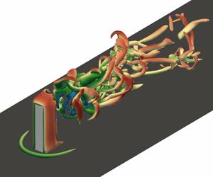
Figure 2. Instantaneous visualisation of the flow around a wall-mounted square cylinder considered here. The instantaneous vortical structures identified with the Q-criterion are shown with an isosurface of  $+10$ (scaled in terms of
  $U_\infty$ and
  $h$). Structures are coloured with the streamwise velocity, which ranges from
  $-0.79$ (dark blue) to
  $+1.23$ (dark red). Dark grey represents the bottom wall, whereas light grey indicates the building-like obstacle.
As we focus on the flow near the obstacle, the following region is extracted from the computational domain:  $-1\leq x/h \leq 5$,
  $0\leq y/h \leq 2$ and
  $-1.5\leq z/h \leq 1.5$. Using this reduced domain, we consider
  $10\,000$ three-dimensional instantaneous fields to perform the modal decompositions. The previous fields were spectrally interpolated from the original spectral element method mesh to another one with resolution
  $(N_x,N_y,N_z) = (300,100,150)$. All temporal parameters are expressed in convective time units, i.e. a ratio between the freestream velocity
  $U_\infty$ and the height of the obstacle
  $h$. The time step between snapshots is constant,
  ${\Delta t}_{s} = 0.005$, which yields a database spanning a total of 50 time units. This temporal resolution is enough to capture accurately the low- and high-frequency flow mechanisms identified in the literature (Martínez-Sánchez et al. Reference Martínez-Sánchez, Lazpita, Corrochano, Le Clainche, Hoyas and Vinuesa2023).
Some of the characteristics of the highly three-dimensional flow around a finite wall-mounted cylinder (Hunt et al. Reference Hunt, Abell, Peterka and Woo1978; Martinuzzi & Tropea Reference Martinuzzi and Tropea1993) are displayed in the instantaneous vortical structures of figure 2. Here, a horseshoe vortex extends around the two sides of the obstacle and into the wake. This vortex affects many of the flow structures around the cylinder, including the vortex-shedding mode, the shear-layer dynamics and the width of the wake (Rao, Sumner & Balachandar Reference Rao, Sumner and Balachandar2004; Vinuesa et al. Reference Vinuesa, Schlatter, Malm, Mavriplis and Henningson2015). As a result, this vortex also has an impact on the near-wake region and thus on the arch vortex formed on the leeward side of the obstacle (Wang et al. Reference Wang, Zhou, Chan and Lam2006; Wang & Zhou Reference Wang and Zhou2009). The large range of scales characteristic of turbulent flows in urban environments is also shown in figure 2, where the vortical structures within the wake exhibit a wide range of sizes and energy contents. The formation of the previous vortices and wake arises as a consequence of a fixed separation location prescribed by the sharp cylinder edges, whose associated separated shear layer can be noticed around every windward edge of the obstacle.
5. Reduced-order model for urban flows
Modal decomposition is a mathematical method for identifying essential energy and dynamic characteristics of fluid flows. These spatial features of the flow are known as spatial modes, and they are usually ranked in terms of the energy content levels or characteristic growth rates and frequencies driving the flow motion. These modal-decomposition techniques are generally used to create a low-dimensional coordinate system that reflects successfully the main characteristics of the flow. These structures are crucial not only for flow analysis, but also for reduced-order modelling and flow control. In this section, we discuss POD, which is used to generate a low-dimensional model of the flow around a finite square cylinder, representative of a simplified urban environment.
POD (Lumley Reference Lumley1967) is a modal-decomposition technique that has been employed traditionally in the fluid mechanics community. It seeks to decompose a set of data for a particular field variable into the fewest feasible modes (basis functions) while capturing the largest amount of energy. This process implies that POD modes are optimal in minimising the mean square error between the signal and its reconstructed representation. The low-dimensional latent space provided by the POD modes is attractive for interpreting the most energetic and dominant patterns within a given flow field. Let us consider a vector field  $\boldsymbol {q}(\boldsymbol {\xi },t)$, which may represent e.g. the velocity or the vorticity field, depending on a spatial vector
  $\boldsymbol {\xi }$ and time. In fluid flow applications, the temporal mean
  $\bar {\boldsymbol {q}}(\boldsymbol {\xi })$ is usually subtracted to analyse the fluctuating component of the field variable,
 \begin{equation} \boldsymbol x(t) = \boldsymbol{q}(\boldsymbol{\xi},t) - \bar{\boldsymbol{q}}(\boldsymbol{\xi}),\quad t = t_1,t_2,\ldots,t_k, \end{equation}
where  $\boldsymbol x(t)$ represents the fluctuating component of the vector data with its temporal mean removed. This representation emphasises the idea that the data vector
  $\boldsymbol x(t)$ is being considered as a collection of snapshots at different time instants
  $t_k$. If the
  $m$ snapshots are stacked into a matrix form, then we obtain the so-called snapshot matrix
  $\boldsymbol{\mathsf{X}}$:
 \begin{equation} \boldsymbol{\mathsf{X}} = [\boldsymbol x(t_1), \boldsymbol x(t_2),\ldots,\boldsymbol x(t_m)] \in \mathbb{R}^{J\times K}, \end{equation}
where  $J$ represents the number of points in
  $x$,
$x$,  $y$ and
  $z$. Note the similarity between this matrix and the definition provided in (2.7). In this case, we differentiate between the snapshot matrix
  $\boldsymbol{\mathsf{X}}\in \mathbb {R}^{J\times K}$, which is used for the modal-decomposition analysis, and the matrix
  $\boldsymbol {\mathcal {V}}\in \mathbb {R}^{n\times K}$, which is employed for the causality analysis. The objective of the POD analysis is to find the optimal basis to represent a given set of data
  $\boldsymbol x(t)$. This can be solved by finding the eigenvectors
  $\boldsymbol {\varPhi }_j$ and the eigenvalues
  $\lambda _j$ from
 \begin{equation} \boldsymbol{\mathsf{C}} \boldsymbol{\varPhi}_j = \lambda_j \boldsymbol{\varPhi}_j, \quad \boldsymbol{\varPhi}_j \in \mathbb{R}^{J}, \lambda_1\geq\cdots\geq\lambda_N\geq0, \end{equation}
where  $\boldsymbol{\mathsf{C}}$ denotes the covariance matrix of the input data, defined as
 \begin{equation} \boldsymbol{\mathsf{C}} = \sum_{i=1}^{K} \boldsymbol x(t_i)\,\boldsymbol x^\text{T}(t_i) = \boldsymbol{\mathsf{X}} \boldsymbol{\mathsf{X}} ^\text{T} \in \mathbb{R}^{J\times J}. \end{equation}
The size of this matrix depends on the spatial degrees of freedom of the problem. The POD modes are derived from the eigenvectors of (5.3), with the eigenvalues reflecting how well each eigenvector  $\boldsymbol {\varPhi }_j$ represents the original data in the
  $\ell _2$ sense. This allows us to categorise modes according to the amount of captured kinetic energy when the velocity fields are the data analysed, which enhances the assessment of the most prominent patterns in a given flow field.
We applied POD using the singular value decomposition method (Sirovich Reference Sirovich1987) on the database presented in § 4. Figure 3 shows the eigenvalues  $\lambda _m$, and the cumulative sum of eigenvalues
  $\sum _{i=1}^{i=m} \lambda _i$ normalised with the total energy of the eigenvalues
  $\sum _{i=1}^M \lambda _i$, where
  $m$ is used to identify the mode number. Note that using 10 linearly superposed modal functions,
  $30\,\%$ of the total energy can be represented, which is enough to characterise the large-scale structures driving the main dynamics in this type of flow (Xiao et al. Reference Xiao, Heaney, Mottet, Fang, Lin, Navon, Guo, Matar, Robins and Pain2019; Lazpita et al. Reference Lazpita, Martínez-Sánchez, Corrochano, Hoyas, Le Clainche and Vinuesa2022).

Figure 3. (a) Eigenvalues  $\lambda _m$ and (b) cumulative sum of the eigenvalues
  $\sum _{i=1}^{i=m} \lambda _i$, spectrum normalised with the total energy of the eigenvalues
  $\sum _{i=1}^M \lambda _i$. The mode number is denoted with
  $m$, and the solid red line represents the amount of energy contained within the first 10 modes.
Using this ten-mode model, we use the distinction of the flow mechanisms responsible for arch vortices in urban fluid flows performed in our previous work (Lazpita et al. Reference Lazpita, Martínez-Sánchez, Corrochano, Hoyas, Le Clainche and Vinuesa2022) to perform a similar classification. This division focuses on the identification of two main types of modes: vortex-generator modes (G) and vortex-breaker modes (B). The naming of these modes is purely associated with the shape of their associated structures, which is covered extensively in the works of Lazpita et al. (Reference Lazpita, Martínez-Sánchez, Corrochano, Hoyas, Le Clainche and Vinuesa2022) and Martínez-Sánchez et al. (Reference Martínez-Sánchez, Lazpita, Corrochano, Le Clainche, Hoyas and Vinuesa2023). The major structures and vortices are produced by the G modes; therefore, they are related to the mechanism that could create the horseshoe and arch vortices. Note that G modes typically exhibit a smaller energy content than B modes, and are found in the low-frequency region of the spectrum. The major flow structures could then be broken by the B modes, which are also responsible for the dynamics of the turbulent wake. In contrast to vortex-generators, B modes are present in the high-frequency region of the spectrum.
Since regions of strong recirculation have already been proved to increase concentration of passive scalars (Zhu et al. Reference Zhu, Wang, Wang and Wang2017), G modes, which are related to these prominent recirculation areas, could be related to high-pollutant-concentration areas (Monnier et al. Reference Monnier, Goudarzi, Vinuesa and Wark2018). Conversely, B modes could be connected with reduced-pollutant-concentration regions as they are responsible for the destruction mechanisms of the main spatio-temporal structures. Readers are referred to Lazpita et al. (Reference Lazpita, Martínez-Sánchez, Corrochano, Hoyas, Le Clainche and Vinuesa2022) and Martínez-Sánchez et al. (Reference Martínez-Sánchez, Lazpita, Corrochano, Le Clainche, Hoyas and Vinuesa2023) for a detailed discussion of the previous modes.
The three-dimensional structures characteristic of these two types of modes are represented in figure 4 for the present database. The vortex-breaker mode is shown in figure 4(a). This type of mode is represented by the first two POD modes shown in figure 3. Therefore, the vortex-breaking process is identified as the most energetically relevant mode present in the flow field. This result is in line with Lazpita et al. (Reference Lazpita, Martínez-Sánchez, Corrochano, Hoyas, Le Clainche and Vinuesa2022), who showed the agreement between the first two POD modes and the vortex-breaker modes identified using various modal-decomposition techniques, in terms of both frequency behaviour and spatial resemblance. Here, the streamwise turbulent wake consists of high-velocity coherent clusters on both sides of the obstacle wake, which are also related to the vortex-shedding phenomenon present in the flow past bluff bodies. This is also shown in the two-dimensional contours in figure 5, where the spatial structure of the two modes is observed to be the same, except for a shift in phase: they are both antisymmetric with respect to the  $z$-axis, and they represent the vortex-shedding phenomenon with identical frequency,
  $St = 0.45$. This is evidence that the modes represent a wave-like periodic structure of the flow. In fact, since the POD modes are real, two modes are needed to describe a flow structure travelling as a wave (Rempfer & Fasel Reference Rempfer and Fasel1994). Note that the POD method creates a low-dimensional coordinate system by linearly superposing orthogonal modes derived from data representing the turbulent flow. The POD modes capture the dominant features of the flow, some of which may arise as a result of the various underlying nonlinear interactions that characterise a turbulent flow. Consequently, there might be multiple modes with similar but not identical energy contributions. This could lead to minor variations in the magnitude of B modes, as illustrated in figure 3.

Figure 4. Three-dimensional isosurfaces of the streamwise velocity of (a) the vortex-breaker modes (B mode with  $a=b=0.3$), and (b) the vortex-generator modes (G mode with
  $a=0.5$ and
  $b=0.1$). Velocity values are normalised using the
  $L_{\infty }$-norm. Isovalues employed are given by
  $a U_{max}$ (red) and
  $b U_{min}$ (blue).
A similar analysis can be conducted using the third POD mode, whose associated structures are representative of G modes. In figure 4(b), we show that this mode is connected with the main vortex-generation mechanisms identified in Lazpita et al. (Reference Lazpita, Martínez-Sánchez, Corrochano, Hoyas, Le Clainche and Vinuesa2022). A large-scale streamwise structure, characteristic of this type of mode, is found just after the obstacle. This dome-like feature surrounds and interacts with the arch vortex by restricting its expansion (Martínez-Sánchez et al. Reference Martínez-Sánchez, Lazpita, Corrochano, Le Clainche, Hoyas and Vinuesa2023).
The rest of the modes are depicted in figure 5, where the spatial modes for the streamwise velocity fields are shown. An additional analysis of the temporal coefficients associated with these modes is conducted in the frequency domain through the fast Fourier transform method (Cooley & Tukey Reference Cooley and Tukey1965). This enables classifying the time coefficients associated with each spatial mode into low- and high-frequency phenomena, whose features are decisive for the vortex-generating and -breaking processes, respectively. Remarkably, these results show that the vortex-breaking process present in the first two most energetic modes is dominated by a single peak frequency  $St = 0.45$. Modes 3 and 4 are denoted as vortex-generator modes since their associated peak frequencies appear in the low-frequency region of the domain (
 $St =0.05$ and
  $0$, respectively) and their associated spatial structures, depicted in figures 4 and 5, show how a dome-like structure encloses the near-wake region of the flow. This behaviour is similar to that of the time-averaged field, thus it suggests that these modes could be the reason for the generation of such structures. Higher-order modes, i.e. modes 5–8, are also present in the low-frequency range of the spectrum. However, their flow features start to exhibit fluctuating features in the wake. These modes may then be regarded as G modes that are harmonics of the previous G modes with dominant frequencies
  $St=0.05$,
  $0.15$ and
  $0.2$. However, these modes are the result of nonlinear interactions, hence they can be regarded as hybrid (H) modes (which is the case for modes 9 and 10), whose interaction with each other is expected to be extracted from the causality analysis.

Figure 5. From upper left to lower right on two top rows: the first ten POD modes at  $y/h=0.75$ for the streamwise component of the velocity. Contours are normalised with the
  $L_\infty$-norm and range between
  $-1$ (blue) and
  $+1$ (red). Bottom: power spectral density (PSD) scaled with the Strouhal number
  $St=f h/U_\infty$ of the temporal coefficients associated with the corresponding POD modes, where
  $f$ is the characteristic frequency of each mode. The PSD is calculated using
  $N=8192$ (
 $2^{13}$) samples and window overlap
  $50\,\%$. Modes denoted as G* represent harmonics of vortex-generator modes.
6. Results and discussion
Using the previous ten-mode model, we apply the procedure discussed in § 3 to extract the causal interactions between the different flow mechanisms. To do that, we use the time coefficients associated with each of the POD modes, and we arrange them into a ten-component vector as in (2.7). Prior to the assessment of the causal results, the quantification of causality using (2.8) requires the definition of a certain fixed time delay,  $\Delta t$. In this study, we seek the time lag that produces the maximum causal inference between the variables, which we denote as
  ${\Delta t}_{max}$. Despite the inherent change in transfer-entropy behaviour for varying
  $\Delta t$ values, defining the summation of every causal relationship as a global measure, i.e.
  $\sum _{i,j} T_{i\rightarrow j}$, allows us to establish a sensible value for
  ${\Delta t}_{max}$. The evolution of this parameter is depicted in figure 6 as a function of the time lag, where
  ${\Delta t}$ is scaled in terms of the time step between snapshots
  ${\Delta t}_s$. Causalities are found to be maximum for time lag
  ${\Delta t}_{max} = 0.1$, which corresponds to a lag of
  $20$ snapshots. This value is comparable to the dynamics of the highest-frequency phenomena of the flow (Martínez-Sánchez et al. Reference Martínez-Sánchez, Lazpita, Corrochano, Le Clainche, Hoyas and Vinuesa2023) and represents
  $5\,\%$ of the period of the vortex-shedding modes.

Figure 6. Evolution of total causality  $\sum _{ij} T_{i\rightarrow j}$ as a function of time lag
  $\Delta t$. Note that
  $\Delta t$ is scaled in terms of the time step between snapshots,
  ${\Delta t}_s$, and total causality is normalised with the maximum value obtained for every
  $\Delta t$, i.e.
  $(\sum _{ij} T_{i\rightarrow j})_{max}=0.031$.
The transfer entropy is then calculated using (2.8) with  ${\Delta t}_{max}$ to obtain the cross-induced cause-and-effect interactions between the modes. The corresponding causal map is depicted in figure 7, where modes are labelled directly using the flow mechanism that they represent according to § 5. The map shows a very high causal inference between the first two modes compared to the rest of the relationships. The fact that these two modes are representative of the same flow mechanism but with a slight shift in phase makes their causal relationship evident. Causal inferences smaller in amplitude are also appreciated between B modes and the highest-order modes, i.e. modes 7–10. To better assess these interactions, the causal relationships between B modes are set to zero. The resulting causal map is illustrated in figure 7(b), where we observe the high causal connections
  $T_{2\rightarrow 10}$ and
  $T_{1\rightarrow 10}$. Vortex-breaker modes are then regarded as the most influential mechanism in higher-order modes, which we denoted as hybrid modes. However, vortex-generator modes (modes 3–6) do not have a direct causal inference over the rest of the modes.

Figure 7. Causal map for the ten-mode model of the studied database. Red-scale colours denote causality magnitude normalised with the  $L_\infty$-norm. Modes are labelled per their mechanism. The colour map in (b) is over-saturated to highlight the interactions of B modes with higher-order modes.
Similar conclusions can be drawn if we decide to consider only one B mode, since these modes represent the same flow mechanism, and their associated temporal evolution is equivalent but with a  ${\rm \pi} /2$ phase shift. This mechanism propagates as a travelling wave in a periodic fashion; therefore, two orthogonal modes in space are needed to represent its dynamics. This leads to the causal map shown in figure 8(a), where only one B mode can be noticed. This assumption produces effects similar to those found from modes 1 and 2 on higher-order modes. As seen in § 5, hybrid modes represent the interaction between B and G modes as a result of a varied range of frequencies found in the spectrum of their associated time coefficients. Therefore,
  $T_{B\rightarrow 10}$ reveals that the vortex-breaking mechanism drives the appearance of modes where shared features of both B and G modes are found.

Figure 8. Causal map for the ten-mode model of the studied database for (a) only one B mode, and (b) no B modes. Red-scale colours denote causality magnitude normalised with the  $L_\infty$-norm. Modes are labelled per their mechanism.
Figure 8(b) depicts the eight-mode causal map obtained as a result of removing the combined mode from the spectrum. Remarkably, a strong causal inference from mode 10 on mode 8,  $T_{10\rightarrow 8}$, is now appreciated. This proves that modes on which B modes have large influence also cause the appearance of modes whose frequency behaviour is harmonic of purely G modes. However, there is no sign that G modes are intimately related to any of the aforementioned mechanisms. A schematic diagram depicting the main causal interactions between each of the modes is presented in figure 9.

Figure 9. Diagram depicting the mutual inferences between modes due to the past states of the other modes. Only those significant causal interactions are represented. Two vortex-breaker (B) modes, two hybrid (H) modes and one vortex-generator (G) mode are shown, i.e. modes 1, 2, 10, 9 and 8, respectively.
Therefore, understanding the dynamics underlying the vortex-breaking mechanism in detail may be crucial for predicting the emergence of significant flow features in urban environments, such as the arch vortex. These findings also suggest that B modes are not only the most energetic modes in the flow field but also those responsible for the appearance of modes that relate to the generation of the primary vortical structures.
6.1. Influence of higher-order modes
We extend our analysis to investigate the causal influence of higher-order modes on the most energetic modes. The goal is to determine whether the large-scale structures of the flow, contained in the leading modes, exhibit strong causal relations with smaller-scale structures. To this end, we compute causal maps using a range of modes, from 10 to 40, and analyse the changes in the causal relations among them. Figure 10 illustrates the corresponding causal maps computed with different numbers of modes. The map computed with the first ten POD modes, shown in figure 10(a), corresponds to the case analysed in the previous section. This causal map highlights the strong causal inference observed between the most energetic modes of the system. As we increase the number of modes under consideration, we observe subtle changes in the causal relationships.

Figure 10. Causal map computed using (a) 10, (b) 20, (c) 30, and (d) 40 modes. Red-scale colours denote causality magnitude normalised with the  $L_\infty$-norm. Modes are labelled numerically in descending order according to their energy contribution to the system.
For instance, in the causal map computed with 20 modes (figure 10b), we still observe the strong causal trace of the large-scale structures. However, a higher causal inference is noted in this case from mode 17 to mode 18,  $T_{17\rightarrow 18}$. Furthermore, these two modes have a small impact on the first modes, similar in magnitude to the causal relation observed between them in figure 10(a). This observation supports the idea that smaller-scale structures can indeed have some influence over the more energetic modes, and should not be disregarded when assessing the prediction capabilities of the system or developing future control strategies. In the present study, the impact of smaller-scale structures on the leading modes is not substantial; however, this consideration might become more important in more complex systems, where these low-energy modes may play a prominent role.
When moving to the causal maps computed using 30 and 40 modes, as shown in figures 10(c) and 10(d), respectively, we can analyse the causal pattern of even-higher-order modes on the large-scale structures. The latter represents an ROM that accounts for more than  $60\,\%$ of the total energy of the flow. In these cases, we observe that the most significant causal relationships are found between the newly included modes in each map, such as
  $T_{27\rightarrow 29}$ in the thirty-mode map, and
  $T_{32\rightarrow 31}$ and
  $T_{39\rightarrow 36}$ in the forty-mode map. Interestingly, no traces of causal relations are left for the first POD modes, indicating that the leading modes are not affected when introducing these higher-order modes. This observation implies that only causal interactions are observed for the newly included modes, and suggests that it is sufficient to identify the most causal interactions between the large-scale structures of the flow using the ten-mode model. Therefore, our analysis supports the idea that the ten-mode model captures the essential dynamics and causal relations among the large-scale structures in the flow.
6.2. Time correlation between time coefficients
In this subsection, we compare the previous results with those obtained using a simplified approach for the quantification of causality, i.e. time correlation. This statistical metric describes the magnitude of the relationship between a given pair of variables without the directionality and asymmetry properties, which are required to estimate the causes and effects of events. Additionally, high correlation between the variables does not automatically mean that changes in one variable are caused by changes in the other variable. Despite this, it is interesting to compare the results from both approaches since a high causation emerges from some degree of correlation between variables, although the opposite does not hold. To assess correlation, the following expression is used:
 \begin{equation} {\mathsf{C}}_{ij}(\Delta t) = \frac{\langle{{\mathcal{V}_i}'(t), {\mathcal{V}_j}'(t+\Delta t)}\rangle}{\lVert{\mathcal{V}_i}'(t)\rVert\times \lVert{\mathcal{V}_j}'(t)\rVert}, \end{equation}
where  ${\mathcal {V}_i}'$ and
  ${\mathcal {V}_j}'$ represent the fluctuating signals
  ${\mathcal {V}_i}'={\mathcal {V}_i}-{\bar {\mathcal {V}}_i}$, and
  $\langle {\cdot } \rangle$ denotes the dot product operation taken over the whole time history. Note that using this expression, it is possible to deduce the symmetry property for correlation, i.e.
  ${\mathsf{C}}_{ij}(\Delta t) = {\mathsf{C}}_{ji}(-\Delta t)$.
Figure 11 depicts the effects of the variation of the time lag on the temporal cross-correlation between the time coefficients signals. Only those trends with a maximum value above  $0.4$ are represented. The main conclusion from these results is the high correlation observed between the first two modes. Remarkably, the correlation approaches value 1 when
  ${\Delta t}/T_{1,2} = 0.25$, where
  $T_{1,2}$ represents the period of the oscillations of the corresponding signals. This evolution confirms that the previous modes are representative of the same flow mechanism with a phase shift of
  ${\rm \pi} /2$ rad. This is in line with the causal relations observed in the previous subsection, where these modes represented the largest causation. A similar trend is also observed for modes 5 and 6, both G modes. In particular, a high correlation is observed for the previous modes when
  ${\mathsf{C}}_{1,2} = 0$. This means that the influence of B modes on the correlation between variables is predominant for low
  $\Delta t$ values, and it starts to decay for larger values of
  $\Delta t$. Conversely, for higher-order modes, their influence on the correlation with other variables starts to be more noticeable for large values of
  $\Delta t$ (when compared to B modes). This results in an increased interaction activity of modes 5 and 6, as correlation between modes 1 and 2 decays.

Figure 11. Time correlation between  $a_1\rightarrow a_2$ (red circles),
  $a_5\rightarrow a_6$ (black circles),
  $a_7\rightarrow a_5$ (squares) and
  $a_9\rightarrow a_8$ (triangles), where
  $a_m$ refers to the
  $m$th mode of the ROM. Note that
  $a_i\rightarrow a_j$ represents the expression for time correlation
  ${\mathsf{C}}_{ij}(\Delta t)$ in (6.1). Only those trends with a maximum value above
  $0.4$ are represented.
Furthermore, every signal discussed in this section exhibits a damped sinusoidal behaviour with a frequency pattern similar to that observed in figure 5: B modes are associated with high-frequency oscillations, whereas G modes are dominated by low-frequency ones. This means that depending on the employed time lag, the correlation between variables becomes reversed, which can be related to the fact that POD modes are based on a linear relationship. A similar conclusion was drawn from the transfer-entropy approach, where the modified values of the time lag produced different cause-and-effect interactions especially between the first two modes. Besides, damped waves are representative of poor correlations for increased values of the time lag, which hinders the extraction of both correlation and causation trends between variables.
7. Conclusions and further discussion
In the present work, we analysed the formation mechanisms of large-scale coherent structures in the flow around a wall-mounted square cylinder. We employed a database obtained by means of a direct numerical simulation to solve the flow around a single finite square cylinder of width-to-height ratio  $b/h=0.25$. Proper orthogonal decomposition (POD) was then applied to the previous database to generate a reduced-order model (ROM) with the ten most energetic modes, which represent
  $30\,\%$ of the overall energy of the flow. This model enables isolating the main mechanisms driving the dynamics of the flow in terms of space and time. The previous modes were classified as vortex-generator (G) and vortex-breaker (B) modes as a result of their spatial features and associated frequency behaviour. We investigated the causal interactions between these mechanisms, with the objective of understanding the origin and evolution of the various three-dimensional topological patterns that precede the formation of the well-known vortical structures found in this type of flow. To that end, we applied conditional transfer entropy over the time coefficients associated with each of the POD modes. This approach is based on an information-theoretical quantity that quantifies the amount of information flowing from the past state of one variable to another. In particular, we identified B modes as the most causative modes over higher-order modes, which we denoted as hybrid (H) modes due to their shared features with B and G modes. The cases in which B modes have large influence, i.e. H modes, were also found to drive the appearance of modes whose frequency behaviour is harmonic of purely G modes. Also, no significant causal relationships were observed for G modes, a fact that highlights the importance of understanding the underlying dynamics of B mechanisms to predict the emergence of significant flow features in urban environments. These results are in line with the previous classification of modes and shed light on new possibilities for future urban-flow control research. This includes active flow control targeting the modes responsible for generation of large-scale structures that may increase pollutant concentration in cities. Furthermore, the goal of the framework presented in this study for the estimation of causal interactions is to highlight the structures that are most causal over the rest of the system modes. Therefore, these structures should be the core of a posterior reduced-order-modelling process, which can be posed as a problem of conservation of information (Lozano-Durán & Arranz Reference Lozano-Durán and Arranz2022).
The tool employed for the quantification of causality was validated previously through the analysis of the causal relations present in a low-dimensional model for turbulent shear flows developed by Moehlis et al. (Reference Moehlis, Faisst and Eckhardt2004). We identified three main causal relations, which were related to the lift-up mechanism, the generation of streamwise rolls, and the mean-flow instability in the spanwise direction. All of them were in accordance with the results reported by Lozano-Durán et al. (Reference Lozano-Durán, Bae and Encinar2020) for turbulent channel flows.
In concluding our work, we discuss the main limitations of the methods employed and their potential applicability to more complex flows. Our ROM with ten linearly superposed modes successfully represents the large-scale structures of the flow. It is important to mention that in the context of the present work, the impact of the truncation on the temporal dynamics does not appear to significantly affect the causality analysis. However, in more complex flows, this truncation may be problematic, thus being able to develop more compact ROMs (Solera-Rico et al. Reference Solera-Rico, Vila, Gómez, Wang, Almashjary, Dawson and Vinuesa2023) might be necessary. Based on previous studies (Lazpita et al. Reference Lazpita, Martínez-Sánchez, Corrochano, Hoyas, Le Clainche and Vinuesa2022), we proved that the modes not included in the current ROM likely have a minimal impact on the overall causal inferences of higher-order modes on the large-scale structures of the flow. Nevertheless, it is essential to verify these results with other models that include a larger number of modes. Alternative modal-decomposition techniques, such as dynamic mode decomposition or Koopman mode decomposition, could also be explored to efficiently represent the global flow dynamics. Our energy-based truncation method is suitable for capturing large-scale structures in the wake of a finite square cylinder. However, in more complex systems, such as jets, aerofoils, wakes and mixing layers, the energy content of structures may not be an ideal criterion for truncation. In these cases, feedback mechanisms resulting from upstream pressure propagation or compressible acoustic effects might play a crucial role. One possible approach is to employ ROMs based on resolvent analysis or nonlinear Galerkin methods, which can better account for these feedback mechanisms. Regardless of the choice of ROM or truncation method, our causality analysis remains valid as long as the temporal history of the modal components is available. This reinforces the versatility of our methodology, which can be applied to various flow situations and modal decomposition techniques, provided that the essential temporal information is accessible.
Moreover, the identification of causal interactions between variables remains an ongoing challenge. Appropriate metrics have to be defined, especially given the vast number of parameters whose selection is critical in the resulting causality. In particular, typical operationalisations of causality estimators are based on a strong assumption that each point in the time series of effects is influenced by a combination of other time series with a fixed time lag. This is usually not the case in real-life systems, therefore a clear generalisation is needed to relax the above assumption. More importantly, the notion of causality followed here is based on Shannon statistical entropy and should therefore be interpreted as a probabilistic measure of causality and not as the measurements of individual events.
Funding
R.V. acknowledges financial support by the G. Gustafsson and Lundeqvist foundations, as well as from ERC grant no. 2021-CoG-101043998, DEEPCONTROL. A.S. acknowledges support from the NSF CAREER, USA grant no. 1554033 to the Illinois Institute of Technology. S.L.C. acknowledges the grant PID2020-114173RB-I00 funded by MCIN/AEI/10.13039/501100011033. E.L. acknowledges T. and J. Morel for their generosity, support, and the creation of the Morel Fellowship, which allowed this work to occur.
Declaration of interests
The authors report no conflict of interest.
Data availability statement
All the codes and databases used in this study are available in the following repository: https://github.com/KTH-FlowAI/causality-urban-flows.
Appendix A. Overview of low-dimensional model for near-wall turbulence
In this appendix, we provide an overview of the low-dimensional model for turbulent shear flows developed by Moehlis et al. (Reference Moehlis, Faisst and Eckhardt2004). The model is based on Fourier modes and describes the flow between two free-slip walls subjected to a sinusoidal body force. The essential elements of the model are nine modes  $\boldsymbol {v}_j(\boldsymbol {x})$, where
  $\boldsymbol {v}_1$ represents the basic mean velocity profile,
  $\boldsymbol {v}_2$ the streaks,
  $\boldsymbol {v}_3$ the downstream vortex,
  $\boldsymbol {v}_4$ and
  $\boldsymbol {v}_5$ the spanwise flows,
  $\boldsymbol {v}_6$ and
  $\boldsymbol {v}_7$ the normal vortex modes,
  $\boldsymbol {v}_8$ a three-dimensional mode, and
  $\boldsymbol {v}_9$ the modification of the basic profile. All but one of the modes were already introduced by the eight-mode model proposed by Waleffe (Reference Waleffe1997) for sinusoidal shear flow turbulence, with some additional couplings between modes included in the case employed in this work. An extra mode is also introduced in the model of Moehlis et al. (Reference Moehlis, Faisst and Eckhardt2004) to account for the modification of the structure of the mean velocity profile, over which turbulent fluctuations are known to have a significant impact. The instantaneous velocity fields can be obtained by superposing the previous nine modes as
 \begin{equation} \boldsymbol{u}(\boldsymbol{x},t) := \sum_{j=1}^9 a_j(t)\, \boldsymbol{v}_j(\boldsymbol{x}), \end{equation}
where the spatial coordinates are denoted by  $\boldsymbol {x}$, and
  $t$ represents the time. The Galerkin projection of the Navier–Stokes equations can then be applied onto this subspace to obtain a system of nine ordinary differential equations (ODEs) in time. Each ODE term exhibits a linear term, several nonlinear terms (including the interactions between modes under the shape
  $q_k(t) = a_i(t)\,a_j(t)$), and a constant. Hence they can generally be written as
 \begin{equation} \frac{{\rm d} \boldsymbol{a}(t)}{{\rm d}t} = \boldsymbol{\mathsf{L}}\,\boldsymbol{a}(t) + \boldsymbol{\mathsf{N}}\,\boldsymbol{q}(t) + \boldsymbol{c}, \end{equation}
where  $\boldsymbol {a}\in \mathbb {R}^n$ represents the vector of mode amplitudes,
  $\boldsymbol {q}\in \mathbb {R}^m$ is the vector of nonlinear processes,
  $\boldsymbol{\mathsf{L}}\in \mathbb {R}^{n\times n}$ and
  $\boldsymbol{\mathsf{N}}\in \mathbb {R}^{m\times n}$ are the matrices of coefficients for the linear and nonlinear terms, respectively, and
  $\boldsymbol {c}\in \mathbb {R}^{n}$ is the vector of constants. The Reynolds number is defined as a function of the channel full height
  $2\ell$ and the laminar velocity
  $U_0$ at distance
  $\ell /2$ from the top wall. The model used here corresponds to
  $Re = 400$, where
  $\ell$ and
  $U_0$ are used as length and velocity scales, respectively. The domain size is
  ${\mathsf{L}}_x=4{\rm \pi}$,
  ${\mathsf{L}}_y=2$ and
  ${\mathsf{L}}_z=2{\rm \pi}$, where
  $x$,
$x$,  $y$ and
  $z$ denote the streamwise, wall-normal and spanwise directions, respectively. Over this domain, the ODE model was used to obtain 600 sets of time series of the nine amplitudes, each with time span
  $4000$ time units and time step
  $0.01$ time units. These sets of time series are the result of introducing a random perturbation to
  $a_4$.
Appendix B. Assessment of statistical convergence
To provide a visual impression of the statistical convergence of the causal maps in figure 7, we depict in figure 12 the values of causality magnitude using the complete dataset (figures 12(a) and 12(c), equivalent to figure 7 in the main text), and a reduced dataset by considering half of the temporal history of the signals (figures 12(b) and 12(d)). The results indicate that variations in the causality magnitude of the most intense interactions are below  $15\,\%$. Not surprisingly, a higher causal inference is observed in the reduced dataset for the first mode over both hybrid modes when compared to the complete dataset. As these modes are representative of the same flow mechanism, this transition in causality is expected from the different temporal datasets. This means that the causal activity of mode 1 (shifted in phase with respect to mode 2) is larger in the half the data considered for this analysis, whereas mode 2 increases its activity in the second half of the temporal data. Despite this, we can conclude that the temporal data employed for the urban-flow model are sufficient, since these variations remain fenced within a maximum of
  $15\,\%$ difference when considering half of the available temporal data, and yielded identical physical conclusions.

Figure 12. Causal map computed using (a,c) the complete temporal dataset, and (b,d) half of the temporal history of the dataset. Red-scale colours denote causality magnitude normalised with the  $L_\infty$-norm. The colour maps in (c) and (d) are over-saturated to highlight the interactions of B modes with higher-order modes.
In this appendix, we also present the convergence study that was performed to verify that the 600 sequences employed in the causal map of the near-wall cycle of turbulence (figure 1) were sufficient. In this case, as the differing initial conditions employed for generating each of the 600 sequences resulted in different instances of the model, a convergence study is needed to verify whether more sequences would be required to obtain an accurate transfer-entropy calculation of the Moehlis et al. (Reference Moehlis, Faisst and Eckhardt2004) model. This was performed by assessing the average  $\ell _2$ difference between five sets of
  $m$ causal maps. The completed procedure resulted in the convergence plot shown in figure 13. It clearly indicates that by averaging the resulting transfer entropy over 120 sequences, the average
  $\ell _2$ difference between causal maps is below
  $10\,\%$ across all causal pairings. Given that there are 72 unique causal pairings in a single
  $9\times 9$ heat map, dividing the
  $10\,\%$ difference across the entire matrix results in a
  $0.14\,\%$ difference on average across each individual pairing. Therefore, it can be concluded that the 600 sequences were more than sufficient to obtain a representative causal heat map of the Moehlis model under the conditions used for its simulation.

Figure 13. Convergence plot of transfer-entropy results for the low-dimensional model of the near-wall cycle of turbulence using the  $k$-nearest-neighbour entropy estimator on all 600 sequences of the model. Convergence was assessed by creating five sets of
  $m$ sequences averaged with each other, and calculating the average
  $\ell _2$ difference between each of the heat maps, which means that
  $m=120$ represents the complete dataset.


 Open access