


1. Introduction
Since fluid motion on large and intermediate scales is directly resolved in a large eddy simulation (LES) (Meneveau Reference Meneveau2000; Lesieur, Metais & Comte Reference Lesieur, Metais and Comte2005; Sagaut Reference Sagaut2006), the LES framework is often considered to be the most appropriate for computational fluid dynamics (CFD) research on turbulent flows of practical relevance. However, since LES deals with velocity and scalar fields that are averaged over scales smaller than a filter size, subgrid-scale (SGS) motion is not resolved, but filtered out. Accordingly, both characteristics of this motion and its influence on the resolved fields must be modelled, with existing SGS models being challenged by specific phenomena.
For instance, according to the classical theory of locally homogeneous and isotropic turbulence in incompressible flows (Kolmogorov Reference Kolmogorov1941; Monin & Yaglom Reference Monin and Yaglom1975; Frisch Reference Frisch1995), both turbulent kinetic energy and mixture non-uniformities are transferred (on average) from large scales, where the energy and non-uniformities are generated, to small scales via the turbulence cascade (Richardson Reference Richardson1922) and are dissipated due to molecular viscosity and diffusion, respectively, at the smallest scales. However, an instantaneous local SGS energy flux obtained by filtering a turbulent velocity field fluctuates randomly and may be in the opposite direction of the mean energy flux (Leslie & Quarini Reference Leslie and Quarini1979; Piomelli et al. Reference Piomelli, Cabot, Moin and Lee1991; Borue & Orszag Reference Borue and Orszag1998; Cerutti & Meneveau Reference Cerutti and Meneveau1998). This phenomenon is known as backscatter of kinetic energy. A similar phenomenon has also been discussed in the literature of turbulent mixing (Jiménez, Valiño & Dopazo Reference Jiménez, Valiño and Dopazo2001; Marstorp, Brethouwer & Johansson Reference Marstorp, Brethouwer and Johansson2007).
While the classical forward cascade statistically overwhelms backscatter in many turbulent flows (Piomelli et al. Reference Piomelli, Cabot, Moin and Lee1991; Jiménez et al. Reference Jiménez, Valiño and Dopazo2001; Kobayashi Reference Kobayashi2005; Marstorp et al. Reference Marstorp, Brethouwer and Johansson2007), there are flows where backscatter definitely plays an important role and inverse cascade (i.e. transfer of kinetic energy or mixture non-uniformities from smaller to larger scales) can be statistically significant. As far as mixing in a non-reacting turbulent flow is concerned, three different physical scenarios are discussed in detail in a recent review article by Alexakis & Biferale (Reference Alexakis and Biferale2018). These are (i) a passive scalar in incompressible turbulence, with the forward cascade dominating in this case, (ii) a passive scalar in compressible turbulence, with cascade being reversed at a sufficiently high degree of compressibility (Chertkov, Kolokolov & Vergassola Reference Chertkov, Kolokolov and Vergassola1998; Gawedzki & Vergassola Reference Gawedzki and Vergassola2000), and (iii) an active scalar, which affects the flow (e.g. temperature differences yield buoyancy forces). As concluded by Alexakis & Biferale (Reference Alexakis and Biferale2018, p. 70), ‘it is not possible to make any general conclusions about’ cascade direction in case (iii). The direction depends on details such as length scales associated with scalar injection and significant influence of the scalar on the flow.
Both scenarios (ii) and (iii) are relevant to premixed turbulent flames, where heat release, density variations, dilatation and chemical reactions are confined to spatial scales, which are on the order of laminar flame thickness, and, thus, are substantially smaller than scales of large turbulent eddies, but are often larger than or comparable with Kolmogorov length scale. Therefore, in many premixed turbulent flames, active scalar fields evolve in a highly compressible flow (e.g. mean dilatation is positive, contrary to a typical non-reacting compressible flow, and is sufficiently large when compared with velocity gradients in the incoming turbulence), with injection of kinetic energy and mixture non-uniformities occurring at small scales and being well correlated (confined to the same zones). Accordingly, the phenomenon of backscatter of SGS kinetic energy in flames has received extensive attention over the past years (Kolla et al. Reference Kolla, Hawkes, Kerstein, Swaminathan and Chen2014; Ranjan et al. Reference Ranjan, Muralidharan, Nagaoka and Menon2016; Towery et al. Reference Towery, Poludnenko, Urzay, O'Brien, Ihme and Hamlington2016; O'Brien et al. Reference O'Brien, Towery, Hamlington, Ihme, Poludnenko and Urzay2017; Kim et al. Reference Kim, Bassenne, Towery, Hamlington, Poludnenko and Urzay2018; Ranjan & Menon Reference Ranjan and Menon2018; Ahmed, Chakraborty & Klein Reference Ahmed, Chakraborty and Klein2019; Kazbekov & Steinberg Reference Kazbekov and Steinberg2021, Reference Kazbekov and Steinberg2023; MacArt & Mueller Reference MacArt and Mueller2021; Datta, Mathew & Hemchandra Reference Datta, Mathew and Hemchandra2022; Qian et al. Reference Qian, Lu, Zou and Yao2022). On the contrary, backscatter of SGS scalar variance in turbulent flames has rarely been explored (Ranjan et al. Reference Ranjan, Muralidharan, Nagaoka and Menon2016), in spite of the fact that, as noted in the next section, this phenomenon is closely linked with SGS counter-gradient scalar transport, which is often addressed in LES of premixed turbulent combustion (Boger et al. Reference Boger, Veynante, Boughanem and Trouve1998; Weller et al. Reference Weller, Tabor, Gosman and Fureby1998; Tullis & Cant Reference Tullis and Cant2002; Richard et al. Reference Richard, Colin, Vermorel, Benkenida, Angelberger and Veynante2007; Pfadler et al. Reference Pfadler, Dinkelacker, Beyrau and Leipertz2009; Lecocq et al. Reference Lecocq, Richard, Colin and Vervisch2010; Klein, Chakraborty & Gao Reference Klein, Chakraborty and Gao2016; Klein et al. Reference Klein, Kasten, Chakraborty, Mukhadiyev and Im2018).
It is noted that backscatter of SGS scalar variance is of importance not only for LES of turbulent mixing and combustion, but also for general understanding of physical mechanisms of flame-turbulence interaction. Indeed, following the pioneering work by Damköhler (Reference Damköhler1940), the influence of intense small-scale turbulence on a premixed flame is commonly reduced to turbulent mixing (Sabelnikov, Yu & Lipatnikov Reference Sabelnikov, Yu and Lipatnikov2019; Sabelnikov & Lipatnikov Reference Sabelnikov and Lipatnikov2021). However, under conditions associated with backscatter of SGS scalar variance, such a simplification may not be sufficient and the influence of combustion on scalar fluctuation cascade should also be taken into account.
Accordingly, the present communication aims at exploring the physics of combustion-induced backscatter of SGS scalar variance by investigating not only scalar transport by the entire turbulent velocity fields obtained in earlier direct numerical simulations (DNS), but also separate contributions to the scalar transport from solenoidal and potential velocity fields yielded by Helmholtz–Hodge decomposition (HHD) (Chorin & Marsden Reference Chorin and Marsden1993) of the entire velocity fields. In the next section, mathematical background is summarized. The DNS attributes and numerical diagnostics are addressed in § 3. Subsequently, the obtained results are reported and discussed in § 4, followed by conclusions.
2. Background
A common practice of premixed turbulent combustion modelling consists in characterizing mixture state in a flame with a single scalar quantity  $c$, which monotonically varies from zero in fresh reactants to unity in equilibrium combustion products and is known as the combustion progress variable (Bilger et al. Reference Bilger, Pope, Bray and Driscoll2005; Poinsot & Veynante Reference Poinsot and Veynante2005). Starting from the continuity equation and the following standard transport equation for
  $c$,
$c$,
 \begin{equation} \rho \frac{\partial c}{\partial t} + \rho \boldsymbol{u} \boldsymbol{\cdot} \boldsymbol{\nabla} c + \boldsymbol{\nabla}\boldsymbol{\cdot} \boldsymbol{J} = \rho \dot{\omega}, \end{equation}
one can easily arrive at the following well-known transport equations for filtered (resolved) combustion progress variable  $\tilde {c}$,
 \begin{equation} \bar{\rho} \frac{\partial \tilde{c}}{\partial t} + \bar{\rho} \tilde{\boldsymbol{u}} \boldsymbol{\cdot}\boldsymbol{\nabla} \tilde{c}+ \boldsymbol{\nabla}\boldsymbol{\cdot} \bar{\boldsymbol{J}} = \bar{\rho} \tilde{\dot{\omega}} - \boldsymbol{\nabla} \boldsymbol{\cdot} \left(\bar{\rho} \tilde{\boldsymbol{f}}\right) \end{equation}
and for filtered ‘scalar energy’  $\tilde {c}^2$,
 \begin{equation} \bar{\rho} \frac{\partial \tilde{c}^2}{\partial t} + \bar{\rho} \tilde{\boldsymbol{u}} \boldsymbol{\cdot}\boldsymbol{\nabla} \tilde{c}^2+ 2 \boldsymbol{\nabla}\boldsymbol{\cdot} \left( \bar{\rho} \tilde{c} \tilde{\boldsymbol{f}} \right)={-} G + 2 \tilde{c} \bar{\rho} \tilde{\dot{\omega}} - 2 \tilde{c} \boldsymbol{\nabla}\boldsymbol{\cdot} \bar{\boldsymbol{J}}. \end{equation}
Here,  $\bar {q}$ and
  $\tilde {q} \equiv \overline{\rho q}/\bar {\rho }$ designate filtered and Favre-filtered, respectively, values of the quantity
  $q$;
$q$;  $t$ is time;
  $\rho$ is density;
  $\boldsymbol {u}$ is flow velocity vector;
  $\boldsymbol {J}$ is molecular flux of
  $c$;
$c$;  $\dot {\omega }$ is rate of product creation;
  $\tilde {\boldsymbol {f}} = \widetilde {\boldsymbol {u} c}-\tilde {\boldsymbol {u}} \tilde {c}$ is SGS flux of
  $c$; and
  $G \equiv - 2 \bar {\rho } \tilde {\boldsymbol {f}} \boldsymbol {\cdot }\boldsymbol {\nabla } \tilde {c}$ describes inter-scale flux of the scalar energy from resolved to subgrid scales (if
  $G>0$) or in reverse direction (if
  $G<0$). Thus, counter-gradient SGS scalar transport, i.e. a positive product of the vectors
  $\tilde {\boldsymbol {f}}$ and
  $\boldsymbol {\nabla } \tilde {c}$, is a necessary condition for backscatter of SGS scalar variance. Note that (i) a transport equation for SGS scalar variance
  $\sigma _c \equiv \widetilde {c^2} - \tilde {c}^2$ involves the same term
  $G$, but with the opposite sign.
The focus of the present study is placed on the physics of the influence of combustion on the inter-scale flux  $G$ and, in particular, on its sign. For this purpose, it is essential to split the velocity field into potential and solenoidal components, because the former (latter) component does (does not, respectively) involve combustion-induced dilatation. Accordingly, HHD has been applied to the velocity fields, i.e.
 \begin{equation} \boldsymbol{u}(\boldsymbol{x},t)=\boldsymbol{u}_s(\boldsymbol{x},t)+\boldsymbol{u}_p(\boldsymbol{x},t);\quad \boldsymbol{\nabla}\boldsymbol{\cdot} \boldsymbol{u}_s=0;\quad \boldsymbol{\nabla} \times \boldsymbol{u}_p=0. \end{equation}
The solenoidal velocity  $\boldsymbol {u}_s(\boldsymbol {x},t)$ is divergence-free and arises due to shear and a rigid-body rotation. The potential velocity
  $\boldsymbol {u}_p(\boldsymbol {x},t)$ is curl-free and stems from dilatation due to thermal expansion. HHD offers the opportunity to directly explore potential motion due to thermal expansion and investigate the influence of this motion on the scalar cascade.
3. DNS attributes
Since simulations whose data are analysed in the present paper were already discussed earlier (Im et al. Reference Im, Arias, Chaudhuri and Uranakara2016; Uranakara et al. Reference Uranakara, Chaudhuri, Dave, Arias and Im2016; Wacks et al. Reference Wacks, Chakraborty, Klein, Arias and Im2016; Klein et al. Reference Klein, Kasten, Chakraborty, Mukhadiyev and Im2018; Manias et al. Reference Manias, Tingas, Hernández Pérez, Galassi, Ciottoli, Valorani and Im2019; Klein et al. Reference Klein, Herbert, Kosaka, Böhm, Dreizler, Chakraborty, Papapostolou, Im and Hasslberger2020; Lipatnikov et al. Reference Lipatnikov, Sabelnikov, Hernández-Pérez, Song and Im2020, Reference Lipatnikov, Sabelnikov, Hernández-Pérez, Song and Im2021; Sabelnikov et al. Reference Sabelnikov, Lipatnikov, Nishiki, Dave, Hernández-Pérez, Song and Im2021c, Reference Sabelnikov, Lipatnikov, Nikitin, Hernández-Pérez and Im2022a,Reference Sabelnikov, Lipatnikov, Nikitin, Hernández-Pérez and Imb), only a brief summary of the DNS attributes is given below.
Unconfined statistically one-dimensional and planar, lean (the equivalence ratio  ${\varPhi =0.7}$) hydrogen–air turbulent flames were studied by (i) adopting a detailed (9 species, 23 reversible reactions) chemical mechanism (Burke et al. Reference Burke, Chaos, Ju, Dryer and Klippenstein2012) with the mixture-averaged transport model and (ii) numerically solving unsteady three-dimensional governing equations, written in compressible form. Note that while differential diffusion effects are well known to be highly pronounced in very lean hydrogen–air flames and to significantly increase turbulent burning velocity, as reviewed elsewhere (Lipatnikov & Chomiak Reference Lipatnikov and Chomiak2005), differential diffusion was shown (Chen & Im Reference Chen and Im2000; Im & Chen Reference Im and Chen2002) to weakly affect a mean bulk burning rate at
  $\varPhi =0.7$ used in the present study.
Along the flame propagation direction, inflow and outflow characteristic boundary conditions were set. Other boundaries were periodic. Divergence-free, isotropic, homogeneous turbulent velocity field was generated in a box using a pseudo spectral method (Rogallo Reference Rogallo1981) and adopting the Passot–Pouquet spectrum (Passot & Pouquet Reference Passot and Pouquet1987). Subsequently, the field was injected through the left boundary and decayed along the mean flow direction ( $x$-axis). With the intention to explore corrugated flamelet and thickened flame combustion regimes (Im et al. Reference Im, Arias, Chaudhuri and Uranakara2016), the spectra were set using the same length scale
  $L_T=5$ mm of the most energetic eddies, but two different r.m.s. velocities
  $u'_0=0.95$ and 6.8 m s
 $^{-1}$ in cases A and B, respectively. The turbulent Reynolds number
  ${\textit {Re}}_T=u'_0 L_T/\nu _u=227$ and 1623, respectively, where
  $\nu_{u}$ is the kinematic viscosity of unburned gas. Since the injected turbulent velocity field evolved along the
  $x$-direction (Sabelnikov et al. Reference Sabelnikov, Lipatnikov, Nikitin, Hernández-Pérez and Im2022b, figure 1), the flames interacted with turbulence whose characteristics, e.g. the r.m.s. velocity and integral length scale reported in table 1, depended on, but differed from
  $u'_0$ and
  $L_T$, respectively, with the difference magnitude being case-dependent.
Table 1. Flame characteristics.

Major characteristics of two investigated cases are reported in table 1, where the laminar flame speed  $S_L=1.36$ m s
 $^{-1}$ and thickness
  $\delta _L=(T_b-T_u)/\max \{|{\rm d} T/{{\rm d}\kern0.06em x}|\}=0.36$ mm have been computed adopting the same chemical mechanism (Burke et al. Reference Burke, Chaos, Ju, Dryer and Klippenstein2012);
  $T$ is the temperature; subscript
  $u$ or
  $b$ refers to unburned or burned mixture, respectively. The r.m.s. velocity
  $u'=\sqrt {2 \langle k \rangle /3}$, the turbulent kinetic energy
  $\langle k \rangle = \langle u'_k u'_k \rangle /2$, its dissipation rate
  $\langle \varepsilon \rangle = 2 \nu _u \langle S_{jk} S_{jk} \rangle$, the integral length scale
  $L_{k \varepsilon }=\langle k \rangle ^{3/2}/\langle \varepsilon \rangle$, Damköhler number
  $Da=L_{k \varepsilon } S_L/(u' \delta _L)$, and the Kolmogorov length scale
  $\eta _K=(\nu _u^3/\langle \varepsilon \rangle )^{1/4}$ are obtained by averaging over the transverse plane where the plane-averaged fuel-based combustion progress variable
  $\langle c \rangle (x,t)=0.05$, followed by time-averaging;
  $u'_k(\boldsymbol {x},t)$ designates fluctuation of the
  $k$th component of the local velocity vector;
  $S_{jk} = (\partial u_j/\partial x_k + \partial u_k/\partial x_j)/2$ is the rate-of-strain tensor;
  $\langle q \rangle$ designates time- and transverse-averaged value of the quantity
  $q$; and summation convention applies to repeated indexes.
The velocity field  $\boldsymbol {u}(\boldsymbol {x},t)$ yielded by the DNS is decomposed into solenoidal and potential components,
  $\boldsymbol {u}_s(\boldsymbol {x},t)$ and
  $\boldsymbol {u}_p(\boldsymbol {x},t)$, respectively, adopting numerical methods applied earlier to velocity fields obtained from weakly turbulent single-step chemistry flames (Sabelnikov et al. Reference Sabelnikov, Lipatnikov, Nikitin, Nishiki and Hasegawa2021a,Reference Sabelnikov, Lipatnikov, Nikitin, Nishiki and Hasegawab) and from the two present flames A and B (Sabelnikov et al. Reference Sabelnikov, Lipatnikov, Nikitin, Hernández-Pérez and Im2022a,Reference Sabelnikov, Lipatnikov, Nikitin, Hernández-Pérez and Imb). The methods are discussed in detail elsewhere (Sabelnikov et al. Reference Sabelnikov, Lipatnikov, Nikitin, Nishiki and Hasegawa2021a, Reference Sabelnikov, Lipatnikov, Nikitin, Hernández-Pérez and Im2022a). Solenoidal and potential SGS scalar fluxes and inter-scale fluxes were evaluated as follows:
 \begin{align} \tilde{\boldsymbol{f}}_s = \widetilde{\boldsymbol{u}_s c}-\tilde{\boldsymbol{u}}_s \tilde{c};\quad \tilde{\boldsymbol{f}}_p = \widetilde{\boldsymbol{u}_p c}-\tilde{\boldsymbol{u}}_p \tilde{c};\quad G_s ={-} 2 \bar{\rho} \widetilde{\boldsymbol{f}_s} \boldsymbol{\cdot}\boldsymbol{\nabla} \tilde{c};\quad G_p ={-} 2 \bar{\rho} \widetilde{\boldsymbol{f}_p} \boldsymbol{\cdot}\boldsymbol{\nabla} \tilde{c}. \end{align}
Since all these equations are linear with respect to velocity,  $\boldsymbol {f}=\boldsymbol {f}_s+\boldsymbol {f}_p$ and
  ${G=G_s+G_p}$.
The computed fields of  $\rho (\boldsymbol {x},t)$,
  $c(\boldsymbol {x},t)$,
  $\boldsymbol {u}(\boldsymbol {x},t)$,
  $\boldsymbol {u}_s(\boldsymbol {x},t)$ and
  $\boldsymbol {u}_p(\boldsymbol {x},t)$, sampled by processing six snapshots (
 $t/t_e=0.57$, 0.67, 0.77, 0.86, 0.96 and 1.05 in case A or
  $t/t_e=4.1$, 4.8, 5.5, 6.2, 6.8 and 7.5 in case B, where
  $t_e=L_T/u'_0$) were filtered adopting top-hat (box) filters of three different sizes
  $\varDelta /\delta _L=0.43$, 0.87 and 1.74, with mass-weighted (Favre) filtering being applied to all these quantities with the exception of density. The smallest and largest filter widths, normalized using
  $\eta _K$ or
  $L_{k \varepsilon }$, are reported in table 1. The combustion progress variable was evaluated using fuel mass fraction
  $Y_F$, i.e.
  $c=(Y_F-Y_{f,u})/(Y_{f,b}-Y_{f,u})$. Quantities conditioned to the normalized filtered dilatation
  $\varTheta = \delta _L \boldsymbol {\nabla } \boldsymbol {\cdot } \tilde {\boldsymbol {u}}/(\tau S_L)$ were sampled by dividing an interval of
  $\varTheta \in [-0.2, 1.3]$ in 100 bins from the entire computational domain and at all instants. Here,
  $\tau =(\rho _u/\rho _b)-1$. Probability density functions (PDFs) for various quantities were also sampled using 100 bins from the entire computational domain and at all instants.
4. Results and discussion
Figure 1 shows that time- and transverse-averaged inter-scale flux  $\langle G \rangle (x)$ (see black solid lines) is negative for different filters in both flames, i.e. backscatter of SGS scalar variance is well pronounced in each studied case. Even the transverse-averaged counterpart of the filtered
  $\langle G \rangle$ is negative under the present DNS conditions (not shown for brevity). The backscatter magnitude
  $|\langle G \rangle |(x)$ and the magnitude of SGS scalar flux (see figure 3, which will be discussed later) peak in the middle of the flame brush, where the probability of finding thin instantaneous flames is the highest and these flames contribute the most to filtered values of quantities that vanish in reactants and products (e.g.
  $\boldsymbol {\nabla } c$). Moreover, the backscatter magnitude is increased with increasing
  $\varDelta$, because the use of a narrower filter results in decreasing subgrid fluctuations and, in particular,
  $|\tilde {\boldsymbol {f}}|$ and
  $|G|$ (these fluctuations and fluxes vanish at
  $\varDelta \rightarrow 0$). With the exception of this trend, results computed using various
  $\varDelta$ are similar. For brevity, we will report results obtained adopting the median filter
  $\varDelta =0.87 \delta _L$ in the following.

Figure 1. Spatial variations of time- and transverse-averaged inter-scale flux  $\langle G \rangle /2$ (black solid lines), as well as solenoidal (
 $\langle G_s \rangle /2$, blue dotted-dashed lines) and potential (
 $\langle G_p \rangle /2$, red dashed lines) contributions to it, filtered using a box with sides equal to (a,b)
  $\varDelta =0.43 \delta _L$, (c,d)
  $\varDelta =0.87 \delta _L$ or (e, f)
  $\varDelta =1.74 \delta _L$. Results obtained from flames A and B are shown in the (a,c,e) and (b,d, f), respectively.
In figure 1, the backscatter magnitude appears to be almost the same in cases A and B, i.e. depends weakly on  $u'/S_L$ or
  $Da$. This apparently surprising result could stem, at least in part, from the fact that a ratio of
  $\varDelta /\eta _K$ is higher in more intense turbulence (case B) if the same
  $\varDelta /\delta _L$ is set in both cases A and B. Due to a higher
  $\varDelta /\eta _K$, subfilter fluctuations,
  $|\tilde {\boldsymbol {f}}|$ and
  $|G|$ are expected to be larger in flame B, but this is not observed, thus, implying a decrease in backscatter magnitude in more intense turbulence (case B). Indeed, to analyse results obtained using the same
  $\varDelta /\eta _K$ in the two cases, figure 1(b) (
 $\varDelta /\eta _K=8.5$) should be compared with a figure that shows averages of curves plotted in figures 1(c) (
 $\varDelta /\eta _K=5.9$) and 1(e) (
 $\varDelta /\eta _K=11.8$). Such a comparison does indicate a larger
  $| \langle G \rangle |$ in case A (for the same
  $\varDelta /\eta _K$), i.e. a decrease in backscatter magnitude with increasing
  $u'/S_L$ and decreasing
  $Da$, in line with DNS data that show mitigation of thermal expansion effects on turbulence at high
  $u'/S_L$ and low
  $Da$, as reviewed by Sabelnikov & Lipatnikov (Reference Sabelnikov and Lipatnikov2017).
While not only the potential  $\langle G_p \rangle$ (red dashed lines), but also the solenoidal
  $\langle G_s \rangle$ (blue dotted-dashed lines) are negative,
  $|\langle G_p \rangle | \gg |\langle G_s \rangle |$ and
  $\langle G \rangle$ is mainly controlled by
  $\langle G_p \rangle$. These results indicate a link between backscatter and potential velocity perturbations, which are not divergence-free, i.e.
  $\boldsymbol {\nabla }\boldsymbol {\cdot } \boldsymbol {u}_p \neq 0$. Such a link between backscatter and dilatation is further emphasized in figure 2, which shows that, in volumes characterized by significant filtered dilatation, inter-scale fluxes
  $\bar {\rho } \tilde {\boldsymbol {f}} \boldsymbol {\cdot }\boldsymbol {\nabla } \tilde {c}$ and
  $\bar {\rho } \tilde {\boldsymbol {f}}_p \boldsymbol {\cdot }\boldsymbol {\nabla } \tilde {c}$ computed for the total and potential velocity fields, respectively, are large and close to one another. On the contrary, the solenoidal flux
  $\bar {\rho } \tilde {\boldsymbol {f}}_s \boldsymbol {\cdot }\boldsymbol {\nabla } \tilde {c}$ is significantly smaller in such volumes and all three fluxes are very small in volumes characterized by a low dilatation.
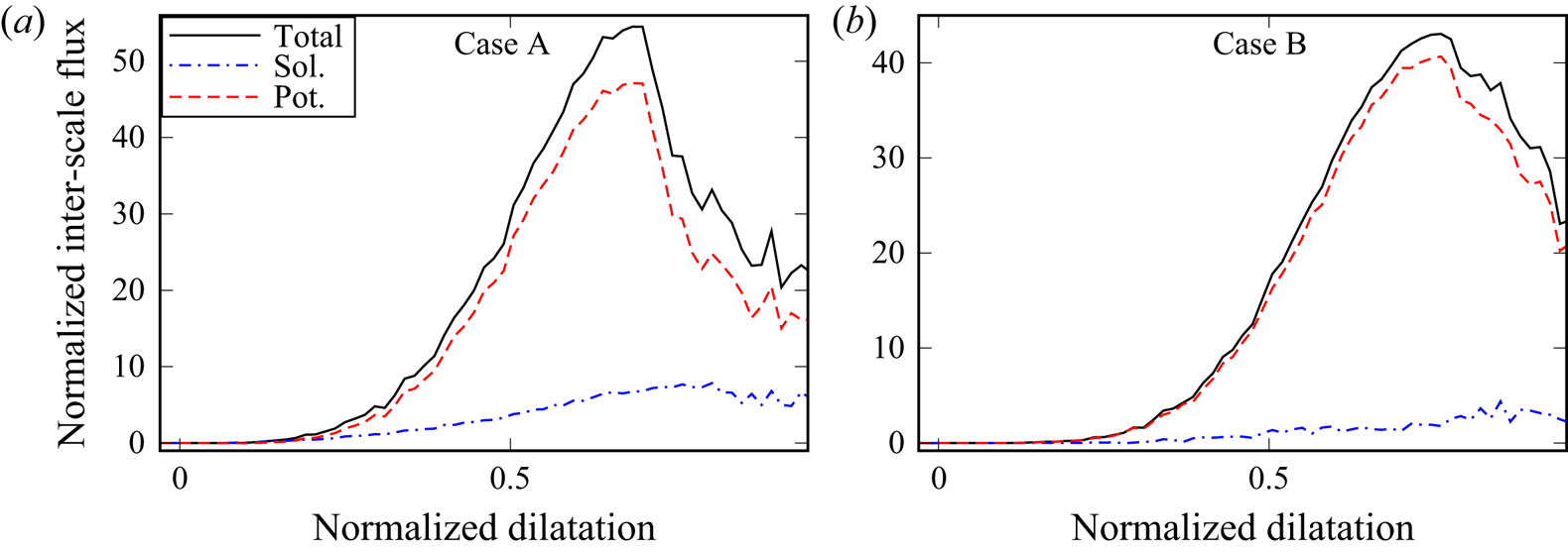
Figure 2. Normalized inter-scale flux  $\delta _L \bar {\rho } \tilde {\boldsymbol {f}} \boldsymbol {\cdot }\boldsymbol {\nabla } \tilde {c}/(\rho _u S_L)$ (black solid lines), as well as solenoidal (
 $\delta _L \bar {\rho } \tilde {\boldsymbol {f}}_s \boldsymbol {\cdot }\boldsymbol {\nabla } \tilde {c}/(\rho _u S_L)$, blue dotted-dashed lines) and potential (
 $\delta _L \bar {\rho } \tilde {\boldsymbol {f}}_p \boldsymbol {\cdot }\boldsymbol {\nabla } \tilde {c}/(\rho _u S_L)$, red dashed lines) contributions to it, conditioned to normalized filtered dilatation
  $\varTheta$ in flames (a) A and (b) B.
  $\varDelta =0.87 \delta _L$.
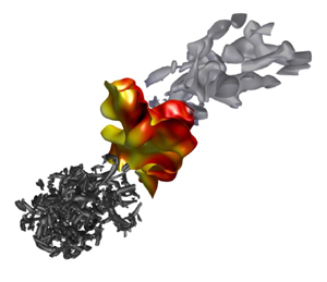
Results plotted in figures 1 and 2 suggest the following physical scenario. Combustion-induced heat release and density drop in instantaneous flames cause the local positive dilatation, thus, injecting kinetic energy into turbulent flow, with the injected energy fluctuating in space and time due to fluctuations in the flame orientation (the local flow accelerates along the normal to the flame). Since solenoidal velocity field is divergence-free, the dilatation causes potential velocity fluctuations. Even if the injection-zone volume (i.e. volume occupied by the flames) is significantly less than the mean flame brush volume, the injected kinetic energy can be statistically significant (Sabelnikov et al. Reference Sabelnikov, Lipatnikov, Nikitin, Hernández-Pérez and Im2022a,Reference Sabelnikov, Lipatnikov, Nikitin, Hernández-Pérez and Imb) due to high local energy-injection rates controlled by the local dilatation. Moreover, the scalar  $c$ is injected into the scalar field within such flames due to the local formation of combustion products. Thus, extra turbulent energy (potential) and extra scalar energy
  $c^2$ are injected at small scales of the order of
  $\delta _L$, with these injections inverting cascade for the scalar
  $c$. Indeed, since the local potential flow accelerates from unburned (
 $c=0$) to burned (
 $c=1$) flame edges, correlation between the local potential velocity and
  $c$ is positive (in the coordinate framework adopted here) within flames and the potential flux
  $\tilde {\boldsymbol {f}}_p$ is predominantly positive (i.e. counter-gradient), thus, making the potential inter-scale flux
  $G_p$ predominantly negative (if the filter contains a flame zone inside it). Appearance of the counter-gradient potential scalar flux
  $\tilde {\boldsymbol {f}}_p$ is confirmed in figure 3 (red dashed lines).
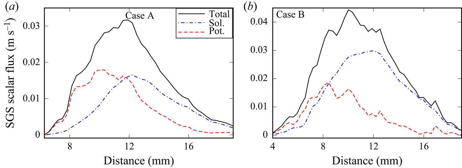
Figure 3. Spatial variations of time- and transverse-averaged axial SGS scalar flux  $\langle\, \tilde {f}_x \rangle$ (black solid lines), as well as solenoidal (
 $\langle\, \tilde {f}_{x,s} \rangle$, blue dotted-dashed lines) and potential (
 $\langle\, \tilde {f}_{x,p} \rangle$, red dashed lines) contributions to it obtained from flames (a) A and (b) B and filtered using a box with sides equal to
  $\varDelta =0.87 \delta _L$.
Comparison of figures 1 and 3 shows two interesting features. First, in the latter figure, magnitudes of  $\langle\, \tilde {f}_{x,s} \rangle$ and
  $\langle\, \tilde {f}_{x,p} \rangle$ are comparable in flame A and the solenoidal flux
  $\langle\, \tilde {f}_{x,s} \rangle$ is even larger than the potential
  $\langle\, \tilde {f}_{x,p} \rangle$ in flame B, whereas
  $|\langle G_p \rangle | \gg |\langle G_s \rangle |$ in both flames (figure 1). This difference between contributions of potential flow to scalar and inter-scale fluxes stems from the fact that the vector
  $\tilde {\boldsymbol {f}}_p$ (
 $\tilde {\boldsymbol {f}}_s$) is more (less) collinear with
  $\boldsymbol {\nabla } \tilde {c}$ (figure 4). The preferential alignment of
  $\tilde {\boldsymbol {f}}_p$ and
  $\boldsymbol {\nabla } \tilde {c}$ is associated with the facts that (i) dilatation and potential velocity are directly linked, whereas
  $\boldsymbol {\nabla }\boldsymbol {\cdot } \boldsymbol {u}_s=0$, and (ii) dilatation in a local flame stems from velocity variations along the local normal to the flame, i.e. along the direction of the vector
  $\boldsymbol {\nabla } c$. The highlighted link of dilatation with the local alignment of the vectors
  $\tilde {\boldsymbol {f}}_p$ and
  $\boldsymbol {\nabla } \tilde {c}$ is further supported in figure 5, which shows that the two vectors are almost collinear if
  $\varTheta = \delta _L \boldsymbol {\nabla }\boldsymbol {\cdot } \boldsymbol {u}/(\tau S_L) > 0.5$ (note that the figure shows
  $- \tilde {\boldsymbol {f}}_p$). This trend is more pronounced in case A characterized by a lower
  $u'/S_L$ and a higher
  $Da$.
$Da$.
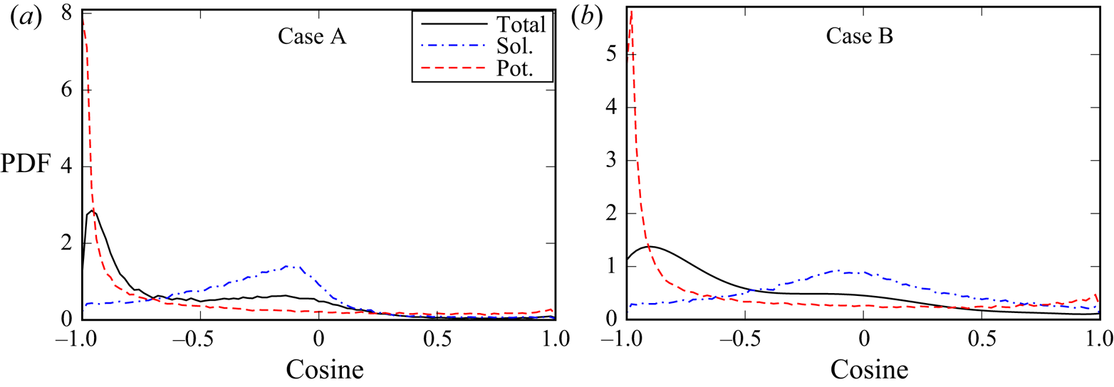
Figure 4. Probability density functions for cosine between vectors  $\tilde {\boldsymbol {f}}$ and
  $\boldsymbol {\nabla } \tilde {c}$ sampled from volumes where
  $0.05 \le \tilde {c}(\boldsymbol {x},t) \le 0.95$ in flames (a) A and (b) B.
  $\varDelta =0.87 \delta _L$. Legends are explained in the caption of figure 3.
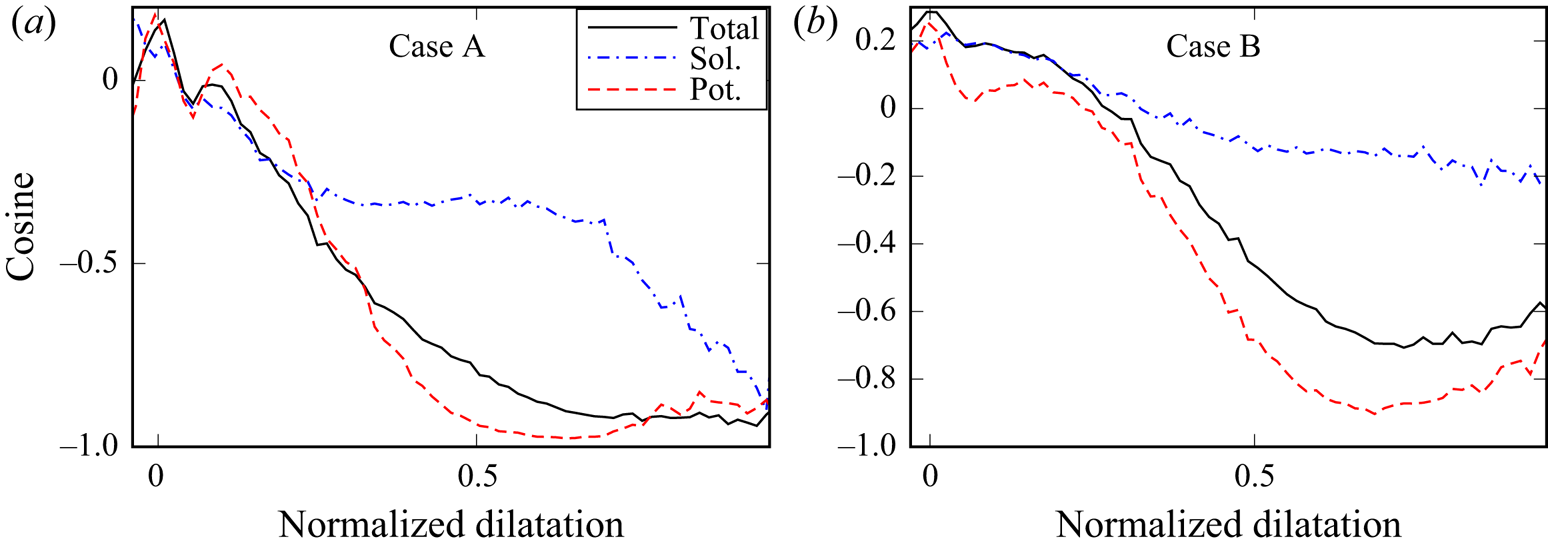
Figure 5. Cosine between vectors  $-\tilde {\boldsymbol {f}}$ and
  $\boldsymbol {\nabla } \tilde {c}$ conditioned to normalized filtered dilatation
  $\varTheta$ in flames (a) A and (b) B.
  $\varDelta =0.87 \delta _L$. Legends are explained in the caption of figure 3.
Second, even the solenoidal scalar flux  $\tilde {\boldsymbol {f}}_s$ shows the counter-gradient behaviour under conditions of the present study (blue dotted-dashed lines in figure 3), thus, making the solenoidal inter-scale flux
  $G_s$ predominantly negative also. However, this phenomenon contributes little to total backscatter (
 $|\langle G_p \rangle | \gg |\langle G_s \rangle |$ in figure 1 due to poor alignment of the vectors
  $\tilde {\boldsymbol {f}}_s$ and
  $\boldsymbol {\nabla } \tilde {c}$ (blue dotted-dashed lines in figures 4 and 5)). Due to a minor contribution of this phenomenon to scalar backscatter, the counter-gradient behaviour of the solenoidal scalar flux is beyond the scope of the present communication. Briefly speaking, the phenomenon results from the smoothing of the flame surface by vorticity generated by baroclinic torque within flames. The reader interested in a more detail discussion is referred to recent studies of a similar phenomenon within RANS framework (Lipatnikov et al. Reference Lipatnikov, Sabelnikov, Nishiki and Hasegawa2018, Reference Lipatnikov, Sabelnikov, Nishiki and Hasegawa2019; Sabelnikov et al. Reference Sabelnikov, Lipatnikov, Nikitin, Nishiki and Hasegawa2021b, Reference Sabelnikov, Lipatnikov, Nikitin, Hernández-Pérez and Im2022b).
5. Concluding remarks
By analysing complex-chemistry DNS data obtained earlier from lean hydrogen–air flames, backscatter of SGS scalar variance is documented not only in weakly turbulent flame A, but also in flame B associated with moderately intense small-scale turbulence and characterized by a unity-order Damköhler number and a ratio of Kolmogorov length scale to thermal laminar flame thickness as low as 0.05.
Application of HHD to the velocity fields yielded by the DNS, followed by an analysis of the obtained solenoidal and potential velocity fields, have shown that the documented backscatter stems primarily from the potential velocity perturbations generated due to dilatation in instantaneous local flames. The backscatter is substantially promoted by a close alignment of the spatial gradient of filtered scalar  $\tilde {c}$ and the potential-velocity contribution to the local SGS scalar flux. The alignment is associated with the fact that combustion-induced thermal expansion increases local velocity in the direction of
  $\boldsymbol {\nabla } c$.
Decomposition of a velocity field into potential (dilatational) and solenoidal (rotational) components is an essential step towards exploring the influence of combustion on cascades of turbulent kinetic energy and mixture non-uniformities.
The above findings call for further development of SGS models of the inter-scale flux  $\bar {\rho } \tilde {\boldsymbol {f}} \boldsymbol {\cdot } \boldsymbol {\nabla } \tilde {c}$ of scalar variance for LES of premixed turbulent combustion.
Acknowledgements
Computational resources for the DNS were provided by the KAUST Supercomputing Laboratory. Valuable comments by the referees are gratefully acknowledged.
Funding
V.A.S. gratefully acknowledges the financial support by ONERA and by the Grant of the Ministry of Science and Higher Education of the Russian Federation (Grant agreement of December 8, 2020 No. 075-11-2020-023) within the program for the creation and development of the World-Class Research Center ‘Supersonic’ for 2020–2025. A.N.L. gratefully acknowledges the financial support by Chalmers Area of Advance Transport. F.E.H.P. and H.G.I. were sponsored by King Abdullah University of Science and Technology (KAUST).
Declaration of interests
The authors report no conflict of interest.


 Open access