


1. Introduction
The meridional overturning circulation is critical in the regulation of the Earth's climate, and understanding the processes essential for maintaining this circulation is of key importance in global climate models. Munk (Reference Munk1966) was amongst the first to suggest that internal gravity waves play a significant part in the deep-water vertical mixing of the density stratification within the open ocean and, hence, the maintenance of these currents. It is now well established that the breaking of internal waves contributes to turbulent mixing in the ocean (Staquet & Sommeria Reference Staquet and Sommeria2002; Wunsch & Ferrari Reference Wunsch and Ferrari2004), yet only recently have the pathways by which internal waves transfer energy to smaller scales and the eventual breaking events been examined in more detail. As noted by Dauxois et al. (Reference Dauxois, Joubaud, Odier and Venaille2018), our understanding of these dissipative mechanisms, as opposed to internal wave generation, leaves several open questions.
Various key mechanisms have been cited for how large-scale internal waves cascade energy to smaller scales. These include internal wave reflection off sloping boundaries (Nash et al. Reference Nash, Kunze, Toole and Schmitt2004), critical angle reflection (Dauxois & Young Reference Dauxois and Young1999) and scattering due to small-scale topography (Peacock et al. Reference Peacock, Mercier, Didelle, Viboud and Dauxois2009). A review by Sarkar & Scotti (Reference Sarkar and Scotti2017) suggests that no single mechanism is responsible for the internal wave contribution to the energy cascade, rather it is a combination of multiple linear and eventually nonlinear processes. MacKinnon & Winters (Reference MacKinnon and Winters2005) and Alford et al. (Reference Alford, MacKinnon, Zhao, Pinkel, Klymak and Peacock2007) suggested that (and subsequently showed Mackinnon et al. Reference Mackinnon, Alford, Sun, Pinkel, Zhao and Klymak2013) equatorward of a critical latitude, (Richet, Chomaz & Muller Reference Richet, Chomaz and Muller2018) parametric subharmonic instability (PSI) plays an important role in the energy transformation of the internal tide into higher-mode near-inertial waves. PSI (which can be viewed a special case of triadic resonance instability (TRI)) is a weakly nonlinear, slowly growing resonant mechanism through which a primary wave is unstable due to infinitesimal perturbations within the flow. As the instability grows, a resonant triad interaction forms whereby the primary wave transfers energy to two secondary waves of lower frequency and shorter length scale (Staquet & Sommeria Reference Staquet and Sommeria2002; Dauxois et al. Reference Dauxois, Joubaud, Odier and Venaille2018). Indeed, Sutherland (Reference Sutherland2013) argues that away from sea-floor boundaries, and neglecting the distorting influence of ocean currents, PSI maybe one of the primary mechanisms for the energy cascade in the abyssal ocean.
In the inviscid limit and under the assumption of an infinite plane wave, the frequencies of the linearly most unstable secondary waves in the triad are equal to half of the primary wave, motivating the traditional terminology of PSI (Fan & Akylas Reference Fan and Akylas2019). Although one often makes the appropriate assumption of oceanic scales being inviscid, in the laboratory setting (where scales are smaller), viscous effects cannot be neglected and resonant wave frequencies deviate away from this subharmonic relationship. Moreover, for certain beam widths, the finite-amplitude manifestation of this instability is unable to access these subharmonic frequencies (Bourget et al. Reference Bourget, Scolan, Dauxois, Le Bars, Odier and Joubaud2014). In the context of a viscous finite-width beam it is therefore more appropriate to consider the mechanism as the more general TRI as opposed to PSI.
The first reported experimental evidence of TRI for internal and interfacial waves was over 50 years ago by Davis & Acrivos (Reference Davis and Acrivos1967), McEwan (Reference McEwan1971) and McEwan & Plumb (Reference McEwan and Plumb1977), who showed that for finite-width beams there exists an amplitude threshold that must be surpassed for instability to occur. This threshold is not found theoretically in the limiting case of an infinite plane wave, where infinitesimal perturbations may induce the development of the instability (Koudella & Staquet Reference Koudella and Staquet2006). In fact, in the special case of a linearly stratified Boussinesq fluid, a plane waveform holds the peculiar property of being an exact solution to the full nonlinear equations at any amplitude (e.g. Thorpe Reference Thorpe1968; Thorpe & Haines Reference Thorpe and Haines1986; Sutherland Reference Sutherland2006), albeit not a linearly stable one. However, although single monochromatic plane waves are convenient mathematically, waves will never take this form in nature. Realistically, oceanic waves are generated from baroclinic tides across ocean ridges and will manifest as beams confined locally in space and therefore broadly distributed over the wavenumber spectrum (Lamb Reference Lamb2004; Gostiaux et al. Reference Gostiaux, Didelle, Mercier and Dauxois2007). The focus of analyses using plane-wave solutions has been highlighted in the review by Dauxois et al. (Reference Dauxois, Joubaud, Odier and Venaille2018), who argue (correctly in our view) that the effects of finite width and envelope shape play an important, but generally overlooked role, when considering the nonlinearities of internal waves.
In attempting to address these concerns, researchers have turned towards exploring the dynamics of TRI in spatially localised internal wave beams. Building on the work of Bourget et al. (Reference Bourget, Dauxois, Joubaud and Odier2013), Bourget et al. (Reference Bourget, Scolan, Dauxois, Le Bars, Odier and Joubaud2014) calculate a growth rate for the instability based on a energy balance that accounts for the role of a finite-width beam. Using direct numerical simulations they also show that the amplitude threshold for instability decreases as the beam width is increased. This decrease is due to any perturbations having a larger spatial field (and hence a longer time) in which to interact with, and extract energy from, the underlying primary beam. These findings align with the theoretical work of Karimi & Akylas (Reference Karimi and Akylas2014), who show how the form of the carrier envelope for a finite-width wave beam has a significant influence on its ability to become unstable based on the wavenumber spectrum produced from the windowing. These works highlight the duality of interpretation for finite-width beams in terms of both the physical parameters and the spectrum in Fourier space.
Triadic resonance can arise due to the sustained spatiotemporal interactions that occur when
 \begin{equation} {\phi_0} = {\phi_1} + {\phi_2}, \end{equation}
where the wave phase,  $\phi _p$, is defined as
 \begin{equation} \phi_p = \boldsymbol{k}_p \boldsymbol{\cdot} \boldsymbol{x} - \omega_p t. \end{equation}
The subscript  $p = (0, 1, 2)$ is used throughout this article to define the primary wave and the two secondary waves, respectively. Both (1.1) and (1.2) are true for three dimensions, but, without loss of generality we can rotate to a two-dimensional (2-D) coordinate system. The 2-D wave vector of wave
  $p$ is defined as
  $\boldsymbol {k}_p = (l_p,m_p)$ with magnitude
  $|\boldsymbol {k}_p| = \kappa _p$, where the components are given in Cartesian coordinates
  $(x,z)$, marked in figure 1, and
  $\omega _p$ denotes the frequency of the wave. In order to distinguish between the three wave beams in the triad and their corresponding parameters, we define
 \begin{equation} \mathbb{B}_p = \{ \rho_p, \varPsi_p; \omega_p, \boldsymbol{k}_p, \varLambda_p \ldots\}, \end{equation}
where  $\mathbb {B}_p$ indicates a wave beam with density perturbation
  $\rho _p$ and stream function
  $\varPsi _p$ fields, frequency
  $\omega _p$, characteristic wavenumber vector
  $\boldsymbol {k}_p$ and beam width
  $\varLambda _p$. In our experiments,
  $\omega _0$,
  $\boldsymbol {k}_0$ and
  $\varLambda _0$ for the primary beam are imposed control parameters, whereas for the secondary beams they arise from the triadic conditions and (weakly) nonlinear dynamics. All triadic wave beams must also satisfy the dispersion relationship for internal waves given as
 \begin{equation} \frac{\omega_p}{N} ={\pm} \cos{\theta_p} ={\pm}\frac{|l_p|}{\sqrt{{l_p}^2 + {m_p}^2}}, \end{equation}
where  $\theta _p$ is the angle between the lines of constant phase and the vertical and
  $l_p$ and
  $m_p$ are the characteristic wavenumber contributions from each beam. Here
  $N$ is the buoyancy frequency of the stratification given by
 \begin{equation} N = \sqrt{-\frac{g}{ \varrho_0}\frac{\partial \bar{\rho}}{\partial z}}, \end{equation}
where  $g$ is the gravitational constant of acceleration. Under the assumptions of a Boussinesq, incompressible fluid, we decompose the total density
  $\varrho$ as
  $\varrho = \varrho _0 + \bar {\rho }(z) + \rho (x,z,t)$, where
  $\varrho _0$ is the reference density,
  $\bar \rho$ is the background density stratification as a function of depth and
  $\rho$ is the perturbation density. We consider the density changes from perturbations and background stratification to be small compared to the reference density, so that
  $\bar \rho$,
  $\rho \ll \varrho _0$.

Figure 1. (a) A schematic showing the front view of the tank as would be seen by the camera. The wavemaker is located along a 1 m section of the tank floor, 2.5 m and 7.5 m away from the left and right boundary wall, respectively. The tank is filled with a 0.45 m salt stratification. A conductivity probe, mounted above the tank, measures the density profile. (b) A schematic showing the side view of the tank in order to visualise the optical arrangement for synthetic schlieren. The thermal tunnel is not shown for clarity.
Given the triadic resonant condition in (1.1), it is easy to assume that the instability selects one particular triad, composed of three distinct frequencies and wavenumbers for all time. More recently, our understanding of triad selection is evolving for finite-width beams. Indeed, while examining the transient start up of the instability, Koudella & Staquet (Reference Koudella and Staquet2006) noted that not just one triad is responsible for the initial instability, rather, a number of triads form around the maximum linear growth rate. This is further developed by Ghaemsaidi & Mathur (Reference Ghaemsaidi and Mathur2019) who showed how the width of the peak of the growth rate curves broadens with increased amplitude. In addition, recent work by Fan & Akylas (Reference Fan and Akylas2020) showed how classic TRI theory is unable to explain the instability in the context of a thin beam due to the broadband wavenumber spectrum corresponding to the primary beam.
The novelty of the present paper lies in the examination of the long-term evolution of the instability. This is of key importance when we consider internal tides. As noted by Karimi & Akylas (Reference Karimi and Akylas2017), time harmonic internal wave of locally confined profile (such as those considered this work) naturally arise from the interaction of barotropic flow over topography. Owing to the 11-m-long tank used in the experimental set-up, we are able to observe the experiment for hours without interference from side wall reflections or significant changes to the stratification. We show experimentally that, over long time scales, the constituent triadic waves synchronously modulate in amplitude and in the physical location of the two secondary wave beams. Further investigation shows that part of these modulations are coincident with the growth and decay of separate triads, all linked through the primary wave beam. Through 2-D weakly nonlinear modelling, we are then able to show how the evolution of the instability in a finite-width beam is remarkably sensitive to these separate triads. This sensitivity is due to their affect on the residence time of the secondary wave beams with the underlying primary beam.
The outline of the remainder of this article is as follows. In § 2 we detail the experimental set-up and processing procedure. In § 3 we then present the experimental results, looking first at the initial observations in § 3.1 and then at the long-term evolution of the experiments in § 3.2. Based on these observations, we present the perturbation expansion that forms the basis of the 2-D weakly nonlinear model in § 4. In § 5 we present the results of the model. We start with § 5.1, where we examine the weakly nonlinear interactions on their own before moving onto § 5.2, where the results of the weakly nonlinear 2-D model are given. Conclusions are then drawn in § 6.
2. Experimental procedure
2.1. Experimental set-up
Experiments were undertaken in an 11-m-wide, 0.48-m-deep, 0.29-m-wide Perspex (acrylic) tank. Along a 1 m section of the tank floor, 2.5 m from the left-hand wall of the tank, sits the Arbitrary Spectrum Wave Maker (ASWaM), also known as the ‘magic carpet’. This flexible horizontal boundary can generate sinusoidal forcing (Beckebanze et al. Reference Beckebanze, Grayson, Maas and Dalziel2021; Dobra, Lawrie & Dalziel Reference Dobra, Lawrie and Dalziel2021, Reference Dobra, Lawrie and Dalziel2022) (as well as aperiodic configurations (Dobra, Lawrie & Dalziel Reference Dobra, Lawrie and Dalziel2019)), with the ability to vary amplitude, frequency and wavenumber in both the temporal and spatial domains. The wavemaker is composed of a series of 96 computer-controlled linear actuators that sit below the tank. Each actuator is mounted to a vertical drive rod that passes through the base of the tank and connects to a 0.28-m-long horizontal rod that spans the tank width. These rods are spaced at 10 mm intervals along the wavemaker. A 3-mm-thick neoprene foam sheet covers the full length and width of the wavemaker, thus interpolating between the horizontal rods to allow smooth forcing. The lengthwise edges of the neoprene slide against the tank walls. Provided the chosen waveforms preserve a zero-mean displacement across the length of the flexible surface, the pressure gradient available to drive flow around the edges of the neoprene foam is negligible. Thus, flow in either direction between the cavity and the visualisation region may be considered negligible. A 80 mm layer of glycerol is added to the 80-mm-deep cavity below the neoprene to largely eliminate salt water from around the seals through which the drive rods pass. The glycerol thus helps prevent leakage past the seals due to salt crystallising within them. When submerged in a stratified fluid, the wavemaker can generate quasi-2-D, internal wave beams at amplitudes sufficient to permit wave breaking at distances away from the source. For full details of ASWaM's construction, see Dobra (Reference Dobra2018) and Dobra et al. (Reference Dobra, Lawrie and Dalziel2019).
The procedure for filling the tank is as follows. First, the glycerol is gravity fed into the wavemaker cavity. The tank is then filled over the course of 8 h with a linear salt stratification using two computer-controlled gear pumps, (Coleparmer Ismatec BVP-Z Analog gear pump drives fitted with Micropump L20562 A-Mount Suction Shoe pump heads) controlled via the software DigiFlow (Dalziel et al. Reference Dalziel, Carr, Sveen and Davies2007). Each pump draws from either a fully saturated salt water or fresh water reservoir. This filling method allows for more precise control of the density stratification compared with the traditional double bucket technique (Oster & Yamamoto Reference Oster and Yamamoto1963), enabling the density gradient and fluid depth to be pre-determined. The depth of the stratification is  $H = 0.45 \pm 0.01$ m.
To measure the density profile created by the pumps, an aspirating conductivity probe is mounted to a linear traverse above the tank. One minute before the start and one minute after the end of an experiment, the probe is traversed downwards through the stratification to measure the conductivity of the saline solution passing through the probe tip. For the experimental campaign reported here, a linear density stratification with a buoyancy frequency  $N = 1.54$ rad s
 $^{-1}$ is used. As the week progresses, a mixed layer develops at the free surface and at the bottom of the tank. This layer acts to reduce transmission from the wavemaker but does not change the density gradient in the middle of the tank. A schematic of the tank, as viewed from the front, can be seen in figure 1(a).
2.2. Wave visualisation
Synthetic schlieren (Dalziel, Hughes & Sutherland Reference Dalziel, Hughes and Sutherland2000; Dalziel et al. Reference Dalziel, Carr, Sveen and Davies2007) is used to visualise our experiments. This non-intrusive technique takes advantage of the differential refraction of light in a refractive index gradient and the Gladstone–Dale relationship between refractive index and fluid density, such that light rays curve towards regions of higher density. Internal waves cause local perturbations to the density field and, thus, the direction of light rays passing through them will also be perturbed. The resulting distortion of a textured background image yields a measurable signal associated with the density perturbations. To minimise the effects of convective thermal fluctuations on the synthetic schlieren measurements in the air between the tank and the camera, a ‘thermal tunnel’ spans from the camera lens to the perimeter of the visualisation region on the tank.
A random dot pattern attached to an LED light bank is located  $0.20 \pm 0.04$ m behind the tank and a 12-megapixel ISVI IC-X12CXP camera with a Nikkor 35–135 mm zoom lens is located
  $3.50 \pm 0.10$ m from the front. This optical arrangement is shown in the side-view schematic in figure 1(b). The large distance between the camera and the tank was chosen in order to reduce parallax (Thomas, Marino & Dalziel Reference Thomas, Marino and Dalziel2009).
We compute the line-of-sight mean of the gradient vector of the density perturbation field  $\rho$, which for convenience we non-dimensionalise according to
 \begin{equation} {\boldsymbol{\beta} = (\beta_x, \beta_z) = \frac{g}{N^2\varrho_0}\left(\frac{\partial{\rho}}{\partial x}, \frac{\partial{\rho}}{\partial z}\right)}. \end{equation}
Our experiment is configured to generate and diagnose quasi-2-D internal wave structures, up to the limit of wave breaking, the point at which the mapping of ray paths to density perturbations is no longer an aim.
2.3. Internal wave forcing
The experimental campaign presented in this article is composed of 36 experiments. To reduce uncertainties associated with the test conditions both within the tank and in the laboratory ambient, the campaign was run within a 7 day period without refilling the tank, allowing a period of 3 hours between each experiment for any residual motion to dissipate.
Following arguments laid out by Dobra et al. (Reference Dobra, Lawrie and Dalziel2019), for all the experiments in this campaign the vertical displacement  $z = h(x,t)$ imposed on the neoprene foam to generate the primary beam,
  $\mathbb {B}_0$, is
 \begin{equation} z = h(x,t) =
\begin{cases} \displaystyle \text{Re}\left(f(t) \, {\rm e}^{{\rm
i} l_0 x} \cos^2\left(\frac{x-B}{8{\rm \pi}^2}\right)\right), &
A < x < B,\\ \text{Re}(f(t) \, {\rm e}^{{\rm
i} l_0 x} ), & B < x < C, \\
\displaystyle \text{Re}\left(f(t) \, {\rm e}^{{\rm i} l_0 x}
\cos^2\left(\frac{x-C}{8{\rm \pi}^2}\right)\right), & C < x < D,
\\ 0, & \text{otherwise}, \\
\end{cases} \end{equation}
\begin{equation} z = h(x,t) =
\begin{cases} \displaystyle \text{Re}\left(f(t) \, {\rm e}^{{\rm
i} l_0 x} \cos^2\left(\frac{x-B}{8{\rm \pi}^2}\right)\right), &
A < x < B,\\ \text{Re}(f(t) \, {\rm e}^{{\rm
i} l_0 x} ), & B < x < C, \\
\displaystyle \text{Re}\left(f(t) \, {\rm e}^{{\rm i} l_0 x}
\cos^2\left(\frac{x-C}{8{\rm \pi}^2}\right)\right), & C < x < D,
\\ 0, & \text{otherwise}, \\
\end{cases} \end{equation}
where the locations  $A$,
$A$,  $B$,
$B$,  $C$ and
  $D$ are
  $7{\rm \pi} /|l_0|$,
  $9{\rm \pi} /|l_0|$,
  $13{\rm \pi} /|l_0|$ and
  $15{\rm \pi} /|l_0|$, respectively, and
  $l_0$ is the horizontal component of the primary wave vector
  $\boldsymbol {k}_0 = (l_0, m_0) = (-0.05, -0.06)$ mm
 $^{-1}$. This gives a horizontal wavelength for the primary beam of
  $\lambda _{x_0} = 2{\rm \pi} /|l_0| = 125.66$ mm.
As we restrict  $\omega _p > 0$ (for all
  $p$, where
  $p = (0, 1, 2)$ for the primary and two secondary beams, respectively); having
  $l_0, m_0 < 0$ means the group velocity of the primary wave beam is initially propagating upwards and to the left. The spatial structure of the forcing, described by (2.2), takes the form of a beam with the inner two wavelengths reaching maximum amplitude and the outer wavelengths being smoothed by a cosine-squared envelope. Due to this cosine squared smoothing on the edges of the beam profile, we do not consider the width,
  $D - A$, for energy transfer. Rather, we estimate the contribution from one of the smoothed edges using the integral measure employed by Dalziel, Linden & Youngs (Reference Dalziel, Linden and Youngs1999), giving a horizontal beam width of
 \begin{equation} \varLambda_{x_0} = \varLambda_{0} / \cos\theta = 2\lambda_{x_0} + 2\int_{0}^{\lambda_{x_0}} \alpha (1 - \alpha) {{\rm d}\kern0.7pt x} = 277.41\ \textrm{mm}, \end{equation}
where  $\varLambda _{0}$ is the full beam width and
  $\alpha = \cos ^2(x/8{\rm \pi} ^2)$ is the smoothing function on the outer flanks of the beam profile. The temporal forcing
  $f(t)$ is then described as
 \begin{equation} f(t) = \begin{cases} 0, & t \leq 0\ \mathrm{s}, \\ \displaystyle {A_0} \left(\frac{t}{30}\right)\,{\rm e}^{-{\rm i} \omega_0 t}, & 0 \leq t \leq 30 \ \mathrm{s}, \\ {A_0} \hspace{0.6mm}\,{\rm e}^{-{\rm i}\omega_0 t}, & 30 \ \mathrm{s} \leq t \leq t_{end} -30 \ \mathrm{s} , \\ \displaystyle {A_0} \hspace{0.6mm}\left(\frac{t_{end} -t}{30}\right) \,{\rm e}^{-{\rm i}\omega_0 t}, & t_{end} -30 \ \mathrm{s} \leq t \leq t_{end} , \end{cases} \end{equation}
where  $\omega _0$,
  ${A_0}$ and
  $t_{end}$ are respectively, the forcing frequency of 0.95 rad s
 $^{-1}$, the nominal forcing amplitude in millimetres of the primary beam and the end time of the experiment in seconds. Experiments are captured at 1 frame per second (f.p.s.), which is more than sufficient to capture the fast time evolution of the wave field given by the primary beam period
  $T_0 = 2{\rm \pi} / \omega _0$.
The only two parameters to be varied in this experimental study are  $t_{end}$ and
  ${A_0}$. The run time,
  $t_{end}$, is either 90 or 180 min, while the non-dimensional amplitude
  ${|l_0|A_0}$ ranges between 0.175–0.225. The input amplitude threshold for the instability is achieved at
  ${|l_0|A_0} \approx 0.194$, increasing by
  $0.013$ throughout the week due to the slow growth of a mixed layer along the bottom of the tank which reduces wave transmission (see Sutherland & Yewchuk (Reference Sutherland and Yewchuk2004) for a discussion on the transmission). Our focus is on the weakly nonlinear regime, so we seek to minimise unnecessary mixing induced by wave actuation and limit our amplitudes to those just sufficient to exceed the instability threshold calculated by Davis & Acrivos (Reference Davis and Acrivos1967).We do not force any wave amplitudes large enough to permit wave breaking.
As the tank extends well beyond the field of view in both directions, internal wave beams with typical dominant wavenumbers of  $\boldsymbol {k}_0 = (-0.05, -0.06)$ mm
 $^{-1}$ reflecting off the far left-hand wall of the tank return to the viewing region with only 2
  $\%$ of their original amplitude, due to viscous dissipation over an approximately 5 m horizontal travel distance. We thus consider wave–wave interactions involving these reflected beams to be negligible. We also highlight that several similar sets of experiments (not presented here) were conducted but with a rightward propagating primary beam, resulting in approximately 15 m of horizontal travel before re-interaction. These experiments exhibited the same behaviour as those presented in this article using a leftward propagating beam.
3. Experimental results
3.1. Initial observation and analysis
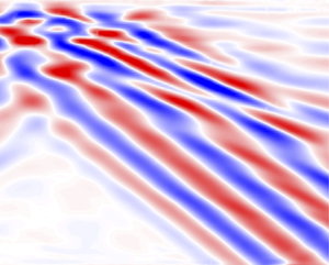
We start by examining one experiment from the set of 36 with an imposed amplitude displacement of  ${|l_0|A_0} = 0.200$. Figure 2(a) shows
  $\beta _z$ over the visualisation region at
  $t/T_0 = 83$. Here,
  $\mathbb {B}_0$, representing the primary wave beam generated by the wavemaker, propagates energy up and to the left, at its respective group velocity
  $\boldsymbol {c}_{g_0}$. The group velocity is defined for all wave beams by
 \begin{equation} \boldsymbol{c}_{g_p} = \left(\frac{\partial}{\partial l_p}, \frac{\partial}{\partial m_p} \right) \omega_p = \frac{N l_p}{\kappa_p^3} (m_p, -l_p), \end{equation}
where the broadband wavenumber spectrum of each beam is approximated with a characteristic wavenumber. The primary beam  $\mathbb {B}_0$ reflects off the free surface, causing
  $\theta$, and hence the vertical component of its group velocity, to change sign and the wave packets subsequently move down and to the left. An appropriate Reynolds number for the flow is given by
  $Re = |\boldsymbol {c}_{g_0}|/(\nu \kappa _0) = N\sin \theta / (\nu \kappa _0^2$), where
  $\nu = \mu /\varrho _0$ is the kinematic viscosity of 1 mm
 $^2$ s
 $^{-1}$. Here,
  $|\boldsymbol {c}_{g_0}|$ provides the velocity scale and
  $\kappa _0$ provides the length scale. As described by Hazewinkel (Reference Hazewinkel2010), this definition of Reynolds number is chosen as wave amplitude decays exponentially in the direction of
  $\boldsymbol {c}_{g_0}$. Using this definition,
  $Re \approx 170$. As the selected input amplitude displacement of
  ${|l_0|A_0} = 0.200$ is above the instability threshold,
  $\mathbb {B}_0$ becomes unstable, leading to the formation of two secondary beams. One of these beams,
  $\mathbb {B}_1$, is clearly visible in figure 2(a). This beam emanates from the central region of
  $\mathbb {B}_0$ but moves in nearly the opposite direction, with a group velocity down and to the right. From figure 2(a), the third beam,
  $\mathbb {B}_2$, that completes the triad is not visible. In order to understand the underlying modal structure of these beams, the flow field
  $\boldsymbol {\beta }$, is decomposed using dynamic mode decomposition (DMD).

Figure 2. (a) The non-dimensional vertical gradient of the density perturbation  $\beta _z$ of the flow field at
  $t/T_0 = 83$ into an experiment forced at
  ${|l_0|A_0} = 0.200$. (b)–(d) The real part of
  $\beta _z$ for three of the dominant frequencies produced from the DMD over
 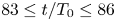 $83 \leq t/T_0 \leq 86$. The black arrows overlaid indicate the orientation of the respective wavenumber vectors
  $\boldsymbol {k}_p$. In panel (b) we see solely the wave field
  $\mathbb {B}_0$ with
  $\omega _0/N = 0.62$. In (c) we see
  $\mathbb {B}_1$ with
  $\omega _1/N = 0.23$ and in (d)
  $\mathbb {B}_2$ with
  $\omega _2/N = 0.39$. The black box in (b) shows the spatial averaging domain
  $\langle \rangle _r$ used for the primary beam, discussed in § 5.1.
DMD works by performing an eigendecomposition of a linearised representation of the underlying evolution operator for a given flow field (Schmid Reference Schmid2010). The ‘dynamic modes’ are the recurrent spatial structures that accurately describe the dominant behaviour captured in the data sequence. Where DMD excels is in determining the frequencies and structure of the modes from short time series where there is a discrete spectrum that can reasonably be approximated by a combination of delta functions at slowly evolving frequencies. The ability to extract the modes from short time series allows exploration of the slowly evolving structure and frequency of the modes. This linear approximation for the evolution operator is valid for the experiments shown here due to the two discrete time scales, whereby the slow time evolution of the beam amplitude is much less than the fast time scales  $\omega _p t$.
The maximum number of dynamic modes is given by the number of input frames in the sequence  $\delta t$ (in this case
  $\delta t = 20$ s, as we use a frame rate of 1 f.p.s., which is just greater than the slowest period of the triad
  $T_1$) and if the obtained mode is complex then it is coupled as a conjugate pair (representing an oscillatory mode). Here, however, we are only interested in those modes with an eigenvalue modulus very close to one, as they represent the steady, non-decaying modes of the system. When instability occurs experimentally, four non-decaying modes are obtained, three of which are conjugate pairs of eigenvalues. The real part of these three modes produced over the temporal window
  $83 \leq t/T_0 \leq 86$ are given in figures 2(b)–2(d). As expected from the input forcing, figure 2(b) corresponds to the input
  $\mathbb {B}_0$ with non-dimensional frequency
  $\omega _0/N= 0.62$. Figure 2(c) then corresponds to
  $\mathbb {B}_1$ with
  $\omega _1/N = 0.23$ and figure 2(d) to
  $\mathbb {B}_2$ (obscured behind
  $\mathbb {B}_0$ in figure 2a), which propagates with a group velocity up and to the left, with non-dimensional frequency
  $\omega _2/N = 0.39$. We sum the frequencies of the secondary beams and see that the temporal condition for triadic resonance,
  $\omega _0 = \omega _1 + \omega _2$, is satisfied. We remark that this frequency relationship is not enforced at any stage of experimental post-processing, but arises naturally from prominent signals found in the temporal spectrum.
The fourth (non-decaying mode) corresponds to  $\omega /N = 0$ and is not shown here. This is generated from a two-wave interaction (TWI), in which two wave beams interact to produce a third wave beam, with a phase angle relationship
 \begin{equation} \check{\phi} ={\pm} \phi_0 \mp \phi'_{0}. \end{equation}
In this case,  $\phi _0 = l_0 x + m_0 z - \omega _0 t$, corresponds to the phase angle of
  $\mathbb {B}_0$, and
  $\phi '_{0} = l_0 x - m_0 z - \omega _0 t$ to its reflection,
  $\mathbb {B}'_{0}$, from the free surface. These wave beams will sum to produce a third wave beam with wavenumber vector
  $\check {\boldsymbol {k}} = (0, 2m_0)$ aligned with the vertical and with zero frequency. This non-propagating disturbance cannot be classed as a wave, but instead should be treated as a forced oscillatory structure that is confined to the interaction region of the primary beam with its reflection. If considered analytically (Thorpe & Haines Reference Thorpe and Haines1986) or numerically (Grisouard et al. Reference Grisouard, Leclair, Gostiaux and Staquet2013) (unfortunately, this manuscript contained a typo in the lead author's name when published and so may appear elsewhere with the lead author (incorrectly) set to ‘Grisouarda’; here we have reverted to the correct spelling of the lead author's name, ‘Grisouard’) in a 2-D setting, only weak horizontal vorticity is generated (with zero Lagrangian mean flow, indicating no mass transport), which is partially suppressed by the background stratification (Beckebanze, Raja & Maas Reference Beckebanze, Raja and Maas2019). When considered in a three-dimensional (3-D) setting, however, Grisouard et al. (Reference Grisouard, Leclair, Gostiaux and Staquet2013) showed, both experimentally and numerically, how a stronger slowly evolving 3-D horizontal mean flow develops from the interaction region of the primary beam with its reflection. This flow has a vertical component to its vorticity field and non-zero Lagrangian mean flow. Indeed, if viscous attenuation and cross-beam variations are present, it is possible for this 3-D Lagrangian mean flow to be generated from the wave beam interacting with itself, as shown analytically by Kataoka & Akylas (Reference Kataoka and Akylas2015) and experimentally by Bordes et al. (Reference Bordes, Venaille, Joubaud, Odier and Dauxois2012). In all of the 3-D cases cited previously, however, the wave beam is propagating in a tank wider than the beam width. This allows for a recirculating mean flow to develop in the transverse direction, outside of the spatial extent of the beam. As noted by Sutherland (Reference Sutherland2006) in experiments where wave beams are confined laterally by tank side walls, as is the case in the experiments presented here, horizontal mean flow of this type is unable to develop. Despite this, the presence of the lateral side walls will act to induce a mean flow in the boundary layer, as discussed by Horne et al. (Reference Horne, Beckebanze, Micard, Odier, Maas and Joubaud2019). They showed how a wavemaker spanning the full width of the tank will directly force a mean flow in the lateral boundary layer, balanced by a return flow in the interior. Due to our large tank dimensions, however, a theoretical steady state would not be achieved until approximately 5 h (with a boundary layer thickness of
  ${\sim}1$ mm) and the return flow would remain weaker than the 2-D dynamics described here. Overall, the observed zero-frequency mode in our experiments, closely resembles the 2-D simulations of Grisouard et al. (Reference Grisouard, Leclair, Gostiaux and Staquet2013) and, although the disturbance does slowly exit the interaction region of
  $\mathbb {B}_0$ and
  $\mathbb {B}'_{0}$, indicating the slow growth of a Lagrangian mean flow, its amplitude remains small and no strong reticulation is seen to develop and as such does not affect the evolution of TRI.
We proceed to determine the wave vectors corresponding to the primary and secondary wave beams by taking our frequency-decomposed gradient field over the temporal window  $83 \leq t/T_0 \leq 86$, the real parts of which are shown in figures 2(b)–2(d), and calculating a 2-D power spectrum on each constituent field separately. Each image is embedded in a zero-filled matrix in order to improve resolution and limit spatial aliasing. The wavenumber is determined by fitting a quadratic curve to the peak of the resultant power spectra and finding the wavenumber corresponding to the peak of the curve. This procedure is performed on every row and column of the domain and subsequently mean averaged over both spatial dimensions. The smallest resolvable length scale is 2 pixels, equivalent to the non-dimensional length
  $x|l_0| = 0.031$, given by the ratio of pixel resolution to region size. As the analysis performed on the horizontal density gradient
  $\beta _x$ provides similar results to that of the vertical
  $\beta _z$, we use only the results from the vertical gradient for simplicity. The non-dimensional characteristic wavenumbers for the vertical gradient fields shown in figure 2 are
  $\boldsymbol {k}_0/|l_0| = (-1.00, -1.32)$,
  $\boldsymbol {k}_1/|l_0| = (0.59, 2.32)$, and
  $\boldsymbol {k}_2/|l_0| = (-1.58, -3.82)$. These wave vectors are shown by the blue arrows on figure 3, where the underlying black, red and green curves provide the locus of all possible solutions for
  $\boldsymbol {k}_1$ given
  $\boldsymbol {k}_0$, based on both the dispersion relationship (1.4) and the TRI condition (1.1).

Figure 3. The underlying solid and dashed black, red and green curves give all of the possible locations for the tip of  $\boldsymbol {k}_1$ that satisfy both the dispersion relationship (1.4) and the TRI condition (1.1) for a given
  $\mathbb {B}_0$. The dark blue arrows show the experimentally produced, characteristic, wavenumber vectors of the resonant triad shown in figure 2, obtained from taking the Fourier transform in
  $(x,z)$ of the gradient field. The shaded grey region then indicates the range of wavenumber vectors obtained over the course of the experiment. The six dark blue marks correspond to the different triad wave vector configurations
  $\mathbb {T}$ used in the weakly nonlinear modelling and are discussed in § 5.1. The panel in the bottom right corner shows an enlarged view of the region enclosed by the black rectangle.
Although the calculated characteristic wave vectors shown in figure 3 form almost in a closed triangle, their alignment is not perfect, potentially indicating that the spatial triadic resonance condition  $\boldsymbol {k}_0 = \boldsymbol {k}_1 + \boldsymbol {k}_2$ is not exactly satisfied. The reason for this slight misalignment is due to three factors. First, there is the effect of inevitable experimental noise. Second, as we are considering finite-width beams as opposed to plane waves, each beam is composed of a broadband wavenumber spectrum. By defining a single characteristic wavenumber for the beam, taken from the peak of the Fourier spectrum, we are therefore approximating this wavenumber distribution. Third, we are assuming that the spatial structures of
  $\mathbb {B}_1$ and
  $\mathbb {B}_2$ are uniform over the field of view. In fact, as the experiment progresses, significant modulations to the structures of
  $\mathbb {B}_1$ and
  $\mathbb {B}_2$ are observed, revealing that this assumption of spatial uniformity is only an approximation.
Although it is clear that TRI was indeed being witnessed experimentally in a finite-width beam, this in itself is not novel. In an experiment actuated by an oscillating cylinder, Clark & Sutherland (Reference Clark and Sutherland2010) attributed the breakdown of a wave beam due to TRI, showing how the instability evolves from infinitesimal perturbations in the flow. This work has recently been developed further by Fan & Akylas (Reference Fan and Akylas2020), who discussed the validity of TRI theory in thin wave beams. Moreover Joubaud et al. (Reference Joubaud, Munroe, Odier and Dauxois2012) and Bourget et al. (Reference Bourget, Dauxois, Joubaud and Odier2013) clearly showed the growth of the instability for a finite-width beam in experiments using their sidewall wavemaker. In our work, the regime of interest is not the initial growth of the instability, but rather the finite-amplitude unsteady modulations that occur afterwards. As noted, the expected saturated equilibrium state for the weakly non-linear instability is not observed, rather we witness slow modulations of the amplitudes and structures of the constituent beams in the triad, revealing much more dynamical behaviour than anticipated. We investigate the long-term evolution of this unsteady behaviour for the remainder of the paper.
3.2. Long-time development
Figure 4 shows 8 instantaneous images of the experiment shown in figure 2. Figure 4(a) (the same image shown in figure 2a) is captured at  $t/T_0 = 83$ into the experiment, just as
  $\mathbb {B}_0$ becomes visibly unstable. By
  $t/T_0 = 180$, shown in 4(b),
  $\mathbb {B}_1$ has clearly developed, with a group velocity propagating down and to the right. A particularly interesting feature of the subsequent time frames is the modulation of
  $\mathbb {B}_1$ over time. Not only is its region of generation not constant, it migrates across the full height of
  $\mathbb {B}_0$, the beam itself also varies in both intensity and width. This migratory behaviour, along with the aperiodic growth and decay persists for the full duration of the experiment, which lasts for over 800 periods of the primary beam. Further quantitative analysis of this peculiar behaviour requires us to calculate the amplitude of the individual resonant wave beams
  $\mathbb {B}_0$,
  $\mathbb {B}_1$ and
  $\mathbb {B}_2$. Decomposing by frequency into complex constituent fields using DMD, we calculate the vertical displacement field by
 \begin{equation} {\xi}_p(x,z) = \int_x \int_z \boldsymbol{\beta} \partial z \partial x = \frac{g}{N^2}\frac{\rho_p}{\varrho_0}, \end{equation}
where  $\rho _p$ is the full density perturbation field found by a least squares minimisation of the integrated horizontal and vertical components of the density gradient (Hazewinkel, Maas & Dalziel Reference Hazewinkel, Maas and Dalziel2011). We assume an oscillatory form
  $\rho _p = \tilde {\rho }_p\, {\rm e}^{{\rm i}\phi _p}$ and
  ${\xi }_p = \tilde {{\xi }}_p\, {\rm e}^{{\rm i}\phi _p}$, where
  $\tilde {\rho }$ and
  $\tilde {{\xi }}$ are the slowly varying complex density and vertical amplitude fields, respectively, varying on a slow time scale well separated from the oscillation period of all wave beams in the system.

Figure 4. Sequence of images showing the non-dimensional vertical gradient of the density perturbation  $\beta _z$, for the same experiment shown in figure 2 with a forcing amplitude of
  ${|l_0|A_0} = 0.200$. The timings of the images are (a)
  $t/T_0 = 83$, (b)
  $t/T_0 = 180$, (c)
  $t/T_0 = 294$, (d)
  $t/T_0 = 347$, (e)
  $t/T_0 = 450$, (f)
  $t/T_0= 481$, (g)
  $t/T_0 = 628$ and (h)
  $t/T_0 = 660$. These timings have been chosen to correspond to interesting features in the constituent vertical amplitude fields of the triad beams and are marked by the black dashed lines on figure 5(a). The black lines in (c) indicate where the
  $\mathbb {B}_1$ beam changes wavenumber, evidenced by the subtle change in wavelength in between the two lines.
We then isolate the wave beam of interest further using a Hilbert transform, first used for internal waves by Mercier, Garnier & Dauxois (Reference Mercier, Garnier and Dauxois2008). This filtering technique is applied to isolate the quadrant of Fourier space containing the wave vectors of the beam of interest from other signals of the same temporal frequency (e.g. separating  $\mathbb {B}_0$ from its reflection from the free surface,
  $\mathbb {B}'_0$). We then take the root mean square (magnitude) of the complex output, leaving the constituent positive scalar fields
  $|\tilde {{\xi }}_p|$, containing only the triadic wave beam,
  $p$, of interest.
In order to have a single value for amplitude that is independent of space, we then spatially mean average  $|\tilde {{\xi }}_p|$ over the whole field of view denoted
  $\langle |\tilde {{\xi }}_p| \rangle _w$. This choice of spatial averaging ensures that our measure of amplitude is decorrelated with the position of a beam in space, a topic that is discussed further in § 5.1. An unavoidable consequence of this choice, however, is that this average measure no longer represents the local amplitude within a beam. To account for this, the other region used for spatial averaging is shown by the black box in figure 2(b), which we denote as
  $\langle |\tilde {{\xi }}_0|\rangle _r$. This region is only ever used for the primary beam and is used to compare the experimental input amplitude with the 0-D modelling discussed in § 5.1.
Figure 5 shows the spatially averaged, non-dimensional vertical amplitude  $|l_0| \langle |\tilde {{\xi }}_p|\rangle _w$ (wave steepness) for two experiments. In figure 5(a) we show the same experiment as figure 4, whereas figure 5(b) corresponds to another experiment with the same forcing amplitude (
 ${|l_0|A_0} = 0.200$) but with a much longer run time (
 $t_{{end}}/T_0 = 1633$). We first note that the growth of the secondary wave beams appears earlier in figure 5(a) than figure 5(b) and that the maximum amplitude of the primary wave beam in figure 5(a) is larger, despite both experiments having the same input amplitude displacement,
  ${|l_0|A_0}$, from the wavemaker. This is due to the growth of a mixed layer at the bottom of the tank, which results in decreased transmission from the wavemaker to
  $\mathbb {B}_0$ as the week progresses. Despite both experiments having the same forcing amplitude, as the experiment in figure 5(b) was conducted 2 days after the experiment in figure 5(a), the resultant amplitude of
  $\mathbb {B}_0$ is less. As noted by Mercier et al. (Reference Mercier, Martinand, Mathur, Gostiaux, Peacock and Dauxois2010), this emphasises the need to use the measured wave beam amplitude as opposed to the imposed displacement from the wavemaker.

Figure 5. The non-dimensional vertical amplitude  $|l_0| \langle |\tilde {{\xi }}_p|\rangle _w$ of
  $\mathbb {B}_0$ (blue),
  $\mathbb {B}_1$ (red),
  $\mathbb {B}_2$ (green) for two experiments. The spatial averaging of each amplitude field is performed over the whole domain
  $\langle \rangle _w$. (a) The same experiment shown in figure 4 with run time of
 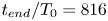 $t_{{end}}/T_0 = 816$ and input amplitude
  ${|l_0|A_0} = 0.200$. The black dashed lines mark the timings of the images in figure 4. (b) Another experiment with a longer run time of
  $t_{{end}}/T_0 = 1633$ and input amplitude
  ${|l_0|A_0} = 0.200$.
Another observable feature in figure 5 is the gradual increase of the mean amplitude of  $\mathbb {B}_0$ over time. This behaviour is also seen in lower input amplitude (
 ${|l_0|A_0}$) experiments that did not become unstable to TRI (not shown here). This increase is not due to the instability, as the TRI mechanism transfers energy from the primary beam to the two secondary wave beams, as opposed to injecting energy into the primary wave beam. Rather, the amplitude increase is due to the peristaltic motion of the wavemaker advecting away the mixed layer leading to a sharpening of the stratification directly above the wavemaker. This stronger density gradient results in an increased transmission efficiency from the wavemaker to the internal waves field and, hence, a stronger measured signal.
The most prominent feature in figure 5 is the amplitude modulations of all the triadic wave beams, observed in every experiment that became unstable. Although these modulations were anticipated from qualitatively observing the experiments, quantitatively they are found to be unexpectedly large and without obvious periodicity. In figure 5(a), after  $t/T_0 = 100$ the amplitude of
  $\mathbb {B}_1$ (red) fluctuates by
  $\pm$55
  $\%$ of its mean amplitude. This behaviour was so striking that we initially sought explanations unrelated to the physics of the system, such as measurement errors in converting raw video footage to density gradient fields or discrepancies that might be introduced by frequency decomposition into constituent fields. After careful examination of both the raw data and the tool chain, including replicating the harmonic analysis of Mercier et al. (Reference Mercier, Garnier and Dauxois2008), a technique that relies solely on Fourier transforms to isolate waves before calculating
  $|\tilde {{\xi }}_p|$, we were able to discount all extraneous sources that could contribute to these structural modulations.
In figure 5, the amplitudes of  $\mathbb {B}_1$ (red) and
  $\mathbb {B}_2$ (green) are positively correlated; their amplitudes are almost scaled values of each other. Meanwhile, the amplitude of
  $\mathbb {B}_0$ is negatively correlated with
  $\mathbb {B}_1$ and
  $\mathbb {B}_2$. When
  $\mathbb {B}_0$ is at a local maximum, the amplitudes of
  $\mathbb {B}_1$ and
  $\mathbb {B}_2$ are concurrently at a local minimum and then versa when the amplitude of
  $\mathbb {B}_0$ is at a minimum. This coupling of the modulations in amplitude between
  $\mathbb {B}_0$ and the secondary
  $\mathbb {B}_1$ and
  $\mathbb {B}_2$, reveals a continuous energy exchange flux between the wave beams in the triad that does not saturate to a steady equilibrium. For these experiments, the pattern of slow modulation appears to be independent of the primary wave beam amplitude, as, when normalised, the amplitude ratios
  $\mathbb {B}_1/\mathbb {B}_0$ and
  $\mathbb {B}_2/\mathbb {B}_0$ are similar across all experiments that become unstable independent of the amplitude of the forcing. Despite the clear pattern of modulations shown in figure 5, there is sufficient randomness that the signal does not have a clear dominant frequency in Fourier space. This observation is common to all experiments where instability develops.
Both the physical positioning of the secondary wave beams (seen in figure 4) and their amplitudes (shown in figure 5) undergo slow modulation. Less obvious is that the beam frequencies and wavenumbers also simultaneously modulate. This is evidenced in figure 4(c), where the horizontal wavelength of  $\mathbb {B}_1$ varies between
  $l_1/|l_0| = 0.48$ and
 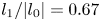 $l_1/|l_0| = 0.67$ in-between the two black lines. To further understand the slow evolution of Fourier space parameters of the secondary beam, figure 6 shows the temporal-frequency spectrograms computed using a Fourier transform for both experiments presented in figure 5, along with the corresponding DMD estimates of the triadic frequencies overlaid in white. The amplitude of the spectrograms are determined by
 \begin{equation} S_{\beta_{z}}(\omega, t) = \left\langle\left| \frac{1}{T_T}\int_{-\infty}^{+\infty}\beta_{z}(x,z,t') \,{\rm e}^{-{\rm i}2{\rm \pi} (\omega t')} W(t'-t; T_T)\, {\rm d} t' \right|^2\right\rangle_{w}, \end{equation}
where  $W(t'; T_T)$ is a Hamming window of non-dimensional width
  $T_T/T_0 = 39$. For the frame rate of 1 f.p.s., the highest resolvable frequency (shortest time period) is
  $\omega /N = 4.08$. Several windowing functions were tested, and were not found to significantly affect the spectrogram results. The angled brackets,
  $\langle \rangle _{w}$, again indicate that the results are averaged across the whole visualisation region. This underlying spectrogram, calculated using (3.4), reveals the details about the distribution of the frequency spectra for
  $\omega _1$ and
  $\omega _2$. In contrast, as we are only selecting the three dominant modes obtained from the DMD over short time intervals (
 $\delta t/T_0 = 3$), this methods approximates the underlying energy spectrum by a series of delta functions, allowing us to clearly see the slow-time evolution of these dominant modes.

Figure 6. Time–frequency spectra with spectral density computed by (3.4) and normalised by the total energy  $S_E = \sum _{z=0}^{H} S_{\beta _{z}}(\omega )^2$ for each instant in time. The dominant frequencies obtained from the DMD frequency decomposition are overlaid in white. (a) The same experiment shown in figure 5(a) (and also in figures 2 and 4) with a run time of
  $t_{end}/T_0 = 816$ and amplitude
  ${|l_0|A_0} = 0.200$. The white dashed lines are at the same times of the first six in figure 5(a) and indicate the times of the wavenumber spectrograms shown in figure 8. (b) The same experiment shown in figure 5(b), with a longer run time of
 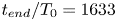 $t_{end}/T_0 = 1633$ and amplitude
  ${|l_0|A_0} = 0.200$. The subplot overlaid on (b) shows a transect in time at
  $t/T_0 = 452$, marked by the cyan and magenta arrows. Here we have plotted
  $\ln (S_{\beta _z} (\omega )/S_E)$ in cyan and
  $\ln (S_{\beta _z} (\omega _0 - \omega )/S_E)$ in magenta against
  $\omega /\omega _0$.
Both spectrograms in figures 6(a) and 6(b) show a clear peak at  $\omega _0/N = 0.62$ for all time, consistent with the imposed displacement from ASWaM. Both secondary beams emerging from the instability become visible at approximately
  $t/T_0 = 50$, with peaks in the spectra around
  $\omega _1/N \approx 0.23$ and
  $\omega _2/N \approx 0.39$, though subsequently these modulate on a slow time-scale throughout the duration of an experiment. The overlaid DMD frequency estimates match almost perfectly the three frequency peaks on the spectrogram, following the same pattern of slow modulations. Despite this modulation, the temporal triadic relationship
  $\omega _0 = \omega _1 + \omega _2$, is satisfied at all times for the frequencies obtained from the DMD. As noted previously, the triadic requirement is not built into the DMD analysis. Interestingly, a similar variation in frequency has been witnessed by both Bourget et al. (Reference Bourget, Dauxois, Joubaud and Odier2013) and Brouzet et al. (Reference Brouzet, Ermanyuk, Joubaud, Sibgatullin and Dauxois2016) in their experimental studies, however, the phenomenon was not the focus of their work.
In addition to the triadic frequencies, there are three other distinct frequency bands found in the time–frequency spectrograph. The band with the lowest frequency corresponds to  $\omega /N \approx 0$, which was also observed from the DMD and has already been discussed. The other two frequencies
  $\omega /N \approx$ 0.84 and
  $\omega /N \approx 1$ correspond to two different TWIs, given in (3.2), between
  $\mathbb {B}_0$ and either
  $\mathbb {B}_1$ or
  $\mathbb {B}_2$, respectively.
What is perhaps most striking from these time-frequency spectra is how, at certain points in time, there are multiple sets of  $\mathbb {B}_1$ and
  $\mathbb {B}_2$ associated with the instability. This is shown by the convergent ‘wisps’ on the
  $\omega _1/N$ and
  $\omega _2/N$ bands, where additional secondary beam pairs appear and merge with the continuous mode. This is highlighted for
  $t/T_0 = 452$ by the inset in figure 6(b). Here we have plotted
  $\ln (S_{\beta _z} (\omega )/S_E)$ in cyan and
  $\ln (S_{\beta _z} (\omega _0 - \omega )/S_E)$ in magenta against
  $\omega /\omega _0$. The presence of a spectrum of triadic relations here is evidenced by the strong correlation between the two traces, indicating that the triadic requirement
  $\omega _1 + \omega _2 = \omega _0$ persists across all the spectrum.
To analyse these frequency modulations further, figure 7 shows the real part of the dynamic modes from the DMD of the experiment presented in figure 4 over frames  $481 \leq t/T_0 \leq 483$ (panel (f)). Unlike its earlier counterpart in figures 2(c) and 2(d), where there was one distinct frequency and wavenumber pair for both
  $\mathbb {B}_1$ and
  $\mathbb {B}_2$, figures 7(c) and 7(d) show that, at this instant in time, TRI is occurring at two different locations over the height of the primary beam. For both of these modes, the signal is discontinuous across a transition region where the two out-of-phase wave beams deconstructively meet, highlighted by the black dashed rectangle in figure 7(d). Indeed, the presence of these separate beams is confirmed by splitting the domain in half and performing the DMD analysis separately on the two halves. For the upper half of the domain
  $\omega _1/N = 0.211$ and
 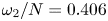 $\omega _2/N = 0.406$, while in the bottom half of the domain
  $\omega _1/N = 0.214$ and
  $\omega _2/N = 0.403$.

Figure 7. (a) The non-dimensional vertical gradient of the density perturbation  $\beta _z$ for the same panel shown in figure 4(f) at
  $t/T_0 = 481$. (b)–(d) The real part of the three pairs of dominant modes extracted using DMD over a time-window from
  $481 \leq t/T_0 \leq 483$. Specifically, (b)
  $\mathbb {B}_0$ with
  $\omega _0/N= 0.617$ (c)
  $\mathbb {B}_1$ with
  $\omega _1/N = 0.211$ (d)
  $\mathbb {B}_2$ with
  $\omega _2/N = 0.405$. The black dashed box in (d) indicates the region of discontinuity in the
  $\mathbb {B}_2$ beam.
The spatial dependence of the instability is highlighted further in figure 8, where the 3-D surface plots shows the horizontal components of the wave vectors  ${l_1}$ and
  ${l_2}$ as a function of height in the domain for six different instances in time, given by the white dashed lines on figure 6(a). The surface is defined by
 \begin{equation} S_{\beta_{z}^\ddagger}(l,z,t) = \left| \int_{-\infty}^{+\infty}\beta_{z}^\ddagger(x',z,t) \,{\rm e}^{-{\rm i}2{\rm \pi} l x} W(x' - x; X_X) \,{{\rm d}\kern0.7pt x}' \right|^2, \end{equation}
where  $W(x'; X_X)$ is a Hamming window of width
  $X_X = |l_0|x = 60.9$, spanning the full width of the domain. Here,
  $\beta _{z}^\ddagger (x, z, t)$ corresponds to the instantaneous vertical density perturbation gradient that has already been temporally filtered in Fourier space to remove the signal from
  $\omega _0$. The surface plots show (3.5) evaluated at each height in the domain to obtain the horizontal component of wavenumber
  $l_1$ and
  $l_2$. The contour plots behind show the corresponding frequency–wavenumber spectrogram. This is obtained by the 2-D Fourier transform (in
  $x$ and
  $t$)
$t$)
 \begin{align} S_{\beta_{z}^\ddagger}(\omega, l, t) \!=\! \left\langle\left| \frac{1}{T_T}\int\int_{-\infty}^{+\infty}\beta_{z}^\ddagger(x',z,t') \,{\rm e}^{-{\rm i}2{\rm \pi}(lx' + \omega t')} W(x'\!-\!x; X_X) W(t'\!-\!t; T_T) {{\rm d}\kern0.7pt x}' \, {\rm d}t' \right|^2\right\rangle_{z}\!\!, \end{align}
where the widths of the Hamming windows are given by  $T_T/T_0 = 39$ and
  $X_X = |l_0|x = 60.9$, and the subscript
  $z$ on the angle brackets shows that
  $S_{\beta _{z}^\ddagger }(\omega, l, t)$ is averaged over the height of the domain. The region of spatiotemporal discontinuity shown in physical space by the black dashed rectangle in figure 7(d) is clearly visible in wavenumber space in figure 8(f). The peak of the spectral isosurface in figure 8(f) corresponding to
  $l_2$, around mid-height in the domain, shows a shift in both the amplitude and value where the peak occurs. The presence of this discontinuous region indicates that two wave beams, of slightly different frequency and wavenumber, are destructively interfering with each other. Earlier, at
  $t/T_0 = 83$ in Figure 8(a) (corresponding to figure 4a) as the instability is developing, the triadic interaction is localised at the top of the domain, with little signal in the lower part (as here there is very low amplitude signal for both
  $l_1$ and
  $l_2$). The development of the subsequent panels in figure 8 show how the strength, location and the local values of
  $l_1$ and
  $l_2$ continuously shift over time. This spatial and temporal variation reveals that multiple resonant triads can be present in the domain simultaneously. This continuously varying range of wavenumbers explains why the grey region of experimentally obtained characteristic wavenumbers on figure 3 does not exactly fit the spatial triadic conditions of the underlying green branch of the loci.

Figure 8. Six surface plots corresponding to the first six snapshots in figure 4 (times also marked by the first six black lines in figure 5 and the white lines in figure 6), showing the distribution of  $l_1$ and
  $l_2$ over the non-dimensional height in the domain (
 $z/H$) calculated by (3.5): (a)
  $t/T_0 = 83$, (b)
  $t/T_0 = 180$, (c)
  $t/T_0 = 294$, (d)
  $t/T_0 = 347$, (e)
  $t/T_0 = 450$ and (f)
  $t/T_0 = 481$. Here the
  $\beta _z$ image sequence is first temporally filtered in Fourier space to remove the signal from
  $\mathbb {B}_0$, and thus we do not see a peak at
  $l_0$. Both the surface plot colour and the height of the peaks, show the power spectral density
  $S_{\beta _{z}^\ddagger }(l,z)$. The background plot then shows
  $l_1$ and
  $l_2$ at the same instant in time in the Fourier plane of horizontal wavenumber component and of frequency. This contour plot is defined by (3.6).
We speculate that the reason for these modulations, observed in both real and Fourier space, is due to the finite width of the primary wave beam. As a packet of energy in  $\mathbb {B}_1$ or
  $\mathbb {B}_2$ exits the underlying primary beam, the energy exchange between the triad is broken. The time taken for both these secondary beams to exit the spatial confines of
  $\mathbb {B}_0$ is dependant on the group velocities of the beams, which are functions of their wavenumbers, and the relative orientation of the beams determined by their frequencies. If the secondary beams are unable to extract sufficient energy before propagating out of the primary beam, the triad system will not be able to form a stable equilibrium and another triadic perturbation will grow in another location. Moreover, all the triadic beams are composed of a broadband wavenumber spectrum due to their finite width, as shown in figure 8. This introduces a range of group velocities in the secondary beams which will exit the underlying beam at different times, enhancing the unsteady transfer of energy.
In addition, the structure of the underlying  $\mathbb {B}_0$ varies across the height of the domain. As
  $\mathbb {B}_0$ propagates upwards through the tank, it decays due to viscosity, resulting in a broadening in spatial extent and reduction in amplitude (Fan & Akylas Reference Fan and Akylas2020). These combine to give considerable variation in both real and Fourier space over the height of the domain, where different locations will favour slightly different triadic perturbations. Indeed, as different perturbations grow, the secondary wave beams with very similar frequencies could interact with each other nonlinearly via the primary wave beam, generating a slow ‘beating’ effect. This interaction could cause the secondary beams to decay in some locations, whereas in others it causes a growth in amplitude, amplifying the effects of the modulations. Making the approximation that there is a single discrete set of parameters corresponding to the secondary wave beam for the whole domain is therefore an oversimplification that ignores the spatial variation of the instability.
4. Weakly nonlinear model construction
From the experimental results presented here, we believe that the unsteady behaviour of the instability is a function of the finite-width  $\varLambda _{0}$ of the primary beam
  $\mathbb {B}_0$. We therefore seek to understand this interaction in a 2-D context. We pursue this through the development of a 2-D weakly nonlinear model, which we refer to as
  $\mathcal {M}_{2\hbox{-}\textrm {D}}$. The goal here is to dissect the experiments and to isolate the dynamics that are observed experimentally, in order to improve the understanding of the system. A computational fluid dynamics (CFD) code would be an inappropriate choice to achieve this, as little would be learnt about the physical mechanisms governing the behaviour. In this section we detail the perturbation expansion used to develop the 2-D framework for the
  $\mathcal {M}_{2\hbox{-}\textrm {D}}$ model. Details of the numerical solution to the obtained system of equations are given in Appendix B.
Assuming a 2-D incompressible continuously stratified Boussinesq fluid in background hydrostatic balance with constant buoyancy frequency  $N$, the Boussinesq nonlinear equations of motion are given by
 \begin{gather} \varrho_0 \frac{{\rm D}\boldsymbol{u}}{{\rm D}t} ={-}\boldsymbol{\nabla} p - g\rho\boldsymbol{\hat{z}} + \mu {\nabla}^2\boldsymbol{u}, \end{gather}
 \begin{gather}\frac{{\rm D}\rho}{{\rm D}t}={-}w \frac{{\rm d}\bar{\rho}}{{\rm d}z}, \end{gather}
 \begin{gather}\boldsymbol{\nabla} \boldsymbol{\cdot} \boldsymbol{u} = 0, \end{gather}
where  $p$ is the dynamic pressure (set through the need to satisfy the incompressiblity condition (4.3)) and
  $\mu$ is the dynamic viscosity. Here, (4.1) is the momentum equation, whereas for this incompressible Boussinesq flow without mass diffusion (infinite Schmidt number, a reasonable approximation for salt in water) where we also neglect the transfer of mechanical energy to internal energy through viscous dissipation, the internal energy conservation (4.2) reduces to density being a materially conserved quantity. We note that for thermal stratification, whether in water or air, it would be inappropriate to ignore thermal diffusion but include viscosity.
Writing velocity in terms of the scalar stream function  $\boldsymbol {u} = \boldsymbol {\nabla } \times (\varPsi \hat {\boldsymbol {y}})$, this system can be reduced to
 \begin{gather} \frac{{\rm D}^2}{{\rm D}t^2} (\boldsymbol{\nabla}^2 \varPsi) - \frac{{\rm D}}{{\rm D}t}\nu \boldsymbol{\nabla}^2(\boldsymbol{\nabla}^2\varPsi) + N^2\frac{\partial^2\varPsi}{\partial x^2} = \frac{g}{\varrho_0}\left(\frac{\partial}{\partial x}\frac{{\rm D}}{{\rm D}t} - \frac{{\rm D}}{{\rm D}t}\frac{\partial}{\partial{x}}\right)\rho, \end{gather}
 \begin{gather}\frac{{\rm D}\rho}{{\rm D}t} ={-}\frac{\partial \varPsi}{\partial x}\frac{{\rm d}\bar{\rho}}{{\rm d}z}. \end{gather}
Details of the derivation of (4.4) are given in Appendix A. Here, we focus on (4.4), which represents the nonlinear momentum balance in terms of stream function and density. We seek the simplest form of the stream function and density that will describe the behaviour of TRI in a finite-width beam. Specifically we define
 \begin{gather} \varPsi = \tilde{\varPsi}(x, z, t)\, {\rm e}^{{\rm i} (\boldsymbol{k} \boldsymbol{\cdot} \boldsymbol{x} - \omega t)} + \textrm{c.c.}, \end{gather}
 \begin{gather}\rho = \tilde{\rho}(x, z, t)\, {\rm e}^{{\rm i}(\boldsymbol{k} \boldsymbol{\cdot} \boldsymbol{x} - \omega t)} + \textrm{c.c.}, \end{gather}
where  $\tilde {\varPsi }$ and
  $\tilde {\rho }$ are the reduced forms of the stream function and density, respectively, and c.c. represents the complex conjugate. Both
  $\tilde {\varPsi }$ and
  $\tilde {\rho }$ are given as functions of space and time because, based on the experimental results, the behaviour of TRI in a finite-width beam is spatiotemporally dependant.
We define the two non-dimensional parameters
 \begin{gather} \epsilon =|l_0||\tilde{{\xi}}_{00}|, \end{gather}
 \begin{gather}\gamma = (|l_0| L)^{{-}1}, \end{gather}
where  $|\tilde {{\xi }}_{00}|$ is the characteristic magnitude of the experimental amplitude associated with the primary beam
  $\mathbb {B}_0$ and
  $L$ is a characteristic length scale in the direction of
  $|\boldsymbol {c_g}|$ over which the amplitude of
  $\tilde {\varPsi }$ changes. Here,
  $\epsilon$ can be viewed as a non-dimensional measure of the experimental primary beam amplitude, which characterises the relative importance of the nonlinear
  $\boldsymbol {u} \boldsymbol {\cdot } \boldsymbol {\nabla }$ terms in the momentum and internal energy conservation equations. The spatial parameter
  $\gamma$ is then a non-dimensional distance over which we observe variations in the amplitude. When
  $L$ is sufficiently large, these changes depend only on viscosity
  $(L = \nu /|\boldsymbol {c_g}|)$. In the more limiting case of small
  $L = \varLambda _0$, (where
  $\varLambda _0$ is the primary beam width), we see changes occurring to secondary wave beams that are a function of the nonlinear interactions over the finite width of the primary beam. When considering viscous effects in oceanographic settings,
  $\gamma$ will be orders of magnitude smaller than
  $\epsilon$ as, at the scales of interest, the role of viscosity in the ocean can be considered negligible. Here, however, as experiments are inherently more viscous than similar motion patterns at oceanic scales, we retain the leading-order effects of viscosity. We restrict our attention to experimental parameters: low-amplitude
  $\epsilon \sim 10^{-2} \ll 1$, finite-width
  $\gamma \sim 10^{-2} \ll 1$, viscous beams
  $\gamma \sim 10^{-3} \ll 1$ and introduce re-scaled time and position through the four variables
 \begin{equation} \tau_\gamma = \gamma t, \quad {\zeta_x} = \gamma x, \quad {\zeta_z} = \gamma z, \quad \tau_\epsilon = \epsilon t. \end{equation}
As we shall see,  $\tau _\epsilon$ accounts for the ‘slow nonlinear time’ variations to the amplitude, whereas
  $\tau _\gamma$ governs the ‘slow advection time’ scale, the time for a packet of energy to cross the wave beam as opposed to the fast time associated with
  $\omega$. As, for the experiments, both
  $\epsilon \ll 1$ and
  $\gamma \ll 1$, these scaled times account for change over long-time periods. The spatial parameters
  ${\zeta _x}$ and
  ${\zeta _z}$ account for the gradual spatial variability of the wave beams in the domain. Utilising the dimensionless amplitude
  $\epsilon$, we rewrite the stream function in (4.6) as
 \begin{equation} \varPsi = \tilde{\varPsi}(x, z, t)\, {\rm e}^{{\rm i}(\boldsymbol{k} \boldsymbol{\cdot} \boldsymbol{x} - \omega t)} + \textrm{c.c.} = \epsilon\breve{\varPsi}(\tau_\gamma, {\zeta_x}, {\zeta_z}, \tau_\epsilon) \, {\rm e}^{{\rm i}(\boldsymbol{k} \boldsymbol{\cdot} \boldsymbol{x} - \omega t)} + \textrm{c.c.}, \end{equation}
where  $\tilde {\varPsi } = \epsilon \breve {\varPsi }$. We therefore require
  $|\breve {\varPsi }| \sim 1$ as we are interested in small perturbations to the flow. The ‘fast time’ is associated with the phase variations of the waves given by the wave frequency and is captured by the complex exponential wave form
  ${\rm e}^{{\rm i}(\boldsymbol {k} \boldsymbol {\cdot } \boldsymbol {x} - \omega t)} = {\rm e}^{{\rm i}\phi }$. As we are interested in the wave triad, we express the stream function as the summation in the same way as McEwan & Plumb (Reference McEwan and Plumb1977), by
 \begin{equation} \varPsi = \sum_{p=0}^{2}{\varPsi}_p = \sum_{p=0}^{2}\tilde{\varPsi}_p(x, z, t)\, {\rm e}^{{\rm i}\phi_p} + \textrm{c.c.} = \sum_{p=0}^{2}\epsilon\breve{\varPsi}_p(\tau_\gamma, {\zeta_x}, {\zeta_z}, \tau_\epsilon) \, {\rm e}^{{\rm i}\phi_p} + \textrm{c.c.}, \end{equation}
where the subscript  $p$ indicates a locally plane-wave approximation to
  $\mathbb {B}_0$,
  $\mathbb {B}_1$ or
  $\mathbb {B}_2$. Each wave phase
  ${\rm e}^{{\rm i}\phi _p}$ therefore represents the characteristic frequency and wavenumber contribution to
  $\mathbb {B}_p$. A similar set of expressions can be written for
  $\rho$ as a sum of
  $\epsilon \breve {\rho }_p \, {\rm e}^{{\rm i}\phi _p}$.
The superposition in (4.12), along with the equivalent for  $\rho$, is then substituted into the nonlinear (4.4) where, due to the separate space and time scales, the partial derivatives in (4.4) with respect to
  $(x,z,t)$ become
 \begin{gather} \frac{\partial \varPsi_p}{\partial x} = \epsilon \left({\rm i} l_p + \gamma \frac{\partial}{\partial {\zeta_x}} \right) \breve{\varPsi}_p \, {\rm e}^{{\rm i}\phi_p} + {\textrm{c.c.}}, \end{gather}
 \begin{gather}\frac{\partial \varPsi_p}{\partial z} = \epsilon \left({\rm i} m_p + \gamma \frac{\partial}{\partial {\zeta_z}} \right) \breve{\varPsi}_p \, {\rm e}^{{\rm i}\phi_p} + {\textrm{c.c.}}, \end{gather}
 \begin{gather}\frac{\partial \varPsi_p}{\partial t} = \epsilon \left({-}{\rm i} \omega_p + \gamma \frac{\partial}{\partial \tau_\gamma} + \epsilon \frac{\partial}{\partial \tau_{\epsilon}} \right) \breve{\varPsi}_p \, {\rm e}^{{\rm i}\phi_p} + {\textrm{c.c.}} \end{gather}
This substitution and following manipulations were performed with the aid of Mathematica (Wolfram Research Reference Wolfram Research2021) to ensure reliability of the lengthy algebraic manipulations required.
We note that at first order in  $\epsilon$, the right-hand side of (4.4) vanishes. Therefore, as the contributions from density on the right-hand side first appear at second order in
  $\epsilon$, it is valid to use the following linear relationship
 \begin{equation} \breve{\rho} ={-}\frac{l}{\omega} \frac{N^2 \varrho_0}{g} \breve{\varPsi}, \end{equation}
to remove density up until terms with a second order contribution from  $\epsilon$. The resultant expression obtained provides the Boussinesq viscous equations of motion solely as a function of
  $\varPsi$ that can be used to examine both linear and nonlinear dynamics between a triadic set of waves simply by collecting terms at orders of
  $\epsilon$ and
  $\gamma$.
The expression obtained at order  ${O}(\epsilon ^0 \gamma ^0)$ will be zero as these terms correspond to a state of rest. At order
  ${O}(\epsilon ^1 \gamma ^0)$, we recover the linear wave solution, with the nonlinearity in (4.4) vanishing and linear superposition applying such that the three waves propagate independently. Extracting terms with a common factor of
  ${\rm e}^{{\rm i}\phi _p}$, leaves
 \begin{equation} \frac{\omega_p}{N} = \frac{l_p}{\sqrt{(l_p^2 + m_p^2)}}, \end{equation}
which is the linear dispersion relationship for internal plane waves. Indeed, for a single nonlinear plane wave in the inviscid limit, the right-hand side of (4.4) vanishes whereas the left-hand side returns the dispersion relationship for non-trivial solutions, regardless of the wave amplitude.
We then collect terms at the next order,  ${O}(\epsilon ^1 \gamma ^1)$. We first examine the non-dimensional length scale
  $\gamma = (|l_0|\varLambda _0)^{-1}$, so considering spatial variations due to the finite width of the primary beam. Again, as
  $\epsilon$ is still at first order, the nonlinear terms in (4.4) cancel. Looking at the
  ${\rm e}^{{\rm i}\phi _p}$ terms, we obtain
 \begin{equation} 2 \epsilon \gamma \omega_p \kappa^2_p \frac{\partial \breve{\varPsi}_p}{\partial \tau_\gamma} = 2 \epsilon \gamma\left(l_p(\omega_p^2 - N^2)\frac{\partial \breve{\varPsi}_p}{\partial {\zeta_x}} + \omega^2_p m_p\frac{\partial \breve{\varPsi}_p}{\partial {\zeta_z}}\right), \end{equation}
which after some rearranging can be expressed as
 \begin{equation} \frac{\partial \breve{\varPsi}_p}{\partial \tau_\gamma} ={-} (\boldsymbol{c}_{g_p} \boldsymbol{\cdot} \boldsymbol{\nabla}_{\boldsymbol{{\zeta_x}}}) \breve{\varPsi}_p \rightarrow \frac{\partial \tilde{\varPsi}_p}{\partial t} ={-} (\boldsymbol{c}_{g_p} \boldsymbol{\cdot} \boldsymbol{\nabla}) \tilde{\varPsi}_p, \end{equation}
where  $\boldsymbol {\nabla }_{\boldsymbol {{\zeta _x}}} = (\partial /\partial {\zeta _x}, \partial /\partial {\zeta _z})$ and
  $\boldsymbol {\nabla } = (\partial /\partial x, \partial /\partial z)$. This linear advection equation shows that the stream function of each wave beam in the triad is advected at its respective group velocity. It is already well known that, for small-amplitude internal waves, the group velocity
  $\boldsymbol {c}_g$ is the velocity at which energy is transported (e.g. Sutherland Reference Sutherland2010). As energy scales approximately with
  $\varPsi ^2$, the fact that (4.17) shows that
  $\breve {\varPsi }$ is also advected by
  $\boldsymbol {c}_g$ is not altogether surprising.
We next consider spatial variations due to viscous effects, so  $\gamma = (|l_0| \nu )|\boldsymbol {c}_{g_0}|^{-1}$. When considering experimental parameters, this definition of
  $\gamma$ results in
  $\epsilon ^1 \gamma ^1 < \epsilon ^2$. Despite this, in both experimental and oceanographic settings the viscous decay of individual wave beams occurs irrespective of the nonlinear interactions, making it appropriate to consider their role in conjunction with the advection. Again, looking at terms with a common factor
  ${\rm e}^{{\rm i}\phi _p}$, we obtain the term
  $- \epsilon \gamma \kappa _p^4 |\boldsymbol {c}_{g_0}|\breve {\varPsi }_p /|l_0|$. Combining this term with (4.16) we obtain the viscous advection equation at
  ${O}(\epsilon ^1 \gamma ^1)$
 \begin{equation} \frac{\partial \tilde{\varPsi}_p}{\partial t} ={-}(\boldsymbol{c}_{g_p} \boldsymbol{\cdot} \boldsymbol{\nabla} ) \tilde{\varPsi}_p - \frac{\nu}{2}\kappa_p^2\tilde{\varPsi}_p, \end{equation}
which shows that the viscous decay of each beam scales as  $\kappa _p^2$. This advection equation in (4.18) is critical in providing the 2-D general framework in which we can examine the spatial effects of a finite-width beam. This equation forms the basis of our
  $\mathcal {M}_{2\hbox{-}\textrm {D}}$ model and details of how it is solved and its numerical implementation are addressed in Appendix B.
We next consider terms at order  ${O}(\epsilon ^2 \gamma ^0)$. Here, nonlinearity enters the problem and terms are no longer only associated with
  ${\rm e}^{{\rm i}\phi _p}$, but are also composed of cross-terms from
  $\boldsymbol {u} \boldsymbol {\cdot } \boldsymbol {\nabla }$ operator in (4.4) and have the form
  ${\rm e}^{{\rm i}(\phi _q + \phi _r)}$ when expressed in Fourier modes (where
  $p$,
$p$,  $q$ and
  $r$ are permutations of 0, 1 and 2). We consider a triad of wave beams satisfying resonance conditions (1.2). Using (4.14) to eliminate
  $\breve {\rho }$ from (4.4), at order
  ${O}(\epsilon ^2 \gamma ^0)$ we recover the nonlinear interactions found as ordinary differential equations (ODEs) in Bourget et al. (Reference Bourget, Dauxois, Joubaud and Odier2013) (although in our work the viscous decay has already been considered at
  ${O}(\epsilon ^1 \gamma ^1)$). Specifically, for the nonlinear interactions we obtain
 \begin{gather} \epsilon^2\frac{\partial \breve{\varPsi}_0}{\partial \tau_\epsilon} = \epsilon^2 I_0 \breve{\varPsi}_1 \breve{\varPsi}_2 \rightarrow \frac{\partial \tilde{\varPsi}_0}{\partial t} = I_0 \tilde{\varPsi}_1 \tilde{\varPsi}_2, \end{gather}
 \begin{gather}\epsilon^2\frac{\partial \breve{\varPsi}_1}{\partial \tau_\epsilon} = \epsilon^2 I_1 \breve{\varPsi}_0 \breve{\varPsi}_2^* \rightarrow \frac{\partial \tilde{\varPsi}_1}{\partial t} = I_1 \tilde{\varPsi}_0 \tilde{\varPsi}_2^*, \end{gather}
 \begin{gather}\epsilon^2\frac{\partial \breve{\varPsi}_2}{\partial \tau_\epsilon} = \epsilon^2 I_2 \breve{\varPsi}_0 \breve{\varPsi}_1^* \rightarrow \frac{\partial \tilde{\varPsi}_2}{\partial t} = I_2\tilde{\varPsi}_0 \tilde{\varPsi}_1^*, \end{gather}
where an asterisk indicates the complex conjugate and the interaction term is given as
 \begin{equation} I_p = \frac{l_q m_r - m_q l_r}{2\omega_p \kappa_p^2} \left[\omega_p(\kappa_q^2 - \kappa_r^2) + l_p N^2\left(\frac{l_q}{\omega_q} - \frac{l_r}{\omega_r}\right)\right]. \end{equation}
 Although is possible to extend this expansion to examine the higher order  ${O}(\epsilon ^2 \gamma ^1)$, this model captures the essence of the observed experimental behaviour and so inclusion of higher-order terms has not been pursued. By combining nonlinear interactions given in (4.19) with the advection equation (4.18), we have developed a framework for examining TRI that incorporates the 2-D spatial variation of a finite-width beam via the advection equation obtained at order
  ${O}(\epsilon ^1 \gamma ^1)$. This general framework is reassuringly consistent with the special case considered by Bourget et al. (Reference Bourget, Dauxois, Joubaud and Odier2013), where the instability is only considered as a function of time. This special case is first discussed in § 5.1. We then consider the results from the full the
  $\mathcal {M}_{2\hbox{-}\textrm {D}}$ model in § 5.2.
5. Weakly nonlinear behaviour
5.1. Zero-dimensional model results
As just highlighted, the coupled nonlinear interactions of (4.19) along with viscous attenuation can be recovered as a set of ODEs by considering the form  $\tilde {\varPsi }_p(t) \, {\rm e}^{{\rm i}\phi _p}$ in (4.4), where the slowly evolving reduced stream function is considered solely as a function of time. Indeed, this zero-dimensional (0-D) theory was first proposed by McEwan & Plumb (Reference McEwan and Plumb1977) and further developed by Koudella & Staquet (Reference Koudella and Staquet2006) and Bourget et al. (Reference Bourget, Dauxois, Joubaud and Odier2013).
Although the 0-D theory considers the ‘slow-time’ development of the amplitude of the beams, as noted by Sutherland (Reference Sutherland2013), it is still based upon the assumption that the waves are monochromatic in space and time. In the case of a finite-width beam becoming unstable to TRI, the secondary wave beams have a finite time with which to interact with the underlying primary beam. This limitation was addressed by Bourget et al. (Reference Bourget, Scolan, Dauxois, Le Bars, Odier and Joubaud2014), who adapted the coupled ODEs of the 0-D theory to examine the energy flux across a finite region of the primary wave beam. Using an energy balance, they define a 2-D control volume of width  $W_{0\hbox{-}{\rm D}}$ and length
  $L_{0\hbox{-}{\rm D}}$ over which the resonant beams can interact with the primary. Accounting for the energy fluxes in (from
  $\mathbb {B}_0$) and out (from all beams) of the control volume, the nonlinear interactions and viscous attenuation, the the 0-D theory becomes
 \begin{gather} \frac{{\rm d}\tilde{\varPsi}_0}{{\rm d} t} = I_0 \tilde{\varPsi}_1 \tilde{\varPsi}_2 - \nu \left(\frac{\kappa_0^2}{2} \right)\tilde{\varPsi}_0 + T, \end{gather}
 \begin{gather}\frac{{\rm d}\tilde{\varPsi}_1}{{\rm d} t} = I_1 \tilde{\varPsi}_0 \tilde{\varPsi}_2^* - \left(\frac{\nu \kappa_1^2}{2} + \frac{|\boldsymbol{c}_{g_1} \boldsymbol{\cdot} \boldsymbol{e}_{k_0}|}{2W_{0\hbox{-}{\rm D}}}\right)\tilde{\varPsi}_1, \end{gather}
 \begin{gather}\frac{{\rm d}\tilde{\varPsi}_2}{{\rm d} t} = I_2 \tilde{\varPsi}_0 \tilde{\varPsi}_1^* - \left(\frac{\nu \kappa_2^2}{2} + \frac{|\boldsymbol{c}_{g_2} \boldsymbol{\cdot} \boldsymbol{e}_{k_0}|}{2W_{0\hbox{-}{\rm D}}}\right)\tilde{\varPsi}_2, \end{gather}
where  $I_p$ is given in (4.20),
  $\boldsymbol {e}_{k_0}$ is a unit vector in the direction of
  $\boldsymbol {k}_0$ and the forcing term
  $T = |\boldsymbol {c}_{g_0}|(\tilde {\varPsi }_{{in}}^*\tilde {\varPsi }_{in} - \tilde {\varPsi }_0^*\tilde {\varPsi }_0)/(2L_{0\hbox{-}{\rm D}}\tilde {\varPsi }_0^*)$ in (5.1a), represents the energy flux for the primary wave beam through the control area with an incoming amplitude of
  $\tilde {\varPsi }_{{in}}$. We convert this input amplitude to the non-dimensional measure
  $(|l_0|^2|\tilde {\varPsi }_{{in}}|)/\omega _0 = |l_0|A_0$. The terms on the end of (5.1b) and (5.1c) represent the viscous decay within, and flux of energy out of, the control area. For the remainder of this article, we refer to the above set of spatially 0-D ODEs in (5.1), which we use to describe the energy exchange in TRI in the context of a finite-width beam, as the 0-D model
  $\mathcal {M}_{0\hbox{-}\textrm {D}}$.
The  $\mathcal {M}_{0\hbox{-}\textrm {D}}$ model is numerically integrated to examine its prediction for the development of the triad. To match the experimental set-up, the width
  $W_{0\hbox{-}{\rm D}}$ and length
  $L_{0\hbox{-}{\rm D}}$ of the interaction region are set to
  $\varLambda _{0}$ (defined in (2.3)) and
  $2\varLambda _{0}$, respectively (see Bourget et al. (Reference Bourget, Scolan, Dauxois, Le Bars, Odier and Joubaud2014) for details). The parameters for
  $\mathbb {B}_0$ are also kept consistent with the experimental ones. In the limit of
  $\mathcal {M}_{0\hbox{-}\textrm {D}}$,
  $\mathbb {B}_0$ reduces to
 \begin{equation} \mathbb{B}_0 = \{ \omega_0/N = 0.62, \quad \boldsymbol{k}_0/|l_0| = ({-}1, -1.32) \}. \end{equation}
 We are curious to see how varying the wavenumbers and frequencies of the secondary wave beams impact the evolution of the instability described by the  $\mathcal {M}_{0\hbox{-}{{\rm D}}}$. This is achieved by defining a resonant triad as
  $\mathbb {T}_\varPhi = \{\mathbb {B}_0, \mathbb {B}_{1_\varPhi }, \mathbb {B}_{2_\varPhi } \}$, where the subscript
  $\varPhi$ corresponds to a specific triadic configuration, obtained by changing the characteristic frequencies and wavenumbers of the secondary wave beams. We require that all the triadic configurations satisfy both the resonant condition (1.1) and dispersion (1.4), meaning all of the configurations lie exactly on the green curve in figure 3. For the
  $\mathcal {M}_{0\hbox{-}\textrm {D}}$ model, we consider configurations
  $\mathbb {T}_a$ and
  $\mathbb {T}_d$, marked by the blue circle and star on figure 3, respectively, with parameters listed in table 1.
Table 1. The input parameters of  $\mathbb {B}_{1_\varPhi }$ and
  $\mathbb {B}_{2_\varPhi }$ for each
  $\mathbb {T}_{\varPhi } = \{\mathbb {B}_0, \mathbb {B}_{1_\varPhi }, \mathbb {B}_{2_\varPhi }\}$, used in the
  $\mathcal {M}_{0\hbox{-}\textrm {D}}$ and
  $\mathcal {M}_{2\hbox{-}\textrm {D}}$ model. The wave vector locations of each secondary wave beam pair can be seen by the blue marks on figure 3. The corresponding non-dimensional frequency of the primary beam is
  $\omega _0/N = 0.617$.

The results of the numerical integration for the  $\mathcal {M}_{0\hbox{-}\textrm {D}}$ model are given in figure 9(a) and (b) for
  $\mathbb {T}_a$ and
  $\mathbb {T}_d$, respectively, across a range of five non-dimensional input amplitudes for the primary beam
  $0.053 \leq |l_0|A_0 \leq 0.105$. We note that these input amplitudes are about half of the input amplitudes from the wavemaker used in the experiments. This is because in the experiments there is a thin mixed layer, approximately
  $|l_0| D = 0.5$ thick (where
  $D$ is the depth in millimetres), which reduces the transmission of the waves by
  $\sim$50 % (Sutherland & Yewchuk Reference Sutherland and Yewchuk2004). As this layer is not present in either the
  $\mathcal {M}_{0\hbox{-}\textrm {D}}$ or
  $\mathcal {M}_{2\hbox{-}\textrm {D}}$ model, the input amplitudes required for instability in the models are considerably lower. When comparing amplitudes between the experiments, the
  $\mathcal {M}_{2\hbox{-}\textrm {D}}$ model and the
  $\mathcal {M}_{0\hbox{-}\textrm {D}}$ model, it is therefore best to compare the resultant beam amplitudes. One caveat of this, is that the
  $\mathcal {M}_{0\hbox{-}\textrm {D}}$ model is not a function of space, so the amplitude measure on the vertical axis on figure 9 (
 $|l_0||\tilde {{\xi }}_p|$, where
  $p = (0, 1, 2)$) is not directly comparable to the vertical axes of the experimental results shown in figure 5,
  $|l_0|\langle |\tilde {{\xi }}_p|\rangle _w$. To account for this we introduce
  $|l_0|\langle |\tilde {{\xi }}_0|\rangle _r$, the experimental amplitude of
  $\mathbb {B}_0$ averaged over the black domain
  $\langle \rangle _r$ in figure 2(b), to allow for comparison between the amplitudes of primary beam in the experiments and the
  $\mathcal {M}_{0\hbox{-}\textrm {D}}$ model. Details of the different amplitude are listed in table 2.

Figure 9. Results of the  $\mathcal {M}_{0-\textrm {D}}$ model by Bourget et al. (Reference Bourget, Scolan, Dauxois, Le Bars, Odier and Joubaud2014) given in (5.1) across a range of input amplitudes
  $0.053 \leq |l_0|A_0 \leq 0.105$. (a) Triad configuration
  $\mathbb {T}_a$ and (b) triad configuration
  $\mathbb {T}_d$. The parameters for these configurations are given in table 1.
Table 2. Details of the different non-dimensional measures of amplitude for clarity.

We first consider the general behaviour of the  $\mathcal {M}_{0\hbox{-}\textrm {D}}$ model, consistent between both figures 9(a) and 9(b). For the lowest input amplitude of
  $|l_0|A_0 = 0.053$, no instability occurs, so
  $|l_0||\tilde {{\xi }}_1|$ (red line) and
  $|l_0||\tilde {{\xi }}_2|$ (green line) remain zero whereas
  $|l_0||\tilde {{\xi }}_0|$ (blue line) remains at a constant amplitude of 0.046, after the initial growth period. There then exists a critical amplitude of the primary beam, above which TRI is observed. For
  $\mathbb {T}_a$ (figure 9a) this occurs when
  $|l_0||{\xi }_0| \geq$ 0.052, whereas for
  $\mathbb {T}_d$ (figure 9b), instability occurs when
  $|l_0||{\xi }_0| \geq$ 0.047. Although both of these limits are considerably lower than the experimental limit of
  $|l_0|\langle |\tilde {{\xi }}_0|\rangle _r \geq 0.095$, the
  $\mathcal {M}_{0\hbox{-}\textrm {D}}$ still captures the fact that there exists an amplitude threshold that must be surpassed before a finite-width beam exhibits TRI. We next note that, for all solutions where TRI is observed, the amplitude of
  $|l_0||\tilde {{\xi }}_0|$ always decays to the same asymptotic value, whereas the amplitudes of
  $|l_0||\tilde {{\xi }}_1|$ and
  $|l_0||\tilde {{\xi }}_2|$ asymptote at higher values as the input amplitude
  $|l_0|A_0$ is increased. Upon investigation, the asymptotic amplitude of
  $|l_0||\tilde {{\xi }}_0|$ after the initial decay is equal to the amplitude threshold for instability. Interestingly, for the larger input amplitudes, the approach to the equilibrium state takes the form of an underdamped nonlinear oscillator, shown by a small oscillation after the initial onset of the instability.
The difference between how the triad configurations  $\mathbb {T}_a$ and
  $\mathbb {T}_d$ affect the evolution of the instability is subtle. On inspection, figure 9(b) shows a quicker growth of the secondary beams for the same input amplitude as
  $\mathbb {T}_a$, a result that agrees with
  $\mathbb {T}_d$ having the lower amplitude threshold for instability. Strangely, despite this quicker growth, the resultant amplitudes of the secondary wave beams are smaller than in figure 9(a). This is counter-intuitive, as one would expect that a larger decay of the primary beam would result in larger amplitudes of the secondary beams. As the viscous decay along a beam scales with
  $\kappa ^2$, this lower value of the secondary beams might be due to greater viscous dissipation in
  $\mathbb {T}_d$, due to
  $\kappa _d > \kappa _a$. Indeed, when viscosity was turned off in the model (leaving only the inherent numerical dissipation), the amplitude of the secondary beams in
  $\mathbb {T}_d$ were found to have a larger resultant amplitude than those of
  $\mathbb {T}_a$.
Comparing figure 9 with the experimental results in figure 5, we see remarkably different behaviour in the evolution of the instability. For the  $\mathcal {M}_{0\hbox{-}\textrm {D}}$ model results, larger forcing engenders a significant decay in amplitude of the primary wave beam. This large decay of the primary beam is not observed experimentally, where the amplitude of the primary beam oscillates around a mean value comparable with that set by the forcing from the wavemaker. The most obvious difference between the two then arises in their description of the long-term development. The
  $\mathcal {M}_{0\hbox{-}\textrm {D}}$ model results predict that after the initial instability, the energy exchange between the triad saturates to a steady equilibrium, set by the nonlinear interaction term
  $I$. This is clearly not the case for the experimental results. The slow synchronous amplitude modulations seen experimentally reveal a continuous fluctuation in the energy exchange between the primary and the two secondary beams. As the
  $\mathcal {M}_{0\hbox{-}\textrm {D}}$ model does not consider the triadic interaction as a function of space, it is unable to describe the modulations witnessed experimentally.
5.2. Two-dimensional model results
We now consider the results from the  $\mathcal {M}_{2\hbox{-}\textrm {D}}$ model, where in each calculation we provide three domains, one for each triadic beam, with input parameters chosen to satisfy the triadic condition (1.2) and dispersion relation (1.4). Six triad configurations
  $\mathbb {T}_\varPhi = \{\mathbb {B}_0, \mathbb {B}_{1_\varPhi }, \mathbb {B}_{2_\varPhi } \}$ (where
  $\varPhi = a, b,\ldots, f$) are considered, with wavenumber vectors distributed across the solid green loci branch in figure 3 and parameters given in table 1. The parameters for
  $\mathbb {B}_0$ (common to all six triads), match the experiments and are given in (5.2a,b). Figure 10 shows the results of 36 calculations, where subplots (a)–(f) correspond to triad configurations
  $\mathbb {T}_{a}$ to
  $\mathbb {T}_{f}$, respectively, each shown with six input amplitudes,
  $|l_0|A_0$. Looking at all of the plots in figure 10, it is relatively easy to categorise three different patterns of behavioural evolution for the triads. The first evolutionary pattern of behaviour, observed for all the calculations using triad configurations
  $\mathbb {T}_a$ and
  $\mathbb {T}_b$ (shown by the blue circle and cross on figure 3), is when no growth of the secondary wave beams occur and the system remains as a single stable primary beam. The reason for this is twofold: both triad configurations satisfy (or nearly satisfy in the case of
  $\mathbb {T}_b$)
  $\kappa _1 / \kappa _0 \leq 1$ and both correspond to the smallest values of
  $\omega _1$ considered. Indeed, for input amplitudes that caused the other triadic configurations to become unstable, we found that no pairs with
  $\kappa _1 / \kappa _0 < 1$ generated TRI for the
  $\mathcal {M}_{2\hbox{-}\textrm {D}}$ model. This observation is further reinforced by our experiments: the grey shaded region on figure 3 shows that all observed triadic combinations of wave vectors satisfy
  $\kappa _1 / \kappa _0 > 1$. When
  $\kappa _1 / \kappa _0 < 1$, we have the condition
  $\kappa _1 < \kappa _0 < \kappa _2$. Thus, energy transfers to both the larger length scale (
 $\kappa _1$) and the smaller (
 $\kappa _2$). This is discussed in Bourget et al. (Reference Bourget, Scolan, Dauxois, Le Bars, Odier and Joubaud2014), who show that the theoretical linear growth rate for the
  $\mathcal {M}_{0\hbox{-}\textrm {D}}$ model is larger for the
  $\kappa _1 / \kappa _0 < 1$ configuration, only when
  $\varLambda _{0} > 7\lambda _{0}$. For wave beams narrower than this threshold (as in our experiments where
  $\varLambda _{0} \approx 3\lambda _{0}$), it is the triad configuration with
  $\kappa _1 / \kappa _0 > 1$ that is selected. The effect of having a smaller value of
  $\omega _1$ is discussed further in the following.

Figure 10. Amplitude plots generated using the 2-D weakly nonlinear  $\mathcal {M}_{2\hbox{-}\textrm {D}}$ model: (a)
  $\mathbb {T}_a$, (b)
  $\mathbb {T}_b$, (c)
  $\mathbb {T}_c$, (d)
  $\mathbb {T}_d$, (e)
  $\mathbb {T}_e$ and (f)
  $\mathbb {T}_f$. Each subplot shows a range input amplitudes for
  $\mathbb {B}_0$ between
  $0.053 \leq |l_0|A_0 \leq 0.105$. The difference between each subplot is the parameters for the secondary wave beams in each triad, given in table 1. The run time is
  $t_{{end}}/T_0 = 816$. The resultant non-dimensional amplitudes are averaged over the whole visualisation window
  $|l_0|\langle |\tilde {{\xi }}_p|\rangle _w$.
The second behaviour seen in figure 10, is when TRI occurs and the amplitudes of all beams undergo coupled modulations, similar to those seen experimentally in figure 5. This behaviour is observed for many of the calculations using triad configurations  $\mathbb {T}_c$ to
  $\mathbb {T}_f$. For these configurations, we see that an amplitude threshold must be surpassed before instability can occur. We note a very close agreement in the amplitude threshold between
  $\mathcal {M}_{2\hbox{-}\textrm {D}}$ and the experimental values. For the triad configurations
  $\mathbb {T}_c$ to
  $\mathbb {T}_f$, instability occurred when
  $|l_0|\langle |\tilde {{\xi }}_0|\rangle _w \geq$ 0.028, whereas experimentally
  $|l_0|\langle |\tilde {{\xi }}_0|\rangle _w \geq$ 0.029 triggered instability. We compare the resultant beam amplitudes as opposed to the input amplitudes
  $|l_0|A_0$ as, due to the mixed layer present in the experiments, the input amplitude required for instability is higher experimentally. We also note that for all of the calculations that become unstable, as we increase
  $|l_0|A_0$, not only do the secondary wave beam amplitudes increase, but also their growth also occurs at earlier times. This observation is consistent with the
  $\mathcal {M}_{0\hbox{-}\textrm {D}}$ model. We can measure this initial linear growth using the growth rate
  $\sigma$, of the form
  ${\rm e}^{\sigma t}$, to characterise how quickly the instability develops. This growth rate term will prove useful later.
Focusing on a specific calculation with coupled amplitude modulations, we consider triadic configuration  $\mathbb {T}_d$, forced at a non-dimensional input amplitude of
  $|l_0|A_0 = 0.092$ (figure 10d). Figure 11 shows six instantaneous images from this calculation obtained by the superposition of the three domains multiplied by their respective fast time and short length scales
  ${\rm e}^{{\rm i}\phi _p}$. Here we see the initial development of
  $\mathbb {B}_1$ occurring at the top of
  $\mathbb {B}_0$, where it grows in strength. (We note that the same calculation performed in a larger domain showed the generation region of
  $\mathbb {B}_1$ occurring at the same location, demonstrating that its growth is not due to boundary effects.) As with the experimental images in figure 4, due to the similar alignment and direction of
  $\boldsymbol {k}_0$ and
  $\boldsymbol {k}_2$,
  $\mathbb {B}_2$ is not obvious in this visualisation region as it propagates within the confines of
  $\mathbb {B}_0$. Over time,
  $\mathbb {B}_1$ grows in both amplitude and width before decaying in a quasi-periodic manner. Unlike the experimental results, however, its generation region remains approximately fixed and does not traverse the height of
  $\mathbb {B}_0$. By construction,
  $\omega _1$ and
  $\omega _2$ also remain fixed.

Figure 11. Sequence of images showing the superposition of the three domains in the model, using triad configuration  $\mathbb {T}_d$. Each domain is multiplied by its respective short length and fast time scales
  ${\rm e}^{{\rm i}\phi _p}$ and cast in terms of
  $\beta _z$ to allow for comparison with figure 4. The input amplitude for
  $\mathbb {B}_0$ is
  $|l_0|A_0 = 0.092$. The spatially averaged amplitude of each wave beam over time is shown in figure 10(d). The timing of each image is (a)
  $t/T_0 = 121$, (b)
  $t/T_0 = 184$, (c)
  $t/T_0 = 258$, (d)
  $t/T_0 = 547$, (e)
  $t/T_0 = 601$ and (f)
  $t/T_0 = 721$. These timings have been chosen to correspond to peaks and troughs in the amplitude modulation of the triad. The black line in (f) marks the length
  $\delta _1$, which defines the spatial distance over which
  $\mathbb {B}_1$ can extract energy from
  $\mathbb {B}_0$.
The final behavioural evolution seen in figure 10, most obvious for the largest input amplitude using  $\mathbb {T}_f$, is when the triadic system reaches a stable equilibrium, closely resembling the steady-state results from
  $\mathcal {M}_{0\hbox{-}\textrm {D}}$ shown in figure 9. Here, the amplitudes of the triadic beams do not exhibit any modulations and the triad quickly reaches a stable equilibrium, after a large, smooth decay in amplitude of the primary beam.
The only parameters being varied across these calculations in figure 10 are the frequencies and wavenumbers of the secondary beams in the triad and the amplitude of the primary beam. Consequently, this varying behavioural evolution of the triadic beams must be due to these changing parameters. Based on the dispersion relationship (1.4), a greater value of  $\omega _1$ results in a
  $\mathbb {B}_1$ beam with closer alignment to
  $\mathbb {B}_0$. This steeper angle leads to a greater spatial region over which a packet of energy propagating in
  $\mathbb {B}_1$ can extract energy from
  $\mathbb {B}_0$ and consequently an increased distance over which
  $\mathbb {B}_1$ can grow. This is shown schematically in figure 12. We define the lengths of these interaction regions for
  $\mathbb {B}_1$ and
  $\mathbb {B}_2$ as
  $\delta _1$ and
  $\delta _2$, respectively. Figure 13(a) shows the relationship between
  $\delta _1$ and
  $\omega _1$, together with the relationship between
  $\delta _2$ and
  $\omega _2$. The grey shading in the background marks the range of frequencies obtained experimentally.

Figure 12. Schematic showing the effect of different  $\omega _1$ and
  $\omega _2$ combinations on
  $\delta _1$ (red) and
  $\delta _2$ (green), the distances over which the secondary wave beams can extract energy with the primary beam before exiting the boundary.

Figure 13. (a) The non-dimensional interaction length of both  $\mathbb {B}_1$ and
  $\mathbb {B}_2$ with
  $\mathbb {B}_0$, as a function of non-dimensional frequency. The grey region in the background highlights the range of experimentally obtained frequencies. (b) The non-dimensional group velocity of both
  $\mathbb {B}_1$ (red) and
  $\mathbb {B}_2$ (green) as a function of non-dimensional frequency. The red and green shaded regions corresponds to the range of
  $|\boldsymbol {c}_g|$ possible for a fixed frequency due to a broadband wavenumber spectrum. Details of how these ranges are calculated are provided in the text. (c) The non-dimensional residence time
  $R_1/T_0$ (red) and
  $R_2/T_0$ (green) as a function of non-dimensional frequency, along with the non-dimensional inverse linear growth rates
  $(T_0 \sigma )^{-1}$, for most of the calculations shown in figure 10 and many others. Some of lower forcing amplitude calculations in figure 10 are not shown as their growth rates are too small (inverse growth rates too large). The style of the growth rate marker indicates the triad configuration tested (given in figure 3), whereas smaller solid dots are for other calculations not shown in figure 10). The colour of the marker indicates the behaviour of the simulation, characterised as no growth of secondary waves (magenta), amplitude modulations to the triadic beams (black) or steady equilibrium of all amplitudes in the triad (blue). The red and green shaded regions associated with the residence time are given from the range of
  $|\boldsymbol {c}_g|$ shown in (b).
As  $\omega _1$ increases, not only does
  $\delta _1$ increase,
  $|\boldsymbol {c}_{g_1}|$ also decreases, as shown in figure 13(b). A decrease in
  $|\boldsymbol {c}_{g_1}|$ also causes
  $\mathbb {B}_1$ to remain within the spatial confines of
  $\mathbb {B}_0$ for longer and hence increases the time in which it can extract energy. The red and green shaded regions on figure 13(b), associated with
  $|\boldsymbol {c}_{g_1}|$ and
  $|\boldsymbol {c}_{g_2}|$, respectively, mark the range of non-dimensional group velocities contained within the secondary beams due to their broadband spectrum. Although there is only one wavenumber vector
  $\boldsymbol {k}_1$ at each
  $\omega _1$ that can satisfy both dispersion (1.4) and the triadic resonant condition (1.2) (shown by the loci on figure 3), both
  $\mathbb {B}_1$ and
  $\mathbb {B}_2$ are beams that are broadly distributed over the wavenumber spectrum due to their finite width and so there will be exact triads selected from this distribution. A wavenumber distribution was clearly shown experimentally in figure 8, where a spectrum of
  $l_1$ and
  $l_2$ were observed, changing in both the physical location and duration of the experiment. As
  $|\boldsymbol {c}_{g_1}|$, defined in (3.1), is a function of wavenumber, this spectrum strongly impacts the range of group velocities present in the beam. The strength of the shading in figure 13(b) corresponds to the amplitude of the power spectrum for each wavenumber, obtained from Fourier transforming each secondary wave beam profile. The analytically calculated profile assumes a sinusoid with characteristic wavenumber given by the solid branch of the loci in figure 3 and width given by the geometry of the triad (assuming a primary beam width
  $\varLambda _{0}$), enclosed in a Gaussian envelope. Various windowing functions were tested and were not found to significantly alter the range of wavenumbers obtained.
The result of these two changing factors,  $\delta _q$ and
  $|\boldsymbol {c}_{g_q}|$ (where
  $q = 1$ or 2), shown in figure 13(a) and (b), respectively, are combined to form a residence time
  $R_q = \delta _q / |\boldsymbol {c}_{g_q}|$ that characterises how long each secondary wave beam spends within
  $\mathbb {B}_0$. The non-dimensional residence time, given as a function of frequency, is shown in figure 13(c). As
  $\omega _1$ increases,
  $R_1$ also increases. Although an increase in
  $\omega _1$ results in a decrease to
  $\omega _2$ and therefore a shallower angle for
  $\mathbb {B}_2$, as
  $\mathbb {B}_2$ and
  $\mathbb {B}_0$ are propagating the same direction, the residence time
  $R_2$ is always greater than
  $R_1$ and it is never the limiting factor in the interaction. This is shown by the consistently larger values of
  $R_2$ compared with
  $R_1$.
Overlaid on figure 13(c) are the inverse of the linear growth rates  $\sigma$ (given by the form
  ${\rm e}^{\sigma t}$), which are marked for all 36 calculations shown in figure 10 by the same
  $\mathbb {T}_{\varPhi }$ marker style as figure 3, along with many others for different calculations, marked with a solid dot. The linear growth rates are obtained by a linear fit on a logarithmic-linear plot to the initial growth of each simulation. The inverse growth rate can be viewed as a ‘development time’, that characterises how long the secondary beams take to grow. The colour of each mark indicates which behavioural evolution the calculation corresponds to. The magenta is used when no instability arose, the black markers represent those calculations with amplitude modulations and the blue marks indicate the calculations that achieved steady state. The behaviours of the calculations (shown with different style markers and larger size) can be verified from figure 10.
Figure 13 suggests why the  $\mathcal {M}_{2\hbox{-}\textrm {D}}$ model is so sensitive to the secondary wave parameters and why three different behavioural evolutions are observed across the triadic configurations tested. For the cases where no instability occurs, marked in magenta on figure 13(c), the development time of the secondary beams is greater than the residence time, meaning
  $\mathbb {B}_1$ propagates out of
  $\mathbb {B}_0$ before sufficient energy transfer can occur. This is case for all the input amplitudes shown in figures 10(a) and 10(b) using the triad configurations
  $\mathbb {T}_a$ and
  $\mathbb {T}_b$, where no growth of the secondary wave beams is observed. In this case,
  $R_1\sigma < 1$.
For the triad configurations and amplitudes that exhibited the quasi-periodic modulations in figure 10, their development times are marked in black. The majority of these points lie within the range of residence times for  $\mathbb {B}_1$. For these cases, therefore, the development time of the secondary wave beams is comparable with the time taken for
  $\mathbb {B}_1$ to propagate across
  $\mathbb {B}_0$. The secondary beams are able to grow but have insufficient time to saturate to a stable equilibrium, as wave perturbations will have moved out of the interaction region before this can occur. Moreover, due to the range of group velocities present in the beam, energy will be leaving the primary beam at different times, enhancing the modulations. For these cases,
  $R_1\sigma \approx 1$. Using this
  $R_1\sigma$ measure allows us to account for the input amplitude of the primary beam (which affects
  $\sigma$). For example, for the calculations marked with solid dots at low values of
  $\omega _1$, the input amplitude was significantly increased in order to get the secondary beams to grow.
The final behavioural evolution, observed for the higher-amplitude input in figure 10(e) and 10(f), is when the secondary beams grow and no modulations are observed; rather we see a smooth, rapid decay of the primary beam and the system reaching a steady state. For these cases, where  $R_1\sigma > 1$, the development times (marked by the blue triangle and cross) are sufficiently short compared with the range of residence times
  $R_1$. This means
  $\mathbb {B}_1$ is able to extract sufficient energy from the primary beam to reach a steady equilibrium (set by the value of the nonlinear interaction term
  $I_p$) before exiting the underlying
  $\mathbb {B}_0$. This reflects how the system would act in the limit of a plane wave, where the triadic interactions occur infinitely over space and time and the residence time is always greater than the development time.
6. Discussion and conclusions
Novel experimental results have shown that when TRI arises in a finite-width internal gravity wave beam, the physical regions containing the secondary wave beams continue to move around over long time scales without reaching a steady equilibrium. By isolating the beams of interest, we have found that the amplitudes of the triadic system fluctuate by  $\pm$55
 $\%$ of their mean value. We note that as energy scales with the square of the amplitude, these fluctuations are even more significant. Analysis using DMD and Fourier methods further reveals fluctuations in the Fourier space parameters of the secondary beams.
Using our  $\mathcal {M}_{2\hbox{-}\textrm {D}}$ model, we have isolated the weakly nonlinear dynamics of a single triad in a generalised spatiotemporal 2-D framework and thus explained the conditions under which certain triad configurations result in these amplitude fluctuations. The model reveals the sensitivity of the instability to the properties of the secondary waves and how, in the context of a finite-width beam, the spatiotemporal configuration of the triad plays a fundamental role in the evolution of the instability. The
  $\mathcal {M}_{2\hbox{-}\textrm {D}}$ model shows that when the development time has a time scale comparable to the duration of residence of a wave packet, the secondary beams are able to grow but are unable to extract sufficient energy to reach a saturated equilibrium state, resulting in continuous amplitude modulations. This phenomenon is also seen experimentally, yet in the experiments there is present a whole range of perturbations to the underlying flow. The triad configuration is dependant on the local structure of
  $\mathbb {B}_0$ and perturbations to the background stratification and, accordingly, preferential selection of triads is locally determined. As one triadic interaction decays, another forms, but this time at a different physical location with new secondary beam properties. This explains why, experimentally, modulations are observed not only in physical space but also in Fourier space. Unlike in the experiments, in the
  $\mathcal {M}_{2\hbox{-}\textrm {D}}$ model calculations presented here, the interaction region of the triad does not move in physical space, because by construction,
  $\mathbb {B}_1$ and
  $\mathbb {B}_2$ have fixed frequencies and wavenumbers and this causes growth in a specific location. Further work (not reported here; see Grayson (Reference Grayson2021)) suggests that when a number of different triad configurations are present in the
  $\mathcal {M}_{2\hbox{-}\textrm {D}}$ model, modulations of the secondary beams are also witnessed in both physical and Fourier space.
Although not detailed in this article, the ratios of  $1.6 \leq \kappa _1/\kappa _0 \leq 3.2$ and
 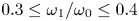 $0.3 \leq \omega _1/\omega _0 \leq 0.4$ observed in our experiments are consistent with those predicted by the theoretical maximum growth rate for a viscous fluid, as outlined by Bourget et al. (Reference Bourget, Dauxois, Joubaud and Odier2013). In the limit of
  $\nu \to 0$ (a situation approximating the ocean where the effects of viscosity are often neglected), the wavenumber for maximum growth rate asymptotes to infinity, whereas the frequencies tend towards the subharmonic:
  $\omega _1/\omega _0 \approx \omega _2/\omega _0 \approx \omega _0/2$.
In this limit we may expect two things to occur. First, due to this asymptotic theoretical growth rate, we may expect secondary beams with extremely broad-banded peaks producing a broad spectrum of high wavenumber components. However, in their numerical investigation into TRI for horizontally periodic modes, Sutherland & Jefferson (Reference Sutherland and Jefferson2020) find that in the case of  $\nu \to 0$ the bandwidths of their secondary beams are of similar width to those found in our experiments presented here. Second, in this inviscid limit, the solution may jump to the central branch on the loci shown in figure 3. As mentioned earlier, when including viscous effects, Bourget et al. (Reference Bourget, Scolan, Dauxois, Le Bars, Odier and Joubaud2014) calculate that this transition will not occur until approximately
  $\varLambda _0 > 7\lambda _0$. However, for the inviscid regime, they show that this width limit on the primary beam reduces and secondary waves of both smaller and larger length scales (
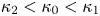 $\kappa _2 < \kappa _0 < \kappa _1$) may be selected. Sutherland & Jefferson (Reference Sutherland and Jefferson2020) do not witness this transition due to the confined vertical geometry preventing these larger length scales from being observed.
In the oceanographic context, rotation and nonlinear stratifications play a role in how TRI manifests. Considering non-uniform stratifications, Gayen & Sarkar (Reference Gayen and Sarkar2013) cite this instability as a source of significant energy transfer to subharmonic motions in the upper ocean pycnocline. Introducing rotation, Varma & Mathur (Reference Varma and Mathur2017) demonstrate how strong nonlinear effects are expected from triads with two modes at near-inertial frequency. Further theoretical work by Richet et al. (Reference Richet, Chomaz and Muller2018) and observations by Mackinnon et al. (Reference Mackinnon, Alford, Sun, Pinkel, Zhao and Klymak2013) show that around the critical latitude of 29 $^{\circ }$, triad interactions involving the primary internal tide and two near-inertial waves are important dissipation mechanism (Karimi & Akylas Reference Karimi and Akylas2017). Although the evolution of this near-inertial TRI around the critical latitude will be influenced by significantly more components than the dynamics isolated in this work, it raises the question as to whether similar dynamics can be found due to the variations in the residence time and growth rates of the waves we know to occur around these latitudes.
Although the direct applicability of our work to the ocean is limited, the implications of the failure of a steadily forced weakly nonlinear system to reach an equilibrium state is of profound importance. That we have demonstrated the establishment of long-lasting aperiodic modulations of the system both experimentally and using a reduced weakly nonlinear model is fundamental. We show that secondary waves can be produced for triads that do not correspond to the linear maximal growth rate; rather, the nonlinear interactions are able to pump energy into a host of alternative triad combinations. A key element of this non-equilibrium behaviour arises when the residence time of a packet of energy within a finite-width beam matches the inverse growth rate. This possibility of matching time scales, which is available in a finite-width beam, is lost in the limit of a plane wave.
Acknowledgements
For the purpose of open access, the authors have applied a Creative Commons Attribution (CC BY) licence to any Author Accepted Manuscript version arising from this submission.
Funding
KMG acknowledges support from an Natural Environmental Research Council (NERC) studentship (grant no. NE/L002507/1) and from an Engineering and Physical Sciences Research Council (EPSRC) fellowship (grant no. EP/W522600/1).
Declaration of interests
The authors report no conflicts of interest.
Appendix A
This appendix details how (4.4) is derived. We take the curl of the 2-D momentum equations (4.1) to eliminate pressure, leaving a form of the vorticity equation
 \begin{equation} \frac{\partial}{\partial{x}}\left(\varrho_0\frac{{\rm D}w}{{\rm D}t} +\rho g - \mu \nabla^2 w\right) -\frac{\partial}{\partial{z}}\left(\varrho_0\frac{{\rm D}u}{{\rm D}t} - \mu \nabla^2 u\right) =0. \end{equation}
Substituting  $\boldsymbol {u} = \boldsymbol {\nabla } \times (\varPsi \hat {\boldsymbol {y}})$ then dividing through by
  $\varrho _0$ and simplifying allows (A1) to be rewritten as
 \begin{equation} \frac{{\rm D}}{{\rm D}t} (\nabla^2 \varPsi) + \frac{g}{\varrho_0}\frac{\partial \rho}{\partial{x}} - \nu \nabla^2(\nabla^2\varPsi) = 0. \end{equation}
The material derivative of (A2) yields
 \begin{equation} \frac{{\rm D}^2}{{\rm D}t^2} (\nabla^2 \varPsi) + \frac{g}{\varrho_0}\frac{{\rm D}}{{\rm D}t}\frac{\partial \rho}{\partial{x}} - \frac{{\rm D}}{{\rm D}t}\nu \nabla^2(\nabla^2\varPsi) = 0. \end{equation}
 Differentiating (4.2) with respect to  $x$ and substituting for
  $\boldsymbol {u}$ and the buoyancy frequency gives
 \begin{equation} \frac{g}{\varrho_0}\frac{\partial}{\partial x}\frac{{\rm D}\rho}{{\rm D}t} - N^2\frac{\partial^2\varPsi}{\partial x^2}= 0. \end{equation}
 As both (A3) and (A4) have a similar form for the derivatives of  $\rho$, we equate them to reveal
 \begin{equation} \frac{{\rm D}^2}{{\rm D}t^2} (\nabla^2 \varPsi) - \frac{{\rm D}}{{\rm D}t}\nu \nabla^2(\nabla^2\varPsi) + N^2\frac{\partial^2\varPsi}{\partial x^2}= \frac{g}{\varrho_0}\left(\frac{\partial}{\partial x}\frac{{\rm D}}{{\rm D}t} - \frac{{\rm D}}{{\rm D}t}\frac{\partial}{\partial{x}}\right)\rho. \end{equation}
This then forms (4.4).
Appendix B
This appendix details the development of the  $\mathcal {M}_{2\hbox{-}\textrm {D}}$ numerical model. We solve the advection equation (4.18) using a monotonic second-order upwind finite volume scheme. The finite volume method discretizes the governing equations into rectangular control volumes around each node and the advective fluxes,
  $F$ are evaluated across the upwind faces. The advection velocity is given by the group velocity. We consider three numerical domains, one for each beam, with fixed Fourier components. This is sufficient to capture the amplitude modulations observed in our experiments, though it excludes frequency and wavenumber fluctuations seen experimentally in the secondary wave beams.
We define each domain used to advect the reduced stream function  $\tilde {\varPsi }_p$ in (4.18) as
  $\tilde {\mathbb {B}}_p$. The volume flux,
  $F$, is calculated using the two upstream values of the reduced stream function (here we drop the subscript
  $p$ for clarity)
 \begin{equation} \left.\begin{array}{c}
F_{w} = c_{g_x} \tilde{\varPsi}_{w}, \quad \textrm{where} \
\tilde{\varPsi}_{w} = \begin{cases} \tilde{\varPsi}_{W} +
\dfrac{\varUpsilon_{wW}}{2} (\tilde{\varPsi}_{W} -
\tilde{\varPsi}_{WW}) & \text{for } c_{g_x} > 0,
\rightarrow\\ \tilde{\varPsi}_{M} +
\dfrac{\varUpsilon_{wM}}{2} (\tilde{\varPsi}_{M} -
\tilde{\varPsi}_{E}) & \text{for } c_{g_x} < 0, \leftarrow
\end{cases} \\ F_{e} = c_{g_x}
\tilde{\varPsi}_{e}, \quad \text{where} \
\tilde{\varPsi}_{e} = \begin{cases} \tilde{\varPsi}_{M} +
\dfrac{\varUpsilon_{eM}}{2} (\tilde{\varPsi}_{M} -
\tilde{\varPsi}_{W}) & \textrm{for} \ c_{g_x} > 0,
\rightarrow \\ \tilde{\varPsi}_{E} +
\dfrac{\varUpsilon_{eE}}{2} (\tilde{\varPsi}_{E} -
\tilde{\varPsi}_{EE}) & \text{for} \ c_{g_x} < 0,
\leftarrow \end{cases} \\ F_{n} =
c_{g_z} \tilde{\varPsi}_{n}, \quad \textrm{where} \
\tilde{\varPsi}_{n} = \begin{cases} \tilde{\varPsi}_{M} +
\dfrac{\varUpsilon_{nM}}{2} (\tilde{\varPsi}_{M} -
\tilde{\varPsi}_{S}) & \text{for} \ c_{g_z} > 0, \uparrow
\\ \tilde{\varPsi}_{N} +
\dfrac{\varUpsilon_{nN}}{2}(\tilde{\varPsi}_{N} -
\tilde{\varPsi}_{NN}) & \text{for} \ c_{g_z} < 0,
\downarrow \end{cases} \\ F_{s} =
c_{g_z} \tilde{\varPsi}_{s}, \quad \textrm{where}\
\tilde{\varPsi}_{s} = \begin{cases} \tilde{\varPsi}_{S} +
\dfrac{\varUpsilon_{sS}}{2} (\tilde{\varPsi}_{S} -
\tilde{\varPsi}_{SS}) & \text{for} \ c_{g_z} > 0, \uparrow
\\ \tilde{\varPsi}_{M} +
\dfrac{\varUpsilon_{sM}}{2} (\tilde{\varPsi}_{M} -
\tilde{\varPsi}_{N}) & \text{for} \ c_{g_z} <
0, \downarrow \end{cases} \end{array}\right\}
\end{equation}
\begin{equation} \left.\begin{array}{c}
F_{w} = c_{g_x} \tilde{\varPsi}_{w}, \quad \textrm{where} \
\tilde{\varPsi}_{w} = \begin{cases} \tilde{\varPsi}_{W} +
\dfrac{\varUpsilon_{wW}}{2} (\tilde{\varPsi}_{W} -
\tilde{\varPsi}_{WW}) & \text{for } c_{g_x} > 0,
\rightarrow\\ \tilde{\varPsi}_{M} +
\dfrac{\varUpsilon_{wM}}{2} (\tilde{\varPsi}_{M} -
\tilde{\varPsi}_{E}) & \text{for } c_{g_x} < 0, \leftarrow
\end{cases} \\ F_{e} = c_{g_x}
\tilde{\varPsi}_{e}, \quad \text{where} \
\tilde{\varPsi}_{e} = \begin{cases} \tilde{\varPsi}_{M} +
\dfrac{\varUpsilon_{eM}}{2} (\tilde{\varPsi}_{M} -
\tilde{\varPsi}_{W}) & \textrm{for} \ c_{g_x} > 0,
\rightarrow \\ \tilde{\varPsi}_{E} +
\dfrac{\varUpsilon_{eE}}{2} (\tilde{\varPsi}_{E} -
\tilde{\varPsi}_{EE}) & \text{for} \ c_{g_x} < 0,
\leftarrow \end{cases} \\ F_{n} =
c_{g_z} \tilde{\varPsi}_{n}, \quad \textrm{where} \
\tilde{\varPsi}_{n} = \begin{cases} \tilde{\varPsi}_{M} +
\dfrac{\varUpsilon_{nM}}{2} (\tilde{\varPsi}_{M} -
\tilde{\varPsi}_{S}) & \text{for} \ c_{g_z} > 0, \uparrow
\\ \tilde{\varPsi}_{N} +
\dfrac{\varUpsilon_{nN}}{2}(\tilde{\varPsi}_{N} -
\tilde{\varPsi}_{NN}) & \text{for} \ c_{g_z} < 0,
\downarrow \end{cases} \\ F_{s} =
c_{g_z} \tilde{\varPsi}_{s}, \quad \textrm{where}\
\tilde{\varPsi}_{s} = \begin{cases} \tilde{\varPsi}_{S} +
\dfrac{\varUpsilon_{sS}}{2} (\tilde{\varPsi}_{S} -
\tilde{\varPsi}_{SS}) & \text{for} \ c_{g_z} > 0, \uparrow
\\ \tilde{\varPsi}_{M} +
\dfrac{\varUpsilon_{sM}}{2} (\tilde{\varPsi}_{M} -
\tilde{\varPsi}_{N}) & \text{for} \ c_{g_z} <
0, \downarrow \end{cases} \end{array}\right\}
\end{equation}
where the compass indexing is shown in the schematic in figure 14 and  $\varUpsilon$ is the flux limiter. The form of the flux equation in (B1) is chosen based on the direction of the group velocity in that domain. For every domain
  $\tilde {\mathbb {B}}_p$, the calculation is performed once on the real part of
  $\tilde {\varPsi }$ and once on the imaginary, with
  $\varUpsilon$ common to both calculations. The subscript on
  $\varUpsilon$ indicates the direction of the flux, as the flux limiter will change depending on the direction of flow. We use the ‘min-mod’ function (Versteeg & Malalasekera Reference Versteeg and Malalasekera2007)
 \begin{equation} \varUpsilon(r) = \max[0, \min(1, r)], \end{equation}
where  $r$ is given as the ratio of the downstream to upstream gradient. For four different flow directions,
  $r$ (following the same subscript notation as (B1)
  $r$ is given as
 \begin{equation} \left.\begin{array}{c} r_{wW} = \dfrac{\tilde{\varPsi}_M - \tilde{\varPsi}_W}{\tilde{\varPsi}_W - \tilde{\varPsi}_{WW}} \quad \textrm{for} \ c_{g_x} > 0, \rightarrow \\ r_{eE} = \dfrac{\tilde{\varPsi}_M - \tilde{\varPsi}_E}{\tilde{\varPsi}_E - \tilde{\varPsi}_{EE}} \quad \text{for} \ c_{g_x} < 0, \leftarrow \\ r_{nN} =\dfrac{\tilde{\varPsi}_M - \tilde{\varPsi}_N}{\tilde{\varPsi}_N - \tilde{\varPsi}_{NN}} \quad \text{for} \ c_{g_z} > 0, \downarrow \\ r_{sS} = \dfrac{\tilde{\varPsi}_M - \tilde{\varPsi}_S}{\tilde{\varPsi}_S - \tilde{\varPsi}_{SS}} \quad \text{for} \ c_{g_z} < 0. \uparrow \end{array}\right\} \end{equation}
Depending of the gradient ratio in  $r$,
$r$,  $0 \leq \varUpsilon \leq 1$. A monotonic scheme is achieved by reducing (
 $0 < \varUpsilon < 1$) or eliminating (
 $\varUpsilon = 0$) the second-order contributions where necessary. Equation (B2) is calculated for both the real and imaginary domain and the most restrictive value (the one that most reduces the second-order contributions) is used for both the real and imaginary flux calculations.

Figure 14. Sketch outlining the numerical advection domain  $\tilde {\mathbb {B}}_0$. The left-hand grid shows the full domain, including the bottom boundary forcing of the wavemaker, which is given by the sinusoid envelope in (2.2). The two outer grid layers required for the second-order scheme are shown in blue. In this domain
  $\boldsymbol {c}_{g_0}$ is directed to the north-west, meaning the advection of the complex
  $\tilde {\varPsi }_0$ is to the north-west, indicated by the black arrows pointing north-west. The enlarged view panel on the right shows the close-up of one control volume. For advection,
  $\tilde {\varPsi }_0$ is spilt into its real and imaginary parts. The front domain represents the real part of the flux, whereas the back faded domain represents the imaginary part of the flux.
The left-hand panel in figure 14 shows the full domain  $\tilde {\mathbb {B}}_0$. The enlarged view panel on the right shows one finite volume, marked by the red dashed square, where the flux across the north and west boundaries are given in (B1). The front and back grids represent the real and imaginary parts of
  $\tilde {\varPsi }_0$ respectively. The value of the stream function at the central node
  $\tilde {\varPsi }_{M}$ is updated by
 \begin{equation} \tilde{\varPsi}_{M}^{{{\dagger}}} \!=\! \tilde{\varPsi}_M^{i} \!+\! {\rm \Delta} t \left(- \boldsymbol{\nabla} \boldsymbol{\cdot} \boldsymbol{c}_{g_0} \tilde{\varPsi}_M^i - \frac{\nu}{2}\kappa_0^2\tilde{\varPsi}_M^i\right) \!=\! \tilde{\varPsi}_{M}^{i} \!+\! {\rm \Delta} t \left(\frac{F_{w}^i \!-\! F_{e}^i}{{\rm \Delta} x} + \frac{F_{s}^i - F_{n}^i}{{\rm \Delta} z} - \frac{\nu}{2}\kappa_0^2\tilde{\varPsi}_M^i \right), \end{equation}
where  ${\rm \Delta} t$ is the time-step and the superscripts
  $i$ and
  ${\dagger}$ represent the value of
  $\tilde {\varPsi }$ before and after advection, respectively. For the scheme to remain numerically stable, we limit
  ${\rm \Delta} t$, to satisfy the CFL condition. To account for the complex value of
  $\tilde {\varPsi }$, (B4) is performed once of the real part and once on the imaginary. The resulting values are recombined to produce a full complex valued
  $\tilde {\varPsi }_{M}^{{\dagger} }$.
Each  $242 \times 82$ domain
  $\tilde {\mathbb {B}}_p$ matches the aspect ratio of the experimental visualisation window. The non-dimensional grid spacing,
  $|l_0|{\rm \Delta} x = |l_0|{\rm \Delta} z = 0.25$, is much finer than the smallest wavelength considered. At every time step, random complex background noise of magnitude
  $10^{-7} \delta \, \textrm {e}^{\textrm {i}(2{\rm \pi} \vartheta )}$ is added to each cell in every domain. Both
  $\delta$ and
  $\vartheta$ are independent random numbers spanning the range
  $[0,\ 1]$, giving a mean magnitude of the order
  $5 \times 10^{-8}$ with a uniformly distributed phase angle. Without the addition of a perturbation, the instability would not be triggered. For the boundaries corresponding to outgoing waves, standard non-reflecting boundary conditions are used. For the incoming boundaries, small-amplitude complex noise of the same structure as the background noise is advected into the domain.
The bottom boundary forcing of the wavemaker is imposed in domain  $\tilde {\mathbb {B}}_0$. The boundary condition is given by the envelope of the experimental forcing, which is obtained by removing the fast time forcing,
  $\textrm {e}^{\textrm {i}\phi _0}$, from (2.2) and (2.4). This boundary condition for
  $\tilde {\mathbb {B}}_0$ is shown in figure 14 in blue. We implement a prescribed displacement given by the complex-valued vertical amplitude
  $\mathcal {A}_0 = A_0\, \textrm {e}^{\textrm {i}(2{\rm \pi} \varphi )}$, where
  $\varphi$ is a constant phase angle within the range
  $[0,\ 1]$. At each time step, after each domain is advected at its respective group velocity, the nonlinear interactions (4.19) are calculated.
The nonlinear interactions are included by converting (4.19) into the numerical format
 \begin{gather} \tilde{\varPsi}_{0}^{i+1} = \tilde{\varPsi}_{0}^{{{\dagger}}} + {\rm \Delta} tI_0 \tilde{\varPsi}_{1}^{{{\dagger}}} \tilde{\varPsi}_{2}^{{{\dagger}}}, \end{gather}
 \begin{gather}\tilde{\varPsi}_{1}^{i+1} = \tilde{\varPsi}_{1}^{{{\dagger}}} + {\rm \Delta} tI_1 \tilde{\varPsi}_{0}^{{{\dagger}}} \tilde{\varPsi}_{2}^{{{\dagger}}*}, \end{gather}
 \begin{gather}\tilde{\varPsi}_{2}^{i+1} = \tilde{\varPsi}_{2}^{{{\dagger}}} + {\rm \Delta} tI_2 \tilde{\varPsi}_{0}^{{{\dagger}}} \tilde{\varPsi}_{1}^{{{\dagger}}*}, \end{gather}
where  $\tilde {\varPsi }_p$ corresponds to every cell in domain
  $\tilde {\mathbb {B}}_p$ and
  ${\dagger}$ and
  $i+1$, respectively, represent the values of
  $\tilde {\varPsi }_p$ in each domain after advection (B4) and at time
  $t + {\rm \Delta} t$ after the nonlinear interactions are calculated. As the interaction coefficient is applied to the whole domain, there is no need to distinguish here the different cells using compass indexing.


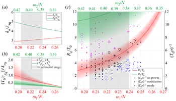


 Open access