


1. Introduction
The study of mass transfer in confined geometries is extremely important in many engineering and biological systems. In the context of geological  ${\rm CO}_{2}$ sequestration, carbon dioxide is injected into subsurface reservoirs, leading to the formation of elongated bubbles that can either be trapped, move or interact with the solid matrix (e.g. Rathnaweera, Ranjith & Perera Reference Rathnaweera, Ranjith and Perera2016; Soulaine et al. Reference Soulaine, Roman, Kovscek and Tchelepi2018; Li, Garing & Benson Reference Li, Garing and Benson2020). The presence of
  ${\rm CO_2}$ has the effect of increasing the acidity of the in situ brine, boosting a series of chain reactions that enhance rock dissolution (Steefel, Molins & Trebotich Reference Steefel, Molins and Trebotich2013). This may threaten the long-term integrity of the storage process due to the formation of leakage pathways for carbon dioxide.
In medicine, a good understanding of the coupling between the hydrodynamics of confined bubbles and mass transfer is fundamental for treating air embolism (e.g. Grotberg Reference Grotberg1994; Eckmann & Lomivorotov Reference Eckmann and Lomivorotov2003; Suzuki & Eckman Reference Suzuki and Eckman2003; Barak & Yeshayahu Reference Barak and Yeshayahu2005; Li et al. Reference Li, Li, Li, Chen, Li and Chen2021), microcirculation and oxygen transport in blood vessels (e.g. Berg et al. Reference Berg, Davit, Quintard and Lorthois2020; Vadapalli, Goldman & Popel Reference Vadapalli, Goldman and Popel2002) and targeted microbubbles for drug delivery (e.g. Bull Reference Bull2005). In the context of microfluidics, small-scale reactors, cell cultures and cooling devices rely on an efficient control of transport processes in microchannels, (e.g. Ajaev & Homsy Reference Ajaev and Homsy2006; Lynn Reference Lynn2016; Khodaparast et al. Reference Khodaparast, Kim, Silpe and Stone2017). All the aforementioned applications involve the motion of elongated bubbles (also known as Taylor bubbles) through capillaries where surface mass-transfer mechanisms take place between the surrounding liquid, the solid and the bubble interface. Exchanges of mass could be driven either by chemical reactions or surface phenomena, such as evaporation or dissolution. Thus, studying how mass transfer is enhanced or retarded due to the presence of a confined bubble is highly important for a correct interpretation of practical problems.
So far, many researchers have focused primarily on understanding the hydrodynamics of Taylor bubbles in capillary tubes in regimes where viscous forces and surface tension dominate over buoyancy and inertia. The seminal work of Bretherton (Reference Bretherton1961) revealed that bubble characteristics (i.e. the film thickness, the bubble speed) can be expressed as a function of the capillary number and that the film profile can be described with a similarity solution typical of Landau–Levich–Derjaguin–Bretherton problems (see de Gennes, Brochard-Wyart & Quéré Reference de Gennes, Brochard-Wyart and Quéré2003; Stone Reference Stone2010). The theory is supported by several experimental measurements (Fairbrother & Stubbs Reference Fairbrother and Stubbs1935; Taylor Reference Taylor1961; Schwartz, Princen & Kiss Reference Schwartz, Princen and Kiss1986; Aussillous & Quéré Reference Aussillous and Quéré2000) and, in the last decades, it has been extended to include the effect of viscous forces and weak inertia (Cox Reference Cox1962; Reinelt & Saffman Reference Reinelt and Saffman1985; Aussillous & Quéré Reference Aussillous and Quéré2000; Heil Reference Heil2001; de Ryck Reference de Ryck2002; Khodaparast et al. Reference Khodaparast, Magnini, Borhani and Thome2015; Magnini et al. Reference Magnini, Ferrari, Thome and Stone2017), unsteady flow, (Yu et al. Reference Yu, Zhu, Shim, Eggers and Stone2018), buoyancy, (Leung et al. Reference Leung, Gupta, Fletcher and Haynes2012; Atasi et al. Reference Atasi, Khodaparast, Scheid and Stone2017; Lamstaes & Eggers Reference Lamstaes and Eggers2017), bubble viscosity and non-Newtonian effects (Chen Reference Chen1986; Hodges, Jensen & Rallinson Reference Hodges, Jensen and Rallinson2004; Balestra, Zhu & Gallaire Reference Balestra, Zhu and Gallaire2018; Shukla et al. Reference Shukla, Kofman, Balestra, Zhu and Gallaire2019; Picchi et al. Reference Picchi, Ullmann, Brauner and Poesio2021).
However, the case where a passive scalar (i.e. a solute) is transported in the liquid surrounding the Taylor bubble is still an object of research. Motivated by the discrepancies between experiments and Bretherton's theory, Schwartz et al. (Reference Schwartz, Princen and Kiss1986), Hirasaki & Lawson (Reference Hirasaki and Lawson1985) and Ginley & Radke (Reference Ginley and Radke1988) accounted for the effect of variation in the surface tension due to the presence of surface-active contaminants (i.e. the Marangoni effect) in the uniform film region. Ratulowski & Chang (Reference Ratulowski and Chang1990) have shown that the Marangoni effect can explain the increased film thickness of the experiments; more recent studies (Park Reference Park1992; Stebe & Barthés-Biesel Reference Stebe and Barthés-Biesel1995; Olgac & Muradoglu Reference Olgac and Muradoglu2013; Yu, Khodaparast & Stone Reference Yu, Khodaparast and Stone2017) confirm the importance of accessing the transport problem in the surroundings of the bubble to properly describe solute driven mechanisms.
Unfortunately, the problem of solute transport by advection and diffusion in confined geometries is a long standing issue. The seminal works of Taylor (Reference Taylor1953) and Aris (Reference Aris1956) showed that the flow of a passive scalar in a circular pipe enhances axial diffusion. Although the Aris–Taylor dispersion theory was later extended to cases where the solute can be also absorbed from the solid walls (e.g. Gupta, Gupta & Taylor Reference Gupta, Gupta and Taylor1972; Sankarasubramanian, Gill & Benjamin Reference Sankarasubramanian, Gill and Benjamin1973; Ng Reference Ng2006; Mikelić, Devigne & van Duijn Reference Mikelić, Devigne and van Duijn2006), to the best of our knowledge, a comprehensive approach to generalise the transport problem in the presence of moving Taylor bubbles is still missing in the literature.
Existing studies on the topic are primarily numerical and experimental. Shim et al. (Reference Shim, Wan, Hilgenfeldt, Panchal and Stone2014), Michelin, Guérin & Lauga (Reference Michelin, Guérin and Lauga2018) and Rivero-Rodriguez & Scheid (Reference Rivero-Rodriguez and Scheid2019) studied mass transfer around a series of spherical bubbles. Other works focus on quantifying mass-transfer fluxes around gaseous Taylor bubbles in horizontal (e.g. Yue et al. Reference Yue, Luo, Gonthier, Chen and Yuan2009; Shao, Gavriilidis & Angeli Reference Shao, Gavriilidis and Angeli2010; Sobieszuk et al. Reference Sobieszuk, Pohorecki, Cygański and Grzelka2011; Cubaud, Sauzade & Sun Reference Cubaud, Sauzade and Sun2012; Ganapathy, Al-Hajri & Ohadi Reference Ganapathy, Al-Hajri and Ohadi2013; Ganapathy et al. Reference Ganapathy, Shooshtari, Dessiatoun, Alshehhi and Ohadi2014; Jia & Zhang Reference Jia and Zhang2016; Svetlov & Abiev Reference Svetlov and Abiev2016; Zhu et al. Reference Zhu, Lu, Fu, Ma and Li2017; Silva, Campos & Araújo Reference Silva, Campos and Araújo2019; Zhou et al. Reference Zhou, Yao, Zhang, Zhang, Lü and Zhao2020) and vertical (e.g. Hayashi et al. Reference Hayashi, Hosoda, Tryggvason and Tomiyama2014; Kastens et al. Reference Kastens, Hosoda, Schlüter and Tomiyama2015; Hori et al. Reference Hori, Bothe, Hayashi, Hosokawa and Tomiyama2020) microchannels. Despite the amount of data available, in most of the cases experiments are analysed only in terms of empirical correlations. More sophisticated theories for modelling transport processes in complex geometries based on averaging and homogenisation techniques are available in the field of flow in porous materials (e.g. Brenner & Stewartson Reference Brenner and Stewartson1980; Rubinstein & Mauri Reference Rubinstein and Mauri1986; Mauri Reference Mauri1991; Battiato & Tartakovsky Reference Battiato and Tartakovsky2011; Parmigiani et al. Reference Parmigiani, Huber, Bachmann and Chopard2011; Picchi & Battiato Reference Picchi and Battiato2018), but an attempt to adapt those theories to the case of a Taylor bubble has not been proposed yet.
To fill this gap, the goal of this paper is to study the transport problem around a moving Taylor bubble in the presence of surface mass transfer and to clarify the competition between diffusion, advection and superficial mass transfer in the different regions of the bubble. We account for the transport of a solute in the bulk of the fluid surrounding the Taylor bubble and surface mass-transfer effects at the wall and at the bubble–fluid interface. Our goal is to derive a theoretical framework to describe in a rigorous way the transport problem, including transient effects. The model generalises the Aris–Taylor dispersion theory to the case of a Taylor bubble and allows for the identification of the dominant transport regime in the front and rear menisci and in the uniform film region (i.e. the bubble centre).
With this aim, starting from the transport equations (§ 2.2), we derive an upscaled model for the average concentration by means of two-scale asymptotic expansions (§ 2.3). Specifically, we derive analytical expressions for the effective velocity, effective diffusion and effective mass-transfer coefficient in an advection–diffusion–mass-transfer equation that describes the evolution of the averaged concentration as a function of space and time (§ 2.4). Our approach (the full derivation is presented in Appendix B) allows us to determine the theoretical bounds of validity of the model, expressed in terms of the governing dimensionless numbers. The analysis is complemented by a classification of the dominant transport regimes depending on the magnitude of the Pèclet and Sherwood numbers of the problem (§ 2.5). Then, we solve numerically the advection–diffusion–mass-transfer equation coupled with the bubble profile (Bretherton Reference Bretherton1961) to study the transport problem in the bubble front and the bubble rear (§§ 3.1 and 3.2). In a separate section (§ 3.3), we present the analytical solution of the transport problem in the uniform film region. The results shed light on the mechanisms that control the transport of a passive scalar around a Taylor bubble in the presence of superficial mass transfer.
2. Theoretical derivation
2.1. Viscous flow in the film
We consider a Taylor bubble confined in an horizontal planar channel that advances through an incompressible Newtonian fluid at a steady velocity  $U$, as sketched in figure 1. The motion is driven by a Poiseuille flow with a constant average velocity far ahead of the bubble, see figure 1. The bubble is sufficiently long so that a region with uniform film thickness
  $h_\infty$ exists and
  $h_\infty /R\ll 1$. In the limit of small capillary number, the slope of the interface in the film is small
  ${\rm d}\hat {h}/{\rm d}\hat {x}\ll 1$ and the dynamics of
  $\hat {h}(\hat {x},\hat {t})$ is described by the lubrication equation (Eggers & Fontelos Reference Eggers and Fontelos2015)
 \begin{equation} \frac{\partial \hat{h}}{\partial \hat{t}}+ \frac{\sigma}{3\mu}\frac{\partial}{\partial \hat{x}}\left( \hat{h}^{3} \frac{\partial^{3}\hat{h}}{\partial \hat{x}^{3}}\right)=0, \end{equation}
where  $\mu$ and
  $\sigma$ are the liquid viscosity and surface tension, respectively. Equation (2.1) describes the motion in the film region in response to the gradient of the capillary pressure
  $\hat {p}=-\sigma \,{\rm d}^{2} \hat {h}/{\rm d}\hat {x}^{2}$. In a moving reference frame attached to the bubble
  $\hat {h}(\hat {x},\hat {t})=\hat {h}(\hat {x}-U\hat {t})$, the integration of (2.1) yields to the Landau–Levich–Derjaguin–Bretherton similarity equation (see de Gennes et al. Reference de Gennes, Brochard-Wyart and Quéré2003; Stone Reference Stone2010)
 \begin{equation} \frac{{\rm d}^{3}\eta}{{{\rm d} x}^{3}} = \frac{\eta - 1}{\eta^{3}}, \end{equation}
where
 \begin{equation} x = \frac{\hat{x}}{h_\infty(3Ca)^{{-}1/3}}, \quad \eta=\frac{\hat{h}}{h_\infty}, \quad Ca=\frac{\mu U}{\sigma}. \end{equation}
This is the film equation derived by Bretherton (Reference Bretherton1961) that describes the transition region between the film and the caps at either end. At the bubble front, (2.2) can be integrated numerically starting from the uniform film, which corresponds to the boundary condition  $\eta (-\infty )=1$, towards
  $x\rightarrow \infty$ where the solution matches to a spherical cap of radius
  $R$. In the vicinity of the uniform film, the solution has an exponential behaviour, while, for
  $\eta \gg 1$ a parabolic region with constant dimensionless curvature
  ${\rm d}^{2} {\eta }/{\rm d}x^{2}$ is established. To get the profile at the bubble rear, (2.2) is integrated in the opposite direction towards
  $x\rightarrow -\infty$ starting from the uniform film region. Imposing that the rear curvature far from the uniform has the same curvature of the front, the typical oscillating profile at the back is obtained. All the details for the computation of the bubble profile are described in Bretherton (Reference Bretherton1961).

Figure 1. Sketch of the confined bubble that moves at speed  $U$ within a channel of half-width
  $R$. The film regions of length
  $L$ of the front and rear menisci are depicted. The Taylor bubble is sufficiently long so that a region of uniform film thickness
  $h_\infty$ exists.
2.2. Governing equations for transport
We consider the transport of a scalar of concentration  $c(\hat {x},\hat {y},\hat {t})$ within the film region of a confined Taylor bubble. The scalar is advected by the velocity field and diffuses with a constant diffusion coefficient
  $D$. In a reference frame attached to the bubble, the governing equation for the concentration reads
 \begin{equation} \frac{\partial \hat{c}}{\partial \hat{t}} + \left[ \hat{u} -U \right] \frac{\partial \hat{c}}{\partial \hat{x}} +{\hat{v}\frac{\partial \hat{c}}{\partial \hat{y}} } = D\frac{\partial^{2} \hat{c}}{\partial \hat{x}^{2}}+D\frac{\partial^{2} \hat{c}}{\partial \hat{y}^{2}}, \quad \hat{y}\in[0, \hat{h}], \end{equation}
where  $\hat {u}$ and
  $\hat {v}$ are the local velocity in the
  $x$ and
  $y$ directions, respectively. According to Bretherton (Reference Bretherton1961), the flow in the film region is expressed using a lubrication approximation with
  $\hat {u}(\hat {x},\hat {y})$ and
  $\hat {v}(\hat {x},\hat {y})$ given in (A1) and (A3), respectively. We assume that at the bottom wall,
  $\hat {y}=0$, and the bubble–fluid interface,
  $\hat {y}=\hat {h}$, the scalar is transferred with first-order mass-transfer coefficients
  $k_w$ and
  $k_i$, respectively, as described by the following boundary conditions:
 $$\begin{gather} \left. -D \boldsymbol{\nabla} \hat{c}\right|_0 \boldsymbol{\cdot} \boldsymbol{n} = k_w \hat{c} \quad {\rm at} \ \hat{y}=0, \end{gather}$$
 $$\begin{gather}\left. -D \boldsymbol{\nabla} \hat{c}\right|_{\hat h} \boldsymbol{\cdot} \boldsymbol{n} = k_i \hat{c} \quad {\rm at} \ \hat{y}=\hat{h}, \end{gather}$$
where  $\boldsymbol {n}$ is the unit vector perpendicular to the boundary pointing out of the fluid domain, see figure 1. At the wall, the normal unit vector is
  $\boldsymbol {n}=(0,-1)$ while at the bubble–fluid interface the unit vector depends on the meniscus profile as
 \begin{equation} \boldsymbol{n}=\left( -\dfrac{\partial \hat{h}/\partial \hat{x}}{\sqrt{1+(\partial \hat{h}/\partial \hat{x})^{2}}}, \dfrac{1}{\sqrt{1+(\partial \hat{h}/\partial \hat{x})^{2}}} \right)^{\rm T}. \end{equation}
 Before recasting the transport equation in terms of dimensionless variables, it is worth identifying the characteristic scales of the problem. The two relevant length scales in the  $\hat {x}$ and
  $\hat {y}$ directions are the characteristic length of the film region,
  $L=h_\infty (3Ca)^{-1/3}$ from Bretherton (Reference Bretherton1961), and the uniform film thickness
  $h_\infty$. Based on these, we define the following scale parameter:
 \begin{equation} \varepsilon=\frac{h_\infty}{{L}}=(3Ca)^{{1}/{3}}\ll 1. \end{equation}
 The determination of the relevant time scale is not unique (e.g. Mauri Reference Mauri1991; Auriault & Adler Reference Auriault and Adler1995; Mikelić et al. Reference Mikelić, Devigne and van Duijn2006; Battiato & Tartakovsky Reference Battiato and Tartakovsky2011; Bourbatache, Millet & Moyne Reference Bourbatache, Millet and Moyne2020). Assuming that the characteristic scale for the velocity is the bubble speed  $U$, we can define the axial advective time
  $\tau _a=L/U$. Molecular diffusion introduces two additional time scales, the axial,
  $\tau _L=L^{2}/D$, and the transverse,
  $\tau _h=h_\infty ^{2}/D$, diffusion times. Since we are primarily interested in transport dynamics in a time frame much larger than the transverse diffusion time and close to the advection time, we choose
  $\tau _a$ as the reference scale for the time variable.
The presence of superficial mass transfer introduces additional time scales in the axial,  $\tau _{Lw}={L}/{k_w}$ and
  $\tau _{Li}={L}/{k_i}$, and the transverse,
  $\tau _{hw}={h_\infty }/{k_w}$ and
  $\tau _{hi}={h_\infty }/{k_i}$, directions. As discussed later, we focus on the most general case when the transversal mass transfer balances with axial advection.
We make (2.4) dimensionless with
 \begin{equation} x=\frac{\hat{x}}{{L}}, \quad {y=\frac{\hat{y}}{{h_\infty}}}, \quad t=\frac{\hat{t}}{\tau_a},\quad u=\frac{\hat{u}}{U}, \quad {v=\frac{\hat{v}}{\varepsilon U}}, \quad c=\frac{\hat{c}}{c_{ref}}, \end{equation}
where  $c_{ref}$ is a reference value for the concentration. This procedure yields
 \begin{equation} \frac{\partial c}{\partial t} + [u-1]\frac{\partial c}{\partial x} + {{v}\frac{\partial {c}}{\partial {y}} } = \frac{1}{Pe}\frac{\partial^{2} c}{\partial x^{2}} + \frac{1}{Pe \varepsilon^{2} }\frac{\partial^{2} c}{\partial y^{2}}, \quad {{y}\in[0, \eta]}. \end{equation}
where  $u(x,y)$ and
  $v(x,y)$ are given in (A7) and (A8), respectively. The Pèclet number
  $Pe$ is defined as
 \begin{equation} Pe = \frac{{L} U}{D}=\frac{\tau_{L}}{\tau_a}, \end{equation}
and can be interpreted as the ratio between advection and diffusion in the axial direction or, alternatively, between the diffusion and the advection time scales. When the Pèclet number is small,  $Pe\ll 1$, the problem is diffusion dominated; when
  $Pe={O}(1)$ diffusion and advection play similar roles; for
  $Pe\gg 1$ the problem is advection dominated. The dimensionless boundary conditions at the wall and at the bubble–fluid interface read
 $$\begin{gather} \frac{\partial c}{\partial y} = \varepsilon^{2}\, Sh_w\, c, \quad {\rm at} \ y=0, \end{gather}$$
 $$\begin{gather}\dfrac{\varepsilon^{2}\partial {\eta}/\partial {x}}{\sqrt{1+\varepsilon^{2}(\partial {\eta}/\partial {x})^{2}}}\frac{\partial c}{\partial x}- \dfrac{1}{\sqrt{1+\varepsilon^{2}(\partial {\eta}/\partial {x})^{2}}}\frac{\partial c}{\partial y}=\varepsilon^{2}\,Sh_i\, c, \quad {\rm at} \ y=\eta , \end{gather}$$
where
 \begin{equation} Sh_w=\frac{{L}^{2}k_w}{h_\infty D}=\frac{\tau_{{L}}}{\tau_{hw}} \quad Sh_i=\frac{{L}^{2}k_i}{h_\infty D}=\frac{\tau_{{L}}}{\tau_{hi}}, \end{equation}
are the Sherwood numbers for the wall and interfacial mass-transfer mechanisms. Both Sherwood numbers are the ratio between transversal mass transfer and axial diffusion: for finite  $Sh$, superficial mass transfer competes with advection and diffusion; for
  $Sh\ll 1$ superficial mass transfer becomes negligible. Under the assumption that the lubrication approximation for the film, equation (2.2) holds, i.e.
  $\varepsilon \ll 1$, (2.13) simplifies to
 \begin{equation} -\frac{\partial c}{\partial y}= \varepsilon^{2}\,Sh_i c, \quad {\rm at} \ y=\eta . \end{equation}
In other words, the slope of the bubble–fluid interface is sufficiently small,  ${\rm d}\hat {h}/{\rm d}\hat {x}\ll 1$, that the unit vector (2.7) almost aligns with the
  $y$ axis in figure 1, i.e.
  $\boldsymbol {n}=(0,1)$ at the bubble–fluid interface.
2.3. Two-scale asymptotic expansion of the transport equation
The goal of this work is to obtain a one-dimensional approximation of the transport equation in the film region. We seek to account for advection, diffusion and superficial mass-transfer mechanisms through an effective velocity, effective diffusion and effective mass-transfer coefficient in an advection–diffusion–mass-transfer equation. To do so, we proceed using a two-scale asymptotic expansion (Hornung Reference Hornung1997; Bensoussan, Lions & Papanicolaou Reference Bensoussan, Lions and Papanicolaou2011; Boutin, Auriault & Geindreau Reference Boutin, Auriault and Geindreau2010):
(i) The starting point is the local description of the transport problem in dimensionless form, see (2.10), (2.12) and (2.15), where we define the scale parameter
 $\varepsilon =(3Ca)^{{1}/{3}}\ll 1$, see (2.8). Specifically, the proposed asymptotic expansion holds in the limit of small capillary numbers, $Ca\ll 1$, as constrained by Bretherton's theory.
(ii) The governing dimensionless numbers are evaluated with respect to the scale parameter – or the capillary number – as
(2.16a–c)where the exponents\begin{equation} Pe = \varepsilon^{-\alpha},\quad Sh_w = \varepsilon^{\beta}, \quad Sh_i = \varepsilon^{\gamma}, \end{equation}$\alpha$, $\beta$ and $\gamma$ characterise the system behaviour.(iii) The concentration field
$c(x,y,t)$ is expanded in (2.10), (2.12) and (2.15) as a perturbation series in the scale parameter as follows:
(2.17)\begin{equation} c = c_0(x,y,t) + \varepsilon c_1(x,y,t) + \varepsilon^{2} c_2(x,y,t) + \ldots . \end{equation}(iv) Then, after collecting the terms with the same order, the successive boundary-value problems are solved to obtain the effective description of the transport problem in terms of the film-averaged concentration
(2.18)plus higher-order corrections. Specifically, the zeroth-order term in (2.17) is independent on\begin{equation} \langle c \rangle = \frac{1}{\eta}\int_0^{\eta} c(x,y,t)\, {{\rm d} y} , \end{equation}$y$ and, therefore, $c_0(x,t)=\langle c \rangle (x,t)$.(v) The last step is checking if the aforementioned procedure yields the desired result (the existence of an effective description in terms of the average concentration) or conditions where the coupling between scales prevents the existence of an equivalent effective description. The parameter space where this result holds is rigorously determined and the applicability conditions of the model can be mapped in terms of
$Pe$, $Sh_w$ and $Sh_i$.


The full derivation is provided in Appendix B, distinguishing between three main transport regimes: advection dominated, competition between advection and diffusion and diffusion dominated. The final result of this procedure is given in the next section.
2.4. The one-dimensional advection–diffusion–mass-transfer equation
The advection–diffusion–mass-transfer equation describing the transport of the averaged concentration in the film region of a Taylor bubble is given by
 \begin{equation} \frac{\partial \langle c \rangle }{\partial t }+ (u^{{\star}}-1)\, \frac{\partial \langle c \rangle}{\partial x } + \frac{Sh^{{\star}}}{Pe}\langle c \rangle= \frac{ D^{{\star}}}{Pe} \frac{\partial^{2} \langle c \rangle}{\partial x^{2}}, \end{equation}
where  $u^{\star }$,
  $Sh^{\star }$ and
  $D^{\star }$ are the effective velocity, the effective Sherwood number and the effective diffusion coefficient, respectively, defined as
 \begin{align} u^{{\star}}&=\frac{\eta-1}{3\eta}-\varepsilon^{2}Pe\,\frac{(73\eta-8)(\eta-1)}{3780\eta}\dfrac{{\rm d}\eta}{{\rm d} x}- \varepsilon^{2}Sh_i\dfrac{14\eta(\eta-1)+(73\eta+47)\,{\rm d}\eta/{{\rm d} x}}{360\eta}\nonumber\\ &\quad + \varepsilon^{2}Sh_w\dfrac{16\eta(\eta-1)+(47\eta+13)\,{\rm d}\eta/{{\rm d} x}}{360\eta}, \end{align}
 \begin{align} Sh^{{\star}}&=\frac{Sh_w+Sh_i}{\eta} + \dfrac{\varepsilon^{2} }{3}\left(Sh_w\, Sh_i-Sh_w^{2}-Sh_i^{2} \right) \nonumber\\ &\quad-\varepsilon^{2}Pe\dfrac{Sh_i(7\eta-18)+Sh_w(7-3\eta)}{120 \eta} \dfrac{{\rm d}\eta}{{\rm d} x} , \end{align}
 \begin{align} D^{{\star}}&= 1+\varepsilon^{2}Pe^{2} \frac{2{(\eta-1)^{2}}}{945}. \end{align}
The effective coefficients of (2.19) incorporate the impact of shear flow in the film and the changes in the bubble shape. Specifically, the shear flow spreads the concentration distribution in the axial direction, enhancing the axial diffusion coefficient  $D^{\star }$ at sufficiently large Péclet numbers. At the same time, changes in the curvature of the bubble along the axial direction affect the pressure gradient (that drives the flow), and both
  $u^{\star }$ and
  $Sh^{\star }$.
The effective advection accounts for the contribution of three mechanisms: the velocity in the axial direction (the first term in (2.20)), the coupled effect of bubble shape and the velocity field in both the axial and transverse directions (the second term in (2.20)), superficial mass-transfer mechanisms at the boundaries (the last two terms in (2.20)).
The presence of surface mass transfer translates to a source term in (2.19) whose intensity is controlled by the effective Sherwood number. The source term acts to diminish the averaged concentration ( $Sh^{\star }$ is always positive) as a consequence of how the boundary conditions (2.12) and (2.15) are formulated, i.e. assuming outflow fluxes at the boundaries. By inspection of (2.21), we can see that the effective mass transfer accounts for the contribution of the bubble shape (the first term in (2.21)) and the coupled effect of local advection and changes in the bubble shape (the last term in (2.21)).
The evolution of the effective coefficients in different regions of the bubble and their physical origins will be discussed § 3. In Appendix C, we will show that only the leading term in (2.20) and (2.21) contributes to the overall  $u^{\star }$ and
  $Sh^{\star }$ in both the front and the rear menisci.
Concerning the applicability of the effective equation, (2.19) holds only if the following conditions are met:
(i)
$\varepsilon \ll 1$;(ii)
$Pe\ll {O}(\varepsilon ^{-2})$;(iii)
$Sh_w\ll {O}(\varepsilon ^{-2})$ and $Sh_i\ll {O}(\varepsilon ^{-2})$;(iv)
$Sh_i/Pe\ll {O}(\varepsilon ^{-1})$ and $Sh_w/Pe\ll {O}(\varepsilon ^{-1})$.


Condition (i) ensures the  $x-y$ scale separation holds, i.e. the film region is much longer compared with thickness of the uniform film. Conditions (ii) and (iii) provide the upper bounds to the Pèclet and the Sherwood numbers, identifying the parameter space for which it is possible to derive an effective transport equation for the averaged concentration. Condition (iv) ensures that mass-transfer mechanisms do not prevail over advection.
2.5. Identification of transport regimes
In this section we clarify the competition between advection, diffusion and mass transfer in the film surrounding a Taylor bubble, defining different transport regimes for (2.19). To do so, we summarise the regimes in a phase diagram based on the magnitude of the Pèclet and Sherwood numbers, see figure 2. The coloured regions of figure 2 refer to physical conditions where the transport equation for the film-averaged concentration can be formally written by means of two-scale expansions. Outside the coloured regions the scales are coupled. In the phase diagram, the roles of the Sherwood number at the wall,  $Sh_w$, and the interface,
  $Sh_i$, are equivalent since they appear with the same functional dependence in (2.20) and (2.21).

Figure 2. Phase diagrams of transport regimes in the  $Pe$–
$Pe$– $Sh_w$ or
  $Pe$–
$Pe$– $Sh_i$ planes. Coloured areas correspond to regimes where the effective transport equation for the film-averaged concentration can be formally written by means of two-scale expansions. We identify the following transport regimes: I, effective advection, effective diffusion and effective mass transfer; II, effective advection and effective diffusion; III, effective advection, molecular diffusion and effective mass transfer; IV, effective advection and molecular diffusion; V, molecular diffusion and effective mass transfer; VI, molecular diffusion only.
When the Pèclet number is large ( $Pe={O}(\varepsilon ^{-1}$)) and at least one of the two Sherwood numbers is of the order of
  ${O}(\varepsilon ^{-1})$, the transport is driven by the competition between effective advection, effective diffusion and effective mass transfer as
 $$\begin{gather} \text{Regime I:}\quad \dfrac{\partial \langle c \rangle }{\partial t }+ (u^{{\star}}-1)\, \frac{\partial \langle c \rangle}{\partial x } + \varepsilon\, {Sh^{{\star}}_I}\langle c \rangle= \varepsilon\, {D^{{\star}}_I} \frac{\partial^{2} \langle c \rangle}{\partial x^{2}}, \end{gather}$$
 $$\begin{gather}\text{with}\quad {D^{{\star}}_I} \sim 1+ \frac{2{(\eta-1)^{2}}}{945},\quad Sh^{{\star}}_I\sim \frac{1}{\varepsilon\eta}, \quad u^{{\star}}\sim\frac{\eta-1}{3\eta}, \end{gather}$$
where we have used the approximations given in Appendix C. Near the uniform film where  $\eta ={O}(1)$, shear and shape induced diffusion is negligible since the fluid is nearly at rest. Therefore, the effective diffusion coefficient reduces to molecular diffusion,
  $D^{\star }_I \approx 1$. Far from the uniform film, instead, shear-flow and shape induced diffusion plays a role augmenting
  $D^{\star }_I$. The effective mass-transfer coefficient
  $Sh^{\star }_I$ plays a role only in the proximity of the uniform film where the surface available to mass transfer is high compared with the amount of fluid. If
  $\eta \gg 1$,
  $Sh^{\star }_I$ becomes negligible. For smaller Sherwood numbers,
  $Sh_i \ll {O}(\varepsilon ^{-1})$ and
  $Sh_w\ll {O}(\varepsilon ^{-1})$, the source term in (2.23) can be dropped; we refer to this case as regime II.
When the Pèclet number is finite ( $Pe={O}(1$)) and at least one of the Sherwood numbers is of the order of
  ${O}(1)$, effective advection competes with effective mass transfer and molecular diffusion leading to
 $$\begin{gather} \text{Regime III:} \quad \dfrac{\partial \langle c \rangle }{\partial t }+ (u^{{\star}}-1)\, \frac{\partial \langle c \rangle}{\partial x } + {Sh^{{\star}}_{III}}\langle c \rangle= { D^{{\star}}_{III}} \frac{\partial^{2} \langle c \rangle}{\partial x^{2}}, \end{gather}$$
 $$\begin{gather}{\rm with} \quad {D^{{\star}}_{III}} \approx 1,\quad \quad Sh^{{\star}}_{III}\sim \frac{1}{ \eta}. \end{gather}$$
In this regime, shear and shape induced diffusion becomes negligible. In case the Sherwood numbers are smaller, the mass-transfer term in (2.25) can be dropped (regime IV).
When the Pèclet number is small ( $Pe={O}(\varepsilon$)) and at least one of the Sherwood numbers is of the order of
  ${O}(\varepsilon )$, transport is purely driven by molecular diffusion and advection plays a negligible role. Specifically,
 \begin{equation} \text{Regime V:} \quad Pe\dfrac{\partial \langle c \rangle }{\partial t }+ {Sh^{{\star}}_{V}}\langle c \rangle= { D^{{\star}}_{V}} \frac{\partial^{2} \langle c \rangle}{\partial x^{2}}, \quad {\rm with} \ {D^{{\star}}_{V}} = 1, \end{equation}
where the mass-transfer term can be dropped when  $Sh_w$ and
  $Sh_i$ assumes smaller values (regime VI), see figure 2.
2.6. Numerical solution
The general solution of (2.19) can be found numerically for the front and rear menisci if the film profile and the boundary and initial conditions for the averaged concentration are provided.
The film profile,  $\eta (x)$, is obtained solving (2.2) for the rear and the front menisci separately, as discussed in § 2.1, using the differential equation solver ode45 of Matlab. The code used in this work for this purpose has been developed in a previous publication (Picchi et al. Reference Picchi, Ullmann, Brauner and Poesio2021), where all the details concerning the boundary conditions are discussed.
The concentration field  $\langle c \rangle (x,t)$ is obtained solving (2.19) using the solver pdepe of Matlab. A different set of initial and boundary conditions is considered and will be discussed in the following sections. The front and the rear menisci are treated separately and, since the effective coefficients depend on the local film thickness
  $\eta (x)$, we developed a Matlab function that provides the film thickness at a specific location to evaluate the coefficients of (2.19).
3. Results and discussion
3.1. The concentration field in the front meniscus
In this section, we investigate how the solute is transported within the film region in the bubble front. Figure 3(a) shows the typical profile of the front meniscus (black line): close to the uniform film region the interface grows slowly (exponential region with  $\eta \sim \exp (x)$) while, for
  $\eta \gg 1$, the profile follows a parabolic trend (
 $\eta \sim 0.321 x^{2}$ as in Bretherton Reference Bretherton1961). The following analysis assumes that the scale parameter is sufficiently small so that the concentration field can be expanded as in (2.17), i.e.
  $\varepsilon =0.01$.

Figure 3. (a) Contours of the magnitude of the velocity,  $\sqrt {u(x,y)^{2}+v(x,y)^{2}}$ and flow streamlines with respect to a fixed reference frame in the bubble front; (b) effect of Pèclet number on the effective diffusion coefficient,
  $D^{\star }$, in the front meniscus; right, profile of the front meniscus;
  $\varepsilon =0.01$.
Diffusion is controlled by the effective diffusion coefficient  $D^{\star }$ defined in (2.22). In the uniform film region,
  $\eta =1$, the fluid is at rest and only molecular diffusion plays a role,
  $D^{\star }=1$. In the front meniscus, instead, the shear flow tends to spread the scalar along the axial direction (see the streamlines in figure 3a) enhancing the effective diffusion at sufficiently large Péclet numbers. This effect is the combination of the local axial velocity field and changes in bubble shape, as shown in figure 3(b). For the sake of physical interpretation, we can recast (2.22) in terms of the Pèclet number of the film,
  $Pe_f$,
 \begin{equation} D^{{\star}}= 1+Pe^{2}_f \frac{2}{945}\quad {\rm where} \ {Pe_f=\frac{U(\hat{h}-h_\infty)}{D},} \end{equation}
recovering the same scaling law of the Aris–Taylor dispersion coefficient. In other words, the effective diffusion coefficient follows a Pèclet square behaviour.
The effective velocity given in (2.20) is negligible only in the uniform film region. As the magnitude of the velocity becomes relevant, see figure 3(a), the averaged concentration experiences additional advection, as plotted in figure 4. The major contribution comes from the axial velocity which follows a  $(\eta -1)/3\eta$ behaviour and reaches the limiting value of
  $u^{\star } \rightarrow 1/3$. The effective velocity slightly diminishes as an effect of Pe and
  $Sh_i$ when
  $\eta$ is high; the evolution of
  $u^\star$ with respect to
  $Sh_w$ is not shown for the sake of brevity. Interestingly, the contribution of the wall and interfacial Sherwood numbers,
  $Sh_w$ and
  $Sh_i$, appear with opposite sign in (2.20). This can be explained with differences in the local velocity between the channel wall (where the velocity is zero due to the no-slip condition) and the bubble–fluid interface (where the velocity is non-zero according to the free-surface boundary condition).

Figure 4. Effective velocity in the front meniscus. (a) Left, effect of  $Pe$; right, profile of the front meniscus. (b) Left, effect of mass transfer at the bubble–fluid interface; right, profile of the front meniscus. (c) Left, effect of the Sherwood number at the wall; right, profile of the front meniscus. The evolution of
  $Sh_i$ is not shown since there is no discernible difference from
  $Sh^{\star }$. In all cases
  $\varepsilon =0.01$.
The effective Sherwood number, (2.21), is maximum in the uniform film region. There, since the fluid is at rest, the solute cannot escape the film and, therefore, it is rapidly consumed from the boundaries. Outside of the uniform film region,  $Sh^{\star }$ decays as
  $\eta ^{-1}$ since the non-zero velocity causes the scalar to escape the surface, see figure 4(c). Note that the second and the third terms in (2.21) make only small contributions to the overall
  $Sh^{\star }$, meaning that the effective mass transfer is mostly driven by the proximity to the boundaries (i.e. the bubble shape) via the variable
  $\eta$.
In order to identify which mechanism dominates, we construct the following representative test case. We solve (2.19) imposing a concentration front  $\langle c \rangle (x_0,t)=1$ at
  $x\geqslant x_0$ and initialising
  $\langle c \rangle (x,0) =0$ in the entire domain. Since the location of the concentration front is purely arbitrary, we chose to place it at
  $x_0=20$. This choice ensures that the concentration front is sufficiently far from the transition between the exponential region (where
  $\eta \approx 1$) and the parabolic region. In this way, we inject the solute into a region where the dimensionless curvature is constant. This set-up mimics the case where the bubble advances through a ‘dirty’ (i.e. sharp discontinuity in the concentration field) channel. Specifically, we show the transient dynamics of the most general case, regime I defined in § 2.5, and the transitions to regimes II, III and IV.
Figure 5 shows the time evolution of the average of the concentration along the front meniscus for a regime where advection dominates over diffusion and superficial mass transfer balances with advection. Specifically, we refer to a case where  $Pe=100$,
  $Sh_w=100$ and
  $Sh_i=0$ (regime I). At
  $t=1$, see figure 5(a), the concentration front is sharp, while at later times, the front gets more and more diffuse. Interestingly, as the front gets closer to the uniform film region, the concentration rapidly decreases since the effective Sherwood number
  $Sh^{\star }$ in (2.19) becomes dominant, see figure 4(c); the movie of this case is available as supplementary Movie 1 available at https://doi.org/10.1017/jfm.2022.829. To get a more quantitative picture, we present the breakthrough curves in figure 6(e): the solute is entirely consumed even before reaching the uniform region. In this regime, even though the bubble advances through a ‘dirty’ channel, we expect the uniform film region to be ‘clean’ from the solute at later times.

Figure 5. Time evolution of the average of the concentration,  $\langle c \rangle (x,t)$, in the bubble front for
  $Pe=100$,
  $Sh_w=100$,
  $Sh_i=0$ and
  $\varepsilon =0.01$. Note that the quantity plotted is a one-dimensional approximation of a two-dimensional field. See online supplementary Movie 1 for a simulation of this case.

Figure 6. Breakthrough curves for the averaged concentration in the front meniscus as a function of  $Pe$ and
  $Sh_w$; in all the cases
  $\varepsilon =0.01$. On the left of each panel the averaged concentration at different times is plotted, on the right the front meniscus. Cases (a,c,e) are dominated by advection; in (b,d, f) diffusion compete with advection.
When the surface mass transfer is reduced to  $Sh_w/Pe=0.1$, the decay of the passive scalar in the film region is less intense and, at later times, the front propagates inside the uniform film region, see figure 6(c). In case
  $Sh_w=0$ (regime II), the front propagates almost rigidly except for the effect of weak diffusion, see figure 6(a).
When diffusion and advection compete for  $Pe=1$ (regimes III–IV), the breakthrough curves assume a different shape, see figure 6(b,d, f). At early times, the front is rapidly diffused independently of the magnitude of the Sherwood number and an increase of
  $Sh_w$ results in a more intense decay in the film region. Also for this regime, when
  $Pe\sim Sh_w$ the solute is consumed even before reaching the uniform film. Note that we only show the impact of the wall mass-transfer mechanism, but analogous results are obtained for mass transfer at the bubble–fluid interface imposing
  $Sh_i \neq 0$.
The effect of the Pèclet and Sherwood numbers is summarised in figure 7, where we show the breakthrough curves at the steady state,  $\langle c \rangle (x,t\rightarrow \infty )$. Each steady state curve represents the envelope of the transient behaviour described in figure 6. As expected, when
  $Sh_w=0$, the mass-transfer mechanism does not play any role and, therefore, the steady state is the trivial solution
  $\langle c \rangle =1$. As
  $Sh_w$ increases, instead, the solute is quickly consumed: the location where
  $\langle c \rangle \approx 0$ shifts closer to the concentration source, see figure 7(a). The Pèclet number affects the steady state behaviour by shifting the breakthrough curve in the direction of the uniform film (i.e. enhancing the effect of advection), see figure 7(b).

Figure 7. Breakthrough curves for the averaged concentration at the steady state,  $\langle c \rangle (x,t\rightarrow \infty )$, in the front meniscus. In all the cases
  $\varepsilon =0.01$ and
  $Sh_i=0$. (a) Effect of the Sherwood number; (b) effect of the Pèclet number.
Another aspect of interest for applications is the formation of hot spots in the concentration field, which may determine localised mass-transfer fluxes. To see this, we initialise the simulations imposing a concentration field  $\langle c \rangle (x,0)=1$ in the entire fluid domain and
  $\langle c \rangle (x_0,t)=0$ at the right boundary of the domain.
Figure 8(a) shows a significant case where the formation of a hot spot can be observed in the advection dominated regime ( $Pe=Sh_w=100$). At early times,
  $t=0.2$, the concentration starts decaying in the fluid domain due to surface mass transfer according to the magnitude of
  $Sh^{\star }$, see figure 4(c). The solute is quickly consumed in the uniform film region (where
  $Sh^{\star }$ is maximum) while it is mainly advected into the parabolic region of the front meniscus (where
  $u^{\star }$ is maximum and
  $Sh^{\star } \approx 0$). Since the effective velocity vanishes in the uniform film, an accumulation of solute forms. Finally, at later times, the hot spot is consumed by the surface mass transfer.

Figure 8. Breakthrough curves during the formation of the hot spot of the average of the concentration,  $\langle c \rangle (x,t)$, for (a) regime I and (b) regime III. See online supplementary Movies 2 and 3 for simulations of these cases.
The hot spot is the result of the transition between the parabolic region, where the effective velocity dominates, and the uniform film, where the effective mass transfer dominates over the advection coefficient. The formation of the hot spot is observed only when the Pèclet number balances with the Sherwood number, i.e.  $Pe\sim Sh_w$, otherwise one of the two mechanisms prevails. A similar behaviour occurs for
  $Pe=Sh_w=1$, as shown in figure 8(b) and in supplementary Movies 2 and 3.
3.2. The concentration field in the rear meniscus
In this section, we investigate how the solute is transported in the rear of the bubble. Differently from the front, the meniscus shows the typical oscillations and, therefore, the effective coefficients in (2.19) are non-monotonic with respect to  $x$.
$x$.
The effective diffusion coefficient  $D^{\star }$, is marginally influenced by the oscillations and the enhancement due to shear flow is significant only far from the uniform film, see figure 9(b). Specifically, the shape oscillations induce changes in the sign of the driving force (when
  $\eta <1$ then
  ${\rm d}p/{{\rm d} x}>0$ while
  $\eta >1$ gives
  ${\rm d}p/{{\rm d} x}<0$) and regions of backflow appear. This leads to the formation of recirculating vortices in the bubble rear (see the streamlines in figure 9a) and the effective velocity changes sign in correspondence of such oscillations. The evolution of
  $u^{\star }$ is presented in figure 10 where we can observe that the effect of
  $Pe$ and
  $Sh_i$ on the effective velocity is negligible.

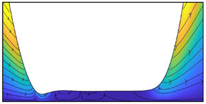
Figure 9. (a) Contours of the magnitude of the velocity,  $\sqrt {u(x,y)^{2}+v(x,y)^{2}}$ and flow streamlines with respect to a fixed reference frame in the bubble rear. (b) Effective diffusion coefficient as function of
  $Pe$ in the rear meniscus; the scale parameter is set to
  $\varepsilon =0.01$.

Figure 10. Effective velocity in the rear meniscus as a function of  $Pe$, (a) and
  $Sh_i$, (b). (c) Effective mass-transport coefficient in the rear meniscus as a function of
  $Sh_w$; the evolution of
  $Sh_i$ is not shown since there is no discernible difference in plotting
  $Sh^{\star }$. In all cases the scale parameter is set to
  $\varepsilon =0.01$.
The presence of the recirculating vortices drives the evolution of the effective Sherwood number. Differently from the bubble front, where  $Sh^{\star }$ is maximal in the uniform film region, in the rear, mass transfer is locally enhanced in proximity to the minimum of the bubble profile, see figure 10(c). There, a recirculating vortex forms and tends to squeeze out the liquid from the narrow film (see the streamlines in figure 9a). The scalar is concentrated in a narrow gap in proximity to the boundaries, enhancing the mass-transfer mechanism. This effect is more pronounced as
  $Sh_w$ (or
  $Sh_i$) increases.
The fact that shape oscillations enhance mass transfer at the bubble–fluid interface is a known phenomenon for the case of unconfined bubbles (Beek & Kramers Reference Beek and Kramers1962; Angelo, Lightfoot & Howard Reference Angelo, Lightfoot and Howard1966) and this seems to be confirmed for the case of Taylor bubbles. Hayashi et al. (Reference Hayashi, Hosoda, Tryggvason and Tomiyama2014) demonstrated that fluctuations of the bubble surface area at the bubble rear account for the main contribution to the oscillation of the effective Sherwood number. The authors arrived at this conclusion after an analysis of the velocity and the concentration fields around a Taylor bubble rising in a microchannel. Our theoretical results support this evidence.
Figure 11 shows the time evolution of the averaged concentration in the bubble rear for the advection dominated regime with  $Pe=100$,
  $Sh_w=10$ and
  $Sh_i=0$. The case has been constructed solving (2.19) with initial concentration
  $\langle c \rangle (x,0)=0$ in the entire domain and
  $\langle c \rangle (0,t)=1$ at the right boundary of the domain. The concentration front is sharp at
  $t=1$, see figure 11(a), and it gets more and more diffuse at later times, see figure 11(d). As the front moves away from the uniform film region, the concentration progressively decays as an effect of the surface mass-transfer mechanism; the breakthrough curves for this case are presented in figure 12(c). The movie of this case is available as supplementary Movie 5.

Figure 11. Time evolution of the average of the concentration,  $\langle c \rangle (x,t)$, for
  $Pe=100$,
  $Sh_w=10$,
  $Sh_i=0$ and
  $\varepsilon =0.01$. Note that the quantity plotted is a one-dimensional approximation of a two-dimensional field. See online supplementary Movie 5 for a simulation of this case.

Figure 12. Breakthrough curves for the averaged concentration in the rear meniscus as a function of  $Pe$ and
  $Sh_w$; in all the cases
  $\varepsilon =0.01$. On the left of each panel the averaged concentration at different times is plotted, on the right the rear meniscus. Cases (a,c,e) are dominated by advection; in (b,d, f) advection competes with diffusion.
When the surface mass-transfer mechanism is augmented to  $Sh_w=Pe=100$, the decay of the solute is more intense and the concentration front cannot escape the film region, figure 12(e). On the other hand, if mass transfer is turned off,
  $Sh_w=0$, the front advances towards the bubble rear almost undisturbed, figure 12(a).
When diffusion and advection compete for  $Pe=1$, the front is rapidly diffused and, as
  $Sh_w$ increases, the concentration decay in the film region becomes more intense. The effect of the Sherwood number is presented in figure 12(b,d, f). In this regime, when
  $Pe\sim Sh_w$, the solute is consumed before exiting the uniform film region, figure 12( f).
3.3. The concentration field in the uniform film
In this section, we study the mechanisms that govern the transport problem in the uniform film region, i.e. where  $\eta =1$ and
  ${\rm d}\eta /{{\rm d} x}=0$ in figure 1. In this region, the fluid is at rest since the curvature is infinite and consequently
  ${\rm d}p/{{\rm d} x}=0$, see (A6). The advection–diffusion–mass-transfer equation (2.19) reduces to
 \begin{equation} \frac{\partial \langle c \rangle }{\partial t } - \frac{\partial \langle c \rangle}{\partial x } + \frac{Sh_f^{{\star}}}{Pe} \langle c \rangle= \frac{1}{Pe} \frac{\partial^{2} \langle c \rangle}{\partial x^{2}}, \end{equation}
where
 \begin{equation} Sh^{{\star}}_f={Sh_w+Sh_i} + \dfrac{\varepsilon^{2} }{3}(Sh_w\, Sh_i-Sh_w^{2}-Sh_i^{2}). \end{equation}
Differently from the general case, the effective velocity is identically zero,  $u^{\star }_f= 0$, and the effective diffusion coefficient is equal to unity,
  $D^{\star }_f= 1$. The concentration distribution is controlled by the competition between diffusion and superficial mass transfer, while the advection term in (3.2) is there only because we consider a reference frame attached to the bubble. In the film, the effective Sherwood number
  $Sh_f^{\star }$ does not depend on the bubble geometry and, therefore, it is representative of the total mass transfer.
The main advantage in studying the transport problem in the uniform film region is that (3.2) admits analytical solutions. In fact, the desired solution can be constructed from the following Green function (i.e. the solution to a point-source initial condition centred at  $x=0$):
 \begin{equation} \mathcal{G}(x,t)=\dfrac{\exp\left(-\dfrac{Sh^{{\star}}_f}{Pe}t\right)}{\sqrt{4 {\rm \pi}t /Pe}}\exp \left( -\dfrac{(x-t)^{2}}{4t/Pe}\right). \end{equation}
Since the Green function is general and it is applicable to different sets of initial and boundary conditions, we focus on the study of a simplified case. We solve (3.2) initialising the concentration film with a pulse of height equal to unity, centred at  $x=0$, in a regime where advection dominates over diffusion,
  $Pe=100$, and competes with superficial mass transfer,
  $Sh_f^{\star }=100$. The solution is a Gaussian function that diffuses and decays in time while being advected along
  $x$, as shown in figure 13(a). Interestingly, the total mass, i.e.
 \begin{equation} \int_{-\infty}^{\infty }\mathcal{G}(x,t) \,{{\rm d} x} =\exp\left(-\dfrac{Sh_f^{{\star}}}{Pe}t\right), \end{equation}
exponentially decays, controlled by the competition between  $Sh_f^{\star }$ and
  $Pe$. Specifically, when
  $Sh_f^{\star } /Pe\rightarrow 0$, axial diffusion has an effect only on the concentration maximum, but the total mass remains constant. When
  $Sh_f^{\star } /Pe$ is finite, instead, the total mass diminishes, as shown in figure 13(b) and the residence time of the solute in the uniform film gets progressively shorter (it scales as
  $Pe/Sh_f$).

Figure 13. (a) Evolution of the averaged concentration in response to a pulse of height equal to unity, centred at  $x=0$. (b) Decay of the total mass as a function of time and the ratio
  $Sh_f^{\star }/Pe$.
The analytical solution of the transport problem in the uniform film can be employed in the construction of mechanistic or more sophisticated models where knowing the spatial and time evolution of the concentration field is of interest.
4. Conclusions
In this paper, we studied the transport of a passive scalar around a confined Taylor bubble in the presence of surface mass transfer. We derived a one-dimensional advection–diffusion–mass-transfer equation that applies to the front and rear menisci of the bubble. Specifically, advection, diffusion and superficial mass-transfer mechanisms are described through an effective velocity, effective diffusion and effective mass-transfer coefficients, expressed analytically as a function of the Pèclet and Sherwood numbers, and the film thickness. Our analysis helped in quantifying the contributions that shear flow in the film, changes in the meniscus shape and the presence of mass transfer at the domain boundaries make to the effective coefficients.
Concerning the bubble front, shear flow in the film acts to smear out the concentration distribution in the axial direction, enhancing the effective diffusion coefficient at sufficiently large Pèclet number. Interestingly, the diffusion coefficient scales with the square of the film Pèclet number, recovering the same scaling law typical of the of Aris–Taylor dispersion. Superficial mass transfer is maximum in the uniform film region, where the fluid is at rest and the solute is rapidly consumed. Also, there exist regimes where the solute is entirely consumed even before reaching the uniform film region and, when the Pèclet number balances with the Sherwood number, there exists the condition that leads to the formation of hot spots of concentration around the nose of the bubble.
The analysis of the transport problem in the bubble rear reveals that the mass transfer is locally enhanced in correspondence with the typical meniscus oscillations. There, the presence of recirculating vortices enhances the solute availability for superficial mass transfer. The analysis of the uniform film region is facilitated since the analytical solution can be obtained starting from Green functions of the presented advection–diffusion–mass-transfer equation.
Despite the fact that the motivation of our work is oriented to microfluidics applications that involve solute transport and mass transfer, its ramifications are relevant also in scenarios where the presence of a solute affects the surface tension (i.e. Marangoni effect) or even drives the flow (i.e. diffusioosmosis). In fact, cases where the gradient in the concentration of colloidal particles spontaneously drives the flow are typical of emerging fields, such as micro-filtration and bio-medical engineering: an understanding of those coupling mechanisms in the surroundings of elongated bubbles could be of help for the design of such applications. Thanks to the similar mathematical structure, the results obtained may also offer a new interpretation of heat transfer in the proximity of the Taylor bubble. More generally, several practical problems that involve thin films share a lot of similarities from a fluid mechanics perspectives (Stone Reference Stone2010), and, therefore, the proposed model may serve as a starting step to generalise the well-known Landau–Levich–Derjaguin–Bretherton problem in the presence of an active scalar.
Supplementary movies
Supplementary movies are available at https://doi.org/10.1017/jfm.2022.829.
Acknowledgements
We a thank the anonymous reviewers for their careful reading of our manuscript and their many insightful comments and suggestions.
Declaration of interests
The authors report no conflict of interest.
Appendix A. Velocity profiles in the film region
According to Bretherton (Reference Bretherton1961), the flow in the film region is expressed using a lubrication approximation. Specifically, the velocity in the axial direction is a free-surface velocity profile given by
 \begin{equation} \hat{u}(\hat{x},\hat{y})=\frac{{{\rm d}\hat{p}}}{{{\rm d}\hat{x}}} \frac{( \hat{y}^{2} - 2\hat{h} \hat{y})}{{2\mu}}. \end{equation}
The velocity in the transverse direction can be obtained starting from the continuity equation
 \begin{equation} \frac{\partial \hat{u}}{\partial \hat{x}}+\frac{\partial \hat{v}}{\partial \hat{y}}=0, \end{equation}
and integrating over the film
 \begin{equation} \hat{v}(\hat{x},\hat{y})={-}\int_0^{\hat{y}} \frac{\partial \hat{u}}{\partial \hat{x}}\,{\rm d}\hat{y}={-}\frac{1}{2\mu}\left[ \frac{{{\rm d}^{2}\hat{p}}}{{{\rm d}\hat{x}^{2}}} \left( \frac{\hat{y}^{3}}{3}-\hat{h}\hat{y}^{2}\right) - \frac{{{\rm d}\hat{p}}}{{{\rm d}\hat{x}}}\frac{{\rm d}\hat{h}}{{\rm d}\hat{x}}\hat{y}^{2} \right]. \end{equation}
Introducing the definitions of the dimensionless variables defined in (2.3a–c), (2.9a–f) and using  $\sigma \varepsilon ^{2}/h$ as the scale for the pressure, the dimensionless velocity profiles in the
  $x$ and
  $y$ directions read
 $$\begin{gather} u(x,y)=\frac{1}{2} \frac{{\rm d} p}{{\rm d} x}(y^{2} - 2 \eta y), \end{gather}$$
 $$\begin{gather}{v}({x},{y})={-}\frac{1}{2}\left[ \frac{{{\rm d}^{2} p }}{{{{\rm d} x} ^{2}}} \left( \frac{{y}^{3}}{3}-{\eta}{y}^{2}\right) - y^{2} \frac{{{\rm d}\eta }}{{{{\rm d} x} }} \frac{{{\rm d}p }}{{{\rm d} x}} \right]. \end{gather}$$
Expressing the pressure gradient as a function of  $\eta$ using (2.2)
 \begin{equation} \frac{{\rm d}p}{{\rm d} x}={-}\frac{{\rm d}^{3}\eta}{{{\rm d} x}^{3}}={-}\dfrac{\eta-1}{\eta^{3}}, \end{equation}
we obtain
 $$\begin{gather} u(x,y)={-} \dfrac{\eta-1}{2\eta^{3}}(y^{2} - 2 \eta y), \end{gather}$$
 $$\begin{gather}{v}({x},{y})=\frac{3-2\eta}{2\eta^{4}} \left( \frac{{y}^{3}}{3}-{\eta}{y}^{2}\right) \dfrac{{\rm d}\eta}{{\rm d} x} - y^{2} \dfrac{\eta-1}{2\eta^{3}}\dfrac{{\rm d}\eta}{{\rm d} x} . \end{gather}$$
Appendix B. Derivation of the transport equation by means of two-scale expansion
In the following sections the derivation of the effective equation for the average concentration is carried out separately for each regime, identified by the magnitude of the Pèclet number.
B.1. Advection dominated regime, $Pe={O}(\varepsilon ^{-1})$

In regimes where  $Pe={O}(\varepsilon ^{-1})$ or
  $\alpha =1$, replacing the expanded variables (2.17) and the dimensionless numbers (2.16a–c) in the equation for the concentration, (2.10), we obtain
 \begin{align} &-\varepsilon^{\alpha-2} \frac{\partial^{2} c_0}{\partial y^{2}} + \varepsilon^{0} \left[ \frac{\partial c_0}{\partial t} + (u(x,y)-1) \frac{\partial c_0}{\partial x} {+v(x,y)\frac{\partial c_0}{\partial y}}- \varepsilon^{\alpha -1}\frac{\partial^{2} c_1}{\partial y^{2}} \right]\nonumber\\ &\quad + \varepsilon \left[ \frac{\partial c_1}{\partial t} + \left(u(x,y) - 1 \right) \frac{\partial c_1}{\partial x} {+v(x,y)\frac{\partial c_1}{\partial y}}- \varepsilon^{\alpha - 1} \frac{\partial^{2} c_0}{\partial x^{2}} - \varepsilon^{\alpha - 1} \frac{\partial^{2} c_2}{\partial y^{2}}\right] + \ldots=0, \end{align}
where  $u(x,y)$ and
  $v(x,y)$ are given in (A7) and (A8), respectively. Similarly, the expanded boundary conditions, (2.12) and (2.15), yield
 $$\begin{gather} \dfrac{ \partial c_0}{\partial y}+\varepsilon \dfrac{ \partial c_1}{\partial y}+\varepsilon^{2}\dfrac{ \partial c_2}{\partial y}=\varepsilon^{2+\beta}c_0+\varepsilon^{3+\beta}c_1+\varepsilon^{4+\beta}c_2+ {O}(\varepsilon^{2}) \quad {\rm at} \ y=0, \end{gather}$$
 $$\begin{gather}-\dfrac{ \partial c_0}{\partial y}-\varepsilon \dfrac{ \partial c_1}{\partial y}-\varepsilon^{2}\dfrac{ \partial c_2}{\partial y}=\varepsilon^{2+\gamma}c_0+\varepsilon^{3+\gamma}c_1+\varepsilon^{4+\gamma}c_2+ {O}(\varepsilon^{2}) \quad {\rm at} \ y=\eta. \end{gather}$$
 Collecting the terms at the leading order  ${O}(\varepsilon ^{-1})$, we get
 \begin{equation}
\left.\begin{array}{cc@{}} - \dfrac{\partial^{2}
c_0}{\partial y^{2}} =0 & y\in [0,\eta], \\ \dfrac{
\partial c_0}{\partial y} =0 & {\rm at}\ y=0, \\ \dfrac{
\partial c_0}{\partial y}=0 & {\rm at}\ y=\eta. \end{array}
\right\} \end{equation}
\begin{equation}
\left.\begin{array}{cc@{}} - \dfrac{\partial^{2}
c_0}{\partial y^{2}} =0 & y\in [0,\eta], \\ \dfrac{
\partial c_0}{\partial y} =0 & {\rm at}\ y=0, \\ \dfrac{
\partial c_0}{\partial y}=0 & {\rm at}\ y=\eta. \end{array}
\right\} \end{equation}
The homogeneity of the equation and the boundary conditions in (B4) ensure that the boundary-value problem admits a trivial solution (i.e. that  $c_0$ is independent of
  $y$), and, therefore,
  $c_0$ is the average concentration defined in (2.18),
  $c_0(x,t)=\langle c \rangle (x,t)$. This is true as long as
  $\alpha <2$,
  $\beta >-2$ and
  $\gamma >-2$, namely,
  $Pe\ll {O}(\varepsilon ^{-2})$ and
  $Sh_w\ll {O}(\varepsilon ^{-2})$ and
  $Sh_i\ll {O}(\varepsilon ^{-2})$. At the next order,
  ${O}(1)$, we obtain the following boundary-value problem:
 \begin{equation} \left.\begin{array}{c@{}}
- \dfrac{\partial^{2} c_1}{\partial y^{2}} ={-}
\varepsilon^{1- \alpha } \dfrac{\partial c_0}{\partial t} -
\varepsilon^{1- \alpha }\left[
-\dfrac{\eta-1}{2\eta^{3}}\left( y^{2} - 2\eta y\right) - 1
\right] \dfrac{\partial c_0}{\partial
x}+v(x,y)\dfrac{\partial c_0}{\partial y}, \\
\dfrac{\partial c_1}{\partial y} = \varepsilon^{1+\beta }
c_0 \quad {\rm at} \ y=0, \\ -\dfrac{\partial c_1}{\partial
y} = \varepsilon^{1+\gamma } c_0 \quad {\rm at} \ y=\eta.
\end{array} \right\} \end{equation}
\begin{equation} \left.\begin{array}{c@{}}
- \dfrac{\partial^{2} c_1}{\partial y^{2}} ={-}
\varepsilon^{1- \alpha } \dfrac{\partial c_0}{\partial t} -
\varepsilon^{1- \alpha }\left[
-\dfrac{\eta-1}{2\eta^{3}}\left( y^{2} - 2\eta y\right) - 1
\right] \dfrac{\partial c_0}{\partial
x}+v(x,y)\dfrac{\partial c_0}{\partial y}, \\
\dfrac{\partial c_1}{\partial y} = \varepsilon^{1+\beta }
c_0 \quad {\rm at} \ y=0, \\ -\dfrac{\partial c_1}{\partial
y} = \varepsilon^{1+\gamma } c_0 \quad {\rm at} \ y=\eta.
\end{array} \right\} \end{equation}
Since  $c_0$ is independent of
  $y$, the last term on the right-hand side of (B5) vanishes, i.e.
  $\partial c_0/\partial y=0$. A necessary condition for the existence of the solution is that the integration of (B5) between
  $y=0$ and
  $y=\eta$ with the use of its boundary conditions is identically zero. This condition is known in the literature as the compatibility condition or Fredholm alternative (see e.g. Rubinstein & Mauri Reference Rubinstein and Mauri1986; Auriault Reference Auriault2002; Mikelić et al. Reference Mikelić, Devigne and van Duijn2006). Unfortunately, for the problem considered, the initial and boundary data for
  $c_0$ are incompatible and, therefore, this procedure leads to a discontinuous solution. This issue can be solved by integrating (B5) between
  $y=0$ and
  $y=\eta$ with the addition of a smaller correction, of the order of
  $\varepsilon$,
 \begin{equation} \frac{\partial c_0}{\partial t} - \left( -\dfrac{\eta-1}{3\eta} + 1\right)\frac{\partial c_0}{\partial x} +\frac{c_0\varepsilon^{\alpha} }{\eta}\left( \varepsilon^{\beta}+\varepsilon^{\gamma}\right) ={O}(\varepsilon) . \end{equation}
A similar procedure has been employed in Mikelić et al. (Reference Mikelić, Devigne and van Duijn2006) and Rubinstein & Mauri (Reference Rubinstein and Mauri1986). By inspection of (B6) we get an additional constraint on the Pèclet and the Sherwood numbers, i.e.  $\alpha +\beta >-1$ and
  $\alpha +\gamma >-1$ (
  $Sh_w/Pe\ll {O}(\varepsilon ^{-1})$ and
  $Sh_i/Pe\ll {O}(\varepsilon ^{-1})$).
Substituting (B6) into (B5), we obtain a boundary-value problem for the computation of  $c_1(x,y,t)$
 \begin{equation} \left.\begin{array}{c@{}}
- \dfrac{\partial^{2} c_1}{\partial y^{2}} =
\varepsilon^{\alpha-1} \dfrac{\eta-1}{2\eta^{3}}\left(
y^{2}-2\eta y +\dfrac{2}{3}\eta^{2} \right)\dfrac{\partial
c_0}{\partial x} + \varepsilon
\dfrac{c_0}{\eta}\left(\varepsilon^{\beta}+\varepsilon^{\gamma}\right),
\\ \dfrac{\partial c_1}{\partial y} = \varepsilon^{1+\beta
} c_0 \quad {\rm at} \ y=0, \\ -\dfrac{\partial
c_1}{\partial y} = \varepsilon^{1+\gamma } c_0 \quad {\rm
at} \ y=\eta, \end{array} \right\}
\end{equation}
\begin{equation} \left.\begin{array}{c@{}}
- \dfrac{\partial^{2} c_1}{\partial y^{2}} =
\varepsilon^{\alpha-1} \dfrac{\eta-1}{2\eta^{3}}\left(
y^{2}-2\eta y +\dfrac{2}{3}\eta^{2} \right)\dfrac{\partial
c_0}{\partial x} + \varepsilon
\dfrac{c_0}{\eta}\left(\varepsilon^{\beta}+\varepsilon^{\gamma}\right),
\\ \dfrac{\partial c_1}{\partial y} = \varepsilon^{1+\beta
} c_0 \quad {\rm at} \ y=0, \\ -\dfrac{\partial
c_1}{\partial y} = \varepsilon^{1+\gamma } c_0 \quad {\rm
at} \ y=\eta, \end{array} \right\}
\end{equation}
whose integration leads to
 \begin{align} c_1(x,y,t) &={-}\varepsilon^{1-\alpha} \dfrac{\eta-1}{2\eta^{3}}\left( \frac{y^{4}}{12} - \frac{\eta y^{3}}{3} +\frac{\eta^{2}y^{2}}{3} \right)\frac{\partial c_0}{\partial x} + \varepsilon \left[ \varepsilon^{\beta}\left( y-\frac{y^{2}}{2\eta}\right)-\varepsilon^{\gamma} \frac{y^{2}}{2 \eta} \right] c_0\nonumber\\ &\quad+ C_0(x,t), \end{align}
where  $C_0(x,t)$ is an arbitrary function. To determine
  $C_0(x,t)$, we impose that
  $c_1$ has zero average, namely
  $\int _0^{\eta } c_1\, {{\rm d} y} =0$, giving
 \begin{equation} C_0(x,t)= \varepsilon^{1-\alpha} \dfrac{{(\eta-1)}\eta}{45} \frac{\partial c_0}{\partial x}- \varepsilon \eta \left( \frac{\varepsilon^{\beta}}{3}-\frac{\varepsilon^{\gamma}}{6}\right) c_0. \end{equation}
Combining (B8) and (B9) we get the final expression for  $c_1(x,y,t)$
 \begin{align} c_1 &={-}\varepsilon^{1-\alpha} \dfrac{(\eta-1)}{2\eta^{3}}\left( \frac{y^{4}}{12} - \frac{\eta y^{3}}{3} +\frac{\eta^{2}y^{2}}{3}-\frac{2\eta^{4}}{45} \right)\frac{\partial c_0}{\partial x} \nonumber\\ &\quad + \varepsilon \left[ \varepsilon^{\beta}\left( y-\frac{y^{2}}{2\eta}-\frac{\eta}{3} \right)+\varepsilon^{\gamma}\left( \frac{\eta}{6}-\frac{y^{2}}{2 \eta}\right) \right]c_0. \end{align}
 Then, we collect the terms of order  ${O}(\varepsilon )$ in (B1), including the additional terms resulting from (B6), and we obtain a boundary-value problem for
  $c_2(x,y,t)$
 \begin{equation} \left.\begin{array}{c@{}}
-\dfrac{\partial^{2} c_2}{\partial y^{2}} ={-}
\varepsilon^{1-\alpha}\left( u(x,y)-
1\right)\dfrac{\partial c_1}{\partial x} +
\dfrac{\partial^{2} c_0}{\partial x^{2}} -
\varepsilon^{1-\alpha} \dfrac{\partial c_1}{\partial t} -
\varepsilon^{1-\alpha}v(x,y) \dfrac{\partial c_1}{\partial
y}\\ \quad \ \, - \varepsilon^{-\alpha} \left[
\dfrac{\partial c_0}{\partial t} - \left(
-\dfrac{\eta-1}{3\eta} + 1\right)\dfrac{\partial
c_0}{\partial x} +\varepsilon^{\alpha}
\dfrac{c_0}{\eta}\left(
\varepsilon^{\beta}+\varepsilon^{\gamma}\right)\right],\\
\dfrac{\partial c_2}{\partial y} =
\varepsilon^{1+\beta}c_1\quad {\rm at} \ y=0, \\
-\dfrac{\partial c_2}{\partial y} =
\varepsilon^{1+\gamma}c_1\quad {\rm at} \ y=\eta.
\end{array} \right\} \end{equation}
\begin{equation} \left.\begin{array}{c@{}}
-\dfrac{\partial^{2} c_2}{\partial y^{2}} ={-}
\varepsilon^{1-\alpha}\left( u(x,y)-
1\right)\dfrac{\partial c_1}{\partial x} +
\dfrac{\partial^{2} c_0}{\partial x^{2}} -
\varepsilon^{1-\alpha} \dfrac{\partial c_1}{\partial t} -
\varepsilon^{1-\alpha}v(x,y) \dfrac{\partial c_1}{\partial
y}\\ \quad \ \, - \varepsilon^{-\alpha} \left[
\dfrac{\partial c_0}{\partial t} - \left(
-\dfrac{\eta-1}{3\eta} + 1\right)\dfrac{\partial
c_0}{\partial x} +\varepsilon^{\alpha}
\dfrac{c_0}{\eta}\left(
\varepsilon^{\beta}+\varepsilon^{\gamma}\right)\right],\\
\dfrac{\partial c_2}{\partial y} =
\varepsilon^{1+\beta}c_1\quad {\rm at} \ y=0, \\
-\dfrac{\partial c_2}{\partial y} =
\varepsilon^{1+\gamma}c_1\quad {\rm at} \ y=\eta.
\end{array} \right\} \end{equation}
Integrating (B11) between  $y=0$ and
  $y=\eta$ with the use of (A7) and (A8) we get
 \begin{align} &-\left.\dfrac{\partial c_2}{\partial y}\right|_{y=\eta}+\left.\dfrac{\partial c_2}{\partial y}\right|_{y=0}\nonumber\\ &\quad ={-} \varepsilon^{1-\alpha}\int_0^{\eta}\left[ -\dfrac{\eta-1}{2\eta^{3}}(y^{2}- 2\eta y)- 1\right]\dfrac{\partial c_1}{\partial x}{{\rm d} y} + \int_0^{\eta}\dfrac{\partial^{2} c_0}{\partial x^{2}}\,{{\rm d} y}\nonumber\\ &\qquad - \varepsilon^{1-\alpha}\int_0^{\eta} \dfrac{\partial c_1}{\partial t}{{\rm d} y} - \varepsilon^{1-\alpha}\int_0^{\eta}\dfrac{1}{2}\left[ \dfrac{3-2\eta}{\eta^{4}}\dfrac{{\rm d}\eta}{{\rm d} x} \left( \dfrac{{y}^{3}}{3}-{\eta}{y}^{2}\right) - y^{2} \dfrac{\eta-1}{\eta^{3}}\dfrac{{\rm d}\eta}{{\rm d} x} \right] \dfrac{\partial c_1}{\partial y}\,{{\rm d} y}\nonumber\\ &\qquad - \varepsilon^{-\alpha}\int_0^{\eta} \left[ \dfrac{\partial c_0}{\partial t} - \left( -\dfrac{\eta-1}{3\eta} + 1\right)\dfrac{\partial c_0}{\partial x} +\varepsilon^{\alpha} \dfrac{c_0}{\eta}\left( \varepsilon^{\beta}+\varepsilon^{\gamma}\right)\right]{{\rm d} y}. \end{align}
The integrals in (B12) are carried out recalling that  $c_0(x,t)$ is independent of
  $y$, using the full expression of
  $c_1(x,y,t)$ given in (B10), and the relation
 \begin{equation} \int_0^{\eta(x)} \dfrac{\partial c_1}{\partial t}{{\rm d} y}=\dfrac{\partial }{\partial t}\int_0^{\eta(x)} c_1\,{\rm d}y=0, \end{equation}
since  $\eta (x)$ does not depend upon time and
  $c_1(x,y,t)$ has zero average. Using the boundary conditions from (B11) to replace the left-hand side of (B12), we get the following conservation equation for the leading-order
  $c_0$ (or the averaged concentration):
 \begin{align} &\frac{\partial c_0}{\partial t} + \left[ \frac{\eta-1}{3\eta}-\varepsilon^{2-\alpha}\frac{(73\eta-8)(\eta-1)}{3780\eta}\dfrac{{\rm d}\eta}{{\rm d} x} - \varepsilon^{2+\gamma}\dfrac{14\eta(\eta-1)+(73\eta+47)\,{\rm d}\eta/{{\rm d} x}}{360\eta}\right.\nonumber\\ &\qquad \left. +\, \varepsilon^{2+\beta}\dfrac{16\eta(\eta-1)+(47\eta+13)\,{\rm d}\eta/{{\rm d} x}}{360\eta}- 1 \right]\frac{\partial c_0}{\partial x} \nonumber\\ &\qquad +\left[\varepsilon^{\alpha}\frac{\varepsilon^{\beta}+\varepsilon^{\gamma}}{\eta} + \dfrac{\varepsilon^{2+\alpha}}{3} ({\varepsilon^{\beta+\gamma}}-{\varepsilon^{2\beta}-\varepsilon^{2\gamma}} ) \right.\nonumber\\ &\qquad \left.-\left(\dfrac{\varepsilon^{2+\gamma}(7\eta-18)+\varepsilon^{2+\beta}(7-3\eta)}{120 \eta}\right) \dfrac{{\rm d}\eta}{{\rm d} x} \right]c_0\nonumber\\ &\quad=\varepsilon^{\alpha} \left[ 1+\varepsilon^{2-2\alpha}\frac{2(\eta-1)^{2}}{945} \right] \frac{\partial^{2} c_0}{\partial x^{2}}. \end{align}
Advection, superficial mass transfer and diffusion are accounted for through effective coefficients. In this regime, transverse advection affects both the effective advection and the effective mass-transfer terms, while the effective diffusion is driven by the flow in the axial direction only. Equation (B14) represents the generalisation of the Aris–Taylor dispersion to the film region of a Taylor bubble.
Note that the effective equation (B14) converges to the results obtained by Mikelić et al. (Reference Mikelić, Devigne and van Duijn2006) when (i) advection balances with interfacial mass transfer at the wall  ${O}(Pe)= {O}(Sh_w)={O}(\varepsilon ^{-1})$ (or
  $\beta +\alpha =0$ with
  $\alpha =1$); (ii) mass transfer at the interface is negligible; (iii) the interface is flat like in the case of a straight channel (
 $\eta =1$) and we use back (A6) to restore the
  ${\rm d}p/{{\rm d} x}$ term; (iv) we look at the problem in a fixed reference frame. Also, if both mass-transfer mechanisms are turned off, we recover the classical Aris–Taylor dispersion equation (Taylor Reference Taylor1953; Aris Reference Aris1956).
For the sake of completeness, the second-order correction  $c_2$ can be determined by solving (B11) and choosing that
  $\int _0^{\eta } c_2 \,{{\rm d} y} =0$. We do not report here the final expression since we are primarily interested in the evolution of the averaged concentration. As is shown in Appendix D, the first-order correction is negligible within the region of applicability of the model.
B.2. Competition between advection and diffusion, $Pe={O}({1})$

In regimes where advection competes with diffusion for  $Pe={O}(1)$ or
  $\alpha =0$, the expanded equation yields
 \begin{align} &-\varepsilon^{\alpha-2} \frac{\partial^{2} c_0}{\partial y^{2}} - \varepsilon^{\alpha -1}\frac{\partial^{2} c_1}{\partial y^{2}}+ \frac{\partial c_0}{\partial t} + (u(x,y)-1) \frac{\partial c_0}{\partial x} {+v(x,y)\frac{\partial c_0}{\partial y}} - \varepsilon^{\alpha} \frac{\partial^{2} c_2}{\partial y^{2}}\nonumber\\ &\quad - \varepsilon^{\alpha} \frac{\partial^{2} c_0}{\partial x^{2}} + \ldots=0. \end{align}
Collecting the terms at the leading orders,  ${O}(\varepsilon ^{-2})$ and
  ${O}(\varepsilon ^{-1})$, in (B15) and (B2) we get following boundary-value problems:
 \begin{equation}
\left.\begin{array}{cc@{}} - \dfrac{\partial^{2}
c_0}{\partial y^{2}} =0 & y\in [0,\eta], \\ \dfrac{
\partial c_0}{\partial y} =0 & {\rm at}\ y=0, \\ \dfrac{
\partial c_0}{\partial y}=0 & {\rm at}\ y=\eta,
\end{array}\right\}\quad \left.\begin{array}{cc@{}} -
\dfrac{\partial^{2} c_1}{\partial y^{2}} =0 & y\in
[0,\eta], \\ \dfrac{ \partial c_1}{\partial y} =0 & {\rm
at}\ y=0, \\ \dfrac{ \partial c_1}{\partial y}=0 & {\rm
at}\ y=\eta, \end{array}
\right\}
\end{equation}
\begin{equation}
\left.\begin{array}{cc@{}} - \dfrac{\partial^{2}
c_0}{\partial y^{2}} =0 & y\in [0,\eta], \\ \dfrac{
\partial c_0}{\partial y} =0 & {\rm at}\ y=0, \\ \dfrac{
\partial c_0}{\partial y}=0 & {\rm at}\ y=\eta,
\end{array}\right\}\quad \left.\begin{array}{cc@{}} -
\dfrac{\partial^{2} c_1}{\partial y^{2}} =0 & y\in
[0,\eta], \\ \dfrac{ \partial c_1}{\partial y} =0 & {\rm
at}\ y=0, \\ \dfrac{ \partial c_1}{\partial y}=0 & {\rm
at}\ y=\eta, \end{array}
\right\}
\end{equation}
that ensure that both  $c_0(x,t)$ and
  $c_1(x,t)$ are independent of
  $y$. This is true as long as
  $\beta \geqslant 0$ and
  $\gamma \geqslant 0$. At the next order,
  ${O}(1)$, we obtain
 \begin{equation} \left.\begin{array}{c@{}}
- \dfrac{\partial^{2} c_2}{\partial y^{2}} ={-}
\varepsilon^{- \alpha }\left[\dfrac{\partial c_0}{\partial
t} + (u(x,y)-1) \dfrac{\partial c_0}{\partial x}{+}v(x,y)
\dfrac{\partial c_0}{\partial y}\right] +
\dfrac{\partial^{2} c_0}{\partial x^{2}}, \\
\dfrac{\partial c_2}{\partial y} = \varepsilon^{1+\beta }
c_0 \quad {\rm at} \ y=0, \\ -\dfrac{\partial c_2}{\partial
y} = \varepsilon^{1+\gamma } c_0 \quad {\rm at} \ y=\eta.
\end{array} \right\} \end{equation}
\begin{equation} \left.\begin{array}{c@{}}
- \dfrac{\partial^{2} c_2}{\partial y^{2}} ={-}
\varepsilon^{- \alpha }\left[\dfrac{\partial c_0}{\partial
t} + (u(x,y)-1) \dfrac{\partial c_0}{\partial x}{+}v(x,y)
\dfrac{\partial c_0}{\partial y}\right] +
\dfrac{\partial^{2} c_0}{\partial x^{2}}, \\
\dfrac{\partial c_2}{\partial y} = \varepsilon^{1+\beta }
c_0 \quad {\rm at} \ y=0, \\ -\dfrac{\partial c_2}{\partial
y} = \varepsilon^{1+\gamma } c_0 \quad {\rm at} \ y=\eta.
\end{array} \right\} \end{equation}
Integrating (B17) between  $y = 0$ and
  $y = \eta$ we obtain
 \begin{align} -\left. \dfrac{\partial c_2}{\partial y}\right|_{y=\eta}+\left. \dfrac{\partial c_2}{\partial y}\right|_{y=0}& ={-} \varepsilon^{- \alpha }\left[ \int_0^{\eta}\dfrac{\partial c_0}{\partial t}\,{{\rm d} y} + \int_0^{\eta}(u(x,y)-1) \dfrac{\partial c_0}{\partial x}\,{{\rm d} y} \right.\nonumber\\ &\quad \left.+\int_0^{\eta} v(x,y) \dfrac{\partial c_0}{\partial y}\,{{\rm d} y}\right] + \int_0^{\eta} \dfrac{\partial^{2} c_0}{\partial x^{2}}\,{{\rm d} y}. \end{align}
Using the boundary conditions to replace the left-hand side of (B18), the full expression of  $u(x,y)$ given in (A7) and recalling that
  $c_0(x,t)$ is independent of
  $y$, we get the following conservation equation for the averaged concentration:
 \begin{equation} \frac{\partial c_0}{\partial t} + \left( \frac{\eta-1}{3\eta}- 1 \right)\frac{\partial c_0}{\partial x} +\varepsilon^{\alpha}\frac{\varepsilon^{\beta}+\varepsilon^{\gamma}}{\eta} c_0 = \varepsilon^{\alpha} \frac{\partial^{2} c_0}{\partial x^{2}}. \end{equation}
In this regime, the contribution of the transverse advection vanishes since  $\partial c_0/\partial y=0$ in (B18) and the diffusive term is limited to molecular diffusion only.
By inspection of (B14) and (B19) we can observe that the solution obtained previously for the advection dominated regime embeds the solution obtained in this section for regimes where advection and diffusion compete. Specifically, when  $\alpha =1$, several terms in (B14) become small and (B14) reduces to (B19).
B.3. Diffusion dominated regime, $Pe={O}({\varepsilon })$ or smaller

When the Pèclet number is small,  $Pe={O}({\varepsilon })$ or smaller, diffusion dominates over advection and the relevant time scale is the diffusive time scale instead of the advective one used in (2.9a–f). In this case, the same procedure described in previous sections can be applied, provided that the time variable in (2.10) is rescaled as follows:
 \begin{equation} \frac{\partial c}{\partial t} \rightarrow \varepsilon^{\alpha} \frac{\partial c}{\partial t_d}, \end{equation}
where  $t_d=\hat {t}/\tau _d$ is the dimensionless diffusion time. Plugging the rescaled time variable into (2.10), after doing the expansions, we get the following cascade of equations:
 \begin{equation} -\varepsilon^{\alpha-2} \frac{\partial^{2} c_0}{\partial y^{2}} - \varepsilon^{\alpha -1}\frac{\partial^{2} c_1}{\partial y^{2}}+ \varepsilon^{\alpha}\left( \frac{\partial c_0}{\partial t_d} - \frac{\partial^{2} c_2}{\partial y^{2}} - \frac{\partial^{2} c_0}{\partial x^{2}} \right) + \ldots=0, \end{equation}
coupled with the boundary conditions (B2). It is straightforward to show that this procedure leads to the following diffusion–mass-transfer equation:
 \begin{equation} \frac{\partial c_0}{\partial t_d} +\frac{\varepsilon^{\beta}+\varepsilon^{\gamma}}{\eta} c_0 = \frac{\partial^{2} c_0}{\partial x^{2}}, \end{equation}
provided that  $\alpha \leqslant -1$,
  $\alpha +\beta =0$ and
  $\alpha +\gamma =0$. In this regime, the effect of advection (in both directions) is negligible. If we switch back to the advective time, (B22) is identical to (B19) once we drop the advective term
 \begin{equation} \frac{\partial c_0}{\partial t}+ \varepsilon^{\alpha}\frac{\varepsilon^{\beta}+\varepsilon^{\gamma}}{\eta} c_0 = \varepsilon^{\alpha} \frac{\partial^{2} c_0}{\partial x^{2}}. \end{equation}
Therefore, the effective advection–diffusion–mass-transfer equation (B14) embeds all three regimes considered.
Appendix C. Further analysis of the effective velocity and the effective Sherwood number
In this section, we study the relative importance of the different terms appearing in the effective velocity (2.20) and the effective Sherwood number (2.21). If we define
 \begin{equation} \left.\begin{gathered} \mathcal{I}_1= \frac{\eta-1}{3\eta}, \quad \mathcal{I}_2={-}\varepsilon^{2}Pe\,\frac{(73\eta-8)(\eta-1)}{3780\eta}\dfrac{{\rm d}\eta}{{\rm d} x},\\ \mathcal{I}_3= \varepsilon^{2}\left[Sh_i\dfrac{14\eta(\eta-1)+(73\eta+47) \,{\rm d}\eta/{{\rm d} x}}{360\eta}-Sh_w\dfrac{16\eta(\eta-1)+(47\eta+13)\, {\rm d}\eta/{{\rm d} x}}{360\eta}\right], \\ \mathcal{M}_1=\frac{Sh_w+Sh_i}{\eta}, \quad \mathcal{M}_2= \dfrac{\varepsilon^{2} }{3}(Sh_w\, Sh_i-Sh_w^{2}-Sh_i^{2} ),\\ \mathcal{M}_3={-}\varepsilon^{2}Pe\dfrac{Sh_i(7\eta-18)+Sh_w(7-3\eta)}{120 \eta} \dfrac{{\rm d}\eta}{{\rm d} x}, \end{gathered}\right\} \end{equation}
we can compute the relative importance of the different terms with respect to the dominant one, i.e.  $\mathcal {I}_2/\mathcal {I}_1$ and
  $\mathcal {I}_3/\mathcal {I}_1$ for
  $u^{\star }$, and
  $\mathcal {M}_2/\mathcal {M}_1$ and
  $\mathcal {M}_3/\mathcal {M}_1$ for
  $Sh^{\star }$, respectively. We plot such ratios referring to the most general case where
  $Pe=Sh_w=Sh_i={O}(\varepsilon ^{-1})$ (regime I) in figure 14(a). Clearly, the terms
  $\mathcal {I}_2$ and
  $\mathcal {I}_3$ (which represent the contribution of transverse velocity and superficial mass transfer to the overall effective advection) are negligible compared with
  $\mathcal {I}_1$ (which represents the contribution of axial velocity only). This is true also in the bubble rear; the spikes in figure 14(b) originate from division by zero when
  $\eta =1$, but, at such points,
  $u^{\star }\approx 0$. Similarly, the terms
  $\mathcal {M}_2$ and
  $\mathcal {M}_3$ are much smaller with respect to
  $\mathcal {M}_1$ in both the front and rear menisci.


From the practical point of view, in the region of validity of the model (see § 2.4), we can approximate the effective coefficients as
 \begin{equation} u^{{\star}}\approx\frac{\eta-1}{3\eta} \quad Sh^{{\star}}\approx\frac{Sh_w+Sh_i}{\eta}. \end{equation}
Appendix D. First-order corrections of the concentration field
In § 3.1 we focused on the time evolution of the averaged concentration, that is, in the asymptotic expansion (2.17), the zeroth-order term. For the sake of completeness, we study the concentration field including corrections up to the first order, i.e.  $c(x,y,t)=c_0(x,t)+\varepsilon c_1(x,y,t)$. Once
  $c_0(x,t)$ is known by solving (2.19), the first-order term
  $\varepsilon c_1(x,y,t)$ can be computed directly from (B10).
To prove that, within the region of applicability of the model (see figure 2) the first-order correction is small, we analyse the order of magnitude of the correction, estimated as
 \begin{equation} {O}(\varepsilon
c_1)={O}(\varepsilon^{2} Pe\, \eta^{2})
\frac{\partial c_0}{\partial x} + {O}(\varepsilon^{2}(Sh_w+Sh_i)\eta) c_0.
\end{equation}
\begin{equation} {O}(\varepsilon
c_1)={O}(\varepsilon^{2} Pe\, \eta^{2})
\frac{\partial c_0}{\partial x} + {O}(\varepsilon^{2}(Sh_w+Sh_i)\eta) c_0.
\end{equation}
The axial derivative term in (D1) is controlled by the competition between the Pèclet number and the bubble shape, while the second term vanishes only when surface mass transfer is absent or negligible. When  $Pe$ is equal to or smaller than
  ${O}(\varepsilon ^{-1})$, the axial derivative term does not exceed
  ${O}( \varepsilon \eta ^{2})$. Similarly, when
  $Sh_w$ or
  $Sh_i$ is smaller than or equal to
  ${O}(\varepsilon ^{-1})$, the second term does not exceed
  ${O}( \varepsilon \eta )$. Therefore, for all the regimes classified in § 2.5, it is reasonable to neglect high-order terms and to look only at the evolution of the averaged concentration.
Figure 15 shows the time evolution of  $\varepsilon c_1(x,y,t)$ for the same case depicted in figure 5 corresponding to regime I in figure 2. At early times, the correction is around 10 % only in the proximity of the concentration front, but it becomes negligible when the front has been diffused. As expected, the axial derivative of
  $c_0$ contributes only in proximity to sharp variations of the concentration field.

Figure 15. Time evolution of the first-order correction term  $\varepsilon c_1(x,y,t)$ in the expansion (2.17) for regime I, i.e.
  $Pe=100$,
  $Sh_w=100$,
  $Sh_i=0$ and
  $\varepsilon =0.01$. See also online supplementary Movie 4 for a simulation of this case.
The scenario changes dramatically when the model is brought closer to or out of its validity range. If  $Pe={O}(\varepsilon ^{-2})$, the axial derivative term becomes at least of order one; the same happens for the second term if the Sherwood numbers are of order
  $\varepsilon ^{-2}$. Although the model is not strictly applicable under such conditions, using the model closer to or outside of its theoretical limits would require consideration of higher-order corrections instead of the zeroth-order dynamics only.


 Open access