


1. Introduction
An important problem in the study of turbulent flows is to estimate the functional dependence of global properties (such as energy dissipation, drag force, heat and mass transport, and mixing efficiency) on input parameters. The lack of analytical solutions of the Navier–Stokes equations in the fully turbulent regime has forced the scientific community to adopt a multi-faceted approach to this problem, in which simple physical theories and reduced models are proposed, and then corroborated by direct numerical simulations (DNS) and/or results from laboratory experiments. However, the inability to perform simulations and experiments in the extreme parameter regimes that often concern atmospheric, oceanic and astrophysical flows and engineering applications leaves these theories unsubstantiated.
In these extreme parameter regimes, an alternative approach that can provide meaningful information is to obtain rigorous bounds on the aforementioned global properties. The first method to obtain bounds was developed by Howard (Reference Howard1963) and Busse (Reference Busse1969), but it was not until the 1990s that bounding techniques gained general popularity, with the introduction of the so-called ‘background method’ by Doering and Constantin (Doering & Constantin Reference Doering and Constantin1992, Reference Doering and Constantin1994, Reference Doering and Constantin1996; Constantin & Doering Reference Constantin and Doering1995). The background method is based on ideas from Hopf to produce a priori estimates for the solutions of the Navier–Stokes equations with inhomogeneous boundary conditions (Hopf Reference Hopf1955). So far, it has been applied to many different fluid mechanics problems (Doering & Constantin Reference Doering and Constantin1992, Reference Doering and Constantin1996; Constantin & Doering Reference Constantin and Doering1995; Caulfield & Kerswell Reference Caulfield and Kerswell2001; Tang, Caulfield & Young Reference Tang, Caulfield and Young2004; Whitehead & Doering Reference Whitehead and Doering2011; Goluskin & Doering Reference Goluskin and Doering2016; Fantuzzi Reference Fantuzzi2018; Fantuzzi, Pershin & Wynn Reference Fantuzzi, Pershin and Wynn2018; Kumar & Garaud Reference Kumar and Garaud2020; Arslan et al. Reference Arslan, Fantuzzi, Craske and Wynn2021a,Reference Arslan, Fantuzzi, Craske and Wynnb; Fan, Jolly & Pakzad Reference Fan, Jolly and Pakzad2021; Kumar et al. Reference Kumar, Arslan, Fantuzzi, Craske and Wynn2022). See Fantuzzi, Arslan & Wynn (Reference Fantuzzi, Arslan and Wynn2022) for a recent review.
In the background method, we write the total flow field as a sum of two flow fields: the background flow and the perturbed flow. To obtain a bound on the desired bulk quantity requires choosing a background field that satisfies a certain integral constraint (extracted from the governing equations of the perturbed flow). Generally, one takes one of the following two routes. The first route is to specify a functional form of the background flow and then use standard inequalities. This route leads to an analytical but suboptimal bound on the bulk quantity as a function of system parameters. The second route is to find the best possible bound (optimal bound) through a variational formulation of the background method in which one solves the corresponding Euler–Lagrange equations, usually numerically. Numerous studies pertaining to the background flow have concentrated on the scaling of optimal bounds as a function of the principal flow parameter, such as the Reynolds number and the Rayleigh number. However, only a handful of them studied the variation of these bounds with the shape of the domain. One such study is by Wen et al. (Reference Wen, Chini, Dianati and Doering2013), where the authors were interested in determining the dependence on aspect ratio of the optimal bound on heat transfer in porous medium convection.
In this paper, we are concerned with the question of whether it is possible to obtain the analytical expression for the dependence of optimal bounds on the geometrical parameters of the system. Indeed, while the numerically obtained optimal bounds usually follow an easily identifiable simple power law in the principal flow parameter, the variation of the optimal bounds with geometrical parameters is not so readily apparent. Furthermore, we also aim to determine whether this analytical form bears any resemblance to the actual dependence of the corresponding bulk quantity on system geometry in fully turbulent flows. This question is motivated by engineering applications where the geometry plays an important role.
In a recent study, we attempted to provide bounds on the friction factor in the context of pressure-driven helical pipe flows (Kumar Reference Kumar2020). We focused in particular on the dependence of this bound on the geometrical parameters: the curvature and torsion of the pipe. We took the first route described above, and used standard functional inequalities to find a suboptimal bound on the friction factor. In order to account for the geometry, we constructed a background flow in which we allowed for a boundary layer thickness that varies along the circumference of the pipe, and optimized the shape of that boundary layer to find the best possible bound for any curvature and torsion. Without giving any further evidence, we hypothesized that the suboptimal bound thus produced might have the same geometrical dependence as the optimal bound.
This paper demonstrates that this hypothesis holds true for Taylor–Couette flow; i.e. the analytical geometrical dependence of the suboptimal bound obtained using traditional functional inequalities (but with a definition of the background flow with optimized boundary layer thickness) is the same as for the optimal bounds obtained using the variational approach.
There are several reasons why we choose to work with the Taylor–Couette flow to test this hypothesis. The Taylor–Couette flow is one of the most extensively investigated problems in fluid mechanics, going back to the seminal paper of Taylor (Reference Taylor1923) and laboratory experiments of Wendt (Reference Wendt1933), which are some of the early major contributions to the field. It is known that the Taylor–Couette system exhibits rich flow structures and complex fluid dynamical phenomena, and has served as a testing ground for the theories of turbulent flows. The simplicity of the Taylor–Couette set-up makes it amenable to conduct direct numerical simulations and experiments with high precision at high Reynolds numbers. As a result, starting with the work of Lathrop, Fineberg & Swinney (Reference Lathrop, Fineberg and Swinney1992a,Reference Lathrop, Fineberg and Swinneyb), the last two decades have seen tremendous activity in the study of high-Reynolds-number Taylor–Couette flow from the computational and experimental points of view (see a review by Grossmann, Lohse & Sun Reference Grossmann, Lohse and Sun2016).
Concurrently, progress has also been made on obtaining rigorous bounds in Taylor–Couette flow. Nickerson (Reference Nickerson1969) was the first to derive an upper bound on the torque in Taylor–Couette flow using the technique developed by Howard (Reference Howard1963) and Busse (Reference Busse1969). Constantin (Reference Constantin1994) later revisited the problem using the background method of Doering and Constantin, and also derived an analytical upper bound on the torque. More recently, Ding & Marensi (Reference Ding and Marensi2019) computed the corresponding optimal bounds numerically for systems where the ratio of the inner to outer cylinder radii, called the radius ratio hereafter, is  $0.5$,
  $0.714$ and
  $0.909$. Note that these three studies concentrated on the dependence of the bounds on the Reynolds number.
The primary goal of this paper is to obtain the correct functional dependence of the optimal bounds on the torque with respect to the radius ratio. To do so, we will begin by obtaining an analytical bound using standard inequalities, with the aim of optimizing this bound simultaneously for all values of the radius ratio. Subsequently, we obtain numerical optimal bounds for several values of the radius ratio considering three different scenarios for the perturbations, which are as follows. Case 1: the perturbations satisfy the homogeneous boundary conditions but are not necessarily incompressible. Case 2: additionally, the perturbations are three-dimensional and incompressible. Case 3: the perturbations, along with satisfying the boundary conditions and being incompressible, are only two-dimensional (invariant in the axial direction).
We note that while formulating the background method, we do use the incompressibility condition on the perturbed flow. These three separate cases are considered once the background method has been formulated. These scenarios impose increasingly stringent constraints on the type of admissible perturbations, and allow us to test systematically the hypothesis described above. We will demonstrate that not only the optimal bounds computed in each case have the same dependence in the radius ratio in all scenarios as the Reynolds number tends to infinity, but also that this dependence is the same as the one obtained from the suboptimal analytical bound.
The arrangement of the paper is as follows. We begin by describing the problem configuration, the definitions of the relevant mean quantities, and the relations between those quantities in § 2. In § 3, we perform the energy stability analysis of the laminar flow. In § 4, we obtain analytical bounds on the mean quantities. Section 5 presents optimal bounds obtained in the three cases listed above and compares the results with the analytical bounds from § 4. In § 6, we show that the background method cannot be applied to certain flow problems past certain Reynolds numbers. Finally, § 7 presents a discussion, comparison with DNS results, the broad applicability of the present study and open problems.
2. Problem set-up
Consider the flow of an incompressible Newtonian fluid of density  $\rho$ and kinematic viscosity
  $\nu$ between two coaxial circular cylinders, where the inner cylinder rotates with constant angular velocity
  $\varOmega$ and the outer cylinder is stationary. The radius of the inner cylinder is
  $R_i$, and the radius of the outer cylinder is
  $R_o$. The quantity
  $\eta = R_i/R_o$ is referred to as the radius ratio hereafter, and
  $d = R_o - R_i$ is the gap width. We non-dimensionalize the variables as follows:
 \begin{equation} \boldsymbol{x} = \frac{\boldsymbol{x}^\ast}{d}, \quad \boldsymbol{u} = \frac{\boldsymbol{u}^\ast}{\varOmega R_i}, \quad t = \frac{t^\ast}{ d /( \varOmega R_i)}, \quad p = \frac{p^\ast{-} p_0}{\rho \varOmega^2 R_i^2}, \end{equation}
where  $p_0$ is the reference pressure, and
  $\boldsymbol {x}$,
  $\boldsymbol {u}$,
  $t$ and
  $p$ denote the non-dimensional position, velocity, time and pressure, respectively. The starred variables are the corresponding dimensional quantities. In non-dimensional form, the governing equations are
 $$\begin{gather} \boldsymbol{\nabla} \boldsymbol{\cdot} \boldsymbol{u} = 0, \end{gather}$$
 $$\begin{gather}\frac{\partial \boldsymbol{u}}{\partial t} + \boldsymbol{u} \boldsymbol{\cdot} \boldsymbol{\nabla} \boldsymbol{u} ={-} \boldsymbol{\nabla} p + \frac{1}{Re}\,\nabla^2 \boldsymbol{u}, \end{gather}$$
where
 \begin{equation} Re = \frac{\varOmega R_i d}{\nu} \end{equation}
is the Reynolds number, which, along with the radius ratio  $\eta$, characterizes the flow field fully. Note that instead of the Reynolds number, one can also use the Taylor number
 \begin{equation} Ta = \frac{(1+\eta)^4}{64 \eta^2}\,\frac{d^2 (R_i + R_o)^2 \varOmega^2}{\nu^2} = \frac{(1+\eta)^6}{64 \eta^4}\,Re^2 \end{equation}
to characterize the flow field. We use a cylindrical coordinate system  $(r, \theta, z)$. The boundary conditions are
 $$\begin{gather} (u_r, u_{\theta}, u_z) = (0, 1, 0) \quad \text{at} \ r = r_i, \end{gather}$$
 $$\begin{gather}(u_r, u_{\theta}, u_z) = (0, 0, 0) \quad \text{at} \ r = r_o, \end{gather}$$
where  $r_i$ and
  $r_o$ are the non-dimensional inner and outer cylinder radii. In this paper, we will assume that the flow is periodic in the
  $z$ direction with non-dimensional length
  $L$. The domain of interest, denoted by
  $V$, is therefore given by
 \begin{equation} V = \{(r, \theta, z)\mid r_i \leqslant r \leqslant r_o, 0 \leqslant \theta < 2 {\rm \pi}, 0 \leqslant z < L \}. \end{equation}
At sufficiently small Reynolds numbers, or equivalently, at small Taylor numbers, the flow is laminar and can be expressed as
 \begin{equation} \boldsymbol{u}_{lam} = \frac{1}{1-\eta^2} \left(\frac{r_i}{r} - \frac{r r_i}{r_o^2}\right) \boldsymbol{e}_{\theta}. \end{equation}
Before proceeding further, it is useful to introduce a few convenient notations. We use angle brackets for the volume integration, and overbar for the long-time average of a quantity:
 \begin{equation} \left\langle [ {\cdot} ] \right\rangle = \int_{V} [ {\cdot} ] \,{\rm d} \boldsymbol{x}, \quad \overline{[ {\cdot} ]} = \lim_{T \to \infty} \frac{1}{T}\int_{t = 0}^{T} [ {\cdot} ] \,{\rm d}t. \end{equation}
The  $L^2$-norm of a quantity is henceforth denoted as
 \begin{equation} \left\|[{\cdot}]\right\|_2 = \left\langle [ {\cdot} ]^2\right\rangle^{{1}/{2}}. \end{equation}
In what follows, the three quantities that we are interested in bounding are the energy dissipation rate, the torque and the equivalent of a Nusselt number (defined based on the transverse current of azimuthal velocity). These quantities are not independent, as we now demonstrate. We start by writing the dimensional expression of the time-averaged torque required to rotate the inner cylinder:
 \begin{equation} G^\ast{=}{-} R_i \times \int_{0}^{L^\ast} \int_{0}^{2 {\rm \pi}} \left. \overline{\tau_{r \theta}^\ast} \, \right|_{r^\ast{=} R_i} \, R_i \,{\rm d}\theta^\ast \,{\rm d}z^\ast, \end{equation}
where  $\tau _{r \theta }^\ast$ denotes the shear-stress. In non-dimensional form, the torque is given by
 \begin{equation} G = \frac{G^\ast}{\rho \nu^2 L^\ast} ={-} \frac{Re\,r_i^2}{L} \int_{0}^{L} \int_{0}^{2 {\rm \pi}} \left[ \overline{\frac{1}{r}\,\frac{\partial u_r}{\partial \theta} + \frac{\partial u_\theta}{\partial r} - \frac{u_\theta}{r}} \right]_{r = r_i} {\rm d}\theta \,{\rm d}z. \end{equation}
In a statistically stationary state, the work done by the torque to rotate the inner cylinder eventually dissipates in the fluid, i.e.
 \begin{equation} G^\ast \varOmega = \varepsilon^\ast, \end{equation}
where  $\varepsilon ^\ast$ is the time-averaged total dissipation given by
 \begin{equation} \varepsilon^\ast{=} 2 \rho \nu \int_{V^\ast} \overline{\boldsymbol{\nabla}^\ast \boldsymbol{u}^\ast \boldsymbol{:} \boldsymbol{\nabla}^\ast \boldsymbol{u}^\ast_{sym}} \, {\rm d} \boldsymbol{x}^\ast, \end{equation}
where
 \begin{equation} \boldsymbol{\nabla}^\ast \boldsymbol{u}^\ast_{sym} = \frac{\boldsymbol{\nabla}^\ast \boldsymbol{u}^\ast{+} \boldsymbol{\nabla}^\ast \boldsymbol{u}^{{\ast}{\rm T}}}{2}. \end{equation}
The total kinetic energy of the fluid can be shown to be bounded uniformly in time within the framework of the background method (see Doering & Constantin Reference Doering and Constantin1992, for example). The identity (2.14) can therefore be obtained by taking the long-time average of the evolution equation of the total kinetic energy. The dissipation per unit mass non-dimensionalized by  $\varOmega ^3 R_i^3 / d$ is given by
 \begin{equation} \varepsilon = \frac{\varepsilon^\ast}{\varOmega^3 R_i^3 / d} = \frac{2}{({\rm \pi} r_o^2 - {\rm \pi}r_i^2) L \, Re}\,\overline{\left\langle \boldsymbol{\nabla} \boldsymbol{u} \boldsymbol{:} \boldsymbol{\nabla} \boldsymbol{u}_{sym} \right \rangle}. \end{equation}
From the divergence-free condition (2.2), and the boundary conditions (2.6) and (2.7), along with the use of the divergence theorem, one finds that
 \begin{equation} \left\langle \boldsymbol{\nabla} \boldsymbol{u} \boldsymbol{:} \boldsymbol{\nabla} \boldsymbol{u}^{\rm T} \right\rangle = \left\langle \boldsymbol{\nabla} \boldsymbol{\cdot} \boldsymbol{\nabla} \boldsymbol{\cdot} (\boldsymbol{u} \otimes \boldsymbol{u}) \right\rangle = 2 {\rm \pi}L. \end{equation}
As a result, the non-dimensional dissipation can also be written as
 \begin{equation} \varepsilon = \frac{1}{({\rm \pi} r_o^2 - {\rm \pi}r_i^2)\,Re} \left[\frac{1}{L}\, \overline{\|\boldsymbol{\nabla} \boldsymbol{u}\|_2^2} + 2 {\rm \pi}\right]. \end{equation}
Using (2.13), (2.14) and (2.17), we finally obtain a relation between the non-dimensional torque and the non-dimensional dissipation as
 \begin{equation} G = {\rm \pi}(r_i + r_o) r_i\,Re^2\,\varepsilon, \end{equation}
which is the non-dimensional version of (2.14).
Another quantity of interest is the transverse current of azimuthal velocity as defined in Eckhardt, Grossmann & Lohse (Reference Eckhardt, Grossmann and Lohse2007), given by
 \begin{equation} J^{\omega \ast} = \frac{1}{2 {\rm \pi}L^\ast}\int_{0}^{L^\ast} \int_{0}^{2 {\rm \pi}} r^{{\ast} 3}\left[ \overline{u_r^\ast \omega^\ast} - \nu\,\partial_{r^\ast} \overline{\omega^\ast}\right] r^\ast \,{\rm d}\theta^\ast \,{\rm d}z^\ast, \end{equation}
where  $\omega ^\ast = u_\theta ^\ast / r^\ast$ is the local angular velocity. As shown by Eckhardt et al. (Reference Eckhardt, Grossmann and Lohse2007),
  $J^{\omega \ast }$ is independent of the radial direction. In an analogy with Rayleigh–Bénard convection, one defines the Nusselt number as the ratio of the transverse current of azimuthal velocity to its corresponding value in the laminar regime, i.e.
 \begin{equation} Nu = \frac{J^{\omega \ast}}{J^{\omega \ast}_{lam}}. \end{equation}
Substituting  $r^\ast = R_i$ in the right-hand-side of (2.21), one obtains the following relation between the torque and the transverse current of azimuthal velocity:
 \begin{equation} J^{\omega \ast} = \frac{G^\ast}{2 {\rm \pi}L^\ast \rho}, \end{equation}
implying that the Nusselt number can also be written as
 \begin{equation} Nu = \frac{G}{G_{lam}} = \frac{\varepsilon}{\varepsilon_{lam}}, \end{equation}
where  $G_{lam}$ and
  $\varepsilon _{lam}$ are the values of the non-dimensional torque and dissipation in the laminar regime, respectively.
3. Energy stability analysis
We begin by discussing the energy stability of the laminar flow  $\boldsymbol {u}_{lam}$. The importance of energy stability analysis in the context of bounding theories comes from the fact that bounds on mean quantities introduced in the previous section are by definition saturated by the laminar state below the energy stability threshold. The energy stability of the laminar Taylor–Couette flow has been studied before both theoretically and numerically, by e.g. Serrin (Reference Serrin1959) and Joseph (Reference Joseph1976). In these studies, the general conclusion was that at the energy stability threshold, the least stable perturbations are axisymmetric Taylor vortices. However, as we will demonstrate in this section, this commonly accepted result does not hold below a certain radius ratio (
 $\eta < 0.0556$). Instead, we find that the least stable perturbations at the energy stability threshold in that case are fully three-dimensional.
We begin by defining the functional
 \begin{equation} \mathcal{H} (\tilde{\boldsymbol{v}}) = \left[ \frac{1}{2\,Re} \| \boldsymbol{\nabla} \tilde{\boldsymbol{v}}\|_2^2 + \int_{V} \tilde{\boldsymbol{v}} \boldsymbol{\cdot} (\boldsymbol{\nabla} \boldsymbol{u}_{lam})_{sym} \boldsymbol{\cdot} \tilde{\boldsymbol{v}} \,{\rm d} \boldsymbol{x} \right], \end{equation}
where  $\tilde {\boldsymbol {v}}$ is a perturbation over the laminar flow that satisfies the homogeneous boundary conditions at the inner and outer cylinders. From the governing equations, one can show that the laminar flow
  $\boldsymbol {u}_{lam}$ is energy stable when
  $\mathcal {H} (\tilde {\boldsymbol {v}})$ is non-negative (see e.g. Serrin Reference Serrin1959; Ding & Marensi Reference Ding and Marensi2019). We will consider three types of constraints on the perturbations
  $\tilde {\boldsymbol {v}}$: no constraints, other than the homogeneous boundary conditions (case 1); three-dimensional (3-D) incompressible perturbations (case 2); and two-dimensional (2-D) (
 $z$-invariant) incompressible perturbations (case 3). We perform an energy stability analysis for each of these cases, and present the results as a function of the radius ratio. We note that recently, Ding & Marensi (Reference Ding and Marensi2019) also studied the energy stability of the laminar state in Taylor–Couette flow but only for the axisymmetric perturbations.
The critical Taylor number  $Ta_c$ defining the energy stability threshold is the largest Taylor number for which the functional
  $\mathcal {H} (\tilde {\boldsymbol {v}})$ is non-negative. For clarity, we add superscripts and use the notation
  $Ta_c^{nc}$,
  $Ta_c^{3D}$ and
  $Ta_c^{2D}$ when referring to case 1, case 2 and case 3, respectively. The statement of the non-negativity of the functional
  $\mathcal {H} (\tilde {\boldsymbol {v}})$ can be posed as a convex optimization problem, where we require the minimum value of
  $\mathcal {H}$ to be non-negative. Then it can be shown using the corresponding Euler–Lagrange equations that the non-negativity of the functional
  $\mathcal {H} (\tilde {\boldsymbol {v}})$ is equivalent to the non-negativity of the smallest eigenvalue in the eigenvalue problem
 $$\begin{gather} \boldsymbol{\nabla} \boldsymbol{\cdot} \tilde{\boldsymbol{v}} = 0, \end{gather}$$
 $$\begin{gather}2 \lambda \tilde{\boldsymbol{v}} = \frac{1}{Re}\,\nabla^2 \tilde{\boldsymbol{v}} - 2 \tilde{\boldsymbol{v}} \boldsymbol{\cdot} \boldsymbol{\nabla} (\boldsymbol{u}_{lam})_{sym} - \boldsymbol{\nabla} \tilde{p}. \end{gather}$$
Note that for case 1, the eigenvalue problem corresponds just to (3.2b) without the pressure term. The eigenvalue problem (3.2) is standard in the energy stability analysis (see e.g. Serrin Reference Serrin1959; Ding & Marensi Reference Ding and Marensi2019).
Actually, we can obtain the critical Taylor number analytically for case 1. Indeed, in this case, we first simplify the eigenvalue problem using two pieces of information. From lemma B.1 (see Appendix B), we note that the least stable perturbed flow (which optimizes  $\mathcal {H}$) is a function of the radial direction only. Furthermore, the laminar flow
  $\boldsymbol {u}_{lam}$ satisfies the required condition in lemma B.1, therefore the least stable perturbation also satisfies
  $\tilde {v}_r = \tilde {v}_\theta$. Using these two facts, we find that the marginally stable solution of (3.2b) that satisfies the homogeneous boundary condition at
  $r = r_i$ is given by
 \begin{equation} \tilde{v}_r = \tilde{v}_\theta = c \sin \left(\xi \log \frac{r}{r_i}\right), \quad \xi = \sqrt{\frac{ \eta}{(1+\eta)(1-\eta)^2}\,Re + 1}. \end{equation}
The critical Reynolds number for energy stability is the smallest value of  $Re$ for which this solution also satisfies the homogeneous boundary condition at
  $r = r_o$. We then obtain the critical Taylor number using (2.5), which leads to
 \begin{equation} Ta_c^{nc} = \frac{(1 + \eta)^8 (1-\eta)^4}{64 \eta^6} \left(1 + \frac{{\rm \pi}^2}{\log^2 \eta}\right)^2. \end{equation}
In case 2 (3-D incompressible  $\tilde {\boldsymbol {v}}$) and case 3 (2-D (
 $z$-invariant) incompressible
  $\tilde {\boldsymbol {v}}$), we must turn to numerical computations to calculate the critical Taylor number. To find the eigenvalues of (3.2), we first transform the equations into a generalized eigenvalue problem using the spatial discretization described in § 5, and then use the DGGEV routine by LAPACK for the computation. Let us call the critical wavenumbers of the least stable perturbation at the energy stability threshold
  $2 {\rm \pi}/ L_c$ (where
  $L_c$ would then be known as the critical aspect ratio) in the
  $z$-direction, and
  $m_c$ in the
  $\theta$-direction. We use the bisection algorithm in the Taylor number, and the ternary search algorithm in aspect ratio or azimuthal wavenumber (depending on the case at hand), to determine accurately
  $Ta_c$,
  $L_c$ and
  $m_c$.
The dependence of the critical Taylor number for energy stability on the radius ratio  $\eta$ is shown in figure 1 for all three cases. The critical axial wavenumber (
 $2 {\rm \pi}/ L_c$) and the critical azimuthal wavenumber (
 $m_c$) of the corresponding perturbations in case 2 and case 3 are shown in figure 2. From figure 1(a), we see that the critical Taylor number increases as we go from case 1 (green line) to case 3 (red line), which is not surprising since we increase correspondingly the number of constraints on the perturbations. In all three cases, the critical Taylor number increases monotonically with decreasing
  $\eta$, and tends to infinity as
  $\eta \to 0$. By contrast, the critical Taylor number tends to a constant in the small gap width limit (
 $\eta \to 1$): in case 1,
  $Ta_c^{nc} \to 4 {\rm \pi}^4 \approx 389.6364$, whereas in case 2 and case 3,
  $Ta_c^{3D} \to 6831$ and
  $Ta_c^{2D} \to 31\,641$, which are, respectively,
  $17.5$ and
  $81.2$ times larger than in case 1. In this limit, the marginally stable perturbation in case 2 recovers the well-known axisymmetric Taylor vortices (Serrin Reference Serrin1959; Joseph Reference Joseph1976). In case 3, the marginally stable perturbation is composed of vortices whose axis is parallel to the cylinder axis (Harrison Reference Harrison1921).

Figure 1. (a) Critical Taylor number  $Ta^{nc}_c$ (green line),
  $Ta^{3D}_c$ (blue line) and
  $Ta^{2D}_c$ (red line) as functions of the radius ratio
  $\eta$. (b) Close-up view of the same plot for small
  $\eta$. The dashed blue line corresponds to the marginally stable axisymmetric Taylor vortices, while
  $Ta^{3D}_c$ is continued to be shown with the solid blue line. (c,d) Critical Taylor numbers
  $Ta^{3D}_c$ and
  $Ta^{2D}_c$ normalized by
  $Ta^{nc}_c$ as a function of
  $\eta$.

Figure 2. Variation of the critical axial wavenumber  $2 {\rm \pi}/ L_c$ and critical azimuthal wavenumber
  $m_c$ with radius ratio
  $\eta$ for (a) case 2, and (b) case 3. In (a), the critical azimuthal wavenumber changes from
  $m_c = 0$ above
  $\eta = \eta _s = 0.0556$ to
  $m_c = 1$ below
  $\eta _s$, as discussed in the main text.
Figure 1(b) shows a zoomed-in version of figure 1(a) for small values of  $\eta$. We also show, for case 2 (blue line), a separate curve that assumes that perturbations are axially symmetric (dashed blue line). For large radius ratio, the two are identical, confirming that the axisymmetric Taylor vortices are indeed the least stable perturbations. However, we note that below radius ratio
  $\eta _{s} = 0.0556$, the marginally stable perturbation switches from the axisymmetric Taylor vortices to being fully 3-D.
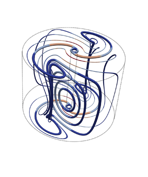
Figure 3 shows the marginally stable 3-D flow and Taylor vortices at  $\eta = \eta _s$. A distinctive feature of the marginally stable 3-D flow, compared to marginally stable axisymmetric Taylor vortices, is that one end of a typical vortex lies near the outer cylinder, but the other end lies at one of the two lines that are offset from the inner cylinder. Also, the critical aspect ratio corresponding to marginally stable 3-D flow is larger than the one corresponding to the Taylor vortices. In fact, with further decrease in the radius ratio, the axisymmetric critical aspect ratio corresponding to the marginally stable 3-D flow grows, whereas the one corresponding to Taylor vortices shrinks, as can been seen from figure 2(a). The decrease of the aspect ratio of the critical perturbations implies that the term
  $\|\boldsymbol {\nabla } \tilde {\boldsymbol {v}}\|_2^2$ increases rapidly as
  $\eta \to 0$, which causes the corresponding critical Taylor number for axisymmetric flows to do the same. This explains why the axisymmetric perturbations are no longer preferred for very low
  $\eta$. At
  $\eta = 0.0188$, the critical Taylor number for the marginally stable Taylor vortices becomes even larger than the one corresponding to the two-dimensional flow (
 $Ta_c^{2D}$).

Figure 3. (a) Selected streamlines of the marginally stable 3-D flow. (b) Selected streamlines of the marginally stable axisymmetric Taylor vortices. In both cases, the radius ratio is  $\eta _s = 0.0556$, and the corresponding critical Taylor numbers are equal. The streamlines are coloured according to the magnitude of the velocity. In both the cases, the velocity field has been scaled such that the maximum magnitude is
  $1$. A typical vortex is shown using relatively thicker lines in both cases. Note that only half the vortex is shown in the axial direction.
Given that we were able to compute the critical Taylor number in case 1 analytically as a function of  $\eta$, it is worth investigating whether the dependence of
  $Ta_c$ on
  $\eta$ in cases 2 and 3 is similar to that of case 1. To do so, we look at figures 1(c) and 1(d), which show the ratios
  $Ta_c^{3D}/Ta_c^{nc}$ and
  $Ta_c^{2D}/Ta_c^{nc}$, respectively. One striking observation is that
  $Ta_c^{3D}/Ta_c^{nc}$ remains within
  $3.6\,\%$ of
  $16.92$ for a fairly large range of radius ratio
  $0.0556 \leqslant \eta \leqslant 1$. So for this range of
  $\eta$,
 \begin{equation} Ta_c^{3D} \approx \frac{16.92 (1 + \eta)^8 (1-\eta)^4}{64 \eta^6} \left(1 + \frac{{\rm \pi}^2}{\log^2 \eta}\right)^2. \end{equation}
However, the same is not valid for case 3, where  $Ta_c^{2D}/Ta_c^{nc}$ varies substantially with
  $\eta$. The spikes in figure 1(d), which are not visible in figure 1(a), correspond to the discrete change in critical azimuthal wavenumber when
  $\eta$ varies, shown in figure 2(b).
For small radius ratio, it is possible to predict the asymptotic behaviour of  $Ta_c^{3D}$ and
  $Ta_c^{2D}$. We find that both
  $Ta_c^{3D}/Ta_c^{nc}$ and
  $Ta_c^{2D}/Ta_c^{nc}$ decrease as
  $\eta \to 0$, as can be seen in figures 1(c) and 1(d). By construction, the asymptotic values of the ratios have to be larger than
  $1$. Therefore, in the small radius ratio limit, we can obtain the asymptotic behaviour of
  $Ta_c^{3D}$ and
  $Ta_c^{2D}$ as
 \begin{equation} Ta_c^{3D} = C_0^{3D} \lim_{\eta \to 0} Ta_c^{nc} = \frac{C_0^{3D} {\rm \pi}^4}{\eta^6 \log^4 \eta}, \quad Ta_c^{2D} = C_0^{2D} \lim_{ \eta \to 0} Ta_c^{nc} = \frac{C_0^{2D} {\rm \pi}^4}{\eta^6 \log^4 \eta}, \quad \text{as}\ \eta \to 0, \end{equation}
where  $1 \leqslant C_0^{3D}, C_0^{2D} < \infty$ are two constants.
4. An analytical bound
In this section, we obtain a simple, suboptimal, analytical bound on the torque, the rate of energy dissipation and the Nusselt number defined in § 2. We use the well-known background method (Doering & Constantin Reference Doering and Constantin1992, Reference Doering and Constantin1994) whose exact formulation in the context of the present problem is given in Appendix A. As usual, we define  $\boldsymbol {U}$ to be the background flow and
  $\boldsymbol {v}$ to be the perturbed flow, such that the total flow is
  $\boldsymbol {u} = \boldsymbol {U} + \boldsymbol {v}$. The background flow
  $\boldsymbol {U}$ is divergence-free and satisfies the same boundary conditions as
  $\boldsymbol {u}$, so the perturbed flow
  $\boldsymbol {v}$ satisfies the homogeneous version of the boundary conditions. For mathematical convenience (see Appendix A), we further define the so-called ‘shifted perturbation’
  $\tilde {\boldsymbol {v}} = \boldsymbol {v} - \boldsymbol {\phi }$ (see (A17)), and we simply refer to
  $\tilde {\boldsymbol {v}}$ as the perturbation from here onward. As shown in Appendix A, a bound on the rate of energy dissipation,
 \begin{equation} \varepsilon \leqslant \frac{1}{({\rm \pi} r_o^2 - {\rm \pi}r_i^2)\,Re\,L} \left[\frac{1}{a (2 -a) }\,\| \boldsymbol{\nabla} \boldsymbol{U}\|_2^2 - \frac{(1-a)^2}{a(2-a)}\,\| \boldsymbol{\nabla} \boldsymbol{u}_{lam}\|_2^2 + 2 {\rm \pi}L\right], \end{equation}
can be obtained for any choice of the background flow for which the functional
 \begin{equation} \mathcal{H} (\tilde{\boldsymbol{v}}) = \frac{2-a}{2 \,Re}\,\| \boldsymbol{\nabla} \tilde{\boldsymbol{v}}\|_2^2 + \underbrace{\int_{V} \tilde{\boldsymbol{v}} \boldsymbol{\cdot} \boldsymbol{\nabla} \boldsymbol{U}_{sym} \boldsymbol{\cdot} \tilde{\boldsymbol{v}} \,{\rm d} \boldsymbol{x}}_{II} \end{equation}
(see (A22)) is positive semi-definite. In (4.1), the constant  $a$ is a balance parameter that takes values between
  $0$ and
  $2$. This bound is identical to the one obtained by Ding & Marensi (Reference Ding and Marensi2019), after noting that they used a different non-dimensionalization. While showing that
  $\mathcal {H} (\tilde {\boldsymbol {v}})$ is non-negative, we do not impose the incompressibility constraint on the perturbations
  $\tilde {\boldsymbol {v}}$ and assume only that
  $\tilde {\boldsymbol {v}}$ satisfies the homogeneous boundary conditions. We make a choice of the background flow
  $\boldsymbol {U}$ for which
 \begin{equation} \boldsymbol{\nabla} \boldsymbol{U}_{sym} = \frac{\boldsymbol{\nabla} \boldsymbol{U} + \boldsymbol{\nabla} \boldsymbol{U}^{\rm T}}{2} \end{equation}
is non-zero only in boundary layers, which are assumed to have thicknesses  $\delta _i$ and
  $\delta _o$ near the inner and outer cylinders, respectively. In particular, the selected background flow
  $\boldsymbol {U}$ is then
 \begin{align} \boldsymbol{U}(r, \theta, z) = U(r)\,\boldsymbol{e}_{\theta} = \begin{cases} \dfrac{\varLambda (r_i + \delta_i) (r - r_i) - (r - r_i - \delta_i)}{\delta_i}\,\boldsymbol{e}_{\theta} & \text{if} \ r_i \leqslant r \leqslant r_i + \delta_i, \\ \varLambda r \boldsymbol{e}_{\theta} & \text{if} \ r_i + \delta_i < r \leqslant r_o - \delta_o, \\ \dfrac{\varLambda (r_o - \delta_o) (r_o - r)}{\delta_o}\,\boldsymbol{e}_{\theta} & \text{if} \ r_o - \delta_o < r \leqslant r_o, \end{cases} \end{align}
where  $\varLambda$ is an
  $O(1)$ constant, i.e. independent of
  $Re$. The decision to allow for different boundary layer thicknesses is inspired from the work of Kumar (Reference Kumar2020), who speculated in the context of helical pipe flows that by doing so, it is possible to capture important geometrical aspects of problems that would otherwise not appear. As we are interested primarily in deriving bounds at asymptotically high Reynolds numbers, for convenience, we define rescaled boundary layer thicknesses as
 \begin{equation} h_i = \frac{\delta_i}{\delta} \quad \text{and} \quad h_o = \frac{\delta_o}{\delta}, \quad \text{where} \ \delta = \frac{1}{Re}, \end{equation}
where, by construction,  $h_i, h_o$ are greater than
  $0$ and are
  $O(1)$. Our goal in this section is to adjust the relative size of the boundary layers (
 $h_i/h_o$) to optimize the bound (4.1) simultaneously for different values of
  $\eta$ in the limit of high Reynolds number.
We start by obtaining a simple estimate for the quantity
 \begin{align} \int_{r_i}^{r_i + \delta_i} |\tilde{v}_r| \, |\tilde{v}_\theta| \,{\rm d}r & = \int_{r_i}^{r_i + \delta_i} \left| \int_{r_i}^{r} \frac{\partial \tilde{v}_r}{\partial r^\prime} \,{\rm d}r^\prime \right| \left| \int_{r_i}^{r} \frac{\partial \tilde{v}_\theta}{\partial r^\prime} \,{\rm d}r^\prime \right| {\rm d}r \nonumber\\ & \leqslant \int_{r_i}^{r_i + \delta_i} (r - r_i) \left[\int_{r_i}^{r_i + \delta_i} \left(\frac{\partial \tilde{v}_r}{\partial r^\prime} \right)^2 {\rm d}r^\prime \right]^{1/2} \left[\int_{r_i}^{r_i + \delta_i} \left(\frac{\partial \tilde{v}_\theta}{\partial r^\prime} \right)^2 {\rm d}r^\prime \right]^{1/2} {\rm d}r \nonumber\\ & = \frac{\delta_{i}^2}{2} \left[\int_{r_i}^{r_i + \delta_i} \left(\frac{\partial \tilde{v}_r}{\partial r^\prime} \right)^2 {\rm d}r^\prime \right]^{1/2} \left[\int_{r_i}^{r_i + \delta_i} \left(\frac{\partial \tilde{v}_\theta}{\partial r^\prime} \right)^2 {\rm d}r^\prime \right]^{1/2} \nonumber\\ & \leqslant \frac{\delta_{i}^2}{4} \int_{r_i}^{r_i + \delta_i} \left(\frac{\partial \tilde{v}_r}{\partial r^\prime} \right)^2 {\rm d}r^\prime + \frac{\delta_{i}^2}{4} \int_{r_i}^{r_i + \delta_i} \left(\frac{\partial \tilde{v}_\theta}{\partial r^\prime} \right)^2 {\rm d}r^\prime. \end{align}
In deriving the result, we have used the fundamental theorem of calculus in the first line and Hölder's inequality in the second line, followed by an integration in  $r$ to obtain the third line. Finally, we used Young's inequality to obtain the last line. In a similar manner, one can also show that
 \begin{equation} \int_{r_o - \delta_o}^{r_o} |\tilde{v}_r| \, |\tilde{v}_\theta| \,{\rm d}r \leqslant \frac{\delta_o^2}{4} \int_{r_o - \delta_o}^{r_o} \left(\frac{\partial \tilde{v}_r}{\partial r^\prime} \right)^2 {\rm d}r^\prime + \frac{\delta_o^2}{4} \int_{r_o - \delta_o}^{r_o} \left(\frac{\partial \tilde{v}_\theta}{\partial r^\prime} \right)^2 {\rm d}r^\prime. \end{equation}
Next, we note that
 \begin{equation} \left| \int_{r = r_i}^{r_i + \delta_i} \tilde{v}_r \tilde{v}_{\theta} \left(\frac{{\rm d} U}{{\rm d}r} - \frac{U}{r}\right) r\,{\rm d}r \right| \leqslant \max_{r_i < r < r_i + \delta_i} \left|\frac{{\rm d}U}{{\rm d}r} - \frac{U}{r}\right| (r_i + \delta_i) \int_{r = r_i}^{r_i + \delta_i} |\tilde{v}_r| \, |\tilde{v}_{\theta}| \,{\rm d}r \end{equation}
and
 \begin{equation} \left| \int_{r = r_o - \delta_o}^{r_o} \tilde{v}_r \tilde{v}_{\theta} \left(\frac{{\rm d} U}{{\rm d}r} - \frac{U}{r}\right) r\,{\rm d}r \right| \leqslant \max_{r_o - \delta_o < r < r_o} \left|\frac{{\rm d} U}{{\rm d}r} - \frac{U}{r}\right| r_o \int_{r = r_o - \delta_o}^{r_o} |\tilde{v}_r| \, |\tilde{v}_{\theta}| \,{\rm d}r. \end{equation}
Using estimates (4.6)–(4.9) along with the expression of the background flow (4.4), we finally obtain a simple bound on term  $II$ in (4.2) as
 \begin{equation} |II| \leqslant \frac{M}{Re}\,\|\boldsymbol{\nabla} \tilde{\boldsymbol{v}}\|_2^2, \end{equation}
where
 \begin{equation} M = \max\left\{\frac{h_i}{4}\,|1 - \varLambda r_i|, \frac{h_o}{4}\,|\varLambda| r_o\right\} + O(\delta). \end{equation}
This shows that the functional  $\mathcal {H}$ is positive semi-definite as long as
 \begin{equation} M \leqslant 1 - \frac{a}{2}. \end{equation}
Using (2.9) and (4.4) in (4.1), we then obtain an upper bound on the dissipation as follows:
 \begin{equation} \varepsilon \leqslant \varepsilon_{b}^a = \frac{2}{a(2-a) (r_o^2 - r_i^2)} \left(\frac{(1 - \varLambda r_i)^2 r_i}{h_i} + \frac{\varLambda^2 r_o^3}{h_o} \right) + O(\delta). \end{equation}
The upper bound obtained is called  $\varepsilon _{b}^a$; we use ‘
 $b$’ in the subscript to signify that it is a bound, and use ‘
 $a$’ in the superscript to signify that it is obtained analytically. In the final step of the procedure, we adjust the values of the unknown parameters
  $h_i$,
  $h_o$,
  $\varLambda$ and
  $a$ to optimize the bound (4.13) while satisfying the constraint (4.12). The optimal values of the parameters, in the limit of high Reynolds number, are
 \begin{equation} \varLambda = \frac{r_i}{r_i^2 + r_o^2}, \quad a = \frac{2}{3}, \quad h_o = \frac{8}{3 \varLambda r_o} \quad \text{and} \quad \frac{h_i}{h_o} = \eta. \end{equation}
Using (4.5a,b) and (2.5), we can now write the optimal choice of boundary layer thicknesses  $\delta _{i}$ and
  $\delta _{o}$ in the limit of
  $Re \to \infty$ (or equivalently
  $Ta \to \infty$) as
 \begin{equation} \delta_i = \frac{8 (1+\eta^2)}{3 \, Re} = \frac{ (1+\eta^2) (1 + \eta)^3}{3 \eta^2 \, Ta^{{1}/{2}}}, \quad \delta_o = \frac{8 (1+\eta^2)}{3 \eta \, Re} = \frac{ (1+\eta^2) (1 + \eta)^3}{3 \eta^3 \, Ta^{{1}/{2}}}. \end{equation}
 The corresponding bound on the dissipation in the limit of  $Re \to \infty$ is then given by
 \begin{equation} \varepsilon_{b, \infty}^a = \frac{27}{32}\,\frac{\eta}{(1 + \eta) (1 + \eta^2)^2}. \end{equation}
Here, we added ‘ $\infty$’ in the subscript to indicate that it is the main term of the bound in the limit
  $Re \to \infty$. Using the relationship (2.24), we obtain an equivalent upper bound on the Nusselt number in the high-Reynolds-number limit as
 \begin{equation} Nu_{b, \infty}^a = \frac{27}{16} \frac{\eta^3}{(1 + \eta)^2 (1 + \eta^2)^2}\,Ta^{1/2}. \end{equation}
This expression contains a dependence on both the Taylor number (the principal flow parameter) and the radius ratio (the geometrical parameter). To separate out the geometrical dependence in (4.17), we define
 \begin{equation} \chi(\eta) = \frac{16 \eta^3}{(1+\eta)^2(1+\eta^2)^2}, \end{equation}
and call it the geometrical scaling of the bound on  $Nu$. This geometrical scaling is defined in such a way that
  $\chi (1) = 1$ (the relevance of
  $\eta = 1$ being that it corresponds to the plane Couette flow case).
Finally, by combining (4.16) with the relation (2.20), we obtain an upper bound on the torque as a function of the Reynolds number:
 \begin{equation} G_{b, \infty}^a = \frac{27 {\rm \pi}}{32}\,\frac{\eta^2 (1+\eta)^2}{(1 - \eta^4)^2}\,Re^2. \end{equation}
Constantin (Reference Constantin1994) had previously obtained a bound on the torque in Taylor–Couette flows by considering a background flow with a single boundary layer. The bound obtained by Constantin is also proportional to  $Re^2$, as in (4.19). But the coefficient in front has a different dependence on the radius ratio
  $\eta$. The reason for this difference is that we chose a background flow with two boundary layers and adjusted their relative thicknesses to optimize the bound. We will see later that this optimization procedure enables us to capture the actual dependence of optimal bounds on the radius ratio.
5. Optimal bounds
In this section, we now proceed to obtain optimal bounds on the bulk quantities, i.e. the best possible bounds within the framework of the background method. As described in § 1, we consider three scenarios, case 1, case 2 and case 3, in which we impose constraints incrementally on the perturbed flow field and obtain numerically the optimal bounds in each case, which allow us to examine systematically the hypothesis stated in the Introduction.
The general development of the background method for Taylor–Couette flow is presented in Appendix A. In what follows, we first describe our numerical algorithm, then proceed to present the results.
5.1. Numerical algorithm
Here, we first describe the general numerical framework used to compute the optimal bounds, and then provide further details of the algorithm in each of the specific cases. Finding the optimal bound begins with the same background method applied to the Taylor–Couette flow as in § 4, which is described in Appendix A. However, instead of using functional inequalities, we now follow the standard route toward optimal bounds, and derive a set of Euler–Lagrange equations that optimal solutions satisfy, given specific constraints in each case. The derivation is presented in Appendix A, and the equations are given in (A28a–d). In general, the Euler–Lagrange equations can have multiple solutions. However, we are interested in finding the unique solution that also satisfies the spectral constraint (A23). To find this particular solution, we use the two-step algorithm first introduced by Wen et al. (Reference Wen, Chini, Dianati and Doering2013) in the context of porous medium convection. A remarkable property of this algorithm is that it eliminates the requirement of numerical continuation (Plasting & Kerswell Reference Plasting and Kerswell2003). As the two-step algorithm can be implemented at any value of the flow parameter, this flexibility has led to wider usage in several other studies of the background method to obtain the optimal bound numerically (Wen et al. Reference Wen, Chini, Kerswell and Doering2015; Wen & Chini Reference Wen and Chini2018; Ding & Marensi Reference Ding and Marensi2019; Lee, Wen & Doering Reference Lee, Wen and Doering2019; Souza, Tobasco & Doering Reference Souza, Tobasco and Doering2020). The first step of the algorithm uses a pseudo-time stepping scheme in which the Euler–Lagrange equations (A28a–d) are converted into a time-dependent system of partial differential equations (PDEs) as follows:
 \begin{align} \frac{\partial \tilde{{v}}_i}{\partial t} = \frac{a}{2 (2-a)}\,\frac{\delta \mathcal{L}}{\delta \tilde{{v}}_i}, \quad \frac{\partial U_\theta}{\partial t} ={-}\frac{a (2-a)}{4 {\rm \pi}L}\,\frac{1}{r}\,\frac{\delta \mathcal{L}}{\delta U_\theta}, \quad \frac{\partial a}{\partial t} ={-} \frac{\delta \mathcal{L}}{\delta a}, \quad \boldsymbol{\nabla} \boldsymbol{\cdot} \tilde{\boldsymbol{v}} = 0, \end{align}
where the index  $i$ ranges over the
  $r$,
$r$,  $\theta$ and
  $z$ components of
  $\tilde {\boldsymbol {v}}$. Steady-state solutions of (5.1a–d) are equivalently solutions of the Euler–Lagrange equations (A28a–d). Note that we multiply the Fréchet derivatives with certain coefficients before introducing the time derivatives on the left-hand side. This makes the coefficient of the linear term (the Laplacian) a constant in the resultant time-dependent PDEs. Also, note that the coefficient in front of the Fréchet derivative with respect to
  $\tilde {\boldsymbol {v}}$ is positive, while the coefficients in front of the Fréchet derivatives with respect to
  $U_\theta$ and
  $a$ are negative. The reason is that we are maximizing the bound with respect to
  $\tilde {\boldsymbol {v}}$ while minimizing it with respect to
  $U_\theta$ and
  $a$.
$a$.
Ding & Marensi (Reference Ding and Marensi2019) proved that if the pseudo-time stepping scheme leads to a steady-state solution, then that solution must be the globally optimal solution of the Euler–Lagrange equations (A28a–d), i.e. the one that leads to optimal bounds. Conveniently, the same proof extends to the case where the perturbed flow satisfies only the homogeneous boundary conditions, and to the case where the perturbed flow is two-dimensional and incompressible. The proof of Ding & Marensi (Reference Ding and Marensi2019) does not guarantee the existence of a steady-state solution to (5.1a–d). But in all the cases that we investigated, the pseudo-time stepping scheme did relax to a steady-state solution.
The second step of the two-step algorithm is a Newton iteration (see Wen et al. Reference Wen, Chini, Kerswell and Doering2015) that has a faster convergence rate than the pseudo-time stepping scheme but requires a good initial guess. Naturally, we use the solution obtained at the end of the pseudo-time stepping scheme as the initial guess.
Solving the Euler–Lagrange equations in case 1 comes with two major simplifications. First, the pressure gradient term in (A28a) disappears, as we do not impose the incompressibility constraint on the perturbation. Second, it can be shown that the optimal perturbation depends only on the radial direction (see Appendix B). With these simplifications, the convergence of the pseudo-time stepping scheme is so rapid that the subsequent Newton iteration is not needed. Therefore, we use only the first step of the two-step algorithm described above. Furthermore, we found that it is also possible to solve the simplified Euler–Lagrange equations analytically in the limit  $Re \to \infty$ using the method of matched asymptotics (solutions are presented in Appendix B).
In case 2, it is also possible to make a simplification. Indeed, Ding & Marensi (Reference Ding and Marensi2019) presented numerical evidence that the optimal solution does not depend on  $\theta$ when the aspect ratio
  $L$ (i.e. the height of the cylinder) is large enough. Therefore, we choose
  $L = 20$, which is sufficiently large to guarantee that the optimal flow is axisymmetric. To solve the system of time-dependent PDEs (5.1a–d), we consider the following Fourier decomposition in the
  $z$-direction:
 \begin{align} \tilde{\boldsymbol{v}} =
\sum_{n = 1}^{N} \begin{bmatrix} \tilde{v}_{r, n}(r, t)
\cos (k_n z) \\ \tilde{v}_{\theta, n}(r, t) \cos (k_n z) \\
\tilde{v}_{z, n}(r, t) \sin (k_n z) \end{bmatrix}, \enspace
\tilde{p} = \sum_{n=1}^N \tilde{p}_n(r, t) \cos (k_n
z), \enspace \text{where}\ k_n = \frac{2 {\rm \pi}n}{L}.
\end{align}
\begin{align} \tilde{\boldsymbol{v}} =
\sum_{n = 1}^{N} \begin{bmatrix} \tilde{v}_{r, n}(r, t)
\cos (k_n z) \\ \tilde{v}_{\theta, n}(r, t) \cos (k_n z) \\
\tilde{v}_{z, n}(r, t) \sin (k_n z) \end{bmatrix}, \enspace
\tilde{p} = \sum_{n=1}^N \tilde{p}_n(r, t) \cos (k_n
z), \enspace \text{where}\ k_n = \frac{2 {\rm \pi}n}{L}.
\end{align}
The radial direction is further discretized using the Chebyshev collocation method. We use a semi-implicit Crank–Nicolson scheme for the time integration, where we treat the linear terms implicitly and use the second-order Adams–Bashforth extrapolation for the nonlinear terms. We use an influence matrix method to solve for the pressure at each time step (see Peyret Reference Peyret2013, p. 236). The code is parallelized using MPI. Note that the pressure  $\tilde {p}$ in (5.2a,b), as compared to the one in Appendix A, has been multiplied with an appropriate factor such that it is precisely the gradient of
  $\tilde {p}$ that appears in the time-evolving PDEs (5.1a–d). Depending on the radius ratio and Taylor number considered, we vary the number modes in the
  $z$-direction from
  $N = 200$ to
  $N = 6000$, and the number collocation points in the
  $r$-direction from
  $120$ to
  $320$.
The numerical strategy for solving the Euler–Lagrange equations in case 3 is similar to case 2 described above. The only difference is that for the 2-D incompressible perturbations, the flow quantities depend on the  $\theta$ direction but are independent of
  $z$. Therefore, we consider the following decomposition instead:
 \begin{equation} \tilde{\boldsymbol{v}} = \sum_{\substack{m={-}M \\ m \neq 0}}^{M} \begin{bmatrix} \tilde{v}_{r, m}(r, t)\,{\rm e}^{{\rm i} m \theta} \\ \tilde{v}_{\theta, m}(r, t)\,{\rm e}^{{\rm i} m \theta} \end{bmatrix}, \quad \tilde{p} = \sum_{\substack{m={-}M \\ m \neq 0}}^M \tilde{p}_m(r, t)\,{\rm e}^{{\rm i} m \theta}. \end{equation}
In this case, depending on the radius ratio and Taylor number considered, we vary the number modes in the  $\theta$-direction from
  $M = 40$ to
  $M = 3000$, and the number collocation points in the
  $r$-direction from
  $120$ to
  $320$.
5.2. Optimal bound results
In this subsection, we present the optimal bounds obtained using the numerical schemes described above for each of the three different sets of constraints on the perturbations. We begin by showing a typical optimal background flow profile at  $\eta = 0.6$ and
  $Ta = 10^6$ in each case in figure 4. For comparison, we have also included the background flow profile constructed in (4.4) to derive the original analytical bound. As can be seen in figure 4, all four background flow profiles vary as
  $c r$, for some constant
  $c$, in the bulk region. This is expected intuitively as this type of background profile makes the sign-indefinite term (which is, in a loose sense, the hardest to control in the bulk region) in the spectral constraint (A23) zero. Near the cylinders, the background flows consist of two thin boundary layers. In order to meet the prescribed boundary conditions, the gradients in these thin layers are large, which makes the sign-indefinite term non-zero. However, as the perturbation has to satisfy the homogeneous boundary conditions, the net contribution from this term will still be smaller than the positive term in (A23) as long as the boundary layer thickness is small enough. In the optimal state, the boundary layers are of just the right size so that the positive term and the sign-indefinite term balance each other and the spectral constraint is marginally satisfied. When moving from case 1 to case 3, the restrictions on the perturbations increase, and this decreases the possibilities in which the sign-indefinite term can be negative. Therefore, the boundary layers become thicker, protruding more into the bulk region.

Figure 4. The optimal background flow  $U_\theta (r)$ at parameter values
  $Ta = 10^6$ and
  $\eta = 0.6$. The orange colour is used for case 1, brown for case 2 and blue for case 3. Also shown, as a black thick line, is the background flow (4.4) used to construct the analytical bound in § 4, with the values of
  $\varLambda$,
  $\delta _i$ and
  $\delta _o$ given by (4.14a–d) in definition (4.4).
Figure 5 shows the optimal bounds on the Nusselt number  $Nu_b$, as a function of the Taylor number
  $Ta$. We denote the bounds as
  $Nu_b^{nc}$ for case 1 (figures 5a,b),
  $Nu_b^{3D}$ for case 2 (figures 5c,d), and
  $Nu_b^{2D}$ for case 3 (figures 5e,f). We cover a wide range of parameters both in radius ratio (from
  $\eta = 0.1$ to
  $\eta = 0.99$) and in Taylor number. In figures 5(a), 5(c) and 5(e), the bound
  $Nu_b$ has been scaled with its expected asymptotic dependence on
  $Ta$, namely
  $Ta^{{1}/{2}}$. The colour and shape of the symbols each correspond to a different radius ratio, as shown in the legend. The symbols in the plots in figure 5 correspond to data points computed using the numerical algorithm from the previous subsection, whereas the solid lines connecting the data points are calculated using interpolation, providing a guide to the eye. For every radius ratio value, the solid line is extended up to the highest Taylor number for which the computation is performed. Beyond this point, we extrapolate using a best fit of the form
 \begin{equation} f(\eta) = A(\eta) + \frac{B(\eta)}{Ta^{\alpha(\eta)}} \end{equation}
applied to the data of  $Nu_b/Ta^{{1}/{2}}$ computed from the last two decades in
  $Ta$. For each value of
  $\eta$, we thus define
  $A(\eta )$ as the asymptotic limit of
  $Nu_b/Ta^{{1}/{2}}$ as
  $Ta \to \infty$. Table 1 summarizes the values of
  $A(\eta )$ obtained from this fitting procedure for different radius ratios. We have added appropriate abbreviations in the superscript of
  $A(\eta )$ to signify the case at hand. We remark that these extrapolations were necessary, especially for the small radius ratios, where the bound on the Nusselt number
  $Nu_b$ converges slowly to its asymptotic scaling in the Taylor number
  $Ta$.
$Ta$.

Figure 5. (a,c,e) The optimal bound  $Nu_b$ compensated with
  $Ta^{{1}/{2}}$ in case 1, case 2 and case 3, respectively, as functions of the Taylor number for a wide range of radius ratios. (b,d, f) The same plots but further scaled with the analytical geometrical scaling
  $\chi (\eta )$ given by (4.18). The collapse of the curves at high Taylor numbers suggests that the bound on Nusselt number
  $Nu_b$ asymptotes to
  $c\,\chi (\eta )\,Ta^{{1}/{2}}$ in all three cases, where the unknown constant
  $c$ is given in (5.5a–c).
Table 1. Variation of the ratio  $A(\eta )/\chi (\eta )$, where
  $A(\eta )$ is from the relation (5.4), and
  $\chi (\eta )$ is given in (4.18), in case 1, case 2 and case 3, where we have respectively added ‘
 $nc$’, ‘
 $3D$’ and ‘
 $2D$’ in the superscript to signify the case. Notice that
  $A(\eta )$ when scaled with
  $\chi (\eta )$ becomes almost invariant in
  $\eta$.

In figures 5(b), 5(d) and 5( f), the bound  $Nu_b$ has been scaled by
  $Ta^{{1}/{2}}$ as well as the geometrical scaling
  $\chi (\eta )$ obtained in (4.18). Note the striking collapse of the different radius ratio curves at high Taylor numbers in all three cases. Correspondingly, we also see from table 1 that the ratio
  $A(\eta )/\chi (\eta )$ is nearly independent of
  $\eta$, with less than
  $1.1\,\%$ variation in the average between the largest and smallest values. This suggests that the geometrical dependence of the bound on the Nusselt number at high Taylor number is
  $\chi (\eta )$ irrespective of the case considered. In case 1, the value of
  $A^{nc}(\eta )/\chi (\eta )$ is close to
  $9/128$, which is the exact asymptotic result that we obtained from the method of matched asymptotics in Appendix C. We also observe from table 1 that the value of
  $A/\chi (\eta )$ in cases 2 and 3 is very close to a constant for
  $\eta > 0.5$, but varies a little more for
  $\eta < 0.5$. This is likely due to the fact that the extrapolation is less accurate at small radius ratio because the computed data are further from being in the asymptotic regime compared with the case when the radius ratio is not small. For this reason, we assume that the average of
  $A(\eta )$ calculated for
  $\eta \geqslant 0.5$ is the correct asymptotic limit of
  $Nu_b/Ta^{{1}/{2}}$ as
  $Ta \to \infty$, and obtain
 $$\begin{gather} Nu_{b, \infty}^{nc} = \frac{9}{8}\,\frac{\eta^3}{(1+\eta)^2(1+\eta^2)^2}\,Ta^{{1}/{2}}, \end{gather}$$
 $$\begin{gather}Nu_{b, \infty}^{3D} = \frac{0.1354 \eta^3}{(1+\eta)^2(1+\eta^2)^2}\,Ta^{{1}/{2}}, \end{gather}$$
 $$\begin{gather}Nu_{b, \infty}^{2D} = \frac{0.0610 \eta^3}{(1+\eta)^2(1+\eta^2)^2}\,Ta^{{1}/{2}}. \end{gather}$$
Here, we have added ‘ $\infty$’ in the subscript to point out that these are the main terms of the optimal bounds in the limit
  $Ta \to \infty$.
In summary, we have shown that for case 1, case 2 and case 3, the optimal bounds are respectively a factor of  $1.5$,
  $12.46$ and
  $27.66$ better than the suboptimal bound (4.17) in the high Taylor number limit. Crucially, this improvement is uniform in the radius ratio
  $\eta$. We had obtained the analytical expression for the geometrical scaling
  $\chi (\eta )$ from a fairly simple suboptimal analytical bound calculated using a choice of background flow with two boundary layers whose thicknesses were adjusted to optimize the bound. During this procedure, we had not applied any constraint on the perturbed flow
  $\tilde {\boldsymbol {v}}$ (other than the homogeneous boundary conditions), and further, used standard calculus inequalities that are known to overestimate the bound on
  $Nu_b$. Consequently, it is not at all self-evident why the optimal bounds should have the same geometrical scaling. The fact that the optimal bounds (5.5a–c), which are up to an order of magnitude better than the suboptimal bound (4.17), preserve the same geometrical dependence on radius ratio is therefore a simple yet remarkable result.
5.3. Wavenumber spectrum of perturbation
In this subsection, we investigate the wavenumber spectrum of the perturbed flow  $\tilde {\boldsymbol {v}}$ with a particular focus on the small-scale structures present in
  $\tilde {\boldsymbol {v}}$. In the optimal state,
  $\tilde {\boldsymbol {v}}$ contains only a finite number of modes, called the critical modes, in either the
  $z$- or
  $\theta$-direction, depending on the case considered, i.e.
 \begin{equation} \tilde{\boldsymbol{v}} = \sum_{n \in K_2} \begin{bmatrix} \tilde{v}_{r, n}(r) \cos (k_n z) \\ \tilde{v}_{\theta, n}(r) \cos (k_n z) \\ \tilde{v}_{z, n}(r) \sin (k_n z) \end{bmatrix} \text{ in case 2}, \quad \tilde{\boldsymbol{v}} = \sum_{m \in K_3} \begin{bmatrix} \tilde{v}_{r, m}(r)\,{\rm e}^{{\rm i} m \theta} \\ \tilde{v}_{\theta, m}(r)\,{\rm e}^{{\rm i} m \theta} \end{bmatrix} \text{ in case 3}, \end{equation}
where  $K_2 \subset \mathbb {N}$ and
  $K_3 \subset \mathbb {Z} \setminus \{0\}$ are finite sets. Moreover, as we will demonstrate below, the smallest scales in the perturbation are present only near the boundaries. It is thus reasonable to hypothesize that the smallest length scale in the perturbation
  $\tilde {\boldsymbol {v}}$ is similar to the boundary layer thickness of the background flow
  $\boldsymbol {U}$. To pursue this idea further, we divide the critical modes present in the perturbation into four different categories. If, for a given critical mode, more than
  $90\,\%$ of the contribution to its
  $L^1({\rm d}r)$ norm comes from the region
 \begin{equation} S_{in} := \left\{r \, | \, r_i \leqslant r \leqslant r_i + \frac{r_o - r_i}{3} \right\}, \end{equation}
then we say that mode is active only near the inner cylinder. Similarly, if it comes from the region
 \begin{equation} S_{out} := \left\{r \, | \, r_o - \frac{r_o - r_i}{3} \leqslant r \leqslant r_o \right\}, \end{equation}
then we say that it is active only near the outer cylinder. Finally, if more than  $90\,\%$ of the contribution comes from regions
  $S_{in}$ and
  $S_{out}$ together, then we say that the mode is active near both the cylinders; otherwise, we say that the mode is active in the bulk. This way of categorizing the modes may seem somewhat arbitrary at first, but looking at the shape of different critical modes, it becomes readily apparent that any other appropriate definition would have led to the same conclusion. We use the following colour scheme to differentiate modes according to our classification: blue for the modes that are active near the inner cylinder, red for the modes that are active near the outer cylinder, green for the modes that are active near both the cylinders, and black for the modes that are active in bulk. Figures 6(b,d, f,h) show the plots of
  $\tilde {v}_{\theta, n_c}(r)$ for critical modes at
  $Ta = 10^8$ and for radius ratios
  $\eta = 0.2, 0.4, 0.6$ and
  $0.8$. We now see that the plots of
  $\tilde {v}_{\theta, n_c}(r)$ provide an unambiguous visual justification of our earlier classification of critical modes into four categories, therefore our classification is robust.

Figure 6. (a,c,e,g) Wavenumbers of the critical modes in the optimal perturbation as a function of  $Ta$ at
  $\eta = 0.2$, 0.4, 0.6 and
  $0.8$, respectively. The colour indicates if the critical mode is active near the inner cylinder (blue), outer cylinder (red) or both cylinders (green), and in the bulk (black), according to the classification given in the main text. The blue and red solid lines are the theoretical predictions for the critical mode with the largest wavenumber active near the inner and outer cylinders (see (5.11a,b)), respectively. (b,d, f,h) Corresponding azimuthal components
  $\tilde {v}_{\theta, n_c}(r)$ of critical modes at the same radius ratios, at
  $Ta = 10^8$.
We first apply this categorization to the optimal perturbations found in case 2, denoting the wavenumber of the critical mode with smallest length scale that is active near the inner cylinder as  $k_{in}^s$, and the one that is active near the outer cylinder as
  $k_{out}^s$. Assuming that our hypothesis about the similarity of the boundary layer thickness in the background flow and the smallest length scale in the perturbation made above is correct, we may expect
 \begin{equation} k_{in}^s \propto \frac{1}{\delta_{i}}, \quad k_{out}^s \propto \frac{1}{\delta_{o}}, \end{equation}
where  $\delta _i$ and
  $\delta _o$ are given by (4.15a,b). Substituting their expressions in the above relation leads to
 \begin{equation} k_{in}^s \propto \frac{\eta^2}{(1+\eta^2)(1+\eta)^3}\,Ta^{{1}/{2}}, \quad k_{out}^s \propto \frac{\eta^3}{(1+\eta^2)(1+\eta)^3}\, Ta^{{1}/{2}}. \end{equation}
From these relations, we obtain the dependence of  $k^s_{in}$ and
  $k^s_{out}$ not only on
  $Ta$, but also on the radius ratio
  $\eta$. In particular, we predict that the smallest length scales in the perturbation should become larger as
  $\eta \to 0$. Furthermore, at a given
  $\eta$, the small-scale structures near the outer cylinder are predicted to be
  $1/\eta$ times larger than the ones near the inner cylinder.
Figures 6(a,c,e,g) show the wavenumbers of the critical modes in the optimal perturbations as a function of the Taylor number for four different radius ratio values  $\eta = 0.2$, 0.4, 0.6 and
  $0.8$, respectively. By fitting these plots, we find that the constant of proportionality in (5.10a,b) that best fits the data at high Taylor numbers is
  $C = 0.244$, therefore we expect
 \begin{equation} k_{in}^s = 0.244\,\frac{\eta^2}{(1+\eta^2)(1+\eta)^3}\,Ta^{{1}/{2}}, \quad k_{out}^s = 0.244\,\frac{\eta^3}{(1+\eta^2)(1+\eta)^3}\, Ta^{{1}/{2}}. \end{equation}
These two relations are plotted in figures 6(a), 6(c), 6(e) and 6(g) with solid blue and red lines, respectively. We see that the smallest length scales in the critical perturbation near the inner and outer boundaries, respectively, indeed follow the relations (5.11a,b). Furthermore, these smallest scales achieve their asymptotic scaling in Taylor number quicker than the corresponding optimal bounds on Nusselt number shown in figure 5, without any need for extrapolation of the data. We therefore argue that (5.11a,b) and figure 6 together provide a strong validation of the analytical predictions from § 4.
We can use similar ideas to predict the scaling of the smallest length scales in optimal perturbations in case 3. Using (4.14a–d), one would anticipate  $m_i^s \propto r_i/\delta _i$ and
  $m_o^s \propto r_o/\delta _o$, where
  $m_i^s$ is the largest wavenumber of a critical mode active near the inner cylinder, and
  $m_o^s$ is the largest wavenumber of a critical mode active near the outer cylinder. The plots in figures 7(a,c,e,g) show the wavenumbers of critical modes in the 2-D optimal perturbations as a function of the Taylor number at radius ratios
  $0.2$,
  $0.4$,
  $0.6$ and
  $0.8$. We apply the same mode identification method, and use the same colour scheme to differentiate the critical modes, as before. From these plots, we can fit the data at high Taylor numbers, to measure the constant of proportionality in the expressions for
  $m_i^s$ and
  $m_o^s$, leading to
 \begin{equation} m_i^s = m_o^s = \frac{0.126\eta^3}{(1-\eta^4)(1+\eta)^2}\,Ta^{{1}/{2}}. \end{equation}
We see that the wavenumbers of the critical mode with smallest length scale that is active near the inner and outer cylinders are equal. The relation (5.12), shown as a solid green line in figures 7(a,c,e,g), does seem to predict the largest wavenumbers at high Taylor numbers correctly.

Figure 7. (a,c,e,g) Wavenumbers  $m_c$ of the critical modes that constitute the 2-D optimal perturbation as a function of the Taylor number for radius ratios
  $\eta = 0.2$, 0.4, 0.6 and
  $0.8$, respectively. We use the same colour scheme as in figure 6 to distinguish different critical modes. The solid green line is the relation (5.12), which predicts the largest critical wavenumber. (b,d, f,h) Plots of
  $\tilde {v}^c_{\theta, m_c}$, the coefficient of
  $\cos m_c \theta$ in the azimuthal component of the velocity, at
  $Ta = 10^8$ and the same radius ratios as in the (a,c,e,g) plots.
As in figure 6, figures 7(b,d, f,h) show the function  $v^c_{\theta, m_c}(r)$, defined as the coefficient of
  $\cos m_c \theta$ in the expression
 \begin{equation} \tilde{v}_{\theta, m_c}(r)\,{\rm e}^{{\rm i} m_c \theta} + \tilde{v}_{\theta, -m_c}(r)\,{\rm e}^{- {\rm i} m_c \theta}, \end{equation}
where  $m_c$ refers to a critical mode. The main difference between the shapes of modes
  $\tilde {v}_{\theta, n_c}(r)$ in figure 6 compared with
  $v^c_{\theta, m_c}(r)$ in figure 7 is that the mean of
  $\tilde {v}_{\theta, m_c}^{c}(r)$ is zero, i.e.
 \begin{equation} \int_{r_i}^{r_o} \tilde{v}_{\theta, m_c}^{c}(r)\,{\rm d}r = 0. \end{equation}
This condition comes from incompressibility, which leads to (5.14) in two dimensions, but does not in three dimensions because the  $z$-component,
  $\tilde {v}_z$, is non-zero. As a result, in two dimensions, modes that are active solely near the cylinders oscillate in the boundary layer to ensure that (5.14) is satisfied.
6. A note on the applicability of the background method
In one of our previous studies (Kumar Reference Kumar2020), we presented a sufficient criterion to determine when the background method can be applied, for a given flow geometry and boundary conditions. We demonstrated that it can be used with any flow problem (tangential-velocity-driven or pressure-driven) with impermeable boundaries, provided that the boundaries have the shape of streamtubes of the flow
 \begin{equation} \boldsymbol{V} = {{\boldsymbol{\mathsf{A}}}} \boldsymbol{x} + \boldsymbol{V}_0, \end{equation}
where  ${{\boldsymbol{\mathsf{A}}}}$ is a constant skew-symmetric tensor,
  $\boldsymbol {V}_0$ is a constant vector, and
  $\boldsymbol {x}$ is the position vector. For these types of problems, one can further show that the upper bound on the dissipation becomes independent of viscosity at high Reynolds numbers. In this section, we explore the complementary question of whether there exist flow configurations for which the background method cannot be applied.
Indeed, the applicability of the background method depends on the existence of an incompressible background flow (which also satisfies the inhomogeneous boundary conditions) such that the following functional is positive semi-definite:
 \begin{equation} \mathcal{H}(\boldsymbol{v}) = \left[\frac{1}{2 \,Re}\,\| \boldsymbol{\nabla} \tilde{\boldsymbol{v}}\|_2^2 + \int_{V} \tilde{\boldsymbol{v}} \boldsymbol{\cdot} \boldsymbol{\nabla} \boldsymbol{U}_{sym} \boldsymbol{\cdot} \tilde{\boldsymbol{v}} \,{\rm d} \boldsymbol{x} + \int_{V} \boldsymbol{U} \boldsymbol{\cdot} \boldsymbol{\nabla} \boldsymbol{U} \boldsymbol{\cdot} \tilde{\boldsymbol{v}} \,{\rm d} \boldsymbol{x}\right], \end{equation}
for any perturbations  $\tilde {\boldsymbol {v}}$ that satisfy the homogeneous boundary conditions. Consequently, proving that the background method cannot be applied reduces to the problem of finding a perturbation or a family of perturbations such that there is no background flow
  $\boldsymbol {U}$ for which
  $\mathcal {H}$ is positive semi-definite.
We start by giving a few examples where the applicability of the background flow can be dismissed rigorously. We first consider the case of Taylor–Couette flow with suction at the inner cylinder. The energy stability analysis of this problem was considered by Gallet, Doering & Spiegel (Reference Gallet, Doering and Spiegel2010). The boundary conditions for this problem are
 \begin{equation} \boldsymbol{u} ={-} \boldsymbol{e}_r + \omega_i r_i \boldsymbol{e}_\theta \text{ at} \ r = r_i, \quad \boldsymbol{u} ={-} \frac{r_i}{r_o} \boldsymbol{e}_r + \omega_o r_o \boldsymbol{e}_\theta \text{ at} \ r = r_o, \end{equation}
where the Reynolds number  $Re$ is defined such that
  $\boldsymbol {u} \boldsymbol {\cdot } \boldsymbol {e}_r = -1$ at the inner cylinder. The non-dimensional angular velocities of the inner and outer cylinders are
  $\omega _i$ and
  $\omega _o$, respectively. In this problem, the flow is constricted to a narrow area as it moves from the outer cylinder (inlet) to the inner cylinder (outlet). We restrict ourselves to two dimensions, but the arguments given below are valid in three dimensions as well. The domain of interest is
  $V = [r_i, r_o] \times [0, 2{\rm \pi} ]$.
We consider a perturbation  $\tilde {\boldsymbol {v}}$ of the form
 \begin{equation} \tilde{\boldsymbol{v}} = (\tilde{v}_r, \tilde{v}_\theta) = \left(0, v_{0} r (r - r_i) (r - r_o)\right), \end{equation}
whose amplitude is  $v_{0}$. Note that
  $\tilde {\boldsymbol {v}}$ satisfies the homogeneous boundary conditions and is incompressible. We now demonstrate that for this perturbation, the spectral constraint can never be satisfied above a certain Reynolds number regardless of the choice of background flow
  $\boldsymbol {U}$.
To show that the spectral constraint (6.2) is not satisfied, we have to show that the second term is negative and that its absolute value is larger than the first term. Being linear in  $\tilde {\boldsymbol {v}}$, the last term can be made arbitrarily small compared with the first two terms by choosing
  $v_{0}$ in (6.4) to be large enough for any given background flow
  $\boldsymbol {U}$. As such, it does not play any role in the following argument.
The calculation of the first term is straightforward:
 \begin{equation} \frac{1}{2 \,Re}\,\| \boldsymbol{\nabla} \tilde{\boldsymbol{v}}\|_2^2 = \frac{\rm \pi}{60\,Re}\,(r_i + r_o) (5r_i^2 + 5r_o^2 + 2) v_{0}^2. \end{equation}
In the calculation of the second term, we take advantage of the fact that the chosen perturbation (6.4) is independent of  $\theta$, so
 \begin{equation} \int_{V} \tilde{\boldsymbol{v}} \boldsymbol{\cdot} \boldsymbol{\nabla} \boldsymbol{U} \boldsymbol{\cdot} \tilde{\boldsymbol{v}} \,{\rm d} \boldsymbol{x} = \int_{r_i}^{r_o} \tilde{v}_\theta^2 \left[\int_{0}^{2 {\rm \pi}}\left(\frac{1}{r}\,\frac{\partial U_\theta}{\partial \theta} + \frac{U_r}{r}\right) {\rm d}\theta \right] r \,{\rm d}r. \end{equation}
Now, using periodicity as well as the incompressibility condition satisfied by the background flow  $\boldsymbol {U}$, the following hold:
 \begin{equation} \int_{0}^{2 {\rm \pi}} \frac{\partial U_\theta}{\partial \theta} \,{\rm d} \theta = 0, \quad \int_{0}^{2 {\rm \pi}} U_r \,{\rm d} \theta ={-} \frac{2 {\rm \pi}r_i}{r}. \end{equation}
Using (6.4) and (6.7a,b) in (6.6) gives
 \begin{equation} \int_{V} \tilde{\boldsymbol{v}} \boldsymbol{\cdot} \boldsymbol{\nabla} \boldsymbol{U} \boldsymbol{\cdot} \tilde{\boldsymbol{v}} \,{\rm d} \boldsymbol{x} ={-} \frac{\rm \pi}{30}\,(r_i^2 + r_i r_o) v_0^2. \end{equation}
From (6.5) and (6.8), we deduce that the spectral constraint (6.2) will not be satisfied if
 \begin{equation} Re > \frac{5r_i^2 + 5r_o^2 + 2}{2 r_i}, \end{equation}
a condition that is, remarkably, independent of the choice of  $\boldsymbol {U}$. Note that in the limit of
  $r_i / r_o \to 1$, the Reynolds number beyond which the method fails goes to infinity. This limit recovers the case of a plane Couette flow with suction and injection at the walls (Doering, Spiegel & Worthing Reference Doering, Spiegel and Worthing2000), where the background method can indeed be applied, so (6.9) is consistent with these results.
A similar type of condition on the Reynolds number can be derived in the problem of the Taylor–Couette flow with injection at the inner cylinder, i.e.
 \begin{equation} \boldsymbol{u} = \boldsymbol{e}_r + \omega_i r_i \boldsymbol{e}_\theta \text{ at} \ r = r_i, \quad \boldsymbol{u} = \frac{r_i}{r_o} \boldsymbol{e}_r + \omega_o r_o \boldsymbol{e}_\theta \text{ at} \ r = r_o. \end{equation}
In this problem, the flow overall expands into a larger area as it moves from the inner cylinder (inlet) to the outer cylinder (outlet). For this case, we can use similar arguments but with the new perturbed flow
 \begin{equation} \tilde{\boldsymbol{v}} = (\tilde{v}_r, \tilde{v}_\theta) = \left(v_0 r (r - r_i) (r - r_o), 0\right). \end{equation}
The perturbation this time is not incompressible but can be shown to yield a negative  $\mathcal {H}(\tilde {\boldsymbol {v}})$ regardless of the background flow
  $\boldsymbol {U}$, for sufficiently large Reynolds number. However, noting that the perturbation (6.11) is radial, one may then expect that an incompressible perturbation, which is composed of vortices stretched in the radial direction, will also yield a negative
  $\mathcal {H}(\tilde {\boldsymbol {v}})$. This observation led us to consider the streamfunction
 \begin{equation} \psi_{v} = v_0 r^2 (r-r_i)^2(r-r_o)^2 \sin m\theta, \quad \text{where } m \in \mathbb{N}. \end{equation}
We define the corresponding velocity field  $\tilde {\boldsymbol {v}} = (\tilde {v}_r, \tilde {v}_\theta )$ as
 \begin{equation} \tilde{v}_r = \frac{1}{r}\,\frac{\partial \psi_v}{\partial \theta}, \quad \tilde{v}_\theta ={-}\frac{\partial \psi_v}{\partial r}. \end{equation}
This velocity field is divergence-free and satisfies the homogeneous boundary conditions at the surface of the cylinders. The streamlines of  $\tilde {\boldsymbol {v}}$ are depicted in figure 8. Next, define a family of rotation operators
  $\mathcal {Q}_{\varphi }:\mathcal {D_\sigma }(V) \to \mathcal {D_\sigma }(V)$, indexed with
  $\varphi$, on the space of divergence-free vector fields that satisfies the homogeneous boundary conditions at
  $\partial V$ as
 \begin{equation} \mathcal{Q}_{\varphi}(\tilde{\boldsymbol{v}})(r, \theta) = \tilde{\boldsymbol{v}}(r, \theta + \varphi) \quad \forall (r, \theta) \in V. \end{equation}
A tedious calculation, first involving an integration in  $\varphi$, and then using the arguments similar to the suction problem above, shows that
 \begin{align} &\int_{0}^{2 {\rm \pi}} \mathcal{H}(\mathcal{Q}_{\varphi}(\tilde{\boldsymbol{v}})) \,{\rm d} \varphi\nonumber\\ &\quad = \frac{{\rm \pi}(r_i + r_o)}{1260}\left[\frac{246 r_i^4 + 138 r_o^4 + 108 r_o^3 + 120 r_i^2 r_o^2 + 108 r_i^2 r_o + 8m^2(r_o^3 - r_i^3) + m^4}{2 \,Re} \right. \nonumber\\ &\qquad \left. \vphantom{\frac{246 r_i^4 + 138 r_o^4 + 108 r_o^3 + 120 r_i^2 r_o^2 + 108 r_i^2 r_o + 8m^2(r_o^3 - r_i^3) + m^4}{2 \,Re}}- r_i (m^2 - 6(r_i^2 + r_o^2))\right]. \end{align}
This calculation implies that if
 \begin{equation} m > \left\lceil \sqrt{6r_i^2 + 6r_o^2} \right\rceil, \end{equation}
where  $\lceil {\cdot } \rceil$ is the ceiling function, then for
 \begin{equation} Re > \frac{246 r_i^4 + 138 r_o^4 + 108 r_o^3 + 120 r_i^2 r_o^2 + 108 r_i^2 r_o + 8m^2(r_o^3 - r_i^3) + m^4}{2 r_i \left(m^2 - 6r_i^2 - 6r_o^2\right)}, \end{equation}
the integral (6.15) is negative, which implies that there is at least one  $\varphi \in [0, 2 {\rm \pi}]$ such that
  $\mathcal {H}(\mathcal {Q}_{\varphi }(\tilde {\boldsymbol {v}})) < 0$. More generally, there exists a set
  $S \subset [0, 2 {\rm \pi}]$, depending on the background flow
  $\boldsymbol {U}$, of positive measure (
 $\mu (S) > 0$) such that
  $\mathcal {H}(\mathcal {Q}_{\varphi }(\tilde {\boldsymbol {v}})) < 0$ for any
  $\varphi \in S$, i.e. the spectral constraint is not satisfied. Note that condition (6.16) is basically saying that the vortices in the incompressible perturbed flow field (6.13a,b) should be stretched in the radial direction, which we expected from the example of the compressible perturbed flow (6.11).

Figure 8. A cartoon of the streamlines of the flow field given by (6.13a,b).
The key message from these two problems is that if there is a converging flow, then one can rule out the applicability of the background method by creating a perturbation whose streamlines are perpendicular to the direction of the mean flow, while in the case of a diverging flow, one can use a perturbation whose streamlines are parallel to the direction of the mean flow instead. Of course, in both cases, we need to make sure that the perturbation satisfies the homogeneous boundary conditions.
Combining these ideas suggests that one cannot apply the background method to flows in a converging–diverging nozzle, because one can choose the perturbation to be composed of vortices that stretch either in the perpendicular direction to the flow in the converging section or parallel to the flow in the diverging section. Using the same arguments, one would then also conjecture that the background method can in general not be applied to flows between rough walls. Indeed, in this case, one can always find vertical sections where the flow expands or compresses, and then one could use the same strategy to choose perturbations for which  $\mathcal {H}(\tilde {\boldsymbol {v}}) < 0$. However, note that in this case, the compression or expansion is small, i.e. the gap width on averages decreases by only a factor
  $(1 - \epsilon )$ in the converging part, or increases by a factor
  $(1 + \epsilon )$ in the diverging part, where
  $\epsilon$ is the non-dimensional roughness scale. This problem is analogous to the converging–diverging nozzle if the Reynolds number is based on the surface roughness
  $\epsilon$. Therefore, for the Reynolds number based on the average gap width, we expect that the spectral constraint (6.2) will not be satisfied if
  $Re \gtrsim \epsilon ^{-1}$.
This still leaves the problem open for the flow systems that do not have a converging or diverging section, for example, flow in tortuous channels. We believe that even for these problems, the spectral constraint will fail to hold past a certain Reynolds number for any background flow. Therefore, we conjecture that the sufficient condition for the applicability of the background method mentioned in the beginning of this section is also a necessary condition.
7. Discussion and conclusion
7.1. Summary and implications
In this paper, we computed optimal bounds on mean quantities in the Taylor–Couette flow problem with a stationary outer cylinder, with particular focus on the dependence of these bounds on the system geometry. Along the way, we studied the energy stability of the laminar flow in § 3. The main finding of this section was that for a value of radius ratio  $r_i/r_o$ below
  $0.0556$, the marginally stable flow at the energy stability threshold is not composed of the well-known axisymmetric Taylor vortices but is instead a fully 3-D flow field.
To uncover the functional dependence of the optimal bounds on the radius ratio at large Taylor number, we began by deriving a suboptimal but analytical bound with the use of standard inequalities and a choice of background flow with two boundary layers (one near the inner cylinder and one near the outer cylinder) whose thicknesses were then adjusted to optimize the bound. We then argued that the dependence on the radius ratio captured by this analytical bound should also be the same for the optimal bounds at large Taylor numbers. We verified this statement systematically by obtaining distinct optimal bounds in three circumstances. In the first case, we imposed no constraints on the perturbation other than the homogeneous boundary conditions (case 1). Next, we allowed for 3-D incompressible perturbations (case 2). And finally, we considered 2-D incompressible perturbations (case 3). In the high Taylor number limit, we see an improvement of  $1.5$,
  $12.46$ and
  $27.66$, respectively, over the analytical bound as we move from case 1 to case 3, and that improvement is the same for all radius ratios. This result is striking and non-trivial because there is no known transformation of variables that makes the Euler–Lagrange equations (A28a–d) of the optimal bounds independent of the radius ratio.
In § 6, we rigorously dismissed the applicability of the background method for two flow problems. The limitation of the background method is previously known in the context of Rayleigh–Bénard convection at infinite Prandtl number (Nobili & Otto Reference Nobili and Otto2017), where it was shown that using a different method, a tighter bound can be obtained as compared to the background method. Here, we have shown that past a certain Reynolds number, no bound can be obtained using the background method applied to Taylor–Couette flow with suction or injection at the inner cylinder, i.e. there is no background flow that satisfies the spectral constraint even when the incompressibility condition on the perturbation is imposed. Generalizing these results then suggests that the spectral condition may not be satisfied for flow problems that contain converging or diverging sections, such as flow in a converging–diverging nozzle or flow between the rough walls. Possibly, the auxiliary functional method (Chernyshenko et al. Reference Chernyshenko, Goulart, Huang and Papachristodoulou2014) could be a way forward to obtain bounds for such problems. The current best-known implementation of this auxiliary functional method to obtain a bound on energy dissipation in flow problems uses only quadratic functionals, in which case it has been shown to be equivalent to the background method (Chernyshenko Reference Chernyshenko2022). However, Chernyshenko (Reference Chernyshenko2022) also proposed potential ways to implement non-quadratic functionals, which might be able to produce a finite bound on the energy dissipation in the problems stated above. Another possible approach, this time numerical, is to consider finite-dimensional truncated models of the actual flow problem, where there is a systematic way to use higher-than-quadratic auxiliary polynomials with the help of the sum-of-squares method (Goulart & Chernyshenko Reference Goulart and Chernyshenko2012; Huang et al. Reference Huang, Chernyshenko, Goulart, Lasagna, Tutty and Fuentes2015; Fantuzzi et al. Reference Fantuzzi, Goluskin, Huang and Chernyshenko2016; Goluskin Reference Goluskin2018; Kumar Reference Kumar2019; Olson et al. Reference Olson, Goluskin, Schultz and Doering2021).
Our study brings to light the significance (or lack of significance, to be more precise) of the incompressibility constraint on the perturbation while calculating optimal bounds, especially in the limit of high Reynolds number, which is generally of interest in turbulent flows. As we showed in the present study, dropping the incompressibility constraint on the perturbations altogether (case 1) still recovers the correct dependence of the bounds on both the principal flow parameter ( $Ta$, or equivalently
  $Re$) and the domain geometry (through the radius ratio). One cannot help but wonder whether the same holds true for other flow problems, including, for instance, the case of convection. It is a fundamental question of concern, as not imposing the incompressibility constraint tremendously decreases the computational cost of the optimal bound calculation. In the particular example studied here, in fact, not imposing the incompressibility condition allowed us to solve the Euler–Lagrange equations analytically using the method of matched asymptotics. This could also be potentially helpful in other studies involving the background method where it is relatively difficult to establish the scaling of the optimal bound even numerically, perhaps because the bounds involve logarithms (Fantuzzi et al. Reference Fantuzzi, Pershin and Wynn2018; Fantuzzi, Nobili & Wynn Reference Fantuzzi, Nobili and Wynn2020) or a scaling other than a simple power law (Kumar et al. Reference Kumar, Arslan, Fantuzzi, Craske and Wynn2022). In such situations, from an analysis point of view, it is usually challenging to decide what combination of the background field and calculus inequalities might be required to obtain the correct asymptotic scaling of the optimal bound. When the bound is obtained numerically instead, it can be difficult to establish its actual functional dependence on the principal flow parameter. Therefore, in these situations, considering case 1 can be very useful as one can try solving the Euler–Lagrange equations analytically using the method of matched asymptotics. These ideas can also be of relevance to other variational approaches, such as the wall-to-wall transport problem (Hassanzadeh, Chini & Doering Reference Hassanzadeh, Chini and Doering2014; Tobasco & Doering Reference Tobasco and Doering2017; Motoki, Kawahara & Shimizu Reference Motoki, Kawahara and Shimizu2018a,Reference Motoki, Kawahara and Shimizub; Doering & Tobasco Reference Doering and Tobasco2019; Souza et al. Reference Souza, Tobasco and Doering2020; Tobasco Reference Tobasco2022; Kumar Reference Kumar2022), which asks the question of what is the maximum heat transfer for a fixed energy or enstrophy budget.
Finally, assuming that the conclusions of this study apply more broadly, case 3 is also relevant to flow problems that are frequently investigated not just in three dimensions but in two dimensions as well, such as Rayleigh–Bénard convection or internally heated convection. For example, it could be interesting to determine how the optimal bounds depend on the shape of the roughness of the wall in 2-D Rayleigh–Bénard convection with rough boundaries, a problem investigated previously by Goluskin & Doering (Reference Goluskin and Doering2016) using the background method.
Before proceeding further, we note that one can also use the direct method of Seis (Reference Seis2015) to derive an upper bound on the Nusselt number with the same Taylor number dependence as in this paper. However, a question of interest could be if a bound with the same geometrical scaling can also be derived. We would expect that if one makes estimates near both the cylinders in Seis's approach, and uses an analogous optimization procedure (similar to this paper), then one may be able to derive a suboptimal bound with the same geometrical scaling as in this paper.
7.2. Comparison with the DNS
We now analyse briefly our results from a more practical point of view, and ask the question of whether the dependence of the Nusselt number on the radius ratio obtained in this paper bears any relationship with that of the actual turbulent flow. Note that the asymptotic dependence of the optimal bound on the Taylor number is known to overestimate the actual Nusselt number in turbulent Taylor–Couette flows by a logarithmic factor in  $Ta$ (Grossmann et al. Reference Grossmann, Lohse and Sun2016). As such, we cannot compare directly our results to the data, but instead merely ask the question of whether the geometric prefactor
  $g(\eta )$ in the expression
  $Nu(\eta,Ta) = g(\eta )\, f(Ta)$ measured in turbulent Taylor–Couette flows bears any resemblance to the prefactor
  $\chi (\eta )$ obtained in our optimal bound calculation; see (4.18).
We first test this idea on the direct numerical simulations (DNS) data from Ostilla-Mónico et al. (Reference Ostilla-Mónico, van der Poel, Verzicco, Grossmann and Lohse2014) and Froitzheim et al. (Reference Froitzheim, Merbold, Ostilla-Mónico and Egbers2019). In figure 9(a), we have plotted  $Nu$ versus
  $Ta$ from these DNS, and in figure 9(b), we show the same data divided by
  $\chi (\eta )$. We see that the rescaled data do become more compact and appear to fall on a single curve. This observation gives us confidence that the geometrical dependence of the bound
  $\chi (\eta )$ obtained in this paper is a good approximation to that of the actual Nusselt number
  $Nu$ measured in turbulent Taylor–Couette flows. However, we note that the data have not yet reached the asymptotic scaling corresponding to the high
  $Ta$ regime, so the comparison at this point remains tentative. We also note that a different prediction for
  $Nu(\eta, Ta)$ has been obtained recently by Berghout et al. (Reference Berghout, Verzicco, Stevens, Lohse and Chung2020) using the idea of Monin–Obukhov theory for thermally stratified turbulent boundary layers. Their scaling of the asymptotic limit of high
  $Ta$ is given as
 \begin{equation} Nu \sim 4 \kappa^2\,\frac{\eta^3}{(1+\eta)^2}\, \frac{Ta^{{1}/{2}}}{\log^2 Ta} = 0.6084\,\frac{\eta^3}{(1+\eta)^2}\, \frac{Ta^{{1}/{2}}}{\log^2 Ta}, \end{equation}
where  $\kappa = 0.39$ is the von Kármán constant. The geometrical dependence in (7.1) differs from
  $\chi (\eta )$ by a factor
  $(1+\eta ^2)^2$. However, it is reassuring to see that both expressions are proportional to
  $\eta ^3$ in the limit of small radius ratio. A definitive answer to the question of whether the geometrical scaling
  $\chi (\eta )$ given by our bound is exact or just an approximation would require a precise comparison with the turbulent data at very high Taylor numbers collected for a range of radius ratios spanning the entire interval
  $(0, 1)$, which is at present a challenge for the numerical computations.

Figure 9. (a) The Nusselt number ( $Nu$) from DNS as a function of the Taylor number (
 $Ta$). (b) The Nusselt number scaled with the geometrical scaling
  $\chi (\eta )$ given by (4.18) as a function of Taylor number. In these plots, the DNS results are taken from Ostilla-Mónico et al. (Reference Ostilla-Mónico, van der Poel, Verzicco, Grossmann and Lohse2014) for
  $\eta = 0.5, 0.714,0.909$, and from Froitzheim et al. (Reference Froitzheim, Merbold, Ostilla-Mónico and Egbers2019) for
  $\eta = 0.357$.
7.3. Further generalizations
We end this paper by discussing a few important consequences and generalizations of our study as well as future outlooks. The first of these consequences concerns the bound on dissipation. The optimal bound on the Nusselt number for case 2 (3-D incompressible perturbations) combined with the relations (2.24) and (2.5) gives us the optimal bound on the dissipation
 \begin{equation} \varepsilon_{b, \infty}^{3D} = 0.0677\,\frac{\eta}{(1 + \eta) (1 + \eta^2)^2}. \end{equation}
This bound tends to  $0.00846$ in the limit
  $\eta \to 1$, which is within
  $1\,\%$ of the optimal bound obtained by Plasting & Kerswell (Reference Plasting and Kerswell2003) for the plane Couette flow, namely
  $0.008553$. The consistency between the two results shows that our work can, in retrospect, be viewed as a generalization of the result of Plasting & Kerswell (Reference Plasting and Kerswell2003) to Taylor–Couette flow for an arbitrary radius ratio.
The second item is related to our previous work (Kumar Reference Kumar2020) on the dependence of the bound on the friction factor  $\lambda$ on the radius of curvature
  $\kappa$ and torsion
  $\tau$ for a pressure-driven flow in a helical pipe. We were able to employ a boundary layer optimization technique together with standard inequalities similar to that used here to obtain the following analytical bound on the friction factor in high
  $Re$ limit:
 \begin{equation} \lambda_{b, \infty}^a = \tfrac{27}{8}\,I(\kappa, \tau), \end{equation}
where
 \begin{equation} I(\kappa, \tau) = \frac{1}{2 {\rm \pi}} \int_{0}^{2 {\rm \pi}} ((1 - \kappa \cos \alpha)^2 + \tau^2)^{3/2} (1 - \kappa \cos \alpha) \,{\rm d} \alpha. \end{equation}
However, the complexity of the helical pipe geometry makes it impossible in practice to compute the corresponding optimal bound. Nevertheless, in the light of results from the present study, and assuming that we captured the geometrical dependence correctly, one can in principle compute the prefactor in a limit where the optimal bound can be computed, namely the case of a straight pipe, for which  $\kappa = \tau = 0$. This bound was computed by Plasting & Kerswell (Reference Plasting and Kerswell2005) to be
  $\lambda _{b, \infty }^{3D}(0,0) = 0.27$, and using this result, we then expect that the optimal bound for helical pipes in the limit of high Reynolds number is
 \begin{equation} \lambda_{b,\infty}^{3D} = 0.27 I(\kappa, \tau). \end{equation}
Finally, the results presented in this paper potentially open the door to solving many important outstanding problems in engineering. Indeed, within that context, we are often interested in finding the optimal geometry of the system or the object involved that minimizes or maximizes a certain flow quantity subject to some physical constraint. These types of problems therefore demand a careful study of the effect of the domain shape on a flow quantity. From this perspective, our study has broader implications. Even though we ruled out the applicability of the background method to a large class of problems (see § 6), this still leaves a number of interesting problems open for analysis. For example, two problems that have been investigated using DNS before, but where an application of the background method can provide further insights, are the Taylor–Couette flow with axisymmetric grooved walls (Zhu et al. Reference Zhu, Ostilla-Mónico, Verzicco and Lohse2016), and pressure-driven flow in a pipe with an elliptic cross-section (Nikitin & Yakhot Reference Nikitin and Yakhot2005). Another problem where the background method has been used previously but capturing the exact domain shape dependence in the bounds was not the primary focus is the flow of fluid in an arbitrary domain driven by moving boundaries (Wang Reference Wang1997). Our study suggests an interesting avenue towards solving these problems, by using the background method together with perturbations that are not assumed to be incompressible, which, as we demonstrated here, can greatly simplify the calculation.
Funding
This paper is dedicated to Charlie Doering, whose work has been instrumental in motivating the author's research. A.K. thanks P. Garaud for a careful read of the paper and for providing comments that improved the quality of the paper. A.K. acknowledges use of the lux supercomputer at UC Santa Cruz, funded by NSF MRI grant AST 1828315.
Declaration of interests
The author reports no conflict of interest.
Appendix A. The background method
In this appendix, we formulate the background method to obtain an upper bound on the quantity
 \begin{equation} \frac{1}{Re}\,\overline{ \| \boldsymbol{\nabla} \boldsymbol{u}\|_2^2} \end{equation}
in Taylor–Couette flow. It is clear from (2.19) that an upper bound on this quantity immediately provides an upper bound on the dissipation  $\varepsilon$.
We begin by writing the total flow field  $\boldsymbol {u}$ as a sum of two divergence-free flow fields:
 \begin{equation} \boldsymbol{u} = \boldsymbol{U} + \boldsymbol{v}. \end{equation}
We call  $\boldsymbol {U}$ the background flow, and require that it satisfies the same boundary conditions as
  $\boldsymbol {u}$, and is a function of only space. We call
  $\boldsymbol {v}$ the perturbation, or perturbed flow, which satisfies homogeneous boundary conditions. The governing equation for the perturbation, obtained by substituting (A2) in (2.3), is given by
 \begin{equation} \frac{\partial \boldsymbol{v}}{\partial t} + \boldsymbol{U} \boldsymbol{\cdot} \boldsymbol{\nabla} \boldsymbol{U} + \boldsymbol{U} \boldsymbol{\cdot} \boldsymbol{\nabla} \boldsymbol{v} + \boldsymbol{v} \boldsymbol{\cdot} \boldsymbol{\nabla} \boldsymbol{U} + \boldsymbol{v} \boldsymbol{\cdot} \boldsymbol{\nabla} \boldsymbol{v} ={-} \boldsymbol{\nabla} p + \frac{1}{Re}\,\nabla^2 \boldsymbol{U} + \frac{1}{Re}\,\nabla^2 \boldsymbol{v}. \end{equation}
We then obtain the evolution equation of the energy in the perturbed flow by taking the dot product of (A3) with  $\boldsymbol {v}$ and integrating over the volume:
 \begin{equation} \frac{{\rm d} \|\boldsymbol{v}\|_2^2}{{\rm d} t} = \frac{1}{Re} \int_{V} \nabla^2 \boldsymbol{U} \boldsymbol{\cdot} \boldsymbol{v} \, {\rm d} \boldsymbol{x} - \frac{1}{Re}\,\|\boldsymbol{\nabla} \boldsymbol{v}\|_2^2 - \int_{V} \boldsymbol{v} \boldsymbol{\cdot} \boldsymbol{\nabla} \boldsymbol{U} \boldsymbol{\cdot} \boldsymbol{v} \,{\rm d} \boldsymbol{x} - \int_{V} \boldsymbol{U} \boldsymbol{\cdot} \boldsymbol{\nabla} \boldsymbol{U} \boldsymbol{\cdot} \boldsymbol{v} \,{\rm d} \boldsymbol{x}. \end{equation}
Now using integration by parts, we can write
 \begin{equation} \int_{V} \nabla^2 \boldsymbol{U} \boldsymbol{\cdot} \boldsymbol{v} \,{\rm d} \boldsymbol{x} ={-} a \int_{V} \boldsymbol{\nabla} \boldsymbol{U} \boldsymbol{\colon} \boldsymbol{\nabla} \boldsymbol{v} \,{\rm d} \boldsymbol{x} + (1-a) \int_{V} \nabla^2 \boldsymbol{U} \boldsymbol{\cdot} \boldsymbol{v} \,{\rm d} \boldsymbol{x}, \end{equation}
where, in the index notation,
 \begin{equation} \boldsymbol{\nabla} \boldsymbol{U} \boldsymbol{\colon} \boldsymbol{\nabla} \boldsymbol{v} = \partial_{i} \boldsymbol{v}_j\,\partial_{i} \boldsymbol{U}_j. \end{equation}
At the same time, one also has the identity
 \begin{equation} \boldsymbol{\nabla} \boldsymbol{U} \boldsymbol{:} \boldsymbol{\nabla} \boldsymbol{v} = \frac{|\boldsymbol{\nabla} \boldsymbol{u}|^2 - |\boldsymbol{\nabla} \boldsymbol{U}|^2 - |\boldsymbol{\nabla} \boldsymbol{v}|^2}{2}. \end{equation}
Using (A5) and (A7) in (A4) leads to
 \begin{align} \frac{{\rm d} \|\boldsymbol{v}\|_2^2}{{\rm d} t} + \frac{a \| \boldsymbol{\nabla} \boldsymbol{u}\|_2^2}{2 \,Re} &= \frac{a \| \boldsymbol{\nabla} \boldsymbol{U}\|_2^2}{2 \,Re} - \frac{2 - a}{2 \,Re}\,\| \boldsymbol{\nabla} \boldsymbol{v}\|_2^2 + \frac{1 - a}{Re} \int_{V} \nabla^2 \boldsymbol{U} \boldsymbol{\cdot} \boldsymbol{v} \, {\rm d} \boldsymbol{x} \nonumber\\ &\quad - \int_{V} \boldsymbol{v} \boldsymbol{\cdot} \boldsymbol{\nabla} \boldsymbol{U} \boldsymbol{\cdot} \boldsymbol{v} \,{\rm d} \boldsymbol{x} - \int_{V} \boldsymbol{U} \boldsymbol{\cdot} \boldsymbol{\nabla} \boldsymbol{U} \boldsymbol{\cdot} \boldsymbol{v} \,{\rm d} \boldsymbol{x}. \end{align}
The introduction of a balance parameter  $a$ in the background formulation goes back to Nicodemus, Grossmann & Holthaus (Reference Nicodemus, Grossmann and Holthaus1997). Now it can be shown within the framework of the background method that the quantity
  $\|\boldsymbol {v}\|_2^2$ is uniformly bounded in time (see Doering & Constantin Reference Doering and Constantin1992, for example). As a result, the long-time average of the time derivative of
  $\|\boldsymbol {v}\|_2^2$ vanishes. Therefore, taking the long-time average of (A8) leads to the bound
 \begin{equation} \frac{1}{Re}\,\overline{ \| \boldsymbol{\nabla} \boldsymbol{u}\|_2^2} \leqslant \frac{1}{Re}\,\| \boldsymbol{\nabla} \boldsymbol{U}\|_2^2 - \frac{2}{a}\,\overline{\mathcal{F} (\boldsymbol{v})}, \end{equation}
where
 \begin{align} \mathcal{F} (\boldsymbol{v}) &= \left[ \frac{2-a}{2\,Re}\,\| \boldsymbol{\nabla} \boldsymbol{v}\|_2^2 - \frac{1 - a}{Re} \int_{V} \nabla^2 \boldsymbol{U} \boldsymbol{\cdot} \boldsymbol{v} \,{\rm d} \boldsymbol{x} \right. \nonumber\\ & \quad \left. {}+ \int_{V} \boldsymbol{v} \boldsymbol{\cdot} \boldsymbol{\nabla} \boldsymbol{U} \boldsymbol{\cdot} \boldsymbol{v} \,{\rm d} \boldsymbol{x} + \int_{V} \boldsymbol{U} \boldsymbol{\cdot} \boldsymbol{\nabla} \boldsymbol{U} \boldsymbol{\cdot} \boldsymbol{v} \,{\rm d} \boldsymbol{x}. \right] \end{align}
This formulation of the background method is general, until this point. From here onwards, we restrict the background flow  $\boldsymbol {U}$ to be unidirectional, of the form
 \begin{equation} \boldsymbol{U} = U_\theta(r)\,\boldsymbol{e}_{\theta}. \end{equation}
At this point, we give the proof of a straightforward but important lemma.
Lemma A.1 Let the domain  $V$ be given by (2.8). Then for a continuous function
  $f:[r_i, r_o] \to \mathbb {R}$ and a divergence-free vector field
  $\boldsymbol {w}:V \to \mathbb {R}^3$ such that
  $\boldsymbol {w} |_{r = r_i} = \boldsymbol {w} |_{r = r_o} = \boldsymbol {0}$ and
  $\boldsymbol {w}$ is periodic in the
  $z$-direction, the following holds:
 \begin{equation} \int_{V} f(r)\,w_r \,{\rm d} \boldsymbol{x} = 0, \end{equation}
where  $w_r$ is the radial component of
  $\boldsymbol {w}$.
Proof. Let
 \begin{equation} F(r, \theta, z) = \int_{r^\prime = r_i}^{r} f(r^\prime) \,{\rm d} r^\prime. \end{equation}
Then we can write
 \begin{equation} \int_{V} f(r)\,w_r \,{\rm d} \boldsymbol{x} = \int_{V} \boldsymbol{\nabla} F \boldsymbol{\cdot} \boldsymbol{w} \,{\rm d} \boldsymbol{x} = \int_{V} \boldsymbol{\nabla} \boldsymbol{\cdot} (F \boldsymbol{w}) \,{\rm d} \boldsymbol{x} = 0, \end{equation}
where we used the divergence theorem and the boundary conditions on  $\boldsymbol {w}$ to obtain the last equality.
The assumption (A11) combined with lemma A.1 implies
 \begin{equation} \int_{V} \boldsymbol{U} \boldsymbol{\cdot} \boldsymbol{\nabla} \boldsymbol{U} \boldsymbol{\cdot} \boldsymbol{v} \,{\rm d} \boldsymbol{x} = 0. \end{equation}
The functional  $\mathcal {F}$ therefore takes the form
 \begin{equation} \mathcal{F} (\boldsymbol{v}) = \left[\frac{2-a}{2 \,Re}\,\| \boldsymbol{\nabla} \boldsymbol{v}\|_2^2 + \int_{V} \boldsymbol{v} \boldsymbol{\cdot} \boldsymbol{\nabla} \boldsymbol{U} \boldsymbol{\cdot} \boldsymbol{v} \,{\rm d} \boldsymbol{x} - \frac{1 - a}{Re} \int_{V} \nabla^2 \boldsymbol{U} \boldsymbol{\cdot} \boldsymbol{v} \,{\rm d} \boldsymbol{x} \right]. \end{equation}
If the infimum of this functional  $\mathcal {F}$ over all the divergence-free vector fields
  $\boldsymbol {v}$ is finite, then it may not be zero as
  $\mathcal {F}$ is not homogeneous due the presence of a linear term. Therefore, similar to Doering & Constantin (Reference Doering and Constantin1998) and Plasting & Kerswell (Reference Plasting and Kerswell2003), we define a shifted perturbation as
 \begin{equation} \tilde{\boldsymbol{v}} = \boldsymbol{v} - \boldsymbol{\phi}, \end{equation}
where both  $\tilde {\boldsymbol {v}}$ and
  $\boldsymbol {\phi }$ are divergence-free and satisfy homogeneous boundary conditions at the surface of the cylinders, and we select
  $\boldsymbol {\phi }$ to eliminate the linear term when the bound (A9) is written in terms of
  $\tilde {\boldsymbol {v}}$.
We substitute (A17) in (A9) and use (A11) and lemma A.1 whenever required. We obtain the following linear term in  $\tilde {\boldsymbol {v}}$:
 \begin{equation} \frac{2}{a \,Re} \int_{V} \left[(2-a)\,\nabla^2 \boldsymbol{\phi} + (1-a)\, \nabla^2 \boldsymbol{U}\right] \boldsymbol{\cdot} \tilde{\boldsymbol{v}} \,{\rm d} \boldsymbol{x}. \end{equation}
Therefore, for this linear term to be zero, we require
 \begin{equation} (2-a)\,\nabla^2 \boldsymbol{\phi} + (1-a)\,\nabla^2 \boldsymbol{U} = 0. \end{equation}
Without loss of generality, we can select the unidirectional solution
 \begin{equation} \boldsymbol{\phi} ={-} \frac{1-a}{2-a} \left[U_\theta - u_{lam, \theta}\right] \boldsymbol{e}_{\theta}. \end{equation}
Using this expression for  $\boldsymbol {\phi }$, the bound in terms of
  $\tilde {\boldsymbol {v}}$ now reads
 \begin{equation} \frac{1}{Re}\,\overline{ \| \boldsymbol{\nabla} \boldsymbol{u}\|_2^2} \leqslant \frac{1}{a (2 -a)\,Re}\,\| \boldsymbol{\nabla} \boldsymbol{U}\|_2^2 - \frac{(1-a)^2}{a(2-a)\,Re}\,\| \boldsymbol{\nabla} \boldsymbol{u}_{lam}\|_2^2 - \frac{2}{a}\,\mathcal{H} (\tilde{\boldsymbol{v}}), \end{equation}
where
 \begin{equation} \mathcal{H} (\tilde{\boldsymbol{v}}) = \left[\frac{2-a}{2\,Re}\,\| \boldsymbol{\nabla} \tilde{\boldsymbol{v}}\|_2^2 + \int_{V} \tilde{\boldsymbol{v}} \boldsymbol{\cdot} \boldsymbol{\nabla} \boldsymbol{U} \boldsymbol{\cdot} \tilde{\boldsymbol{v}} \,{\rm d} \boldsymbol{x}\right]. \end{equation}
If we choose a background flow  $\boldsymbol {U}$ such that the functional
  $\mathcal {H}$ is positive semi-definite on the space of divergence-free vector field
  $\tilde {\boldsymbol {v}}$, i.e.
 \begin{equation} \inf_{\substack{ \tilde{\boldsymbol{v}} \\ \boldsymbol{\nabla} \boldsymbol{\cdot} \tilde{\boldsymbol{v}} = 0}} \mathcal{H} (\tilde{\boldsymbol{v}}) \geqslant 0, \end{equation}
then the bound (A21) is simply
 \begin{equation} \frac{1}{Re}\,\overline{ \| \boldsymbol{\nabla} \boldsymbol{u}\|_2^2} \leqslant \frac{1}{a (2 -a)\,Re}\,\| \boldsymbol{\nabla} \boldsymbol{U}\|_2^2 - \frac{(1-a)^2}{a(2-a)\,Re}\,\| \boldsymbol{\nabla} \boldsymbol{u}_{lam}\|_2^2. \end{equation}
The positive semi-definite condition (A23) on  $\mathcal {H}$ is referred to as the spectral constraint. Since the functional
  $\mathcal {H}$ is quadratic and homogeneous, we can rewrite the spectral constraint as
 \begin{equation} \mathcal{H}
(\tilde{\boldsymbol{v}}) \geqslant 0 \quad \forall
\tilde{\boldsymbol{v}} \text{ such that} \quad
\boldsymbol{\nabla} \boldsymbol{\cdot}
\tilde{\boldsymbol{v}} = 0
\text{ and } \|\tilde{\boldsymbol{v}}\|_2 = 1.
\end{equation}
\begin{equation} \mathcal{H}
(\tilde{\boldsymbol{v}}) \geqslant 0 \quad \forall
\tilde{\boldsymbol{v}} \text{ such that} \quad
\boldsymbol{\nabla} \boldsymbol{\cdot}
\tilde{\boldsymbol{v}} = 0
\text{ and } \|\tilde{\boldsymbol{v}}\|_2 = 1.
\end{equation}
Using the Euler–Lagrange equations, the spectral constraint (A25) is equivalent to the non-negativity of the smallest eigenvalue  $\lambda$ of the following self-adjoint spectral problem:
 $$\begin{gather} \boldsymbol{\nabla} \boldsymbol{\cdot} \tilde{\boldsymbol{v}} = 0, \end{gather}$$
 $$\begin{gather}2 \lambda \tilde{\boldsymbol{v}} = \frac{2-a}{Re}\,\nabla^2 \tilde{\boldsymbol{v}} - 2 \tilde{\boldsymbol{v}} \boldsymbol{\cdot} \boldsymbol{\nabla} \boldsymbol{U}_{sym} - \boldsymbol{\nabla} \tilde{p}. \end{gather}$$
Here,  $\tilde {p}$ and
  $\lambda$ are the Lagrange multipliers for the constraints
  $\boldsymbol {\nabla } \boldsymbol {\cdot } \tilde {\boldsymbol {v}} = 0$ and
  $1 - \|\tilde {\boldsymbol {v}}\|_2^2 = 0$.
Now, to optimize the bound (A21) under the incompressibility constraint on  $\tilde {\boldsymbol {v}}$, we write the following Lagrangian:
 \begin{equation} \mathcal{L} = \frac{1}{a (2 -a)\,Re}\,\| \boldsymbol{\nabla} \boldsymbol{U}\|_2^2 - \frac{(1-a)^2}{a(2-a)\,Re}\,\| \boldsymbol{\nabla} \boldsymbol{u}_{lam}\|_2^2 - \frac{2}{a}\,\mathcal{H} (\tilde{\boldsymbol{v}}) + \int_{V} \tilde{p} \, \boldsymbol{\nabla} \boldsymbol{\cdot} \tilde{\boldsymbol{v}} \,{\rm d} \boldsymbol{x}. \end{equation}
Letting the first variation (the Fréchet derivative) of this functional with respect to  $\tilde {\boldsymbol {v}}$,
  $\tilde {p}$,
  $\boldsymbol {U}$ and
  $a$ tend to zero leads to
 $$\begin{gather} \frac{\delta \mathcal{L}}{\delta \tilde{\boldsymbol{v}}} = \frac{2 (2-a)}{a \,Re}\,\nabla^2 \tilde{\boldsymbol{v}} - \frac{4}{a}\,\tilde{\boldsymbol{v}} \boldsymbol{\cdot} \boldsymbol{\nabla} \boldsymbol{U}_{sym} - \boldsymbol{\nabla} \tilde{p} = 0, \end{gather}$$
 $$\begin{gather}\frac{\delta
\mathcal{L}}{\delta \tilde{p}} = \boldsymbol{\nabla}
\boldsymbol{\cdot} \tilde{\boldsymbol{v}} = 0,
\end{gather}$$
$$\begin{gather}\frac{\delta
\mathcal{L}}{\delta \tilde{p}} = \boldsymbol{\nabla}
\boldsymbol{\cdot} \tilde{\boldsymbol{v}} = 0,
\end{gather}$$ $$\begin{gather}\frac{\delta \mathcal{L}}{\delta U_\theta} ={-}\frac{4 {\rm \pi}L}{a (2-a)\, Re} \left(r\,\frac{{\rm d}^2 U_\theta}{{\rm d} r^2} + \frac{{\rm d} U_\theta}{{\rm d} r} - \frac{U_\theta}{r}\right) + \frac{1}{ r}\,\frac{{\rm d}}{{\rm d}r} \left(\frac{2 r^2}{a} \int_{\theta = 0}^{2 {\rm \pi}} \int_{z = 0}^{L} \tilde{v}_r \tilde{v}_\theta \,{\rm d} \theta \,{\rm d} z\right) = 0, \end{gather}$$
 $$\begin{gather}\frac{\delta
\mathcal{L}}{\delta a} = \frac{2(a-1)}{a^2(2-a)^2\,Re}
\left(\!\|\boldsymbol{\nabla} \boldsymbol{U}\|_2^2 -
\|\boldsymbol{\nabla} \boldsymbol{u}_{lam}\|_2^2\!\right) +
\frac{2}{a^2} \left(\!\frac{1}{Re}\,\|\boldsymbol{\nabla}
\tilde{\boldsymbol{v}}\|_2^2 + \int_{V}
\tilde{\boldsymbol{v}} \boldsymbol{\cdot}
\boldsymbol{\nabla} \boldsymbol{U} \boldsymbol{\cdot}
\tilde{\boldsymbol{v}} \,{\rm d} \boldsymbol{x} \!\right) =
0.
\end{gather}$$
$$\begin{gather}\frac{\delta
\mathcal{L}}{\delta a} = \frac{2(a-1)}{a^2(2-a)^2\,Re}
\left(\!\|\boldsymbol{\nabla} \boldsymbol{U}\|_2^2 -
\|\boldsymbol{\nabla} \boldsymbol{u}_{lam}\|_2^2\!\right) +
\frac{2}{a^2} \left(\!\frac{1}{Re}\,\|\boldsymbol{\nabla}
\tilde{\boldsymbol{v}}\|_2^2 + \int_{V}
\tilde{\boldsymbol{v}} \boldsymbol{\cdot}
\boldsymbol{\nabla} \boldsymbol{U} \boldsymbol{\cdot}
\tilde{\boldsymbol{v}} \,{\rm d} \boldsymbol{x} \!\right) =
0.
\end{gather}$$In general, these equations do not have a unique solution. However, the solution to these equations for which the background flow also satisfies the spectral constraint (A23), or equivalently, all the eigenvalues of the eigenvalue problem (A26a,b) are non-negative, is unique.
Appendix B. A useful lemma
Here, we prove that the marginally stable perturbations in the energy stability analysis of § 3 or optimal perturbations in § 5 depend on radius only when they are not required to be incompressible.
Lemma B.1 Let  $\mathcal {D}(V)$ be the set of smooth velocity fields (not necessarily incompressible) that satisfy the homogeneous boundary conditions. For a given choice of the balance parameter
  $0 < a < 2$ and of the unidirectional background flow
  $\boldsymbol {U} = U_\theta (r)\, \boldsymbol {e}_\theta$, the functional
  $\mathcal {H}(\tilde {\boldsymbol {v}})$ (given by (A22)) achieves a minimum when
  $\tilde {\boldsymbol {v}}$ is a function of the radial direction only. Furthermore, if the background flow satisfies
  ${\rm d}U_\theta / {\rm d}r - U_\theta /r \leqslant 0$, then the optimal perturbed flow corresponds to
  $\tilde {v}_r = \tilde {v}_\theta$.
Remark B.2 Although we do not prove that the optimal background flow satisfies  ${\rm d}U_\theta / {\rm d}r - U_\theta /r \leqslant 0$, this condition was found to hold in every numerical computation of optimal bounds in all the three cases considered in our paper, as well as for the choice of the background flow in analytical construction presented in § 4. Therefore, it is natural to make the assumption that
  ${\rm d}U_\theta / {\rm d}r - U_\theta /r \leqslant 0$.
Proof. In the first part of the lemma, it is sufficient to show that for every  $\tilde {\boldsymbol {v}} \in \mathcal {D}(V)$ there exist
  $\tilde {\boldsymbol {v}}_0 \in \mathcal {D}(V)$ with
  $\tilde {\boldsymbol {v}}_0(\boldsymbol {x}) = \tilde {\boldsymbol {v}}_0(r)$ such that
  $\mathcal {H}(\tilde {\boldsymbol {v}}_0) \leqslant \mathcal {H}(\tilde {\boldsymbol {v}})$:
 \begin{align}
\mathcal{H} (\tilde{\boldsymbol{v}}) & =
\left[\frac{2-a}{2\,Re}\,\| \boldsymbol{\nabla}
\tilde{\boldsymbol{v}}\|_2^2 + \int_{V}
\tilde{\boldsymbol{v}} \boldsymbol{\cdot}
\boldsymbol{\nabla} \boldsymbol{U} \boldsymbol{\cdot}
\tilde{\boldsymbol{v}} \,{\rm d} \boldsymbol{x}\right]
\nonumber\\ & = \left[\int_{z = 0}^{L} \int_{\theta = 0}^{2
{\rm \pi}}\left( \int_{r = r_i}^{r_o} \frac{2-a}{2\,Re}\,|
\boldsymbol{\nabla} \tilde{\boldsymbol{v}}|^2 +
\tilde{\boldsymbol{v}} \boldsymbol{\cdot}
\boldsymbol{\nabla} \boldsymbol{U} \boldsymbol{\cdot}
\tilde{\boldsymbol{v}} \,r \,{\rm d} r \right) {\rm d}
\theta \,{\rm d} z \right] \nonumber\\
& \geqslant \left[\int_{z = 0}^{L} \int_{\theta = 0}^{2 {\rm \pi}}
\inf_{\substack{ 0 \leqslant \theta \leqslant 2 {\rm \pi}\nonumber\\
0 \leqslant z \leqslant L}} \left( \int_{r =
r_i}^{r_o} \frac{2-a}{2\,Re}\,| \boldsymbol{\nabla}
\tilde{\boldsymbol{v}}|^2 + \tilde{\boldsymbol{v}}
\boldsymbol{\cdot} \boldsymbol{\nabla} \boldsymbol{U}
\boldsymbol{\cdot} \tilde{\boldsymbol{v}} \,r \,{\rm d} r
\right) {\rm d} \theta \,{\rm d} z \right] \nonumber\\
&= \mathcal{H} (\tilde{\boldsymbol{v}}_0),
\end{align}
\begin{align}
\mathcal{H} (\tilde{\boldsymbol{v}}) & =
\left[\frac{2-a}{2\,Re}\,\| \boldsymbol{\nabla}
\tilde{\boldsymbol{v}}\|_2^2 + \int_{V}
\tilde{\boldsymbol{v}} \boldsymbol{\cdot}
\boldsymbol{\nabla} \boldsymbol{U} \boldsymbol{\cdot}
\tilde{\boldsymbol{v}} \,{\rm d} \boldsymbol{x}\right]
\nonumber\\ & = \left[\int_{z = 0}^{L} \int_{\theta = 0}^{2
{\rm \pi}}\left( \int_{r = r_i}^{r_o} \frac{2-a}{2\,Re}\,|
\boldsymbol{\nabla} \tilde{\boldsymbol{v}}|^2 +
\tilde{\boldsymbol{v}} \boldsymbol{\cdot}
\boldsymbol{\nabla} \boldsymbol{U} \boldsymbol{\cdot}
\tilde{\boldsymbol{v}} \,r \,{\rm d} r \right) {\rm d}
\theta \,{\rm d} z \right] \nonumber\\
& \geqslant \left[\int_{z = 0}^{L} \int_{\theta = 0}^{2 {\rm \pi}}
\inf_{\substack{ 0 \leqslant \theta \leqslant 2 {\rm \pi}\nonumber\\
0 \leqslant z \leqslant L}} \left( \int_{r =
r_i}^{r_o} \frac{2-a}{2\,Re}\,| \boldsymbol{\nabla}
\tilde{\boldsymbol{v}}|^2 + \tilde{\boldsymbol{v}}
\boldsymbol{\cdot} \boldsymbol{\nabla} \boldsymbol{U}
\boldsymbol{\cdot} \tilde{\boldsymbol{v}} \,r \,{\rm d} r
\right) {\rm d} \theta \,{\rm d} z \right] \nonumber\\
&= \mathcal{H} (\tilde{\boldsymbol{v}}_0),
\end{align}
where  $\tilde {\boldsymbol {v}}_0 (\boldsymbol {x}) = \tilde {\boldsymbol {v}}(r, \theta _0, z_0)$, and
  $\theta _0$,
  $z_0$ corresponds to the values for which the infimum in the third line is achieved.
In the second part, for every perturbation  $\tilde {\boldsymbol {v}} = (\tilde {v}_r, \tilde {v}_\theta )$, we define a modified perturbation
 \begin{equation} \hat{\boldsymbol{v}} = \left(\frac{\sqrt{\tilde{v}_r^2 + \tilde{v}_\theta^2}}{\sqrt{2}}, \frac{\sqrt{\tilde{v}_r^2 + \tilde{v}_\theta^2}}{\sqrt{2}}\right). \end{equation}
So if the initial perturbations  $\tilde {\boldsymbol {v}}$ are weakly differentiable in space, then so is the modified perturbation
  $\hat {\boldsymbol {v}}$. Therefore, all the operations below apply. For this modified perturbation, we have
 \begin{align} \| \boldsymbol{\nabla} \boldsymbol{\hat{v}}\|_2^2 & = \frac{\tilde{v}_r^2}{\tilde{v}_r^2 + \tilde{v}_\theta^2} \left(\frac{\partial \tilde{v}_r}{\partial r}\right)^2 + \frac{\tilde{v}_\theta^2}{\tilde{v}_r^2 + \tilde{v}_\theta^2} \left(\frac{\partial \tilde{v}_\theta}{\partial r}\right)^2 + \frac{\tilde{v}_r \tilde{v}_\theta}{\tilde{v}_r^2 + \tilde{v}_\theta^2}\, \frac{\partial \tilde{v}_r}{\partial r}\,\frac{\partial \tilde{v}_\theta}{\partial r} + \frac{\tilde{v}_r^2 + \tilde{v}_\theta^2}{r} \nonumber\\ & \leqslant \left(\frac{\partial \tilde{v}_r}{\partial r}\right)^2 + \left(\frac{\partial \tilde{v}_\theta}{\partial r}\right)^2 + \frac{\tilde{v}_r^2 + \tilde{v}_\theta^2}{r} = \| \boldsymbol{\nabla} \tilde{\boldsymbol{v}}\|_2^2, \end{align}
where we used Young's inequality on the third term on the right-hand side in the first line to obtain the second line. Now the assumption on  $U_\theta$ implies
 \begin{equation} \frac{\tilde{v}_r^2 + \tilde{v}_\theta^2}{2} \left(\frac{{\rm d}U_\theta}{{\rm d}r} - \frac{U_\theta}{r} \right) \leqslant \tilde{v}_r \tilde{v}_\theta \left(\frac{{\rm d}U_\theta}{{\rm d}r} - \frac{U_\theta}{r} \right), \end{equation}
again through the use of Young's inequality. Combining (B3) and (B4) with the definition of  $\mathcal {H}(\boldsymbol {v})$ leads to
 \begin{equation} \mathcal{H}(\hat{\boldsymbol{v}}) \leqslant \mathcal{H}(\tilde{\boldsymbol{v}}). \end{equation}
Finally, noting that  $\hat {v}_r = \hat {v}_\theta$ proves the lemma.
Appendix C. Analytical solution of the Euler–Lagrange equations in case 1 at high Reynolds number
Before writing the Euler–Lagrange equations, we recall the simplifications pertaining to case 1. From lemma B.1, we note that the optimal perturbations depend only on the radial direction, and that  $\tilde {v}_r = \tilde {v}_\theta$. Finally, noting that the Lagrangian
  $\mathcal {L}$ in case 1 does not involve the pressure term, as we do not impose the incompressibility condition, the simplified Euler–Lagrange equations (A28a–d) in case 1 are given by
 $$\begin{gather} \frac{2-a}{Re} \left(\frac{{\rm d}^2 \tilde{v}_r}{{\rm d} r^2} + \frac{1}{r}\,\frac{{\rm d} \tilde{v}_r}{{\rm d} r} - \frac{\tilde{v}_r}{r^2}\right) - \tilde{v}_{r} \left(\frac{{\rm d} U_\theta}{{\rm d} r} - \frac{U_\theta}{r}\right) =0, \end{gather}$$
 $$\begin{gather}-\frac{1}{(2-a)\,Re} \left(r\,\frac{{\rm d}^2 U_\theta}{{\rm d} r^2} + \frac{{\rm d} U_\theta}{{\rm d} r} - \frac{U_\theta}{r}\right) + \frac{1}{r}\,\frac{{\rm d} (r^2\tilde{v}_r^2)}{{\rm d}r} = 0, \end{gather}$$
 $$\begin{gather}\frac{a-1}{(2-a)^2\,Re} \left(\|\boldsymbol{\nabla} \boldsymbol{U}\|_2^2 - \|\boldsymbol{\nabla} \boldsymbol{u}_{lam}\|_2^2\right) + \frac{1}{Re}\,\|\boldsymbol{\nabla} \tilde{\boldsymbol{v}}\|_2^2 + \int_{V} \tilde{\boldsymbol{v}} \boldsymbol{\cdot} \boldsymbol{\nabla} \boldsymbol{U} \boldsymbol{\cdot} \tilde{\boldsymbol{v}} \,{\rm d} \boldsymbol{x} = 0. \end{gather}$$
These equations need to be solved with boundary conditions
 $$\begin{gather} U_\theta = 1, \quad \tilde{v}_r = 0 \quad \text{at} \ r = r_i, \end{gather}$$
 $$\begin{gather}U_\theta = 0, \quad \tilde{v}_r = 0 \quad \text{at} \ r = r_o. \end{gather}$$
As  $\tilde {v}_z$ does not enter into the computations, it can be taken to be zero; as such,
  $\tilde {\boldsymbol {v}}$ here should be understood as
  $(\tilde {v}_r, \tilde {v}_r, 0)$.
These equations can be solved using the method of matched asymptotics as described below. We consider three different regions: the inner boundary layer, the bulk and the outer boundary layer. We use the following scaled coordinates for the inner and outer boundary layers, respectively:
 \begin{equation} s_i = \frac{r - r_i}{\delta}, \quad s_o = \frac{r_o - r}{\delta}, \end{equation}
where
 \begin{equation} \delta = \frac{1}{Re}. \end{equation}
We will use  $in$,
$in$,  $bulk$ and
  $out$ in the superscript of the variables to indicate in which region the variable is being considered. Before proceeding further, we make the following change of variables:
 \begin{equation} U = \frac{U_\theta}{r}, \quad \tilde{v} = r \tilde{v}_r. \end{equation}
Next, we write separate expansions for the variables in each of the three different regions as
 $$\begin{gather} \tilde{v}^{in}(s_i) = \tilde{v}_{0}^{in}(s_i) + \delta \, \tilde{v}_{1}^{in}(s_i) + \delta^2 \, \tilde{v}_{2}^{in}(s_i) + \cdots, \end{gather}$$
 $$\begin{gather}\tilde{v}^{bulk}(r) = \tilde{v}_{0}^{bulk}(r) + \delta \, \tilde{v}_{1}^{bulk}(r) + \delta^2 \, \tilde{v}_{2}^{bulk}(r) + \cdots, \end{gather}$$
 $$\begin{gather}\tilde{v}^{out}(s_o) = \tilde{v}_{0}^{out}(s_o) + \delta \, \tilde{v}_{1}^{out}(s_o) + \delta^2 \, \tilde{v}_{2}^{out}(s_o) + \cdots. \end{gather}$$
A similar expansion can be written for  $U$. Finally, we also use a simple expansion for the balance parameter
 \begin{equation} a = a_0 + \delta a_1 + \delta^2 a_2 + \cdots. \end{equation}
Substituting the change of variables (C5a,b) and the series expansions of these new variables in (C1a–c), one can find the leading-order equations in different regions, which then need to be solved with the boundary conditions (C2a,b) and the following matching conditions:
 $$\begin{gather} U_{0}^{in}(s_i \to \infty) = U_{0}^{bulk}(r = r_i), \quad U_{0}^{bulk}(r = r_o) = U_{0}^{out}(s_o \to \infty), \end{gather}$$
 $$\begin{gather}\tilde{v}_{0}^{in}(s_i \to \infty) = \tilde{v}_{0}^{bulk}(r = r_i), \quad \tilde{v}_{0}^{bulk}(r = r_o) = \tilde{v}_{0}^{out}(s_o \to \infty). \end{gather}$$
Upon solving the resultant set of equations, we find that the leading-order term in the background flow in the three different regions is given by
 $$\begin{gather} U_{\theta}^{in} = \frac{r}{r_i}\left(1 - \frac{4 \sqrt{2}}{3}\,\alpha \tanh \left(\frac{\alpha s_i}{\sqrt{2}}\right) \right) + O\left(\delta\right), \end{gather}$$
 $$\begin{gather}U_{\theta}^{bulk} = \frac{r_i r}{r_i^2 + r_o^2} + O\left(\delta\right), \end{gather}$$
 $$\begin{gather}U_{\theta}^{out} = \frac{r}{r_o}\left(\frac{4 \sqrt{2}}{3}\,\beta \tanh \left(\frac{\beta s_o}{\sqrt{2}}\right) \right) + O\left(\delta\right), \end{gather}$$
whereas the perturbed flow field is given by
 $$\begin{gather} \tilde{v}_{r}^{in} = \tilde{v}_{\theta}^{in} = \frac{\alpha r_i}{r} \tanh \left(\frac{\alpha s_i}{\sqrt{2}}\right) + O\left(\delta\right), \end{gather}$$
 $$\begin{gather}\tilde{v}_{r}^{out} = \tilde{v}_{\theta}^{out} = \frac{\beta r_o}{r} \tanh \left(\frac{\beta s_o}{\sqrt{2}}\right) + O\left(\delta\right), \end{gather}$$
 $$\begin{gather}\tilde{v}_{r}^{bulk} = \tilde{v}_{\theta}^{bulk} = \left(\frac{3 r_i r_o^2}{4 \sqrt{2} (r_i^2 + r_o^2)} \right) \frac{1}{r} + O\left(\delta\right), \end{gather}$$
where  $\alpha$ and
  $\beta$ depend on
  $\eta$ and are given by
 \begin{equation} \alpha = \frac{3}{4 \sqrt{2}}\,\frac{1}{1 + \eta^2}, \quad \beta = \frac{3}{4 \sqrt{2}}\,\frac{\eta}{1 + \eta^2}. \end{equation}
The balance parameter takes the value  $a = 2/3 + O(\delta )$. This optimal value
  $a = 2/3$ of the balance parameter, in the limit of large
  $Re$, is also observed numerically by Ding & Marensi (Reference Ding and Marensi2019) (and corresponds to
  $3/2$ in their non-dimensionalization) as well as in cases 2 and 3 in our study. Using the expression of the background flow (C9a–c) in (A24), and the relationships between different mean quantities (2.19) and (2.24), the leading-order term in the bound on the Nusselt number in the limit of high Reynolds number (or equivalently, high Taylor number), is given by
 \begin{equation} Nu_{b}^{nc} = \frac{9}{8}\,\frac{\eta^3}{(1 + \eta)^2 (1 + \eta^2)^2}\, Ta^{1/2}. \end{equation}
This bound is  $2/3$ of the bound (4.17) obtained using standard inequalities. This improvement has also been confirmed by the numerical results.


 Open access