


1. Introduction
The interaction between surfaces and pure fluid/mixtures has major applications in laboratory experiments as well as in industry, like when chromatography or adsorption processes are operated. Two interface-driven phenomena, nowadays known as diffusioosmosis and diffusiophoresis, were described by Derjaguin and coauthors in 1947 (Derjaguin et al. Reference Derjaguin, Sidorenkov, Zubashchenkov and Kiseleva1947). The researchers observed that solutions in a capillary tube can flow relative to the fixed wall if a gradient in solute concentration is applied. Furthermore, the authors noted that particles may move spontaneously in a fluid mixture because of a concentration gradient of a different substance. These observations are instances of diffusioosmosis and diffusiophoresis, respectively.
Diffusiophoresis is present in applications ranging from particle separation in microfluidics (Shin Reference Shin2020) to oil extraction (Velegol et al. Reference Velegol, Garg, Guha, Kar and Kumar2016). This phenomenon is also believed to influence several natural processes, such as intracellular transport of viral DNA and protein transport across membrane pores (Velegol et al. Reference Velegol, Garg, Guha, Kar and Kumar2016). Most of the early models for diffusiophoresis made strong simplifying assumptions, like an infinitesimally thin interface–solute interaction range (Derjaguin et al. Reference Derjaguin, Sidorenkov, Zubashchenkov and Kiseleva1947). Furthermore, many of the later papers focus on adsorbing solutes (Anderson & Prieve Reference Anderson and Prieve1984), and are not valid for repulsive interface–solute interactions. Recent modelling works that are not restricted to adsorption keep some simplifying assumptions, such as neglecting solute advection (Brady Reference Brady2011; Marbach, Yoshida & Bocquet Reference Marbach, Yoshida and Bocquet2020). These assumptions will be waived in this paper.
Apart from this, the literature does not pay much attention to the intrinsic transient character of diffusiophoresis. Phoretic systems are inherently transient because the particle experiences different bulk solute concentrations as it moves. However, authors often argue that the migration speed of the particle is slow enough so that the concentration can be always considered at steady state (the quasi-steady state approximation) (Anderson & Prieve Reference Anderson and Prieve1984; Brady Reference Brady2011; Marbach et al. Reference Marbach, Yoshida and Bocquet2020). For sufficiently large solute diffusion coefficients (infinite diffusivity), this approximation holds and solute transport via convection can also be neglected (Brady Reference Brady2011; Marbach et al. Reference Marbach, Yoshida and Bocquet2020). In this case, the phoretic velocity depends only on the externally imposed solute gradient, and not on the absolute value of solute concentration in the bulk. However, if convection is taken into account, the diffusiophoretic velocity depends on the bulk solute concentration (Anderson & Prieve Reference Anderson and Prieve1984).
Such a dependency already highlights the transient character of these systems: as the particle moves, the bulk concentration changes, and so does its velocity. But even more interesting transient aspects of diffusiophoresis can be studied if the quasi-steady hypothesis is dropped. For example, one may be interested in knowing whether the phoretic flow depends on the initial conditions after a long time. For quasi-steady systems, this dependency does not occur because the solute concentration profile is always in its steady form. However, the matter is not trivial when the dependency on time is considered: indeed, the fact that the particle is always moving and that its velocity is always changing means that a steady state is never achieved. Even if fluid and particle inertia are neglected, two systems with different initial conditions (e.g. different initial concentration profiles) will evolve differently. The differences in the solute concentration profiles affect the fluid velocity field, as the latter depends on the former. This effect is entangled with the dependency of concentration on the velocity field when advection is considered. Therefore, a phoretic system may or may not forget its initial state after a long time. To the best of the authors’ knowledge, this question has never been addressed. Hereafter, we use the term fully developed state to refer to the hypothetical systems whose properties no longer depend on the initial state. This is different from the equilibrium state, which is an approximation that considers the particle at mechanical equilibrium.
The investigation on fully developed states will be assisted by numerical simulations. The use of such simulations to study phoretic systems is not unprecedented. Indeed, they are useful to support or illustrate theoretical findings. For example, Ault, Shin & Stone (Reference Ault, Shin and Stone2018) studied the dynamics of a fluid/particle/solute system comprised in a narrow channel. In their study, numerical simulations were used to validate the series expansion approach employed to derive analytical solutions for the two-dimensional velocity, solute concentration and particle concentration profiles. Another set of simulations illustrates the shift away from one-dimensional predictions as the channel aspect ratio increases. In addition, simulations in conjunction with experimental data can also validate models describing specific phoretic systems. Banerjee et al. (Reference Banerjee, Williams, Azevedo, Helgeson and Squires2016) suggested a model to describe the migration of colloids in the presence of a large particle that works as a solute beacon. The equations describing the system are solved, and computations for the radial phoretic velocity of the colloids are compared with the velocities measured during the experiments. The comparison shows good agreement, which validates their model.
One application of numerical simulations that is neglected in this field is the regression of theoretical results based on simulation data. In Ault et al. (Reference Ault, Shin and Stone2018) theoretical results are validated with numerical data. However, such theoretical results are often obtained with a number of simplifying assumptions, and are only valid as approximations of small orders. If one assumes that the model (i.e. the set of differential equations describing the phenomenon being studied) is correct, numerical simulations can be done without strong simplifying assumptions to obtain a large set of simulation results. This set can then be used to regress equations describing certain aspects of the system, which have a wider range of validity.
The missing points in the literature of diffusiophoresis described above highlight the novelty of the present work. The objectives of this paper are as follows.
(i) To explore the inherent transient aspect of diffusiophoresis, proving that particle phoresis becomes independent of the initial state of the system if given enough time.
(ii) To derive, via regression of numerical data, a general equation that gives the diffusiophoretic velocity as a function of system parameters, such as solute concentration gradient, bulk solute concentration, solute diffusion coefficient and so on.
(iii) To study the influence on diffusiophoresis of solute–particle interaction going from repulsion to attraction region, comparing the mobility trend obtained via fluid simulations with another trend obtained via molecular simulations (Ramírez-Hinestrosa et al. Reference Ramírez-Hinestrosa, Yoshida, Bocquet and Frenkel2020).
The rest of the paper is organized as follows. Section 2 reviews the main works pertinent to the present study. Section 3 describes the case study that will be used throughout the paper. Section 4 presents three physical models describing diffusiophoresis. Section 5 discusses technical aspects of the simulation and validates the numerical implementation of the model. Section 6 compiles the simulation results and addresses the objectives mentioned above. Finally, § 7 reviews the main findings of this work.
2. Literature review
In 1947 Derjaguin and co-authors studied the displacement of wax beads in a water/methanol/glucose solution contained in a cylinder connected to two reservoirs of different glucose concentration, 0 at the top and positive at the bottom (Derjaguin et al. Reference Derjaguin, Sidorenkov, Zubashchenkov and Kiseleva1947, Reference Derjaguin, Sidorenkov, Zubashchenkov and Kiseleva1993; Churaev, Derjaguin & Muller Reference Churaev, Derjaguin and Muller1987). The glucose gradient creates a linear density distribution, and one should expect all the beads to remain at a level in the cylinder corresponding to 0 buoyancy. However, glucose molecules interact repulsively with the wax beads, and because of the glucose concentration gradient, the resultant force of the glucose-bead interaction points towards the top. Hence, the beads will move up until an equilibrium is reached between this force and the buoyancy of the particles.
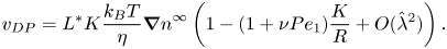
Anderson & Prieve (Reference Anderson and Prieve1984) made a review of early theoretical and experimental works on this phenomenon. The study considers both an electrolyte and non-electrolyte solute, the latter being relevant to the present paper. Anderson & Prieve (Reference Anderson and Prieve1984) focus specifically on models that predict the diffusiophoretic velocity  $v_{DP}$. This velocity depends on the interaction potential between the moving particle and the solute, or between the moving particle and smaller colloids depending on the type of mixture. Such a potential will be noted hereafter in its dimensionless form as
  $\varPi _{ic}$. The early
  $v_{DP}$ model of Derjaguin et al. (Reference Derjaguin, Sidorenkov, Zubashchenkov and Kiseleva1947) expresses
  $v_{DP}$ as a function of
  $\varPi _{ic}$ and of the solute concentration gradient, written in compact form as
 \begin{equation} v_{DP}= L^*K\frac{k_B T}{\eta} {\boldsymbol{\nabla} n}^\infty. \end{equation}
In (2.1),  $k_B$ is the Boltzmann constant, T is temperature,
  $\eta$ is the fluid viscosity and
  ${\boldsymbol {\nabla } n}^\infty$ is the far-field solute concentration gradient. Furthermore, K (called the adsorption length) and
  $L^*$ are functionals of the solute–interface interaction potential, defined as
 $$\begin{gather} K = \int_0^\infty \left(\mathrm{e}^{-\varPi_{ic}} - 1 \right) \, \mathrm{d} y, \end{gather}$$
 $$\begin{gather}L^* = \frac{1}{K}\int_0^\infty y\left(\mathrm{e}^{-\varPi_{ic}} - 1 \right) \, \mathrm{d} y. \end{gather}$$
In this equation y is the coordinate measuring the distance from the interface to a point in the mixture domain.
Equation (2.1) highlights that phoretic motion is proportional to the far-field solute concentration gradient, and that it is independent of the particle shape and size. The latter feature comes from the infinitesimally thin layer assumption, which presumes that both the interfacial layer length  $\lambda$ and the adsorption length K are much smaller than the minimum radius of curvature
  $R_c$ of the particle (Anderson & Prieve Reference Anderson and Prieve1991). Another hypothesis underlying (2.1) is that solute transport by convection is negligible.
When the condition  $K/{R_c} \to 0$ is not met, a new expression can be derived, which relates the phoretic velocity of a spherical particle to its radius R. This expression is (Anderson & Prieve Reference Anderson and Prieve1984)
 \begin{equation} v_{DP}= L^*K\frac{k_B T}{\eta}{\boldsymbol{\nabla} n}^\infty \left(1-\frac{K}{R}+O(\hat{\lambda}^2)\right). \end{equation}
To derive (2.3), the solute transport equation is once again decoupled from the fluid momentum balance by neglecting convective transport. The velocity profile can then be obtained using a dimensionless Stokes streamfunction. The velocity (and, consequently, the streamfunction itself) is expanded in powers of  $\hat {\lambda }$, which is the ratio between the thickness of the interfacial layer and the radius R. Each term can then be solved separately.
If solute transport by convection is accounted for in the diffusive layer, solute mass balance is no longer decoupled from the velocity profile near the sphere. The phoretic velocity in this case depends on the diffusion coefficient D. This dependency is captured via two dimensionless numbers,
 $$\begin{gather} {{Pe}_1} = \frac{n_m L^* K k_B T}{D\eta}, \end{gather}$$
 $$\begin{gather}{{Pe}_2} = \frac{{\boldsymbol{\nabla} n}^\infty R L^* K k_B T}{D\eta}. \end{gather}$$
In (2.4a),  $n_m$ is the mean far-field solute concentration. For most real phoretic systems,
  ${{Pe}_2} \approx 0$ (Anderson & Prieve Reference Anderson and Prieve1984). In the case where
  ${{Pe}_1}$ is of order
  $O(1)$ or higher, one must consider that the coefficients in the expansion in powers of
  $\hat {\lambda }$ depend on
  ${{Pe}_1}$. This yields (Anderson & Prieve Reference Anderson and Prieve1984)
 \begin{equation} v_{DP}= L^*K\frac{k_B T}{\eta}{\boldsymbol{\nabla} n}^\infty \left(1-(1+\nu {{Pe}_1})\frac{K}{R}+O(\hat{\lambda}^2)\right). \end{equation}
Equation (2.5) is a first-order approximation with respect to  $K/R$ and
  $\hat {\lambda }$ in the limit
  ${L/K \to 0}$. Note that (2.3) can be obtained from (2.5) by setting
  ${{Pe}_1}=0$. The new term
  $\nu$ in (2.5) is yet another functional of the solute–interface interaction potential, given by
 \begin{equation} \nu = \frac{1}{L^* K^2}\int_0^\infty \,\mathrm{d} y \left[\int_y^\infty \left(\mathrm{e}^{-\varPi_{ic}} - 1\right) \, \mathrm{d} y^* \right]^2, \end{equation}
where y and  $y^*$ represent the distance between a point in the domain and the surface of the sphere.
Anderson & Prieve (Reference Anderson and Prieve1991) generalized (2.5) for arbitrary  $K/R$. This equation is given by
 \begin{equation} v_{DP}= L^*K\frac{k_B T}{\eta}{\boldsymbol{\nabla} n}^\infty \left(1+(1+\nu {{Pe}_1})\frac{K}{R}\right)^{{-}1}. \end{equation}
Equation (2.7) still ignores solute transport via convection outside the diffusive layer (in the bulk), and it is valid in the limit  $\hat {\lambda } \to 0$ and
  $\lambda /K \to 0$.
The discussion in Anderson & Prieve (Reference Anderson and Prieve1984, Reference Anderson and Prieve1991) focuses on an adsorbing solute. This choice of solute–interface attractive-only interaction affects the validity of the simplifying assumptions (e.g.  $\lambda /K \to 0$), which in general hold true for adsorption. Note that for purely repulsive solute–interface interactions,
  $\varPi _{ic}>0$ and, hence, (2.2a) yields
  $|K|<\lambda$, so that
  $\lambda /K \to 0$ does not hold.
Keh & Weng (Reference Keh and Weng2001) improved on the previous works by finding an expression for the phoretic velocity that accounts for convective transport in the bulk, and without the restrictions  $\lambda /K \to 0$ and
  ${{Pe}_2} = 0$. The derivation follows closely that used by Anderson & Prieve (Reference Anderson and Prieve1991) to obtain (2.7). The frame of reference is set at the centre of the spherical particle, and the solute–interface interaction range
  $\lambda$ is again assumed small relative to the radius of the particle. With these considerations, the boundary layer approach can be used. It consists in solving the transport equations in the bulk (where the solute–interface interactions are negligible), and using a matching procedure to ensure the continuity of the solution at the surface of the sphere. Because
  $\lambda \ll R$, the boundary conditions (BCs) for the bulk transport equations can be imposed at
  $y=0$ instead of
  $y=\lambda$.
Furthermore, Keh & Weng (Reference Keh and Weng2001) claim that under the quasi-steady state assumption  $\partial n / \partial t$ (the time derivative of solute concentration) can be replaced by
  ${\boldsymbol {\nabla } n}^\infty v_{DP}$ in the solute transport equation for the bulk phase. Finally, the velocity and concentration profiles are expanded in powers of
  ${{Pe}_2}$, and matching between the inner (diffusive layer) and outer (bulk) profiles yields (Keh & Weng Reference Keh and Weng2001)
 \begin{equation} v_{DP}= L^*K\frac{k_B T}{\eta}{\boldsymbol{\nabla} n}^\infty \left(1+\beta\right)^{{-}1}\left(1+\alpha_2 {{Pe}_2}^2+O({{Pe}_2}^4)\right), \end{equation}
with
 $$\begin{gather} \beta = (1+\nu{{Pe}_1})\frac{K}{R}, \end{gather}$$
 $$\begin{gather}\alpha_2 ={-}\frac{\left(77+111\beta+274\beta^2+312\beta^3\right)(1+\beta)}{360\left(1+\beta^4\right)(1+2\beta)}. \end{gather}$$
 Note that the multiplying term before the brackets in (2.8) is the expression reported in (2.1). As a reminder, the latter is valid when convective transport is negligible, and when the curvature of the phoretic particle is much larger than the length of solute–interface interactions. In addition, one can see that (2.8) reduces to (2.7) when  ${{Pe}_2}=0$. Therefore, the former seems to be a more general version of the latter. However, there might be some issues with (2.8) and its derivation, which shall be discussed later in § 6.
Khair (Reference Khair2013) built on the work by Keh & Weng (Reference Keh and Weng2001) by studying the effect of solute advection on the motion of two phoretic particles. The strength of advection is measured via a third Péclet number  ${{Pe}_3}=b{\boldsymbol {\nabla } n}^\infty R/D$, with b being the mobility of the diffusive layer. In the absence of solute advection, the particles do not influence each other's motion, each translating as if it was isolated. However, if solute transport via convection is considered, the particles influence each other's movement, even for small
  ${{Pe}_3}$. A consequence of such a behaviour is that a pair of particles will tend to orient itself normal to the solute concentration gradient imposed. The time scale for this phenomenon depends on
  ${{Pe}_3}$: the higher
  ${{Pe}_3}$ is, the lower is the time required for particle orientation.
Assuming only that convection does not affect solute transport, Marbach et al. (Reference Marbach, Yoshida and Bocquet2020) found semi-analytical solutions for the diffusiophoretic velocity, when the particle is at mechanical equilibrium. Considering a potential  $\varPi _{ic}$ that depends only on the distance to the particle's surface, and also considering a constant solute gradient
  ${\boldsymbol {\nabla } n}^\infty$ far from the particle, the solute concentration profile in spherical coordinates is
 \begin{gather} n=n_0(r) + R {\boldsymbol{\nabla} n}^\infty \cos (\theta) f(r), \end{gather}
 \begin{gather} n_0(r) = n_m \mathrm{e}^{-\varPi_{ic}} \end{gather}
for  $f(r)$ such that
 \begin{equation} f(r): 2rf^\prime+r^2f^{\prime\prime}-2f+2r\varPi_{ic}^\prime f + r^2f^\prime \varPi_{ic}^\prime + r^2f\varPi_{ic}^{\prime\prime}=0. \end{equation}
In (2.10) and (2.11),  $\theta$ is the polar angle, R is the radius of the particle, r is the radial distance,
  $n_m=\lim _{r\to \infty }n(r,\theta ={\rm \pi} /2)$, and we consider that the solute concentration gradient far from the sphere is parallel to the azimuthal direction (
 $\theta =0$). The function
  $f(r)$ in (2.10) is defined by (2.12), where the superscript (
 $\prime$) indicates the derivative with respect to r. Note that there is no general solution for this differential equation. Nevertheless, one can still derive an expression for the diffusiophoresis velocity of the particle in terms of f (Marbach et al. Reference Marbach, Yoshida and Bocquet2020),
 \begin{equation} v_{DP}=\frac{R^2}{3\eta}{\boldsymbol{\nabla} n}^\infty k_B T \int_R^\infty f(r)(-\varPi_{ic}^\prime) \left(\frac{r}{R}-\frac{R}{3r}-\frac{2r^2}{3R^2} \right) \, \mathrm{d}r. \end{equation}
Equation (2.10) corresponds to an unnumbered equation in the first paragraph of § 3 in Marbach et al. (Reference Marbach, Yoshida and Bocquet2020). Equations (2.11) and (2.12) are not given in Marbach's paper, but they can be found by inserting (2.10) into the solute transport equation and later using the BCs to get rid of unknown constants. Finally, (2.13) is equation (3.23) in Marbach et al. (Reference Marbach, Yoshida and Bocquet2020).
Ramírez-Hinestrosa et al. (Reference Ramírez-Hinestrosa, Yoshida, Bocquet and Frenkel2020) studied the diffusiophoresis of a polymer in a mixture via molecular dynamic simulations. The interactions between the various particles in the system (monomers, solute and solvent molecules) were modelled with the 12-6 Lennard–Jones potential, except for monomer–monomer interactions. The authors found that the corresponding diffusiophoretic velocity depends weakly on the size of the polymer. Besides, it was shown that the effect of solute–monomer dispersion energy ( $\epsilon _{ms}$) on the mobility of the particle is non-monotonic. Mobility, defined as the ratio between diffusiophoretic velocity and the solute chemical potential gradient, is negative when monomers have more affinity with solvent molecules than solute molecules (i.e.
  $\epsilon _{ms}<1$). In other words, the polymer moves towards lower solute concentration regions when it has lower affinity with solute particles. When
  $\epsilon _{ms}>1$, the solute molecules are adsorbed around the polymer, and the direction of particle displacement is inverted. The mobility of the polymer continues to increase with respect to
  $\epsilon _{ms}$ until a certain threshold, after which it decreases, possibly due to the immobilization of the diffusive layer surrounding the polymer.
Finally, Popescu, Uspal & Dietrich (Reference Popescu, Uspal and Dietrich2016) made a concise review of self-diffusiophoresis, the phenomenon upon which an immersed particle itself creates the gradient of solute serving as the driving force for its motion. One of the mechanisms through which the particle can create this gradient is if its surface catalyses the formation/degradation of solute. A degree of asymmetry (e.g. anisotropic chemical activity over the surface) is necessary for motion to take place. Still in the context of self-diffusiophoresis, Michelin & Lauga (Reference Michelin and Lauga2014) proposed a framework for finding the phoretic velocity of Janus particles, i.e. particles whose surfaces have two or more distinct physical properties. Using this framework, the authors found that advection affects self-phoresis in a non-monotonic way: a maximum in phoretic velocity was found in their study for Péclet numbers of O(1).
3. Case study
The system used to study diffusiophoresis is depicted in figure 1. It consists of a spherical particle (black sphere) immersed in a mixture of solute (red circles) and water. The solute concentration gradient is kept constant very far from the sphere. The particle is assumed to be impermeable to solute and solvent alike, and a no-slip condition is imposed for the fluid at the particle's wall.
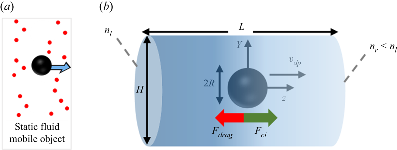
Figure 1. Diffusiophoresis set-up: spherical particle moving under the influence of a solute concentration gradient, when solute molecules repel the particle.
This set-up is axisymmetric with respect to the  $z$ axis passing through the centre of the sphere and parallel to the solute gradient. Therefore, instead of choosing a volume containing the sphere as the simulation box, one can simply choose a plane passing through the symmetry axis as the domain. In our simulations, we chose a rectangular simulation domain on the
  $Y$–
$Y$– $z$ plane, which translates into a cylindrical three-dimensional domain because of the rotational symmetry. The origin of the coordinate system is set at the centre of the cylinder, and as an initial condition, we place the centre of the sphere at the origin. The sphere may or may not move away from the centre of the cylinder, depending on the model used for simulation. The cylinder in this figure corresponds to the simulation domain, and its size can be arbitrarily chosen as long as
  $H,L\gg R$. A solute gradient
  ${\boldsymbol {\nabla } n}^\infty =(n_r-n_l)/L$ is imposed by fixing the solute concentration (number of particles per volume of mixture) at
  $z=-L/2$ (
 $n_l$) and at
  $z=L/2$ (
 $n_r$). Values of parameters used for simulations are given in table 1.
Table 1. Range of dimensions and parameters used for simulations.
In this table,  $n_m$ is the mean value of the far-field profile, given by
  $n_m=(n_l+n_r )/2$. Further, D is the diffusion coefficient of the solute forming the concentration gradient,
  $\eta$ is the fluid (water) viscosity and T is the temperature of the mixture. Finally,
  $k_{ic}$,
  $l_{ic}$ and
  $a_{tt}$ are parameters for the interface–solute interaction potential, as given in (4.4).
The spherical particle is subjected to the force exerted by the solute on its interface ( $F_{ci}$), and to the viscous drag
  $F_{drag}$ opposing particle motion. The direction of these forces depends on the nature of solute–interface interactions. If repulsive interactions dominate, the left-hand side of the domain (richer in solute) ‘pushes harder’ than the right-hand side, so
  $F_{ci}$ is positive and the drag force is negative. Alternatively, if attractive interactions dominate, the left part of the mixture ‘pulls harder’ than the right part, and the forces will be oriented oppositely.
The case study depicted in figure 1 is used to calculate diffusiophoretic velocities  $v_{DP}$ for several combinations of the parameters listed in table 1. The goal of these simulations is to regress an expression for
  $v_{DP}$. Furthermore, dynamic simulations of the case study in figure 1 shall show whether there exist fully developed states for which velocity and solute concentration profiles change with respect to time, but no longer depend on the initial conditions of the system. The last goal to be achieved through this case study is to investigate the influence of solute–interface attraction strength on diffusiophoresis.
4. Physical model
Classically, the modelling of solution flow is done assuming that the solute is sufficiently diluted so that its effect on the solvent flow can be neglected. However, in the case where interface–solute forces are present, these are transmitted to the fluid, for example, via viscous drag (Oster & Peskin Reference Oster and Peskin1992). The resultant body force on the solvent enters the Navier–Stokes equation as the gradient of an interaction potential, times the solute concentration. Furthermore, the action of the interface on the solute is accounted for via an extra convection term in the solute mass balance equation. The modified set of transport equations is then (Michelin & Lauga Reference Michelin and Lauga2014; Popescu et al. Reference Popescu, Uspal and Dietrich2016; Marbach et al. Reference Marbach, Yoshida and Bocquet2020)
 \begin{gather} \boldsymbol{\nabla}\boldsymbol{\cdot}\boldsymbol{u} = 0, \end{gather}
 \begin{gather} \eta \nabla^2\boldsymbol{u}-\boldsymbol{\nabla} p - k_BTn\boldsymbol{\nabla} \varPi_{ic}=\boldsymbol{0}, \end{gather}
 \begin{gather} \frac{\partial n}{\partial t}={-}\boldsymbol{\nabla}\boldsymbol{\cdot}\boldsymbol{J_n}={-}\boldsymbol{\nabla}\boldsymbol{\cdot}({-}D\boldsymbol{\nabla} n - Dn\boldsymbol{\nabla} \varPi_{ic} + n\boldsymbol{u}). \end{gather}
In these equations,  $\boldsymbol {u}$ stands for the velocity of the fluid, p is pressure,
  $\boldsymbol {J_n}$ is the solute flux and t is time. In addition,
  $-k_B T n \boldsymbol {\nabla } \varPi _{ic}$ is the body force that is transmitted from the solute to the solvent, with
  $k_B$ being the Boltzmann constant and
  $\varPi _{ic}$ being the interface–solute interaction potential. Note that (4.1) assumes an incompressible fluid, whereas (4.2) neglects inertia.
There are several ways to model the solute–interface interaction potential. For steric exclusion,  $\varPi _{ic}=+\infty$ for
  $y\leq a$ and
  $\varPi _{ic}=0$ for
  $y>a$, with a being the size of the solute species and y being the distance between the interface and a point in the domain. For charged particles with an electric double layer in a mixture with polar solute molecules,
  $\varPi _{ic}$ depends on the local electric field and on the dipole moment of the solute (Anderson Reference Anderson1989). In the present work
  $\varPi _{ic}$ is modelled as the sum of a repulsive and an attractive exponential term, as proposed by Bacchin (Reference Bacchin2017),
 \begin{equation}
\varPi_{ic}=k_{ic}\left[\overbrace{(1+a_{tt})\mathrm{e}^{-({y}/
{l_{ic}})}}^{\textrm{repulsion}}-
\overbrace{a_{tt}\mathrm{e}^{-({y}/{2l_{ic}})}}^{\textrm{attraction}}\right].
\end{equation}
\begin{equation}
\varPi_{ic}=k_{ic}\left[\overbrace{(1+a_{tt})\mathrm{e}^{-({y}/
{l_{ic}})}}^{\textrm{repulsion}}-
\overbrace{a_{tt}\mathrm{e}^{-({y}/{2l_{ic}})}}^{\textrm{attraction}}\right].
\end{equation}
In (4.4) the parameter  $a_{tt}$ can be used to depict pure repulsion (
 $a_{tt}=0$) and long-range attraction with short-range repulsion (
 $a_{tt}>0$) to keep physical consistency with volume exclusion. Term
  $k_{ic}$ represents the magnitude of interface–solute interactions, y is the distance between the interface and a point in the domain and
  $l_{ic}$ is the interaction range. The repulsion term in
  $\varPi _{ic}$ is similar to the negative exponential function used in DLVO (Derjaguin–Landau–Verwey–Overbeek) theory to model repulsion between electric double layers (Bhattacharjee, Elimelech & Borkovec Reference Bhattacharjee, Elimelech and Borkovec1998). Because an exponential decay is a stiff function, this repulsion term may also model steric exclusion if
  $l_{ic}$ is of the same order of magnitude as the solute particle's size. Furthermore, the attraction term may account for solute adsorption near the solid walls (Bacchin, Glavatskiy & Gerbaud Reference Bacchin, Glavatskiy and Gerbaud2019). The factor 1/2 in the power of the second exponential distinguishes the range of attractive interactions from the range of repulsive interactions. In (4.4) the range of attraction (
 $2l_{ic}$) is longer than the range of repulsion (
 $l_{ic}$).
In the next subsections, three options are discussed to model the diffusiophoretic system depicted in figure 1, based on (4.1)–(4.3). They may be chosen depending on the reference frame (the lab or the phoretic particle), and on whether or not convection can be neglected in (4.3). Simulation results from these models are shown later in § 6, along with the main conclusions drawn from them.
4.1. Transient exact formulation
The transient exact formulation (TEF) model uses the laboratory reference frame. In this frame of reference the fluid far from the particle is considered stagnant. The particle is therefore moving, and its velocity is a BC for the fluid on the fluid–particle interface. Furthermore, it is common to assume that the solute profile is well-established far from the particle, and that the latter moves under the influence of a distant solute gradient  $\boldsymbol {\nabla } n^\infty$ (Anderson & Prieve Reference Anderson and Prieve1984, Reference Anderson and Prieve1991; Churaev et al. Reference Churaev, Derjaguin and Muller1987; Anderson Reference Anderson1989; Khair Reference Khair2013; Marbach et al. Reference Marbach, Yoshida and Bocquet2020; Ramírez-Hinestrosa et al. Reference Ramírez-Hinestrosa, Yoshida, Bocquet and Frenkel2020; Rasmussen, Pedersen & Marie Reference Rasmussen, Pedersen and Marie2020). The BCs for (4.1)–(4.3) are then listed as six equalities, i.e.
 $$\begin{gather} \boldsymbol{u}|_{{interface}(t)} = \boldsymbol{v_0}, \end{gather}$$
 $$\begin{gather}\boldsymbol{u}|_\infty = \boldsymbol{0}, \end{gather}$$
 $$\begin{gather}\frac{\mathrm{d}\boldsymbol{v_0}}{\mathrm{d}t} = \frac{\boldsymbol{F}}{M}, \end{gather}$$
 $$\begin{gather}(\boldsymbol{J_n}-\boldsymbol{v_0}n)\boldsymbol{\cdot}\boldsymbol{e}|_{{interface}(t)} = 0, \end{gather}$$
 $$\begin{gather}n|_{t=0} = n_0(\boldsymbol{x}), \end{gather}$$
 $$\begin{gather}n|_{r\to\infty} = n^\infty(\boldsymbol{x}), \end{gather}$$
where the force  $\boldsymbol {F}$ acting on the particle can be calculated by
 \begin{equation} \boldsymbol{F} = \int_\varOmega k_B T n \boldsymbol{\nabla}\varPi_{ic} \, \mathrm{d}V + \int_{\partial\varOmega}\eta \left(\boldsymbol{\nabla}\boldsymbol{u} + {\boldsymbol{\nabla}\boldsymbol{u}}^\mathrm{T} \right)\boldsymbol{\cdot}\boldsymbol{e} \, \mathrm{d}S - \int_{\partial\varOmega} p\boldsymbol{e} \, \mathrm{d}S \end{equation}
 Equality (4.5a) corresponds to the no-slip condition; subscript interface (t) refers to the moving (time-dependent) surface of the particle and  $v_0$ refers to its velocity. Equality (4.5b) means that the fluid is at rest far from the particle. Equality (4.5c) is Newton's second law applied to the particle, where
  $M$ is the mass of the particle. Equation (4.5d) guarantees that solute molecules cannot enter the particle (
 $\boldsymbol {e}$ is the unit vector normal to the particle's surface). The BC in (4.5e) represents the initial condition of the solute concentration profile. Finally, the last BC (4.5 f) stresses that the solute concentration profile is not perturbed far from the particle. The distance r on the left-hand side is the distance from the centre of the spherical particle. Because the gradient of solute far from the particle is considered constant,
  $n^\infty$ depends on the position
  $\boldsymbol {x}$. It is a linear concentration profile.
Equations (4.1)–(4.3) with the BCs given by (4.5) define the dynamics of diffusiophoresis. According to (4.6), the particle is subjected to the action of three forces, namely a solute–interface interaction force (first term) and hydrodynamic forces due to viscous stress (second term) and due to pressure (third term). The volumetric integral is taken over the entire domain, whereas the surface integrals are taken over the particle's surface. One is often interested in the equilibrium state, for which  $\boldsymbol {F}=\boldsymbol {0}$. Indeed, because the inertia of the particle is often negligible, it accelerates so fast that the drag quickly becomes equal to the force exerted on the sphere by the solute. However, neglecting the inertia of the particle would complicate the TEF simulations, because at every time step a number of iterations would be required until the equilibrium velocity is found. At the same time, considering a sphere density of
  $1000\,{\rm kg}\,{\rm m}^{-3}$ for instance would require very small time steps to avoid unrealistically high particle velocities in the first few time iterations. With such small time steps, capturing the effect of particle displacement and solute transport is impractical. To avoid these issues, the sphere density considered in the TEF simulations was set to be much higher (by a factor of
  $10^4$) than the density of water. This is simply a mathematical artifice to facilitate the simulations.
The transient formulation presented above has many interesting applications. One of them is answering whether the solution of (4.1)–(4.3) and (4.5) depends on the initial conditions as the time goes to infinity. This topic is addressed in § 6.1. In addition, TEF simulations can be used to illustrate particle separation (§ 6.2).
4.2. Transient formulation at constant velocity (TFCV)
Equations (4.1)–(4.3) and (4.5), (4.6) are the exact description of the case study. However, such a model has a high computation cost, since the problem is transient and the domain needs to be remeshed at every time step. To avoid remeshing, one can assume that the velocity  $\boldsymbol {v_0}$ of the particle is constant. The origin can then be set at the centre of the particle by defining new coordinates
  $\boldsymbol {x}=\boldsymbol {x}^*-\boldsymbol {v_0}t$, where
  $\boldsymbol {x}^*$ are the coordinates in the rigid frame. In this new moving frame, it is suitable to define a new variable
  $\boldsymbol {w}=\boldsymbol {u}-\boldsymbol {v_0}$ corresponding to the relative velocity of the fluid with respect to the sphere. In this case, (4.1)–(4.3) and (4.5) can be rewritten as (Brady Reference Brady2011)
 \begin{gather} \boldsymbol{\nabla}\boldsymbol{\cdot}\boldsymbol{w} = 0, \end{gather}
 \begin{gather} \eta{\boldsymbol{\nabla}}^2\boldsymbol{w}-\boldsymbol{\nabla} p - k_B T n \, \boldsymbol{\nabla} \varPi_{ic}=\boldsymbol{0}, \end{gather}
 \begin{gather} -\boldsymbol{\nabla}\boldsymbol{\cdot}\boldsymbol{J_n}={-}\boldsymbol{\nabla}\boldsymbol{\cdot}({-}D\boldsymbol{\nabla} n - D n \, \boldsymbol{\nabla} \varPi_{ic} + n \boldsymbol{w})=\frac{\partial n}{\partial t}, \end{gather}
 $$\begin{gather} \boldsymbol{w}|_{interface} = \boldsymbol{0}, \end{gather}$$
 $$\begin{gather}\boldsymbol{w}|_\infty ={-}\boldsymbol{v_0}, \end{gather}$$
 $$\begin{gather}\boldsymbol{J_n}\boldsymbol{\cdot}\boldsymbol{e}|_{interface} = 0, \end{gather}$$
 $$\begin{gather}n|_{t=0} = n_0(\boldsymbol{x}), \end{gather}$$
 $$\begin{gather}n|_{r\to\infty} = n^\infty(\boldsymbol{x}) + {\boldsymbol{\nabla} n}|_\infty \boldsymbol{\cdot} \boldsymbol{v_0} \, t. \end{gather}$$
 The term  $\boldsymbol {J_n}$ corresponds to the solute flux perceived by the particle. Equations (4.7)–(4.10) can be simulated using a fixed mesh. The translation of the particle is captured by the transient BC given in (4.10e). However, this set of equations is not equivalent to the dynamic formulation described previously, because here we assume constant particle velocity. Despite that, this formulation can capture instantaneous equilibrium states. That is, for a given
  $\boldsymbol {v_0}$, one can run a simulation with (4.7)–(4.10) and check if the force
  $\boldsymbol {F}$ acting on the particle equals zero at some time t. It is also possible to distinguish whether a certain equilibrium state is momentary or persistent. Indeed, if a simulation using this formulation shows that the force acting on the surface remains very close to 0 during a large time interval, that means the actual dynamic system will also sustain an equilibrium state during the same interval.
4.3. High diffusion limit
In the limit of very high diffusion coefficients ( $D\to \infty$), convective solute transport and the transient term
  $\partial n / \partial t$ in the solute transport equation can be neglected. The equations describing this formulation are
 \begin{gather} \boldsymbol{\nabla}\boldsymbol{\cdot}\boldsymbol{w} = 0, \end{gather}
 \begin{gather} \eta{\boldsymbol{\nabla}}^2\boldsymbol{w}-\boldsymbol{\nabla} p - k_B T n \, \boldsymbol{\nabla} \varPi_{ic}=\boldsymbol{0}, \end{gather}
 \begin{gather} \boldsymbol{\nabla}\boldsymbol{\cdot}\boldsymbol{J_n} = \boldsymbol{\nabla}\boldsymbol{\cdot}({-}D\boldsymbol{\nabla} n - D n \, \boldsymbol{\nabla} \varPi_{ic}) = 0, \end{gather}
 $$\begin{gather} \boldsymbol{w}|_{interface} = \boldsymbol{0}, \end{gather}$$
 $$\begin{gather}\boldsymbol{w}|_\infty ={-}\boldsymbol{v_0}, \end{gather}$$
 $$\begin{gather}\boldsymbol{J_n}\boldsymbol{\cdot}\boldsymbol{e}|_{interface} = 0, \end{gather}$$
 $$\begin{gather}n|_{r\to\infty} = n^\infty(\boldsymbol{x}). \end{gather}$$
These equations are in the frame of reference of the particle, which is why the velocity is set to zero on the particle's surface in (4.14a).
The high diffusion limit (HDL) formulation is commonly used in the literature (Sharifi-Mood, Koplik & Maldarelli Reference Sharifi-Mood, Koplik and Maldarelli2013; Popescu et al. Reference Popescu, Uspal and Dietrich2016; Marbach et al. Reference Marbach, Yoshida and Bocquet2020), mainly because it decouples the solute transport equation from the momentum balance of the mixture. In other words, one can solve (4.13) to find the solute concentration profile (2.10) before computing the velocity and pressure fields. In addition, HDL does not require time iterations: the velocity and solute concentration profiles are established instantaneously for any given far-field BC  $n^\infty (\boldsymbol {x})$. The semi-analytical expression for the phoretic velocity from the HDL formulation is given in (2.13).
5. Numerical simulation set-up and validation
In this work the ANSYS Fluent $^\circledR$ software (Ansys Inc 2020) is chosen to perform diffusiophoresis simulations, with help of the coupled algorithm (Ansys Inc 2021) solver that solves the momentum and continuity equations simultaneously. The software supports dynamic meshing, which is a required feature to implement the TEF model described in § 4.1. Typically, the computation time for one transient simulation remains within less than 24 h for a large number of time steps (up to 400) and refined mesh (up to
  $1.3\times 10^6$ elements) using four processors.
To implement the equations, we use the laminar model available in Fluent to simulate fluid flow, and define a user-defined scalar to describe solute transport (Ansys Inc 2021). The extra term  $-k_B T n \, \boldsymbol {\nabla }\varPi _{ic}$ appearing in the momentum balance equation for the fluid, which corresponds to the force exerted by the interface on the solute (transferred to the solvent), is handled via a source term. Furthermore, the additional term
  $-D n \, \boldsymbol {\nabla }\varPi _{ic}$ in the solute transport equation, which represents the transport due to interface–solute forces, is captured via a user-defined function (UDF). User-defined functions are also necessary to prescribe the motion of the sphere in the TEF model. More details on these UDFs are given in the supplementary material available at https://doi.org/10.1017/jfm.2022.1067.
The ranges of solute concentration  $n_m$ and far-field solute concentration gradient
  ${\boldsymbol {\nabla } n}^\infty$ used to define the far-field solute concentration profile are shown in table 1. For the TEF model, the velocity at the left and right boundaries is set to 0 as the fluid far from the sphere is considered at rest. Furthermore, no-slip BC is imposed at the wall, whose velocity is updated based on the forces exerted on the sphere. The solute concentration values at the left and right boundaries are calculated from
  $n_m$ and
  ${\boldsymbol {\nabla } n}^\infty$. On the other hand, both TFCV and HDL models place the sphere at the origin of the reference frame. Therefore, null velocity is imposed for the fluid on the surface of the sphere. The velocity at the left and right boundaries is imposed, and it is kept the same throughout the simulation. The initial concentrations at the left and right boundaries are calculated from
  $n_m$ and
  ${\boldsymbol {\nabla } n}^\infty$, but they are updated for the TFCV model according to (4.10e). Finally, in the three diffusiophoretic models, an axis-symmetry BC is imposed on the axial axis passing through the centre of the sphere, a symmetry BC is imposed on the shell of the cylindrical domain in figure 1 and a zero solute flux is imposed on the walls of the sphere.
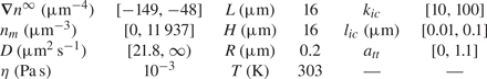
The mesh used in all diffusiophoresis simulations is shown in figure 2. It consists of a structured zone with regular squared elements far from the sphere, an inflation layer around the sphere and an unstructured mesh region between these zones. The total number of elements is 1 317 824, and the maximum element size is set to  $0.01\,{\mathrm {\mu }{\rm m}}$ (5 % of the radius of the sphere). The different mesh zones are clearer in the right extract of figure 2, which zooms in a small portion of the domain around the sphere. When the entire domain is displayed (left image), the elements are not visible and the entire mesh has a solid dark aspect, due to the limited pixel resolution.
Figure 2. Mesh used for the diffusiophoresis case study.
This mesh was validated by comparing simulation results between meshes with a maximum element size either equal to  $0.01\,\mathrm {\mu }{\rm m}$ or
  $0.016\,\mathrm {\mu }{\rm m}$. Figure 3 shows the comparison of the axial velocity profiles for both meshes, using the TFCV model with
  ${\boldsymbol {\nabla } n}^\infty =-149 \, \mathrm {\mu }{\rm m}^{-4}$,
  $n_m=1193.7 \, \mathrm {\mu }{\rm m}^{-3}$,
  $D = 218 \, \mathrm {\mu }{\rm m}^2\,{\rm s}^{-1}$, and setting the velocity at the inlet and outlet to zero. Note that the deviation between these profiles is negligible compared with the absolute range of variation in velocity (
 ${\approx }47.3 \, \mathrm {\mu }{\rm m}\,{\rm s}^{-1}$). A second type of validation was performed by slightly displacing the sphere from the centre of the domain, while keeping the same
  $n_m$. It was found that this modification could change the calculated diffusiophoretic velocities significantly, especially when drag and solute–sphere interaction forces are of the order of
  $10^{-14} \, {\rm N}$ or lower. However, this discrepancy vanishes if the inflation layer is at least four times thicker than the radius of the sphere. This condition was taken into account in the mesh shown in figure 2.
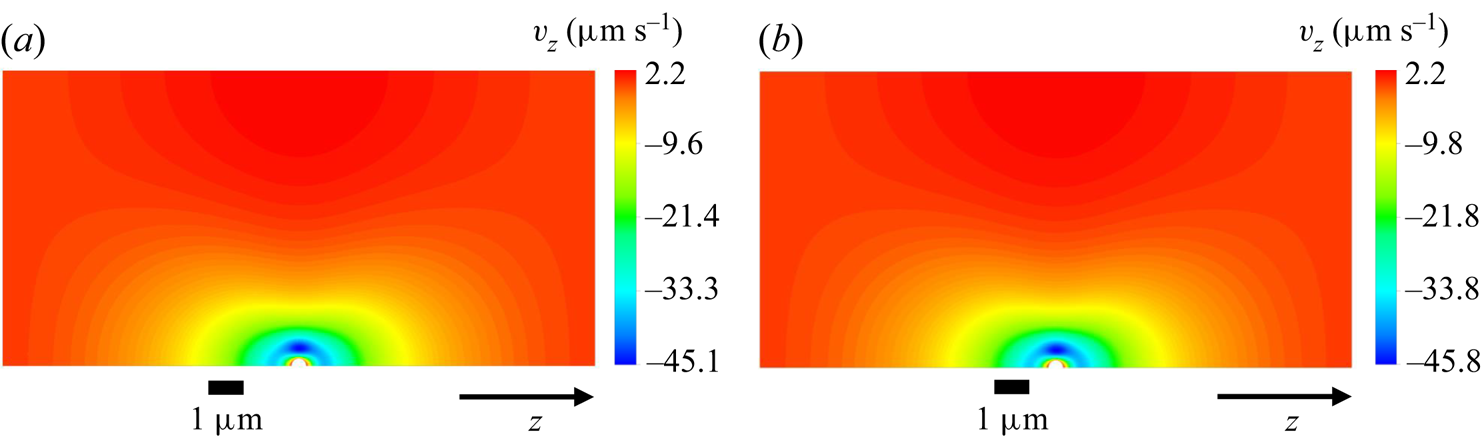
Figure 3. Comparison of axial velocity profiles in the diffusiophoresis case study, using meshes with maximum element size of (a)  $0.01\,\mathrm {\mu }{\rm m}$ and (b)
  $0.016\,\mathrm {\mu }{\rm m}$.
A third kind of mesh validation was performed by comparing simulation results with analytical results of Marbach et al. (Reference Marbach, Yoshida and Bocquet2020). The authors derived a semi-analytical expression for the diffusiophoretic velocity in the HDL model, given by (2.12) and (2.13). Note that the differential equation (2.12) does not have a general explicit solution. However, a careful study of these equations led to the finding of a specific interface–solute interaction potential  $\varPi _{ic}$ that results in a fully analytical expression for diffusiophoretic velocity. Such a mathematically convenient
  $\varPi _{ic}$ is given by (5.1), and the corresponding analytical solutions for (2.12) and (2.13) are given in (5.2) and (5.3) as follows:
 \begin{gather} \varPi_{ic}=\frac{1}{2}\ln{\left(\frac{r^4}{r^4+R^4}\right)}, \end{gather}
 \begin{gather} f(r)=\frac{r}{R}+\frac{R^3}{r^3}, \end{gather}
 \begin{gather} v_{DP}=\frac{R^2}{6\eta}{\boldsymbol{\nabla} n}^\infty k_B T. \end{gather}
 The  $\varPi _{ic}$ potential in (5.1) does not have a physical significance. However, it works as a convenient mathematical artifice that can be used together with (5.3) to quickly assess numerical implementations of the HDL model presented in § 4.3. This has significant importance due to the relative popularity of the model in the literature (Sharifi-Mood et al. Reference Sharifi-Mood, Koplik and Maldarelli2013; Popescu et al. Reference Popescu, Uspal and Dietrich2016; Marbach et al. Reference Marbach, Yoshida and Bocquet2020).
For values of R,  $\eta$ and T given in table 1, and for
  ${\boldsymbol {\nabla } n}^\infty = -149 \, \mathrm {\mu }{\rm m}^{-4}$, one obtains a theoretical diffusiophoresis velocity
  $v_{DP} = -4.09 \, \mathrm {\mu }{\rm m}\,{\rm s}^{-1}$. From numerical simulation, the value obtained is
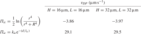
  $v_{DP} = -3.86 \, \mathrm {\mu }{\rm m}\,{\rm s}^{-1}$, corresponding to a relative error of 5.6 %. The source of the error is not the meshing itself, but rather the size of the simulation domain, which is too small for a logarithmic potential. Indeed, doubling H and L given in table 1 (without changing the mesh element size) results in a new simulated velocity of
  $-3.97 \, \mathrm {\mu }{\rm m}\,{\rm s}^{-1}$, and the error is reduced to 2.9 %. Nevertheless, we keep the values of H and L in table 1 for all simulations when the exponential potential in (4.4) is used, because in this case the variation of
  $v_{DP}$ with respect to domain size is much smaller. The reason for this difference is that the logarithmic potential in (5.1) decays in
  $1/r^4$, which makes it act over longer distances compared with a potential that decays exponentially. Table 2 summarizes the changes in
  $v_{DP}$ considering different domain sizes and interface–solute interaction potential. The results for the exponential potential considered
  ${\boldsymbol {\nabla } n}^\infty = -149 \, \mathrm {\mu }{\rm m}^{-4}$,
  $n_m = 4775 \, \mathrm {\mu }{\rm m}^{-3}$,
  $k_{ic}=100$,
  $l_{ic}=0.1 \, \mathrm {\mu }{\rm m}$ and
  $a_{tt}=0$.
Table 2. Comparison between  $v_{DP}$ calculated using different domain sizes.
This section validated the set-up for diffusiophoresis simulations by assessing the impact of mesh element size, mesh structure and simulation box size on the diffusiophoretic velocity and on the flow velocity profile. It was found that the mesh structure must have an inflation layer at least four times thicker than the radius of the sphere in order to avoid significant numerical errors. Furthermore, the size of the mesh elements and of the simulation domain were found to be adequate.
6. Results and discussion
This section discusses simulation results for the diffusiophoretic case study in § 3, obtained according to the models described in § 4.
6.1. Influence of initial conditions on long-time behaviour of the system
Transient flow simulation describes the motion of the particle in the solute gradient. As the particle moves along (or against) this gradient, the amplitude of the forces acting on it (drag and solute–interface forces) will change. Furthermore, because the force applied by solute molecules on the interface depends on the solute concentration profile around the sphere, the motion of the particle should depend on its initial position with respect to the solute gradient. Nevertheless, it is worth questioning whether the system ‘forgets’ its initial state after a large enough time. This is presented next with the help of the two transient model formulations TEF (§ 4.1) and TFCV (§ 4.2), which represent slightly different physical systems. The TEF corresponds to a particle set free in a stagnant solution with a concentration gradient. Its velocity changes according to the forces exerted on its surface, as indicated by (4.5c). On the other hand, TFCV assumes that particle velocity remains the same.
The question of whether the system ‘forgets’ its initial state after a large enough time can be translated as follows. Imagine two systems A and B under the same imposed far-field solute concentration gradient, each of them containing a spherical particle of radius R that occupy different positions at time  $t=0$. The position of these spheres can be tracked by the far-field solute concentration
  $n_m$, so the initial positions will be named
  $n_m^{A,0}$ and
  $n_m^{B,0}$. Without loss of generality, let us say these particles are moving right, and the sphere in system B starts ahead of the sphere in A. Eventually, these particles will pass through an arbitrary position
  $n_m^{\Delta }$, though they will not reach this position at the same time. Still, is it possible to distinguish one system from another when they are at position
  $n_m^{\Delta }$? Figure 4 illustrates the above discussion.
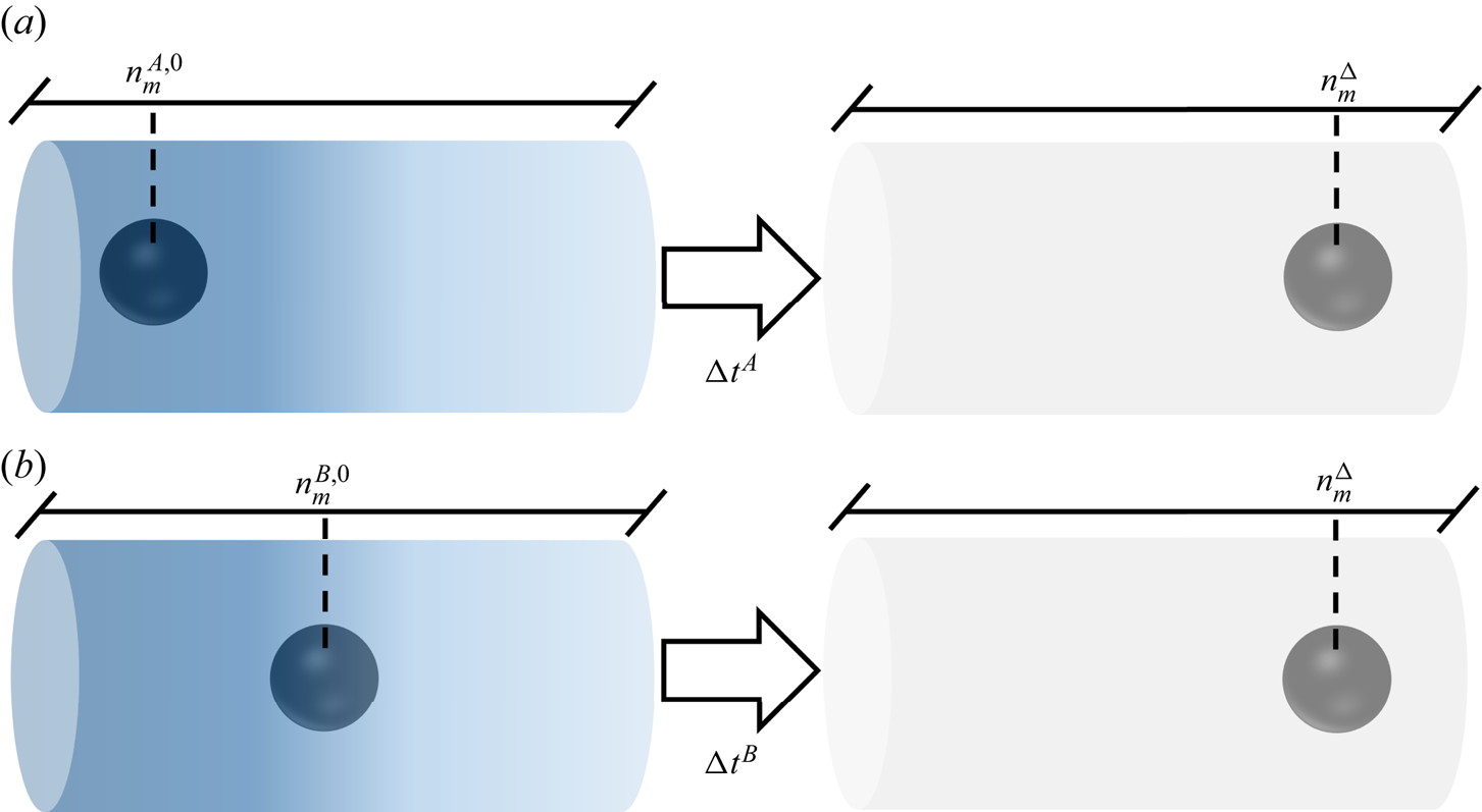
Figure 4. Illustration of the possible dependency of a diffusiophoretic system on initial conditions, with two particles moving under the same far-field solute concentration profile, but starting from different positions.
The formal mathematical statement for the question depicted in figure 4 is given as follows. If the profiles  $n^A(\boldsymbol {x},t)$,
  $\boldsymbol {u}^A(\boldsymbol {x},t)$ and
  $n^B(\boldsymbol {x},t)$,
  $\boldsymbol {u}^B(\boldsymbol {x},t)$ are solutions of (4.1)–(4.3) and (4.5), or (4.7) to (4.10), with the same BCs but with different initial conditions, then
 $$\begin{gather} \lim_{t\to\infty}[n^A(\boldsymbol{x},t+t^\prime)-n^B(\boldsymbol{x},t)] \stackrel{?}= 0, \end{gather}$$
 $$\begin{gather}\lim_{t\to\infty}[\boldsymbol{u}^A(\boldsymbol{x},t+t^\prime)-\boldsymbol{u}^B(\boldsymbol{x},t)] \stackrel{?}= \boldsymbol{0}, \end{gather}$$
where  $t^\prime$ is such that
 \begin{equation} n_m^A(t+t^\prime)=n_m^B(t). \end{equation}
If (6.1) is true, we can say that the system reaches a fully developed state. That does not mean its properties will not change with respect to time, but rather that they become independent of the initial state.
The complexity and nonlinearity of the PDE system describing diffusiophoresis prevents a rigorous mathematical approach to (6.1). However, numerical simulations can shed light on the validity of this equation. At first, one can investigate the evolutions of two systems A and B using the TFCV formulation described in § 4.2. Velocity  $\boldsymbol {v}_0$ in (4.10b) is set to
  $14.6\,\mathrm {\mu }{\rm m}\,{\rm s}^{-1}$. In addition, a diffusion coefficient of
  $21.8\,\mathrm {\mu }{\rm m}^2\,{\rm s}^{-1}$ is considered. Both systems are under a linear far-field solute concentration profile with
  ${\boldsymbol {\nabla } n}^\infty =-149 \, \mathrm {\mu }{\rm m}^{-4}$. Furthermore, particles start at different positions, with
  $n_m^{A,0}=1551.8 \, \mathrm {\mu }{\rm m}^{-3}$ and
  $n_m^{B,0}=1408.5 \, \mathrm {\mu }{\rm m}^{-3}$. The initial concentration profile
  $n_0(\boldsymbol {x})$ is linear in both systems, with
  $\boldsymbol {\nabla } n^A(\boldsymbol {x},0)=\boldsymbol {\nabla } n^B(\boldsymbol {x},0)={\boldsymbol {\nabla } n}^\infty \boldsymbol {e_z}$. Figure 5(a) shows how the forces in each system change with respect to the position
  $n_m$ of the particle. Figure 5(b,c) shows two other pairs A, B with different diffusion coefficients (respectively 218 and
  $2180\,\mathrm {\mu }{\rm m}^2\,{\rm s}^{-1}$) and particle velocities (80.9 and
  $200\,\mathrm {\mu }{\rm m}\,{\rm s}^{-1}$, respectively). All simulations were run with
  $k_{ic}=100$,
  $l_{ic}=0.1 \, \mathrm {\mu }{\rm m}$ and
  $a_{tt}=0$.
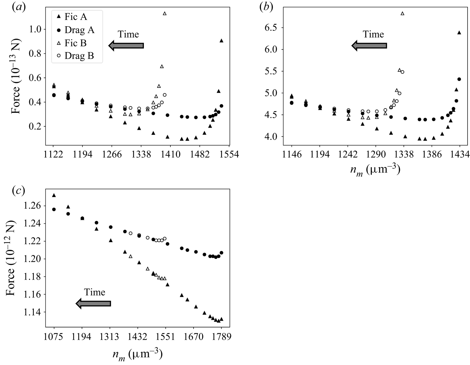
Figure 5. Solute–interface force (triangles) and minus drag force (circles) acting on the particle in different pairs of systems A and B, in transition to fully developed state according to TFCV predictions. Results are shown for (a)  $D=21.8 \, \mathrm {\mu }{\rm m}^2\,{\rm s}^{-1}$,
  $\boldsymbol {v_0}=14.6 \, \mathrm {\mu }{\rm m}\,{\rm s}^{-1}$; (b)
  $D=218 \, \mathrm {\mu }{\rm m}^2\,{\rm s}^{-1}$,
  $\boldsymbol {v_0}=80.9 \, \mathrm {\mu }{\rm m}\,{\rm s}^{-1}$; (c)
  $D=2180 \, \mathrm {\mu }{\rm m}^2\,{\rm s}^{-1}$,
  $\boldsymbol {v_0}=200 \, \mathrm {\mu }{\rm m}\,{\rm s}^{-1}$.
The time arrow shows the direction of the particle movement (towards lower solute concentrations). Note that in the range  $n_m\in (1410,1554)$, the plot in figure 5(a) only shows data for system A. This is because the particle in B starts at
  $n_m^{B,0}=1410$ and moves towards smaller values of
  $n_m$. Furthermore, all the systems displayed in figure 5 reach an equilibrium of forces
  $(|F_{drag}|=|F_{ic}|)$ when
  $n_m=1194 \, \mathrm {\mu }{\rm m}^{-3}$. This is not by accident: the velocity
  $\boldsymbol {v_0}$ for each system in figure 5 was carefully chosen so that the sphere in A is at equilibrium when
  $n_m=1194 \, \mathrm {\mu }{\rm m}^{-3}$.
It is clear that the forces in each pair A, B tend to the same values as  $n_m$ gets smaller (i.e. as
  $t\to \infty$). Such a result suggests that (6.1) is true, at least for the set of parameters used in these simulations. This conclusion is confirmed when comparing the concentration and velocity profiles for systems A and B in figure 5. For each pair, when
  $n_m=1194 \, \mathrm {\mu }{\rm m}^{-3}$, concentration and velocity profiles are identical everywhere, within numerical accuracy. This is illustrated in figure 6 for
  $D=218 \, \mathrm {\mu }{\rm m}^2\,{\rm s}^{-1}$ and
  $\boldsymbol {v_0}=80.9 \, \mathrm {\mu }{\rm m}\,{\rm s}^{-1}$.

Figure 6. Concentration and  $z$-velocity profiles corresponding to (a,b) system A and (c,d) system B in figure 5(b) at
  $n_m=1194 \, \mathrm {\mu }{\rm m}^{-3}$.
Results for the TEF model described in § 4.1 show a similar behaviour. Let us consider two systems A and B with the same BCs and initial velocity 0, but starting at different positions  $(n_m^{A,0}\neq n_m^{B,0})$. As the particles move away from their initial positions, the forces go rapidly to 0 because of the low inertia. The data corresponding to the beginning of the motion, when the particle is transitioning to this quasi-equilibrium state, are not accurate. This is because the simulations neglected fluid inertia while assuming an unrealistically high particle density. However, as explained in § 4.1, this is only a mathematical artifice to facilitate the numerical study. After this transitioning period, results show that the corresponding particle velocities tend to the same values. Furthermore, solute concentration and velocity profiles converge to the same values, indicating that (6.1) is valid in the TEF. Figure 7 illustrates this behaviour for one particular pair of systems, with
  $D=2180 \, \mathrm {\mu }{\rm m}^2\,{\rm s}^{-1}$,
  ${\boldsymbol {\nabla } n}^\infty =-149 \, \mathrm {\mu }{\rm m}^{-4}$,
  $k_{ic}=100$,
  $l_{ic}=0.1 \, \mathrm {\mu }{\rm m}$ and
  $a_{tt}=0$. The initial positions for A and B are
  $n_m^{A,0}=1552 \, \mathrm {\mu }{\rm m}^{-3}$ and
  $n_m^{B,0}=1456 \, \mathrm {\mu }{\rm m}^{-3}$.
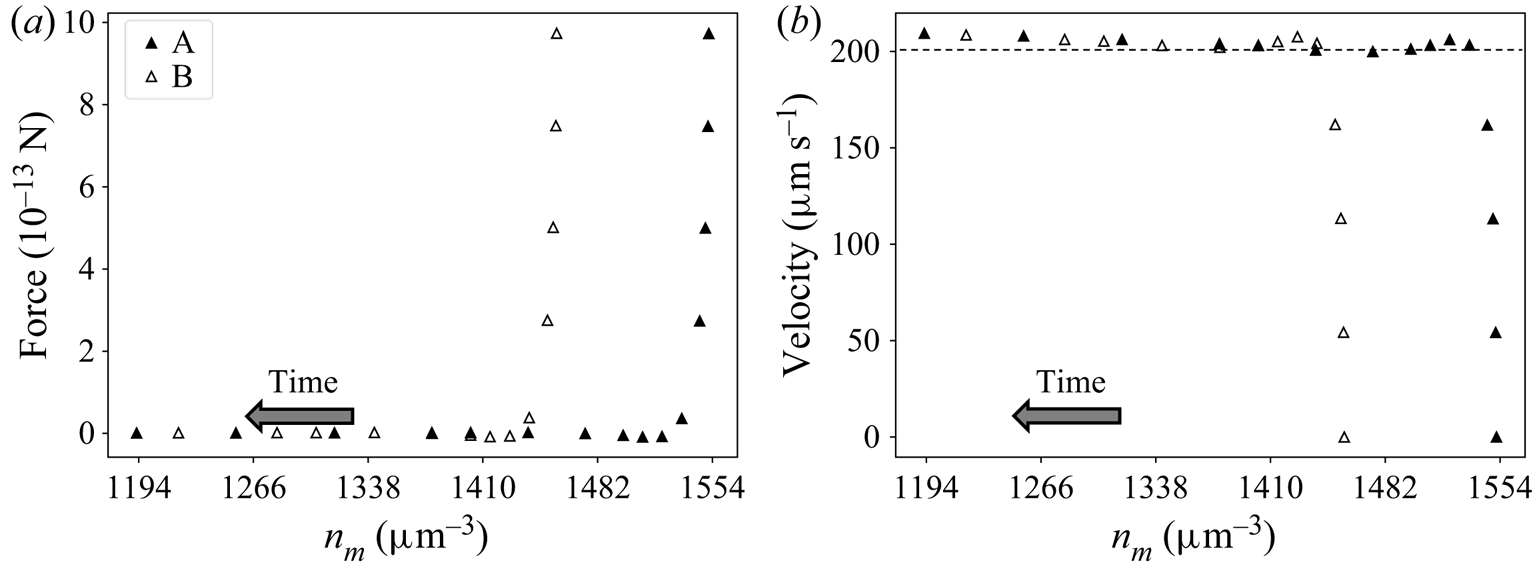
Figure 7. (a) Resultant force and (b) particle velocity for a pair of systems A, B in transition to a fully developed state according to TEF predictions; the dashed line corresponds to the diffusiophoretic velocity predicted by TFCV for  $n_m=1194 \, \mathrm {\mu }{\rm m}^{-3}$.
Figure 7(b) shows that the phoretic velocity does not reach a plateau. Instead, the particle continues to accelerate due to small differences between the solute–interface force and the drag force. This difference, depicted in figure 5 for the TFCV model, persists in time because the driving force exerted by the solute on the interface depends on the position of the sphere with respect to the solute concentration profile (i.e.  $n_m$). Hence, contrary to other phenomena like settling where the driving force is constant, it is generally not possible to reach a limiting velocity (with no acceleration) in diffusiophoresis. The only special case in which a limiting velocity can be reached is if such a velocity is 0; in this case, the particle remains stagnant in the mixture. Still, figure 7(b) shows that the equilibrium velocity predicted by the TFCV (dashed line) is close to the actual phoretic velocities obtained via TEF.
The force amplitude being dependent on the position, the movement of the sphere and the state of the system (i.e. velocity and concentration profiles) are a priori dependent on the initial position of the particle. However, simulations with two different initial particle positions (systems A and B in figures 5–7) show that, for large times, the forces and profiles converge to the same values and are no longer dependent on the initial state of the system. Furthermore, figure 5 shows that the establishment times (when forces are established and no longer depend on the initial conditions) are smaller when solute diffusivity is higher.
6.2. Separation of particles via diffusiophoresis
Apart from showing the existence of fully developed out-of-equilibrium states, our TEF simulations also highlight an interesting application of diffusiophoresis for particle separation. The applicability of diffusiophoretic separation in microfluidics is indeed a trending topic in fluid physics, with many recent theoretical and experimental investigations bringing positive results (Shin Reference Shin2020). Equation (2.13), obtained in the HDL, suggests that particles immersed in the same mixture will have different  $v_{DP}$ according to their size and to the interface–solute interactions each of them generates. Therefore, particles with a different size or with different surface properties may be separated via diffusiophoresis. Figure 8 illustrates this phenomenon for two particles with the same size
  $R=0.2 \, {\mathrm {\mu }{\rm m}}$, but with different interaction potentials
  $\varPi _{ic}$ (4.4). We set
  $a_{tt}=0.1$ for the particle on the left (i.e. a repulsive–attractive interface–solute interaction), and
  $a_{tt}=0$ for the particle on the right (i.e. a purely repulsive interface–solute interaction). The particle on the left moves towards the region with higher solute concentration, whereas the particle on the right moves towards the region with lower solute concentration.
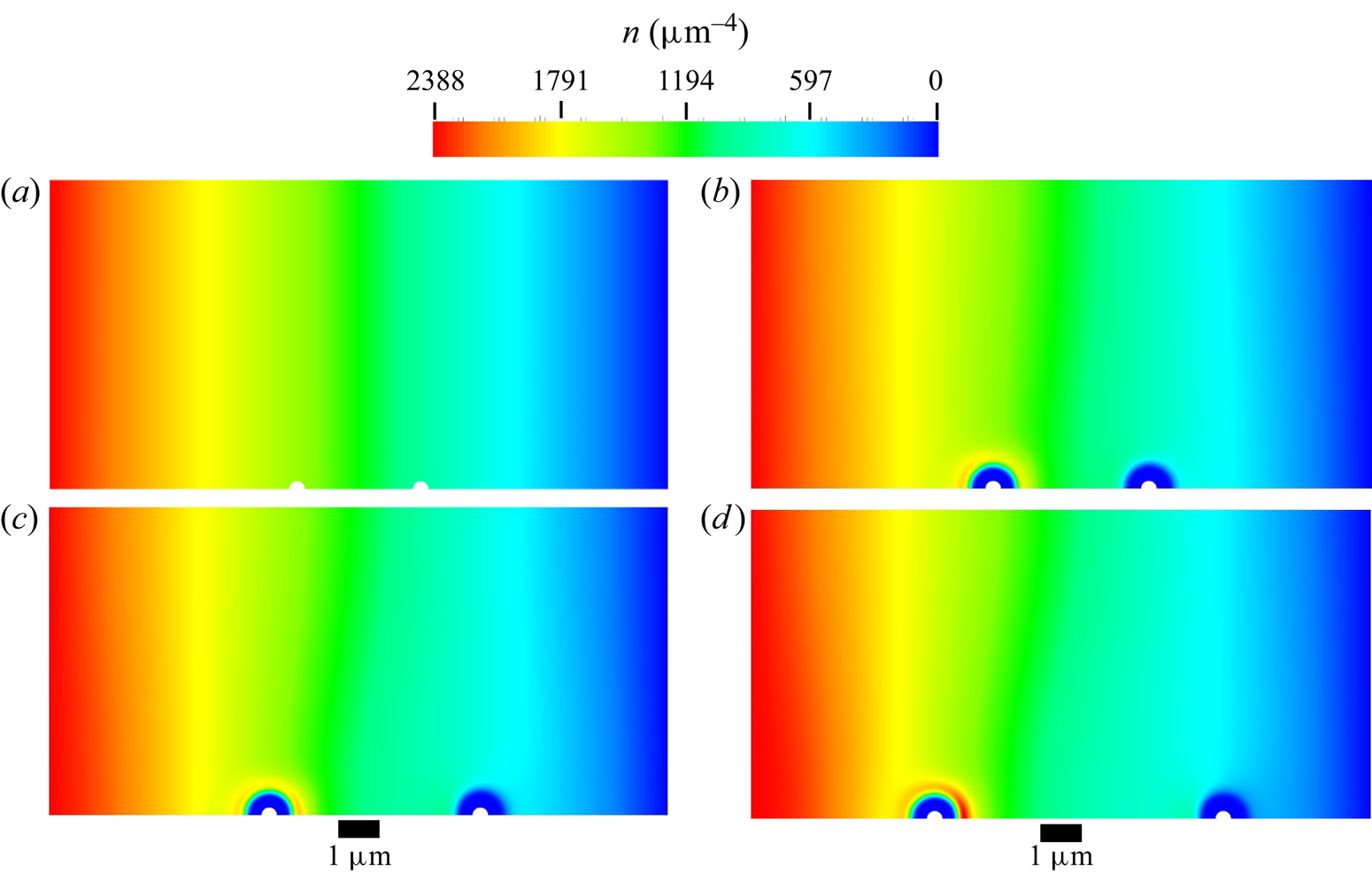
Figure 8. Evolution of solute concentration profile and particle position, illustrating particle separation via diffusiophoresis. Results are shown for (a)  $t = 0$ s, (b)
  $t = 0.003$ s, (c)
  $t = 0.005$ s, (d)
  $t = 0.008$ s.
6.3. Influence of solute concentration, diffusivity and concentration gradient on diffusiophoretic velocities
6.3.1. Numerical data and equation regression
Note that none of the systems discussed so far are permanently at equilibrium. Indeed, the drag forces and solute–interface forces in figure 5 equilibrate each other only at  $n_m=1194 \, {\mathrm {\mu }{\rm m}^{-3}}$. Furthermore, the velocities of the diffusiophoretic particles in figure 7 never reach a plateau: they increase at a low rate even by the end of the simulation. This happens because the equilibrium velocity (i.e. the velocity for which drag and solute–interface forces equilibrate each other) generally depends on the far-field solute concentration
  $n_m$.
There are a few limit cases for which the equilibrium velocity does not depend on  $n_m$. This is true for the HDL (see (2.13)), for steric repulsion when the interaction range is much smaller than the particle radius (Khair Reference Khair2013), and for adsorptive interactions when the range of solute–particle interactions and the adsorption length are much smaller than the particle radius (Anderson & Prieve Reference Anderson and Prieve1984, Reference Anderson and Prieve1991). However, other systems have been described for which equilibrium diffusiophoresis velocity depends on the position of the particle with respect to the far-field solute concentration. For example, the equilibrium velocity
  $v_{DP}$ of a charged particle in an electrolyte solution is proportional to
  ${\boldsymbol {\nabla } n}^\infty / n_m$ (Anderson Reference Anderson1989). This velocity depends not only on the imposed far-field electrolyte concentration gradient
  ${\boldsymbol {\nabla } n}^\infty$, but also on the position of the particle with respect to this far field (
 $n_m$). Indeed, we expect
  $v_{DP}$ to change as the particle moves through the solution, since
  $n_m$ does not remain constant.
The diffusiophoresis velocity also depends on the position of the particle if the adsorption length K is not negligible compared with the particle radius. Anderson & Prieve (Reference Anderson and Prieve1984, Reference Anderson and Prieve1991) derived (2.7) for the diffusiophoresis velocity in this case, assuming that the range of solute–particle interaction (not to be confused with the adsorption length) is much smaller than the particle radius.
Simulation results in table 3 show that the TFCV model presented in § 4.2 also accounts for the velocity dependency on the position featured by  $n_m$. All these simulations were performed according to the solute–interface interaction potential in (4.4).
Table 3. Equilibrium velocities obtained with TFCV for different sets of parameters.
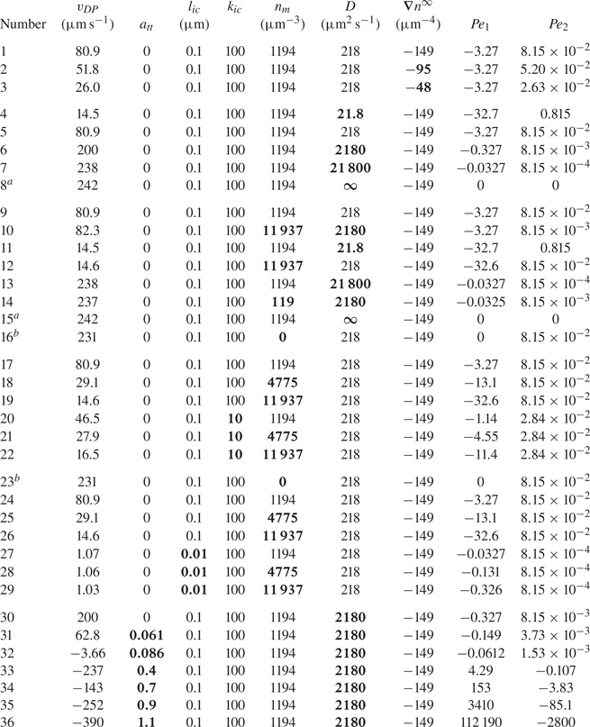
 $^{a}$HDL instead of TFCV.
 $^{b}$Result is purely mathematical and has no physical significance, since
  $n_m=0$ and
  ${\boldsymbol {\nabla } n}^\infty \neq 0$ imply negative solute concentrations in the simulation domain.
 $^{c}$Some data are repeated in the table: (1,5,9,17,24); (4,11); (7,13); (8;15); (16,23); (12,19,26); (18,25).
The first row in this table gives the equilibrium velocity for a reference set of parameters ( $a_{tt}=0$,
  $l_{ic}=0.1\,{\mathrm {\mu }{\rm m}}$,
  $k_{ic}=100$,
  $n_m=1194\,{\mathrm {\mu }{\rm m}^{-3}}$,
  $D=218\,{\mathrm {\mu }{\rm m}^2\,{\rm s}^{-1}}$ and
  ${\boldsymbol {\nabla } n}^\infty =-149\,{\mathrm {\mu }{\rm m}^{-4}}$). Simulations 9–29 prove that the velocity is a function of
  $n_m$. Furthermore, results for
  $l_{ic}=0.01\,{\mathrm {\mu }{\rm m}}$ or
  $k_{ic}=10$ (see (4.4)) show how this dependency is affected by the solute–interface interaction potential. As the interaction width
  $l_{ic}$ decreases from 0.1 to
  $0.01\,{\mathrm {\mu }{\rm m}}$ (simulations 23–29 in table 3), the relative change in velocity with respect to
  $n_m$ is less significant. This is in agreement with previous results obtained for short-range steric repulsions (Khair Reference Khair2013). In addition, velocity variation with respect to
  $n_m$ decreases when the potential magnitude
  $k_{ic}$ decreases from 100 to 10 (simulations 17–22).
Another important feature, shown by simulations 4–7, is that as  $D\to \infty$ the equilibrium velocity approaches the value of
  $242\,{\mathrm {\mu }{\rm m}\,{\rm s}^{-1}}$ obtained assuming HDL (simulation 8). Furthermore, simulations 1–3 show that the velocity is a linear function of
  ${\boldsymbol {\nabla } n}^\infty$. This result is in agreement with the various studies on diffusiophoresis cited in this chapter (Anderson & Prieve Reference Anderson and Prieve1984, Reference Anderson and Prieve1991; Churaev et al. Reference Churaev, Derjaguin and Muller1987; Anderson Reference Anderson1989; Marbach et al. Reference Marbach, Yoshida and Bocquet2020; Ramírez-Hinestrosa et al. Reference Ramírez-Hinestrosa, Yoshida, Bocquet and Frenkel2020). Finally, simulations 9–16 suggest that the velocity depends on the factor
  $D/n_m$, as predicted by Anderson & Prieve (Reference Anderson and Prieve1984, Reference Anderson and Prieve1991) in the limit of a small solute–particle interaction range (2.7).
With these observations, a suitable fitting function could be derived, which approximates the diffusiophoretic velocity in the range of values  $n_m$, D and
  ${\boldsymbol {\nabla } n}^\infty$ shown in table 3. This function is given by
 \begin{equation} v_{DP}={-}C_1 {\boldsymbol{\nabla} n}^\infty \exp{\left(-\frac{C_2}{D/n_m+C_3}\right)}. \end{equation}
 The numerical values regressed for  $C_1$,
  $C_2$ and
  $C_3$ are respectively 1.61393, 0.29199 and 0.08591, all with units of
  ${\mathrm {\mu }{\rm m}^5\,{\rm s}^{-1}}$. Note that this regression was made considering only the simulations with
  $k_{ic}=100$,
  $l_{ic}=0.1\,{\mathrm {\mu }{\rm m}}$ and
  $a_{tt}=0$. In general,
  $C_1$,
  $C_2$ and
  $C_3$ depend on these parameters, as well as on R (SI units: m),
  $\eta$ (SI units:
  ${{\rm kg}\,{\rm m}^{-1}\,{\rm s}^{-1}}$) and
  $k_B T$ (SI units:
  ${{\rm m}^2\,{\rm kg}\,{\rm s}^{-2}}$). Extrapolating (6.3) to any set of problem parameters would be equivalent to assuming that no additional term is hindered in (6.3). For example, the real expression for
  $v_{DP}$ could be the right-hand side of (6.3) plus a term proportional to, say, the square of
  ${\boldsymbol {\nabla } n}^\infty$. However, for the range of parameters shown in table 3, this second term might go to 0, so it does not appear in the regressed equation (6.3).
The pre-exponential term  $C_1$ can be replaced by a general expression for any interface–solute interaction potential. To find this expression, one should consider that (6.3) must also hold in the limit
  $D\to \infty$. Under this limit,
  $v_{DP}$ is given by (2.13). In addition, dimensional analysis can shed light on the expression for the remaining coefficients
  $C_2$ and
  $C_3$. As previously mentioned, these coefficients have SI units of
  ${{\rm m}^5\,{\rm s}^{-1}}$. Other than D, the only parameters in (4.7)–(4.10) that contain a time unit are
  $\eta$ and
  $k_B T$. However, they also happen to be the only parameters containing a mass unit. Therefore,
  $C_2$ and
  $C_3$ are certainly proportional to the ratio
  $k_B T/\eta$ (SI units:
  ${{\rm m}^3\,{\rm s}^{-1}}$). It is tempting to multiply this factor by
  $R^2$ to get the correct units. However, the missing square length unit could also come from a functional of the potential
  $\varPi _{ic}$, such as
  $\int \varPi _{ic} r\,\mathrm {d}r$. Finally,
  $k_B T$ and
  $\eta$ cannot appear in the form of a dimensionless term in the expression of
  $C_2$ and
  $C_3$, since no dimensionless terms can be generated with
  $k_B T$ (SI units:
  ${{\rm m}^2\,{\rm kg}\,{\rm s}^{-2}}$),
  $\eta$ (SI units:
  ${{\rm kg}\,{\rm m}^{-1}\,{\rm s}^{-1}}$) and R (SI units: m). Therefore, the most general expression that can be derived for
  $v_{DP}$ is
 \begin{align}
v_{DP}= \frac{R^2}{3\eta}{\boldsymbol{\nabla} n}^\infty k_B
T \left(\int_R^\infty f(r)(-\varPi_{ic}^\prime)
\left(\frac{r}{R}-\frac{R}{3r}-\frac{2r^2}{3R^2} \right) \,
\mathrm{d}r \right)
\exp{\left(-\frac{C_2^\prime}{\dfrac{D\eta}{k_B T
n_m}+C_3^\prime}\right)},
\end{align}
\begin{align}
v_{DP}= \frac{R^2}{3\eta}{\boldsymbol{\nabla} n}^\infty k_B
T \left(\int_R^\infty f(r)(-\varPi_{ic}^\prime)
\left(\frac{r}{R}-\frac{R}{3r}-\frac{2r^2}{3R^2} \right) \,
\mathrm{d}r \right)
\exp{\left(-\frac{C_2^\prime}{\dfrac{D\eta}{k_B T
n_m}+C_3^\prime}\right)},
\end{align}
where the coefficients  $C_2^\prime$ and
  $C_3^\prime$ (units:
  ${\mathrm {\mu }{\rm m}^2}$) depend on R and
  $\varPi _{ic}$. Regression of these parameters using the data in table 3 gives
  $C_2^\prime =0.070157$ and
  $C_3^\prime =0.020669$, and the comparison between simulated and regressed velocities is shown in figure 9.
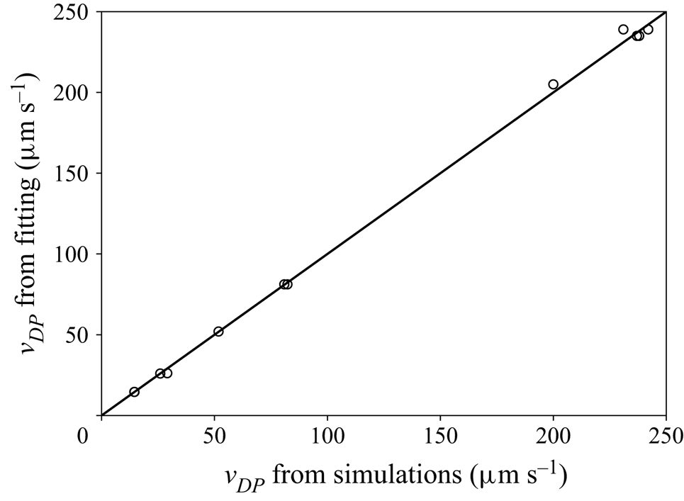
Figure 9. Comparison between diffusiophoretic velocities obtained via simulation ( $x$ axis) and via the fitting equation (6.4) (
 $y$ axis) for
  $k_{ic}=100$,
  $l_{ic}=0.1\,{\mathrm {\mu }{\rm m}}$ and
  $a_{tt}=0$.
Equation (6.4) suggests that the ratio inside the exponential could be a suitable definition for a Péclet number, as follows:
 \begin{equation} {Pe}= \frac{\dfrac{n_m C_2^\prime k_B T}{D \eta}}{1+\dfrac{n_m C_3^\prime k_B T}{D \eta}}. \end{equation}
Such a number could be used as a criterion for the applicability of the ‘infinite diffusivity’ hypothesis in HDL. Indeed, when  ${Pe} \ll 1$, the phoretic velocity no longer depends on diffusivity, and (6.4) becomes (2.13). The problem with such a definition is that the functionals
  $C_2^\prime$ and
  $C_3^\prime$ are unknown. The values regressed for them are only valid for the potential
  $\varPi _{ic}$ given in (4.4), with
  $a_{tt}=0$,
  $l_{ic}=0.1 \, {\mathrm {\mu }{\rm m}}$, and
  $k_{ic}=100$.
Note that the equation regressed for  $v_{DP}$ is only applicable in the case of an externally imposed (constant) far-field gradient. Other situations would have to be treated case by case. For example, in self-diffusiophoresis it is common to set a fix solute concentration far from the sphere,
  $n|_{r\to \infty }=n_\infty =\mathrm {cte}$ (Michelin & Lauga Reference Michelin and Lauga2014). In this case, the parameter
  $n_\infty$ would replace
  ${\boldsymbol {\nabla } n}^\infty$ and
  $n_m$ in table 3, and a completely different equation for
  $v_{DP}$ might have been regressed.
To confirm the validity of (6.4), a random set of values within the ranges shown in table 1 were assigned for  ${\boldsymbol {\nabla } n}^\infty$ (
 $-120\,{\mathrm {\mu }{\rm m}^{-4}}$),
  $n_m$ (
 $1289\,{\mathrm {\mu }{\rm m}^{-3}}$) and D (
 $186\,{\mathrm {\mu }{\rm m}^2\,{\rm s}^{-1}}$). Furthermore, different values were set for
  $\eta$ (
 $2\times 10^{-3}\,{\rm Pa}\,{\rm s}$) and T (273 K). The velocity calculated according to (6.4) is then
  $42.7\,{\mathrm {\mu }{\rm m}\,{\rm s}^{-1}}$, corresponding to a relative error of only -3.6 % when compared with the velocity obtained from simulations (
 $44.3\, {\mathrm {\mu }{\rm m}\,{\rm s}^{-1}}$). Hence, this equation successfully concludes one of the objectives listed in § 3: to derive an expression for the diffusiophoretic velocity as a function of the problem parameters. Despite not describing the dependency on the solute–interface interaction potential in fully explicit terms, it gives a great insight into how the other physical quantities affect diffusiophoresis. In addition, this equation is derived without assuming infinite diffusivity, a thin interaction layer or weak interaction strength. To the best of the author's knowledge, no explicit relation for diffusiophoretic velocities has been derived before without at least one of these assumptions.
6.3.2. Comparison with previous studies
As mentioned in the previous paragraph, the equations for phoretic velocity derived in the literature always make some kind of simplifying assumption. If (6.4) is correct, it should be compatible with these previous equations under some limiting conditions. This section is consecrated to verifying this compatibility.
Equation (2.1) is the first to be derived in the literature. It considers an infinitely thin interfacial layer, neglects solute transport via convection and assumes  $K/R=0$, with K being the adsorption layer defined in (2.2a) and R being the sphere radius. Such an equation is indeed compatible with (2.1). To see this, let us first assess the effect of neglecting solute transport via convection. This amounts to setting the diffusion coefficient D to infinity, yielding (2.13). This equation can be further simplified with the infinitely thin diffusive/adsorption layer assumptions. To obtain this, one needs to change the variable
  $r$ to
  $y=r-R$ in the integral, and then use the hypothesis to set the ratio
  $y/R$ tending to 0,
 \begin{align} \left. \begin{aligned} v_{DP} & = \frac{R^2}{3\eta}{\boldsymbol{\nabla} n}^\infty k_B T \int_0^\infty f(R+y)(-\varPi_{ic}^\prime) \left(\frac{y+R}{R}-\frac{R}{3(y+R)}-\frac{2(y+R)^2}{3R^2} \right) \, \mathrm{d} y \implies \\ v_{DP} & = \frac{R^2}{3\eta}{\boldsymbol{\nabla} n}^\infty k_B T \int_0^\infty f(R+y)(-\varPi_{ic}^\prime) \left(\frac{y}{R}+1-\frac{1}{3}\left(\frac{y}{R}+1\right)^{{-}1}\right.\\ & \qquad \left.-\frac{2}{3}\left(\frac{y}{R}\right)^2-\frac{4}{3}\frac{y}{R}-\frac{2}{3} \right) \, \mathrm{d} y \implies \\ v_{DP} & = \frac{R^2}{3\eta}{\boldsymbol{\nabla} n}^\infty k_B T \int_0^\infty f(R+y)(\varPi_{ic}^\prime) \left( \left(\frac{y}{R} \right)^2 + O\left(\frac{y}{R}\right)^3 \right) \, \mathrm{d} y \implies\\ v_{DP} & = \frac{k_B T}{3\eta}{\boldsymbol{\nabla} n}^\infty \int_0^\infty f(R+y)(\varPi_{ic}^\prime) \left( y^2 +y^2 O\left(\frac{y}{R}\right) \right) \, \mathrm{d} y \implies\\ v_{DP} & = \frac{k_B T}{3\eta}{\boldsymbol{\nabla} n}^\infty \int_0^\infty f(R+y)(\varPi_{ic}^\prime) y^2 \, \mathrm{d} y. \end{aligned} \right\} \end{align}
 Anderson & Prieve (Reference Anderson and Prieve1991) give the solute concentration profile near the sphere for the infinitely thin boundary layer case. Replacing such a profile into (2.10) gives  $f(r)$ inside the interfacial layer,
 \begin{equation} f(r) = \frac{3}{2}\mathrm{e}^{-\varPi_{ic}}. \end{equation}
Inserting (6.7) into (6.6) and using integration by parts yields for an infinitely thin boundary layer,
 \begin{equation} \left. \begin{aligned} v_{DP} & = \frac{k_B T}{2\eta}{\boldsymbol{\nabla} n}^\infty \int_0^\infty \mathrm{e}^{-\varPi_{ic}}(\varPi_{ic}^\prime) y^2 \, \mathrm{d} y \implies \\ v_{DP} & = \frac{k_B T}{2\eta}{\boldsymbol{\nabla} n}^\infty \left[\left. y^2\left(1-\mathrm{e}^{-\varPi_{ic}}\right)\right\rvert_0^\infty- \int_0^\infty \left(1-\mathrm{e}^{-\varPi_{ic}}\right) 2y \, \mathrm{d} y \right]. \end{aligned} \right\} \end{equation}
 The left term inside the square brackets in (6.8) is the difference between the expression  $y^2(1-\mathrm {e}^{-\varPi _{ic}})$ evaluated at
  $y=\infty$ and at
  $y=0$. At
  $y=0$, this expression equals 0. At
  $y=\infty$,
  $\varPi _{ic}$ goes to 0, and the limit is a priori indeterminate. To evaluate it, let us use the Taylor expansion of
  $\mathrm {e}^{-\varPi _{ic}}$,
 \begin{equation} \lim_{y\to\infty}{y^2\left(1-\mathrm{e}^{-\varPi_{ic}}\right)} = \lim_{y\to\infty}{y^2\left(\varPi_{ic} + O\left({\varPi_{ic}}^2\right)\right)}. \end{equation}
 It can be shown from (4.6) that the interaction potential  $\varPi _{ic}$ must be
  $o(1/y^2)$ when
  $y\to \infty$. Otherwise, the solute would apply an infinite force on the solvent. Replacing
  $\varPi _{ic}$ by
  $o(1/y^2)$ in (6.9) yields
 \begin{equation} \lim_{y\to\infty}{y^2\left(1-\mathrm{e}^{-\varPi_{ic}}\right)} = 0. \end{equation}
Finally, inserting (6.10) into (6.8) yields (2.1), proving that (6.4) is in agreement with (2.1) in the limit of infinitely thin interfacial layers.
Anderson & Prieve (Reference Anderson and Prieve1991) also give the solute concentration profile for an arbitrary length K of the adsorption layer, and under the assumptions of an infinitely thin interfacial layer and absence of solute transport via convection. Inserting this expression into (2.10) gives
 \begin{equation} f(r) = \left(1+\frac{1}{2}\frac{1-2K/R}{1+K/R}\right)\mathrm{e}^{-\varPi_{ic}}. \end{equation}
 Inserting (6.11) into (6.6), integrating by parts and neglecting the terms that are  $o(K/R)$ yields (2.3).
When convection takes place, (6.6) for an infinitely thin diffusive layer must be rewritten taking into account the exponential term in (6.4),
 \begin{equation} v_{DP} = \frac{k_B T}{3\eta}{\boldsymbol{\nabla} n}^\infty \exp{\left(-\frac{C_2^\prime}{\dfrac{D\eta}{k_B T n_m}+C_3^\prime}\right)} \int_0^\infty f(R+y)(\varPi_{ic}^\prime) y^2 \, \mathrm{d} y. \end{equation}
 The function  $f(r)$ remains the one defined in (6.11), even though convection is taken into account. This is because such a function is related to the solute concentration profile in the absence of convection, as described in § 4.3. Therefore, one should insert (6.11) into (6.12). Integration by parts then yields
 \begin{equation} v_{DP}= L^*K\dfrac{k_B T}{\eta} {\boldsymbol{\nabla} n}^\infty \left(\dfrac{1}{1+\dfrac{K}{R}}\right) \exp{\left(-\dfrac{C_2^\prime}{\dfrac{D\eta}{k_B T n_m}+C_3^\prime}\right)}. \end{equation}
 In order to retrieve (2.5) or (2.7), (6.13) has to be written in terms of the Péclet number  ${{Pe}_1}$ defined in (2.4a),
 \begin{equation} v_{DP}= L^*K\dfrac{k_B T}{\eta} {\boldsymbol{\nabla} n}^\infty \left(\dfrac{1}{1+\dfrac{K}{R}}\right) \exp{\left(-\dfrac{\dfrac{C_2^\prime}{L^*K}}{\dfrac{1}{{{Pe}_1}}+\dfrac{C_3^\prime}{L^*K}}\right)}. \end{equation}
 Note that the Péclet number  ${{Pe}_1}$ given by (2.4a) can be arbitrarily small or large depending on the diffusion coefficient (cf. table 3). Therefore, to justify a Taylor expansion of the exponential term in (6.14), one must have
 \begin{equation} \frac{\dfrac{C_2^\prime}{L^*K}}{\dfrac{1}{{{Pe}_1}}+\dfrac{C_3^\prime}{L^*K}} \ll 1. \end{equation}
 We recall that  $C_2^\prime$ and
  $C_3^\prime$ are functionals of the interaction potential
  $\varPi _{ic}$, and we shall assume that (6.15) holds in the limit of infinitely thin interfacial layers. Using the first-order approximation of the exponential term in (6.14) yields
 \begin{equation} v_{DP}= L^*K\dfrac{k_B T}{\eta} {\boldsymbol{\nabla} n}^\infty \left(\dfrac{1}{1+\dfrac{K}{R}}\right) \left[ 1-\left(\dfrac{\dfrac{C_2^\prime}{L^*K}}{\dfrac{1}{{{Pe}_1}}+\dfrac{C_3^\prime}{L^*K}}\right)\right]. \end{equation}
Finally, comparison between (6.16) and (2.7) gives the sufficient conditions for compatibility between (6.4) and (2.7). In the limit of infinitely thin interfacial layers, one must have
 \begin{equation} C_2^\prime, C_3^\prime \to \frac{\nu L^* K^2}{K+R}, \end{equation}
where  $\nu$ is given by (2.6).
Because (2.5) is the first-order approximation of (2.7) when  ${{Pe}_1} \ll 1$, it follows that (2.5) is also a special case of (6.4). Equation (2.5) gives good predictions for
  $v_{DP}$ in simulations 27–29, with relative errors between 3.7 % and 4.1 %. This good agreement comes from the fact that these simulations considered a small solute–interface interaction range (
 $l_{ic}=0.01\,{\mathrm {\mu }\textrm {m}}$), and hence, the hypothesis of a thin interfacial layer holds. And with that, we conclude that the equation regressed in § 6.3.1 is in agreement with (2.1), (2.3), (2.5) and (2.7), the latter four being special cases of the former under some limiting conditions.
In § 2 an additional equation for the phoretic velocity is given (2.8), derived by Keh & Weng (Reference Keh and Weng2001). This equation agrees with (2.7), and consequently with (6.4), when  ${{Pe}_2} \to 0$. However, for finite values of
  ${{Pe}_2}$ (defined in (2.4b)), the expression in (2.8) is different from (6.4). Indeed, the latter stipulates a linear relationship between
  ${\boldsymbol {\nabla } n}^\infty$ and
  $v_{DP}$, whereas in the former such a relation is nonlinear due to the terms depending on
  ${{Pe}_2}$. This discrepancy could be due to the fact that the term on
  ${{Pe}_2}^2$ in (2.8) is always much smaller than 1 for the data set shown in table 3. Indeed, even though
  ${{Pe}_2}$ can be as high as 0.8, the maximum value of the product
  $\alpha _2 {{Pe}_2}^2$ in table 3 is 0.0058 (for simulation 4/11). This might be why the data does not capture the nonlinearity with respect to the solute concentration gradient.
Furthermore, some of the steps in the derivation of (2.8) by Keh & Weng (Reference Keh and Weng2001) are unclear. For example, it seems that the authors neglect the effect of solute–interface interactions inside the interfacial layer when writing the solute transport equation (17). Moreover, they use the quasi-steady hypothesis to replace the transient term  $\partial n / \partial t$ in the solute mass balance equation (3) by
  ${\boldsymbol {\nabla } n}^\infty v_{DP}$ in equation (17). These premises are not necessarily true, and might result in incorrect inferences in some cases. For example, let us assess the case of interactions due exclusively to steric exclusion. The interface–solute interaction potential in this case can be written as
 \begin{equation} \varPi_{ic} = \left\{ \begin{array}{ll} +\infty, & y\le a, \\ 0, & y>a, \end{array} \right. \end{equation}
where a is the size of the solute particles and y is the distance between the interface and a point in the mixture domain.
In this case,  $K=-a$ and
  $L=a/2$. If solute advection is neglected, the solute concentration profile inside the diffusive layer, according to equation (43) in Keh & Weng (Reference Keh and Weng2001), is
 \begin{equation} n=n_m+\left(\dfrac{r}{R}+ \dfrac{1+\dfrac{2a}{R}}{2\left(1-\dfrac{a}{R}\right)} \dfrac{R^2}{r^2}\right){\boldsymbol{\nabla} n}^\infty \cos(\theta). \end{equation}
 This means that for every point inside the diffusive layer on  $\theta ={\rm \pi} /2$ or
  $\theta =3{\rm \pi} /2$, the concentration equals
  $n_m$. This is obviously false, since steric exclusion implies 0 solute concentration around the interface. Furthermore, the solute flux across the sphere is not equal to 0 for the solute concentration profile given in (6.19). It might be that the work by Keh & Weng (Reference Keh and Weng2001) is only applicable in the context of adsorption, even though such a restriction is not explicitly mentioned by the authors.
6.4. Influence of solute–interface interactions on diffusiophoretic velocity
The last set of simulations in table 3 (30–36) shows the variation of  $v_{DP}$ with respect to the attraction parameter
  $a_{tt}$ modulating the solute–interface interactions. For purely repulsive interactions, the sphere moves against the solute concentration gradient. However, as
  $a_{tt}$ increases this tendency is inverted. Note that the effect of this parameter on the diffusiophoretic velocity is non-monotonic:
  $v_{DP}$ decreases from
  $a_{tt}=0$ to
  $a_{tt}=0.4$, increases from
  $a_{tt}=0.4$ to
  $a_{tt}=0.7$, and decreases again for
  $a_{tt}>0.7$. A similar behaviour is mentioned in § 1, when the paper by Ramírez-Hinestrosa et al. (Reference Ramírez-Hinestrosa, Yoshida, Bocquet and Frenkel2020) is discussed. Figure 10 compares the variations in particle mobility as a function of
  $a_{tt}$ (present study) and as a function of the solute–monomer dispersion energy
  $\epsilon _{ms}$ (Ramírez-Hinestrosa et al. Reference Ramírez-Hinestrosa, Yoshida, Bocquet and Frenkel2020).

Figure 10. (a) Particle mobility versus attraction parameter, according to fluid simulation results in table 3; (b) particle mobility versus solute–monomer dispersion energy  $\epsilon _{ms}$, according to molecular simulations (extracted from Ramírez-Hinestrosa et al. (Reference Ramírez-Hinestrosa, Yoshida, Bocquet and Frenkel2020) with permission from AIP publishing).
The definition of mobility changes slightly between both works: whereas the present paper defines mobility as  $\varGamma =v_{DP}/{\boldsymbol {\nabla } n}^\infty$, Ramírez-Hinestrosa et al. (Reference Ramírez-Hinestrosa, Yoshida, Bocquet and Frenkel2020) set
  $\varGamma =v_{DP}/F_{s}$, where
  $F_{s}$ is an external force acting on the solute particles. However, this difference does not prevent a comparison between results, as the external force considered in the molecular simulations mimics the effect of explicit concentration gradients.
Both plots in figure 10 show an initial increase in mobility as the solute–interface attraction becomes stronger. When repulsion dominates over attraction (small  $a_{tt}$ and
  $\epsilon _{ms}$ values), the particle moves towards lower solute concentrations, and
  $\varGamma <0$. Zero mobility is attained for
  $a_{tt}=0.086$ (figure 10a) and for
  $\epsilon _{ms}=1\epsilon _0$ (figure 10b), where
  $\epsilon _0$ is a reference energy. The latter result is almost trivial after a closer look into the paper by Ramírez-Hinestrosa et al. (Reference Ramírez-Hinestrosa, Yoshida, Bocquet and Frenkel2020). In that paper, the authors simulate solute–solute, solute–solvent, solvent–solvent, solvent–monomer and solute–monomer interactions via a 12-6 Lennard–Jones potential, setting all the binary interaction lengths to
  $\sigma _0$. Furthermore, all dispersion energies are set to
  $1\epsilon _0$, except possibly for solute–monomer interactions
  $\epsilon _{ms}$. When
  $\epsilon _{ms}=1\epsilon _0$, the monomers are indistinguishable from solute and solvent molecules, and diffusiophoresis no longer takes place. The same is not true for the macroscopic approach that generated figure 10(a). Indeed, even when
  $v_{DP}$, and thus mobility, approaches 0 (simulation 32 in table 3), the effect of the interface on the mixture was very pronounced. It changes solute distribution significantly near the sphere and drives diffusioosmotic flow (profiles not shown for brevity).
When attraction dominates over repulsion, the interface tends to move towards higher solute concentrations, and  $\varGamma >0$. Particle mobility continues to increase with respect to
  $a_{tt}$ and
  $\epsilon _{ms}$ until it reaches a maximum value at
  $a_{tt}=0.4$ and
  $\epsilon _{ms}\approx 2.5\epsilon _0$. A possible reason for this local maximum is given by Ramírez-Hinestrosa et al. (Reference Ramírez-Hinestrosa, Yoshida, Bocquet and Frenkel2020): as the adsorption interactions get stronger, the solute particles surrounding the sphere become immobilized, hindering diffusiophoresis. Reasoning in mathematical terms for the case study in figure 1, the solute distribution around the interface becomes more symmetric as the attraction parameter increases, decreasing the resultant force exerted by the solute on the sphere.
The systems start to behave differently for large attraction parameters: whereas Ramírez-Hinestrosa et al. (Reference Ramírez-Hinestrosa, Yoshida, Bocquet and Frenkel2020) predict an asymptotic decay for the mobility, this work has found that the mobility reaches a minimum (for  $a_{tt}=0.7$) and then increases indefinitely. Some possible explanations for this discrepancy are listed below.
(i) Ramírez-Hinestrosa et al. (Reference Ramírez-Hinestrosa, Yoshida, Bocquet and Frenkel2020) considered a truncated potential, whereas in this work the interface can interact with the solute everywhere in the domain. To understand how this may affect the behaviour of the curves in figure 10, let us briefly summarize the discussion from the previous paragraphs. As the adsorption strength increases, the strength of solute–interface attraction increases, and the interface tends to move faster and faster towards higher solute concentrations. However, after a certain threshold, the increase in the individual interaction forces is offset by the increasing symmetry of the solute concentration profile, and mobility starts decreasing. In other words, even though the attraction between individual solute molecules and the interface is stronger, these forces cancel each other due to the radial symmetry of the solute concentration profile around the sphere. This explains the local maximum at
 $a_{tt}=0.4$ and $\epsilon _{ms}\approx 2.5\epsilon _0$. In the paper by Ramírez-Hinestrosa et al. (Reference Ramírez-Hinestrosa, Yoshida, Bocquet and Frenkel2020), the monomer–solute interaction potential is truncated at a certain distance $\sigma$. If $\epsilon _{ms}$ is large enough, the entire range of interaction $\sigma$ may be immobilized, and $\varGamma$ will decrease asymptotically according to figure 10(b). On the other hand, $\varPi _{ic}$ used in this work is not truncated, and an increase in $a_{tt}$ will also increase the range of interaction between the sphere and the solute. For $a_{tt}>0.7$, this effect probably overcomes the increasing symmetry of the solute distribution, and the mobility starts increasing again with respect to $a_{tt}$.
(ii) In the fluid simulation models we have described in § 4, solute–solute interactions are neglected. However, the size of the solute particles in the mixture is accounted for in molecular simulations via the solute–solute Lennard–Jones potential, which limits solute accumulation around the polymer. These solute–solute interactions surely play an important role in Ramírez-Hinestrosa et al. (Reference Ramírez-Hinestrosa, Yoshida, Bocquet and Frenkel2020), since solute molar fraction in the bulk was set to 0.5 in their work. Other simplifying assumptions in the models described here, such as incompressible fluid and constant viscosity (i.e. viscosity independent of solute concentration) may also contribute to the discrepancies seen in figure 10.
(iii) The small size of the polymer in the molecular simulations by Ramírez-Hinestrosa et al. (Reference Ramírez-Hinestrosa, Yoshida, Bocquet and Frenkel2020) makes the problem fundamentally different from the case study investigated here (figure 1). For small ratios between the molecular mean free path and characteristic length of the system, molecular simulations are generally in agreement with the governing (continuum) equations for fluid dynamics and solute transport (Zhang & Ma Reference Zhang and Ma2020). However, in the work by Ramírez-Hinestrosa et al. (Reference Ramírez-Hinestrosa, Yoshida, Bocquet and Frenkel2020) the representative physical length scale for the phenomenon is the size of the polymer, which is close to the mean free path of the solvent molecules. Indeed, figure 10(b) considers a polymer made of 30 monomers; when
$\epsilon _{ms}=8\epsilon _0$, the equivalent hydrodynamic radius of the polymer is $R_p\approx 2.4\sigma _0$, comparable to the mean free path $l_{free}\approx \sigma _0$ of solvent molecules (the length parameter in the Lennard–Jones potential). It is recalled that the representative physical length scale in the case study shown in figure 1 is $R=0.2\, {\mathrm {\mu }\textrm {m}}$, which is several orders of magnitude higher than the molecular spacing in liquid water. It is possible that this difference in the orders of magnitude makes the works incomparable. Still, it is interesting to note that, as $\epsilon _{ms}$ decreases, the hydraulic radius of the polymer increases (e.g. $R_p\approx 4.8\sigma _0$ when $\epsilon _{ms}=1.5\epsilon _0$). And it is precisely in the region of low $\epsilon _{ms}$ (and low $a_{tt}$) that qualitative agreement exists between the curves in figure 10. This could be because the higher hydraulic radius at low $\epsilon _{ms}$ makes the polymer diffusiophoresis phenomenon more ‘continuum like’.


7. Conclusion
This paper has covered various aspects of diffusiophoresis through numerical simulations. Three different models were used to achieve different goals. The TEF was used to assess the actual dynamics of a diffusiophoretic system. The numerical simulations using this model allow us for instance to capture the effect of overlapping diffusive layers in particle separation. From these simulations it was found that diffusiophoresis may be suitable for particle separation, as shown in § 6.2. Overall, this section stresses the robustness of the simulation set-up used in this paper, indicating that it could be used to quickly screen parameters and configurations that allow better/worst particle separation.
The second model discussed in this paper, called TFCV, was used in combination with TEF to demonstrate that diffusiophoretic systems ‘forget’ their initial state after a certain amount of time (see figures 5–7). Transient formulation at constant velocity alone was employed to regress the mathematical expression (6.4) that relates the diffusiophoretic velocity to  $n_m$, D,
  ${\boldsymbol {\nabla } n}^\infty$,
  $k_B T$ and
  $\eta$. In the limit of infinite diffusivity, this expression converges to (2.13) derived by Marbach et al. (Reference Marbach, Yoshida and Bocquet2020). Furthermore, it agrees with the previous works placed in the limit of infinitesimally thin solute–interface interaction layers (Derjaguin et al. Reference Derjaguin, Sidorenkov, Zubashchenkov and Kiseleva1947; Anderson & Prieve Reference Anderson and Prieve1984, Reference Anderson and Prieve1991).
Transient formulation at constant velocity was also used to investigate the effect of long-range solute–interface attraction on the particle mobility. This study was performed by varying the parameter  $a_{tt}$ in (4.4). It was found that the mobility changes with respect to
  $a_{tt}$ in a non-monotonic way, as illustrated in figure 10(a). The results were compared with those from a benchmark work on molecular simulations applied to diffusiophoresis (Ramírez-Hinestrosa et al. Reference Ramírez-Hinestrosa, Yoshida, Bocquet and Frenkel2020). Both studies agree in the range of small attraction forces, showing an inversion of particle mobility after a certain attraction threshold, followed by a peak of maximum phoretic mobility and a subsequent decrease (figure 10). However, discrepancies arise as attraction forces are further increased. Ramírez-Hinestrosa et al. (Reference Ramírez-Hinestrosa, Yoshida, Bocquet and Frenkel2020) predict that mobility decreases asymptotically in the limit of strong attraction interactions, whereas the present study predicts that mobility reaches a local minimum and then increases indefinitely as
  $a_{tt}\to \infty$. Probable reasons for this discrepancy are listed at the end of § 6.4.
Finally, the HDL was used first to validate the mesh used for simulations. This was done by setting  $\varPi _{ic}$ according to (5.1). Such a suitable choice results in the fully analytic expression (5.3) for diffusiophoretic velocity, which can be compared with
  $v_{DP}$ obtained via numerical simulations. In addition, HDL can be used to verify whether the TFCV implementation behaves properly at high D values, according to simulations 4–8 in table 3.
Supplementary material
Supplementary material containing the C routines for user-defined functions used in the simulations is available at https://doi.org/10.1017/jfm.2022.1067.
Funding
This research received no specific grant from any funding agency, commercial or not-for-profit sectors.
Declaration of interests
The authors report no conflict of interest.


 Open access