


1. Introduction
The interaction between shock waves and turbulent boundary layers represents a major challenge for modern aerospace research, given its occurrence in a broad range of engineering applications involving transonic, supersonic and hypersonic systems. Typical examples include high-speed intakes, over-expanded rocket nozzles, transonic airfoil buffeting and the aerodynamics of high-speed vehicles or space launchers. shock wave/turbulent boundary-layer interactions (STBLIs) must carefully be taken into account in the design process, since they can harmfully impact the performance of aerospace systems by enhancing aerodynamic drag and heat transfer at the wall. The adverse pressure gradient imposed by the shock can dramatically alter the structure of the boundary layer, inducing its thickening and, in the case of strong interactions, large-scale separation. The latter is usually associated with concurrent complex phenomena such as amplification of turbulence and noise, formation of large-scale vortical structures and unsteadiness involving a wide range of spatial and temporal scales. Due to their relevance from the technological and scientific standpoint, STBLIs have been an active research field for more than five decades, as demonstrated by the numerous review articles about the topic (Green Reference Green1970; Adamson & Messiter Reference Adamson and Messiter1980; Delery Reference Delery1985; Dolling Reference Dolling2001; Gaitonde Reference Gaitonde2015).
One of the most gripping aspects of STBLI is the low-frequency unsteadiness of the system, which consists of the appearance of streamwise oscillations of a separation shock characterised by a broadband motion at frequencies well below the typical time scales associated with fine-grained turbulence in the upstream boundary layer. It has been highlighted that the shock motion exhibits unsteady features that are similar among various STBLIs in different two- and three-dimensional canonical geometries, such as compression ramps, reflected shocks and blunt and sharp fins. Several experimental and numerical works have greatly contributed to shed some light on the origin of this unsteadiness, for which different mechanisms have been proposed (Erengil & Dolling Reference Erengil and Dolling1991; Beresh, Clemens & Dolling Reference Beresh, Clemens and Dolling2002; Humble et al. Reference Humble, Elsinga, Scarano and van Oudheusden2009), mainly divided into two categories. On the one hand, according to the upstream mechanisms, the source of the unsteadiness is the presence of low-frequency flow structures in the incoming turbulent boundary layer (Andreopoulos & Muck Reference Andreopoulos and Muck1987; Ganapathisubramani, Clemens & Dolling Reference Ganapathisubramani, Clemens and Dolling2009); on the other hand, according to the downstream mechanisms, the unsteadiness is related to the breathing motion of the separation bubble behind the shock, which expands and contracts periodically (Piponniau et al. Reference Piponniau, Dussauge, Debiève and Dupont2009; Touber & Sandham Reference Touber and Sandham2009). Although a general consensus has still not been reached, it has been argued that both mechanisms always coexist in all STBLIs: the downstream mechanism dominates for strongly separated flows, whereas a combined mechanism dominates for weakly separated flows (Clemens & Narayanaswamy Reference Clemens and Narayanaswamy2009).
In the last decade, several studies have exploited high-fidelity simulation data sets to extract the relevant dynamical features of both compression ramps and oblique shock reflections (Pirozzoli et al. Reference Pirozzoli, Larsson, Nichols, Bernardini, Morgan and Lele2010; Grilli et al. Reference Grilli, Schmid, Hickel and Adams2012; Nichols et al. Reference Nichols, Larsson, Bernardini and Pirozzoli2017; Martelli et al. Reference Martelli, Saccoccio, Ciottoli, Tinney, Baars and Bernardini2020; Bakulu et al. Reference Bakulu, Lehnasch, Jaunet, Goncalves da Silva and Girard2021). For example, Priebe et al. (Reference Priebe, Tu, Rowley and Martín2016) applied dynamic mode decomposition (DMD) to the data obtained through direct numerical simulation (DNS) of a Mach 2.9 compression ramp STBLI, and found a strong similarity between DMD modes and linear stability modes reported in the literature. Furthermore, they revealed the existence of streamwise elongated regions of low and high momentum extending from the shock foot in the downstream flow that the authors interpreted as reminiscent of Görtler-like vortices, already observed in previous studies (Loginov, Adams & Zheltovodov Reference Loginov, Adams and Zheltovodov2006). Similar findings were reported by Pasquariello, Hickel & Adams (Reference Pasquariello, Hickel and Adams2017), who performed a wall-resolved, long-time integrated large-eddy simulation (LES) of a high Reynolds number STBLI at Mach 3 with massive flow separation. Their sparsity-promoting DMD identified two types of modes: a low-frequency mode involving the main actors of the interaction (shock system, separated shear layer and separation bubble) associated with the classical breathing motion of the recirculating flow, and medium-frequency modes associated with the shear-layer vortices produced at the shock foot and convected downstream.
To better understand the unsteadiness of the STBLI system, time series extracted from the numerical or the experimental fluid domain are usually analysed by means of the classical Fourier transform. This standard technique is typically used to generate frequency spectra of the physical variables, to determine the energy content of the signals at each frequency and has been applied extensively to characterise the motion of the reflected shock in STBLI, as reported in several works (Clemens & Narayanaswamy Reference Clemens and Narayanaswamy2014). However, according to Bell & Lepicovsky (Reference Bell and Lepicovsky1995), such an approach is fundamentally justified only when stationary or periodic ergodic data are measured over a long time. In fact, for highly unsteady and irregular time series, Fourier transform may misrepresent localised features of the signal in a time-averaged sense, which would distort the representation of the actual physical phenomena taking place (Huang et al. Reference Huang, Shen, Long, Wu, Shih, Zheng, Yen, Tung and Liu1998). The wavelet transform (Mallat Reference Mallat1989; Daubechies Reference Daubechies1992) is instead an analysis tool well suited to the study of multi-scale and non-stationary processes. Indeed, decomposing a time series into the time/temporal-scale space makes it possible to detect the localised variations of the energy within the signal, through a localised counterpart of the standard Fourier spectrum. As a result, wavelet transform allows the detection of intermittent or modulated features in complex flows. On the basis of such properties, wavelet analysis has provided valuable insight into fluid mechanics (Liandrat & Moret-Bailly Reference Liandrat and Moret-Bailly1990), as attested by its use for the study of turbulence (Farge Reference Farge1992; Farge et al. Reference Farge, Kevlahan, Perrier and Schneider1999), aeroacoustics (Grizzi & Camussi Reference Grizzi and Camussi2012; Camussi, Di Marco & Castelain Reference Camussi, Di Marco and Castelain2017), transonic buffet (Kouchi et al. Reference Kouchi, Yamaguchi, Koike, Nakajima, Sato, Kanda and Yanase2016) and over-expanded nozzles (Martelli et al. Reference Martelli, Ciottoli, Bernardini, Nasuti and Valorani2017). However, only very few works have used it to characterise the low-frequency unsteadiness in STBLI (Poggie & Smits Reference Poggie and Smits1997; Guo, Wu & Liang Reference Guo, Wu and Liang2020), and none of them performed such an analysis on a detailed DNS database. Moreover, given the fact that intermittency is defined by the presence of localised bursts of high-energy activity, wavelets can represent a suitable basis also to map and estimate the importance of rare but strong events: a task that could be hardly fulfilled by the trigonometric functions used in the Fourier transform, because of their infinite support in the time domain.
In this work, we present novel DNS data of an oblique shock wave impinging on a turbulent boundary layer inspired by the experiment performed at the IUSTI's hypo-turbulent supersonic wind tunnel and described in Dupont, Haddad & Debiève (Reference Dupont, Haddad and Debiève2006) and Dupont et al. (Reference Dupont, Piponniau, Sidorenko and Debiève2008). The flow we simulated is characterised by a Mach number equal to 2.28 and a momentum-based Reynolds number  $Re_\theta$ equal to 6900. Several groups have previously studied the same flow case either at the same conditions of the experiment, using LES (Touber & Sandham Reference Touber and Sandham2009; Morgan et al. Reference Morgan, Duraisamy, Nguyen, Kawai and Lele2013; Agostini, Larchevêque & Dupont Reference Agostini, Larchevêque and Dupont2015), or using DNS, but at a reduced Reynolds number (Pirozzoli & Bernardini Reference Pirozzoli and Bernardini2011a), because of the hindering computational burden associated with the simulation. Unlike STBLIs at low Reynolds numbers (Dolling & Or Reference Dolling and Or1985; Adams Reference Adams2000; Pasquariello et al. Reference Pasquariello, Grilli, Hickel and Adams2014; Nichols et al. Reference Nichols, Larsson, Bernardini and Pirozzoli2017), in which the viscosity diffuses the separation shock into a milder compression fan, the moderate Reynolds number considered allows the shock foot to penetrate more deeply into the boundary layer. As a result, the inviscid pressure jump of the oscillating shock leaves a direct footprint in the wall pressure, which exhibits a clear and definite intermittency. For lower Reynolds number, instead, since the compression is less sharp, the transition between the pressure states before and after the shock is smoother, which results in an attenuated intermittency and a broader range of frequencies covered by the shock unsteadiness (Ringuette et al. Reference Ringuette, Bookey, Wyckham and Smits2009). Thanks to the possibility of considering the direct trace of the shock unsteadiness at the wall, we are able to perform an exhaustive wavelet analysis on the wall-pressure signal that demonstrates the power of a description of the STBLI unsteadiness in the time/time-scale domain. The continuous wavelet transform is first directly applied to the unsteady signal of the pressure at the wall, to identify the time evolution of the temporal scales characterising the wall-pressure signature of the present STBLI. Then, we use a wavelet-based indicator to evaluate the degree of intermittency of the wall pressure, and to extract from the signal its most energetic, intermittent part. Inspired by Poggie & Smits (Reference Poggie and Smits1997) and by Camussi & Bogey (Reference Camussi and Bogey2021), we propose to use the wavelet transform to filter the wall pressure and to separate the contributions from the flow turbulence and the separation shock unsteadiness. Our work tries thus to exploit the compact support of the wavelet basis to highlight the intermittent nature of the large-scale unsteadiness of the system and to define a practical procedure to extract relevant sparse features from signals of interest for the system modelling. The development of similar procedures to process the pressure – but also other quantities – is a prerequisite for further investigations on STBLI systems.
Finally, we consider the dynamics of the separation bubble behind the separation shock. According to aforementioned theoretical, experimental and numerical works (Dupont et al. Reference Dupont, Haddad and Debiève2006; Piponniau et al. Reference Piponniau, Dussauge, Debiève and Dupont2009; Pasquariello et al. Reference Pasquariello, Hickel and Adams2017), the motion of the shock system – especially for strong interactions – is strictly related to the breathing motion of the separated region. For this reason, we attempt to relate the intermittent features of the wall pressure at the foot of the separation shock to the dynamics of the separation bubble, by replicating the wavelet intermittency analysis on a signal recording an estimate of the recirculation region extent on a single vertical slice throughout the duration of the simulation. Wavelet cross-spectra and wavelet coherence are also considered to estimate the relationship between the wall pressure at the shock foot and the area of the separation bubble.
The paper is organised as follows: § 2 presents the numerical set-up of the simulations; § 3 describes the database generated and the validation carried out; § 4 presents the results of the analysis; finally, § 5 reports some final comments.
2. Numerical set-up
The results presented in this work are obtained from DNSs performed using Supersonic TuRbulEnt Accelerated Navier–Stokes Solver (STREAmS) (Bernardini et al. Reference Bernardini, Modesti, Salvadore and Pirozzoli2021), a high-fidelity solver of the compressible Navier–Stokes equations, targeted to canonical wall-bounded turbulent high-speed flows. The code, freely available online, (https://github.com/matteobernardini/STREAmS.) solves the complete set of Navier–Stokes equations for a perfect, heat conducting gas.
The equations are discretised on a Cartesian mesh and solved by means of the finite difference approach. The convective terms are discretised using a hybrid energy-conservative shock-capturing scheme in locally conservative form (Pirozzoli Reference Pirozzoli2010). In particular, a sixth-order, central, energy-preserving flux formulation is adopted in smooth regions of the flow, which ensures a robust and accurate discretisation of the wide range of spatial and temporal scales typical of turbulence, without relying on numerical (artificial) diffusivity. Shock-capturing capabilities are achieved through the Lax–Friedrichs flux vector splitting, where the characteristic fluxes are reconstructed at the interfaces using a fifth-order, weighted essentially non-oscillatory (WENO) reconstructions (Jiang & Shu Reference Jiang and Shu1996). The hybridisation between the central and the WENO scheme is managed by the implementation of a shock sensor that computes the local smoothness of the solution and identifies discontinuities into the flow. Sixth-order, central finite difference approximations are also applied for the discretisation of the viscous terms. The resulting system of ordinary differential equations is integrated in time by means of a third-order, low-storage, Runge–Kutta scheme. The solver is written in Fortran 90 and presents an MPI parallelisation based on a classical domain decomposition. The current version is able to run on NVIDIA multi-graphics processing unit architectures through the CUDA Fortran paradigm. Additional details on the numerical methods and the scalability performance of STREAmS can be found in Bernardini et al. (Reference Bernardini, Modesti, Salvadore and Pirozzoli2021).
3. Database description and validation
The DNS database is inspired to the oblique shock wave/turbulent boundary-layer interaction reported in Dupont et al. (Reference Dupont, Haddad and Debiève2006, Reference Dupont, Piponniau, Sidorenko and Debiève2008), characterised by a free-stream Mach number  $M_\infty = 2.28$, an incidence angle of the shock generator
  $\phi = 8^\circ$ and a Reynolds number
  $Re_\theta = 5100$. In the simulation, the Reynolds number based on the compressible momentum thickness of the incoming turbulent boundary layer and on the free-stream viscosity is equal to
  $Re_{\theta } \approx 6900$, which corresponds to
  $Re_{\delta _2} \approx 3900$ if wall viscosity is considered. The main properties of the upstream boundary layer are reported in table 1 for both the numerical and the experimental case.
Table 1. Properties of the incoming boundary layer: experimental and numerical data.

The simulation is conducted in a computational domain of size  $L_x/\delta _0 \times L_y/\delta _0 \times L_z/\delta _0 = 70 \times 12 \times 6.5$, the reference length
  $\delta _0$ being the thickness of the incoming boundary layer upstream of the interaction (
 $99\,\%$ of the free-stream velocity). According to results of Morgan et al. (Reference Morgan, Duraisamy, Nguyen, Kawai and Lele2013), the spanwise width of the computational domain that we use is sufficient to avoid any confinement effect and thus any artificial increase in the size of the separation bubble. The computational mesh consists of
  $N_x \times N_y \times N_z = 8192 \times 1024 \times 1024$ grid nodes, equally spaced in the wall-parallel directions. In terms of wall units evaluated in the upstream boundary layer, the spacings in the streamwise and spanwise directions are
  $\Delta x^+ \approx 7$,
  $\Delta z^+ \approx 5$. A stretching function is applied in the wall-normal direction to increase the resolution in the near-wall region and in the interaction zone. At the wall, the spacing
  $\Delta y^+$ varies in the streamwise direction and it ranges between
  $\Delta y^+ \approx 0.6$ and
  $\Delta y^+ \approx 1.1$, upstream and downstream of the interaction, respectively.
The boundary conditions are specified as follows. At the outflow, non-reflecting conditions are imposed by performing a characteristic decomposition in the direction normal to the boundary (Poinsot & Lele Reference Poinsot and Lele1992). A similar treatment is also applied at the top boundary away from the incoming shock, where instead the inviscid Rankine–Hugoniot jump conditions are locally imposed to mimic the presence of a shock generator. A characteristic wave decomposition is also employed at the bottom no-slip wall, where the wall temperature is set to the recovery value for the upstream boundary layer. A critical issue in the simulation of spatially evolving turbulent flows is the prescription of an inflow turbulence generation method. In STREAmS, velocity fluctuations at the inlet plane are imposed by means of a synthetic digital filtering (DF) approach (Klein, Sadiki & Janicka Reference Klein, Sadiki and Janicka2003), extended to the compressible case by means of the strong Reynolds analogy (Touber & Sandham Reference Touber and Sandham2009). For STBLI computations, this type of approach is preferable with respect to alternatives based on the recycling–rescaling procedure (Lund, Wu & Squires Reference Lund, Wu and Squires1998), because it does not introduce spurious frequencies that might interact with the dynamics of the reflected shock. An efficient implementation of the method is here obtained using an optimised DF procedure (Kempf, Wysocki & Pettit Reference Kempf, Wysocki and Pettit2012), whereby the filtering operation is decomposed in a sequence of fast one-dimensional convolutions. The implementation requires the specification of the Reynolds stress tensor at the inflow plane, which is interpolated by a data set of previous DNS of supersonic boundary layers performed by the same group (Pirozzoli & Bernardini Reference Pirozzoli and Bernardini2011b). Finally, in the spanwise direction the flow is assumed to be statistically homogeneous, and periodic boundary conditions are applied. In order to characterise the incoming turbulent boundary layer, figure 1 shows a comparison of the van Driest-transformed mean velocity profiles and of the density-scaled Reynolds stress components with the experimental data from Elena & Lacharme (Reference Elena and Lacharme1988) and Piponniau et al. (Reference Piponniau, Dussauge, Debiève and Dupont2009). A satisfying agreement can be observed for all the distributions, except for the wall-normal Reynolds stress component, which is typically underestimated by measurements.
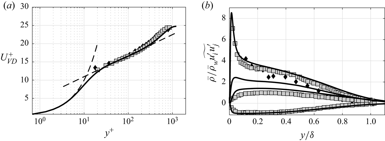
Figure 1. Comparison of (a) van Driest-transformed mean velocity profile and (b) density-scaled Reynolds stress components for the incoming boundary layer with reference experimental data. Symbols denote experiments by Elena & Lacharme (Reference Elena and Lacharme1988) (diamond,  $M_\infty = 2.32$,
  $Re_\theta = 4700$) and Piponniau et al. (Reference Piponniau, Dussauge, Debiève and Dupont2009) (squares,
  $M_\infty = 2.28$,
  $Re_\theta = 5100$).
Various studies focused on the computational analysis of the confinement effects imposed by the presence of sidewalls for STBLIs (Bermejo-Moreno et al. Reference Bermejo-Moreno, Campo, Larsson, Bodart, Helmer and Eaton2014; Poggie & Porter Reference Poggie and Porter2019; Deshpande & Poggie Reference Deshpande and Poggie2021). In particular, using wall-modelled LES with an equilibrium wall model to replicate our same reference experiment, Bermejo-Moreno et al. (Reference Bermejo-Moreno, Campo, Larsson, Bodart, Helmer and Eaton2014) found that the mean separation bubble behind the interaction is characterised by a strong three-dimensionality imposed by the lateral confinement, and observed that the size of the bubble is significantly larger than that predicted by spanwise-periodic simulations. Therefore, to compare our results with the experimental measurements, in the following we use scaled interaction coordinates,  $x^* = (x-x_0)/L_{int}$ and
  $y^* = y/L_{int}$, where
  $L_{int}$ denotes the interaction length scale, defined as the distance between the nominal impingement location and the foot of the reflected shock, and
  $x_0$ denotes the mean position of the ideal incident shock. In the reference experimental work,
  $x_0$ is equal to the mean position of the reflected shock. As a result, our values of
  $x^*$ are quantitatively different from those in Dupont et al. (Reference Dupont, Haddad and Debiève2006), even if the actual positions are correspondent. For the present DNS data, the ratio
  $L_{int}/\delta _0$ is equal to
  $3.30$, a value larger than that previously obtained at reduced Reynolds number (
 $L_{int}/\delta _0 = 2.89$) but smaller than the experimental measurement (
 $L_{int}/\delta _0 = 4.18$). Table 2 reports a comparison of the length scales obtained with some references.
Table 2. Comparison of the length scales of the STBLI considered ( $M_\infty \approx 2.28$,
  $\phi = 8^\circ$) with some references.
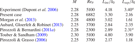
 $^{a}$Indicates that the separation length has been estimated by the relation
  $L_{sep} = 0.8\,L_{int}$ (Clemens & Narayanaswamy Reference Clemens and Narayanaswamy2009).
After an initial transient needed to develop the reflected shock and to achieve a statistically steady state, the computation was advanced, with  $U_\infty$ being the free-stream velocity, for a total time
  $T \approx 2000\,\delta_0/U_{\infty}$, which is much longer than the previous DNS simulations. It is worth highlighting that the time interval here considered allows us to cover several low-frequency cycles (approximately 25 cycles), thus making possible an in-depth analysis of the wall-pressure signature unsteadiness. The simulation time step is
  $\Delta t \approx 0.0008\,\delta _0/U_{\infty }$ and the wall-pressure history is recorded with a sampling time
  $\Delta t \approx 0.04\,\delta _0/U_{\infty }$.
A comparison of the DNS results with the PIV data measured in the reference experiment is shown in figure 2, which reports the contours of the mean streamwise velocity  $\bar{u}/U_\infty$, mean vertical velocity
  $\bar{u}/U_\infty$, streamwise velocity fluctuations
  $\bar{u}/U_\infty$, vertical velocity fluctuations
  $\bar{u}/U_\infty$, and Reynolds shear stress
  $\bar{u}/U_\infty$. In the figure, contour lines obtained from DNS are superposed onto heat maps derived from PIV in a limited region close to the interaction zone. The comparison highlights that the overall structure of the interaction is recovered effectively. The numerical simulation reproduces correctly the thickening of the upstream boundary layer and the amplification of the turbulence across the interaction, which are associated with the shedding of vortices in the shear layer developing at the separation shock. It is worth highlighting that, although a similar qualitative comparison was also previously observed at reduced Reynolds number, the present DNS results provide a better quantitative agreement with the experiment with respect to previous works, in particular with regard to the intensity of the turbulent fluctuations. Figure 3 shows an instantaneous contour of the non-dimensional temperature on a vertical slice, in which the black line indicates the locus of the points characterised by the sonic Mach number. The instantaneous separation region is highlighted by indicating the edge of the local separation bubble. From the figure, we can observe the classical structure of the STBLI. The thickening of the boundary layer, induced by the adverse pressure gradient from the shock system, makes the sweeps and ejections of the fluid towards and from the wall more evident. Moreover, the reflected shock generates an upward deflection of the flow before the virtual impingement point of the incident shock, thus promoting separation between
  $x^* = -0.5$ and
  $x^* = 0.0$. On top of the recirculation region, the innermost part of the incident shock interacts with the vorticity of the supersonic boundary layer in a non-trivial way, inducing even subsonic regions close to the intersection point between the incident and the reflected shocks. Finally, the following expansion and recompression that bring back the fluid to the original mean direction are also evident, especially in the top part of the slice.
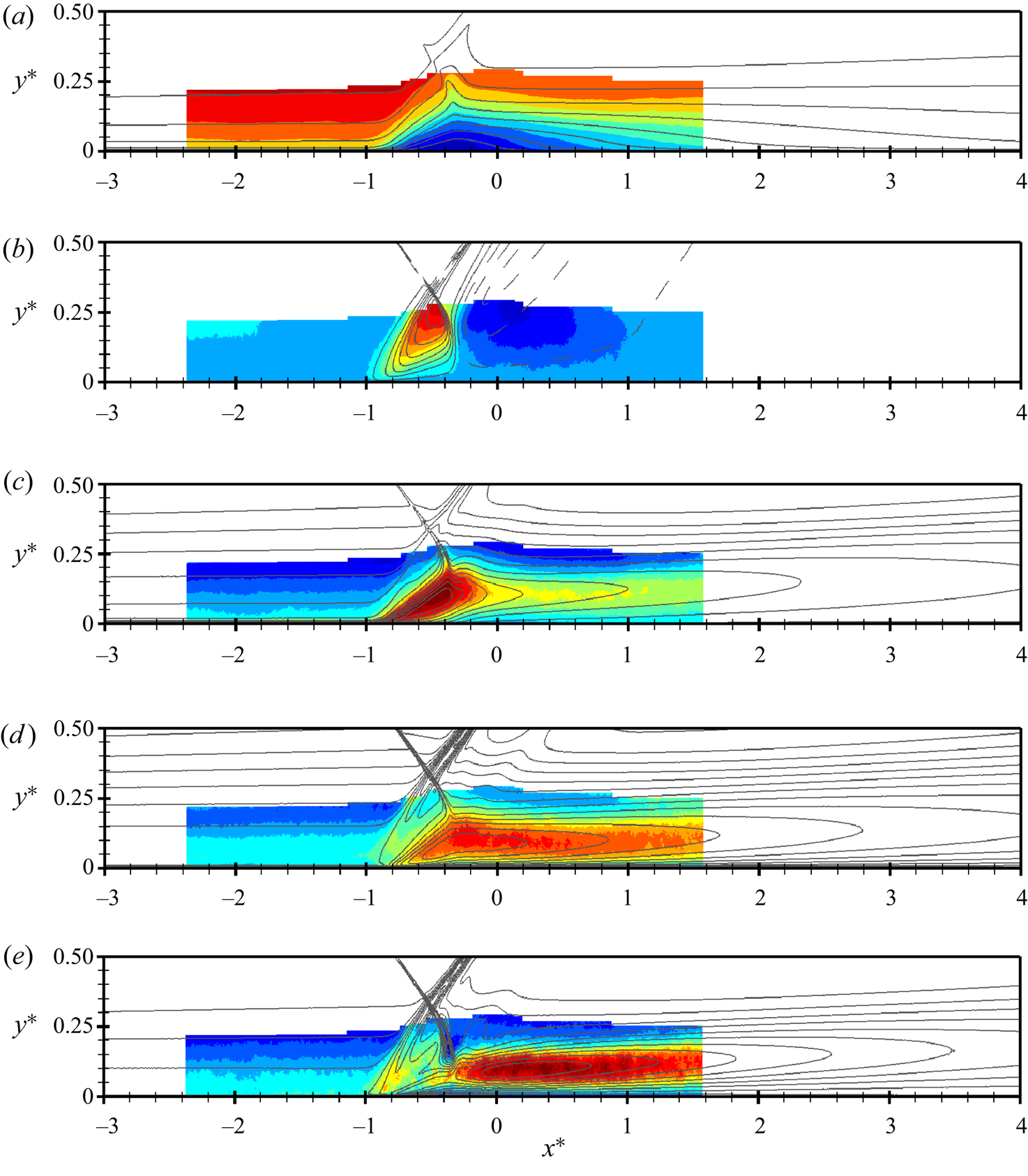
Figure 2. Comparison of velocity and Reynolds stress components on the spanwise centre plane in the interaction region. Colour maps refer to experimental PIV data, whereas DNS data are shown using contour lines. Mean streamwise velocity, mean vertical velocity, streamwise velocity fluctuations, vertical velocity fluctuations and Reynolds shear stress: (a)  $\bar {u}/U_\infty$; (b)
  $\bar {v}/U_\infty$; (c)
  $\overline {u'^2}/U_\infty ^2$; (d)
  $\overline {v'^2}/U_\infty ^2$; (e)
  $-\overline {u'v'}/U_\infty ^2$.
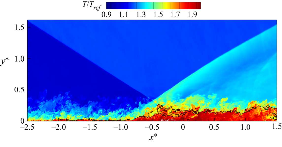
Figure 3. Instantaneous contour of the non-dimensional temperature on a vertical slice. The black line indicates the points characterised by Mach number equal to 1, whereas the white line highlights the edge of the instantaneous recirculation bubble.
4. Analysis of the results
In this section, we focus on the behaviour of the wall pressure by investigating the frequency and the intermittent content of the time signals collected around the shock region by means of classical Fourier analysis and by means of wavelet decomposition. Extracting the features of this signal means understanding the behaviour of the shock unsteadiness, which is the main responsible for the dynamics of the wall-pressure fluctuations besides turbulence. In addition, we also provide an analysis of the dynamics of the separation bubble in the time/time-scale domain, and we discuss the relationship between the unsteadiness of the shock and the motion of the recirculating region.
4.1. Time-averaged statistics of the wall pressure
At first, we focus on the behaviour of the mean pressure along the wall  $\bar{p}_w/p_\infty$, where
  $p_\infty$ is the free-stream pressure. Figure 4(a) shows the streamwise evolution of the mean wall pressure, obtained by averaging the signal in time and in the spanwise direction, together with the experimental results from the reference work (Dupont et al. Reference Dupont, Haddad and Debiève2006). Upstream of the interaction, the mean pressure is approximately constant and equal to the free-stream value. Later on, the pressure increases smoothly because of the presence of the oscillating shock, and after approximately
  $2\,L_{int}$ it reaches a plateau region. The comparison with the experimental data is satisfactory. Figure 4(b) reports instead the comparison of the streamwise distribution of the RMS of the wall pressure fluctuations
  $\sqrt{\overline{p'^2}}/p_\infty$. The typical behaviour shown in other STBLIs is observable. At first, downstream of the foot of the shock, the intensity of the fluctuations increases suddenly because of the backward and forward movement of the reflected shock. Then, in the separation and re-attachment region, the intensity decays, although the level of the fluctuations remains always higher than that of the attached boundary layer. The numerical results (solid black line) seem to show an overestimation of the fluctuation intensity, but if the r.m.s. is evaluated integrating the frequency spectra up to the cutoff of the experimental sensors (solid red line), the results agree well with the measurements.

Figure 4. Streamwise evolution of (a) mean wall pressure and (b) wall-pressure fluctuation intensity across the interaction region. Here,  $\bullet$ (green) experimental data (Dupont et al. Reference Dupont, Haddad and Debiève2006) – present DNS – (solid red line) present DNS root mean square (r.m.s.) evaluated by integrating the frequency spectra up to the cutoff of the experimental sensors: (a)
  $\bar {p}_w/p_\infty$; (b)
  $\sqrt {\overline {p'^2}}/p_\infty$.
4.2. Fourier analysis of the wall pressure
The premultiplied power spectral density (PSD) of the wall-pressure signals has been computed for positions ranging from the zone before the shock to the relaxation zone, and the results are reported in figure 5. This map reveals the frequencies that contribute the most to the global energy of the local wall-pressure fluctuations, and the characteristics that clearly emerge agree with what was shown in Dupont et al. (Reference Dupont, Haddad and Debiève2006). In order to better interpret the different regions of the interaction, we report on top of the map also the distribution of the time- and spanwise-averaged friction coefficient  $C_f = \tau _w / 1/2 \rho U_\infty ^2$, where
  $\tau _w$ is the wall shear stress. Consistently with the literature, the mean friction coefficient is characterised by the presence of two negative peaks, where the upstream one has typically a larger amplitude in absolute value. However, Morgan et al. (Reference Morgan, Duraisamy, Nguyen, Kawai and Lele2013) showed that as the Reynolds number increases, the absolute magnitude of the first negative peak of the
  $C_f$ decreases, which thus explains the distribution observed in our case leading to the appearance of two completely separate separation bubbles in the mean field. However, the behaviour observed in the mean field is actually made of the superposition of different instantaneous states, with the separation bubble alternating between a smaller and a significantly larger extent compared with what indicated by the negative mean friction coefficient. On the basis of these observations, we define as a separation length the extent that goes from the first
  $C_f$ minimum at approximately
  $x^* \approx -0.8$ to the point with null
  $C_f$ at approximately
  $x^* \approx -0.15$. A separation length of
  $L_{sep}/L_{int} \approx 0.65$ or
  $L_{sep}/\delta _0 \approx 2.16$ is finally obtained, which is in line with the trend observed in Morgan et al. (Reference Morgan, Duraisamy, Nguyen, Kawai and Lele2013) for increasing Reynolds number.

Figure 5. Friction coefficient and premultiplied power spectral density of the wall pressure along the interaction. The horizontal blue line in the first plot indicates the null value of  $C_f$, whereas the vertical dashed lines indicate the position of the probes used for the sampling of the wall-pressure signals.
The frequencies in the contour of figure 5 can be conveniently split into four separate zones, each involving its own characteristic temporal scales:
(i) the incoming turbulent boundary-layer zone,
 $x^* < -0.8$, characterised by attached flow and high-frequency contributions, with $S_L = f L_{int} / U_\infty > 1$, where f is the frequency;
(ii) the unsteady foot of the reflected shock,
$x^* \approx -0.8$, characterised by low-frequency energy content. The peak is widespread along a broad range of frequencies, suggesting an underlying shock unsteadiness more complicated than a simple periodic oscillation. In this region, the adverse pressure gradient imposed by the moving shock reduces the friction coefficient and forces the flow to start the separation;(iii) the interaction zone,
$-0.8 < x^*< -0.2$, characterised by intermediate turbulent scales developing in the detached supersonic shear layer. In this region, the spectrum reaches also its overall maximum in the point of minimal friction, which corresponds to the centre of the aft portion of the recirculation bubble;(iv) the relaxation zone,
$x^* > -0.2$, characterised by medium-frequency fluctuations developing in the separation region and dominating the boundary layer even after the reattaching point.


One of the most interesting characteristics revealed by the spectral map is the substantial distinction between the frequency content of the shock movement and the frequency content of the attached boundary layer, the separated shear layer, and the relaxation region. Figure 6 shows the premultiplied PSD in correspondence of the highlighted probes at  $x^* = -1.60$,
  $-0.79$,
  $-0.27$ and
  $0.97$ to better appreciate the spectral features of the fluctuations in points representative of the above presented zones. In particular, at
  $x^* = -0.79$, the broad and high-amplitude peak at
  $S_L \approx 0.04$ reflects the low-frequency unsteadiness of the shock motion, while the second wide bump with a peak at
  $S_L \approx 1.5$ is the trace of the incipient separated supersonic shear layer.

Figure 6. Premultiplied PSD of the wall-pressure signal at:  ${\cdot }\ {\cdot }\ {\cdot }$
  $x^* = -1.60$, - -
  $x^* = -0.79$, -
  ${\cdot }$ -
  $x^* = -0.27$, –
  $x^* = 0.97$. The vertical dashed line indicates the low-frequency peak at
  $S_L = 0.04$.
4.3. Wavelet analysis and detection of intermittency of the wall pressure
Elements of the wavelet theory can be found in several texts (Kaiser & Hudgins Reference Kaiser and Hudgins1994; Mallat Reference Mallat1999), whereas Lewalle (Reference Lewalle1994) and Farge (Reference Farge1992) discussed its applications to fluid mechanics. Here, we report few elements to clarify the following discussion.
The wavelet transform of a continuous signal  $g(t)$ is defined as
 \begin{equation} G_{\varPsi}(k,\tau) = k \int_{-\infty}^{+\infty} g(t)\varPsi^{*}(k(t-\tau))\,{\rm d}t , \end{equation}
where  $\varPsi$ is the wavelet mother function,
  $k$ is a dilatation parameter,
  $\tau$ is the time-translation parameter and
  $*$ denotes the complex conjugate. By varying the wavelet scale
  $k$ and translating along the time with the time shift
  $\tau$, one can construct a picture showing the amplitude of any feature at a certain scale and also its temporal evolution. In this study, the Morlet wavelet has been chosen since higher resolution in frequency can be achieved when compared with other mother functions. An analytical expression for the complex Morlet wavelet is
 \begin{equation} \varPsi(t) = {\rm \pi}^{{-}1/4} {\rm e}^{{\rm i} \omega_0 t} {\rm e}^{{-}t^2/2}, \end{equation}
where  $\omega _0$ is the non-dimensional frequency, which is equal to 6 here to satisfy the admissibility condition (Farge Reference Farge1992). If
  $\hat {g}(\omega )$ is the Fourier transform of
  $g(t)$
 \begin{equation} \hat{g}(\omega) = \int_{-\infty}^{+\infty} g(t) {\rm e}^{-{\rm i} \omega t} \,{\rm d}\omega, \end{equation}
then it follows that
 \begin{equation} G_{\varPsi}(k,\tau) =\frac{1}{2{\rm \pi}} \int_{-\infty}^{+\infty} \hat{g}(\omega) \hat{\varPsi}^*\left(\frac{\omega}{k}\right) {\rm e}^{{\rm i} \omega t} \,{\rm d}\omega\,. \end{equation}
As a consequence, the wavelet transform at a given scale  $k$ can be interpreted as a band-pass filter in the Fourier space. Finally, following the method of Meyers, Kelly & O'Brien (Reference Meyers, Kelly and O'Brien1993), the relationship between the equivalent Fourier period and the wavelet scale can be derived analytically by substituting a cosine wave of known frequency into (4.3) and computing the scale
  $k$ at which the wavelet power spectrum reaches its maximum. More details about the operative algorithms adopted to compute the wavelet transform in this work can be found in Torrence & Compo (Reference Torrence and Compo1998).
In the following, we apply the wavelet analysis to the wall-pressure signal at four relevant stations, respectively at  $x^* = -1.60$,
  $-0.79$,
  $-0.27$ and
  $0.97$ (see also figure 5 for the position of the numerical probes). In particular, we first focus on the regions before and in the proximity of the foot of the reflected shock; then, we address the recirculating region, and finally we consider the re-attachment location. Figure 7 presents the modulus of the Morlet transform
  $G_{\varPsi }(k,\tau )$, the so-called scalogram, of the wall-pressure signals at the four prescribed locations. The abscissa reports the non-dimensional time and the ordinate reports the temporal scale
  $k$ of the events in log scale. The blue colour indicates a small magnitude of
  $|G_{\varPsi }(k,\tau )|$, while the red colour indicates a larger wavelet modulus, representing a more intense modulation of the amplitude of the pressure fluctuations within a certain range of temporal scales
  $k$ and at the given time instant
  $\tau$. Indeed, the real part of the wavelet coefficient is proportional to the amplitude of the fluctuation (
 $p'$), while the imaginary part is proportional to its time variation (
 $\partial p'/\partial t$) (Abe, Kiya & Mochizuki Reference Abe, Kiya and Mochizuki1999). Figure 7(a) shows the modulus of the Morlet transform for the wall pressure recorded at
  $x^* = -1.60$, which is inside the boundary layer and before the foot of the reflected shock. It can be seen that, as expected, the attached boundary layer is characterised by small-scale eddies, which appear to be randomly distributed and fairly time filling, although the spotted appearance underlines the intermittent character of such turbulent structures. Figure 7(b) shows the wavelet modulus at
  $x^* = -0.79$, immediately downstream of the foot of the reflected shock. Given the position, the pressure signal from this probe is clearly modulated by the shock movement in the amplitude and in the characteristic temporal scales, or instantaneous frequencies if we consider the inverse of the temporal scales. The contour confirms that the shock movement has a dominant content at low frequencies/large time scales, as observed in the Fourier spectra. However, it reveals also that this motion is actually made of a collection of events localised in time and characterised by different temporal scales, larger than and well separated from the ones present in the upstream boundary layer. The spectral content from the Fourier analysis is thus the result of an average in time of such events, whose combined effect is the broad low-frequency peak spotted in figure 5. Figure 7(c) characterises instead the pressure signal at
  $x^* = -0.27$, in the small separated region surrounded by the detached supersonic shear layer. Here, the wavelet map is representative of a shock-induced turbulent recirculating flow: the shock footprint is well visible from the distribution in time of large-scale events, appearing and disappearing in time, but also the trace of the separated shear layer emerges from the presence of small-scale, time-filling events, similarly to the region of the upstream boundary layer. Finally, figure 7(d) shows the wavelet map at
  $x^*=0.97$, the re-attachment location. Large-scale events are now more sparse, indicating that the effect of the shock unsteadiness is weaker and a new attached boundary layer is developing.

Figure 7. Wall-pressure signal and corresponding Morlet wavelet transform modulus  $|G_{\Psi}(k,\tau)|$ at (a)
  $x^* = -1.60$, (b)
  $x^* = -0.79$, (c)
  $x^* = -0.27$, (d)
  $x^* = 0.97$. For each probe, only values of the coefficients above 30 % of the relative maximum are shown.
The scalograms shown above reveal the presence of different events, or structures, at various scales, and allows us to detect their degree of intermittency. In this context, we define the intermittency as the alternation of regimes with normal spectral content and regimes with significant excess – or burst – of energy in a given range of scales. Given the wavelet transform coefficients  $G_{\varPsi }(k,\tau )$, it is possible to obtain the scale-time distribution of the energy density
  $|G_{\varPsi }(k,\tau )|^2$ of the wall-pressure signal
  $p(t)$ at specified scale
  $k$ and time
  $\tau$. Taking into account this property, Meneveau (Reference Meneveau1991) and Camussi & Bogey (Reference Camussi and Bogey2021) suggested that an effective indicator of the intermittency is the squared local intermittency measure, denoted as
  $LIM2$
 \begin{equation} LIM2(k,\tau)=\frac{|G_{\varPsi}(k,\tau)|^4}{\langle|G_{\varPsi}(k,\tau)|^2\rangle_{\tau}^2}, \end{equation}
where  $\langle \bullet \rangle _\tau$ indicates the time average of the considered quantity. The rationale for this statement lies in the fact that
  $LIM2$ can be interpreted as a time-scale-dependent measure of the flatness factor or kurtosis of the input signal
  $g(t)$, which indicates the importance of rare events for the probability distribution of the variable and is defined as the Pearson's index
 \begin{equation} FF=\frac{\langle g^{'4} \rangle}{\langle g^{'2}\rangle^2} , \end{equation}
where  $g'$ is the fluctuating part of
  $g$, and
  $\langle \bullet \rangle$ indicates the expected value of the considered quantity. Therefore, the
  $LIM2$ parameter will be equal to 3 when the probability distribution is Gaussian, while the condition
  $LIM2>3$ identifies only those rare outliers contributing to the deviation of the wavelet coefficients from a normal, Gaussian distribution. According to Camussi & Bogey (Reference Camussi and Bogey2021), the energy increment at a certain scale
  $k$ and time
  $\tau$ is associated with the passage of a coherent structure characterised by the scale
  $k$.
$k$.
Figure 8(b) shows the  $LIM2$ field for the signal at
  $x^*=-0.79$, which has a general kurtosis (see (4.6)) equal to 3.20. Only the levels greater than the threshold value 3 are shown. In this picture, one can observe the occurrence of the intermittent events in the time-scale region characterising the shock unsteadiness (indicated in grey in the background), which is the range of large temporal scales defining the broad low-frequency peak in the Fourier spectrum (see figure 6). Now the significant energy bursts appear more sparse in time with respect to the representation offered in figure 7(b). In addition, we can also see the intermittency of the turbulent content at smaller temporal scales. Moreover, we notice that the rather long period considered for the simulation we carried out is able to capture only few coherent intermittent events at large time scales. For this reason, it is evident that, to characterise thoroughly the unsteadiness of STBLI, very long periods must be considered, in order to deconstruct the broadband low-frequency unsteadiness reported in the literature into the actual scattered dynamics associated with the flow.

Figure 8. (a) The green curve reports the original wall-pressure signal at  $x^* = -0.79$, while the black curve reports its filtered-and-reconstructed part. (b) The p.d.f. of the original signal with the corresponding fitted normal distribution in grey. (c) Contour of
  $LIM2$ of
  $p_w/p_\infty$. Values below 3 are cut off, whereas the grey area indicates the scales used for the filtering procedure. (d) The corresponding wavelet flatness factor (WFF). The horizontal dashed lines indicate the peak low frequency.
A sign of the presence of intermittent events is already evident from the probability density function (p.d.f.) of the signal (top right), which shows a distribution slightly departing from a normal Gaussian function in its external parts. However, although classical statistical indicators suggest the relevance of outlier events with large deviation from the mean, as indicated by the mildly non-Gaussian p.d.f. and kurtosis of the signal, they are not able to locate and estimate precisely the single intermittent episodes, which thus makes it hard to understand the physical mechanisms behind the resulting dynamics. The  $LIM2$ measure instead allows one to spot the instants and the scales of data that differ significantly from other observations, and thus makes it possible to characterise more accurately the dynamics of the flow, which may be hidden in time-averaged analyses.
After the inspection of such a scenario, we propose the following procedure to extract the characteristics of the signal of interest (Consolini & De Michelis Reference Consolini and De Michelis2005): first, we filter the original wall-pressure using (4.4), considering only the wavelet coefficients of the large scales associated with the low-frequency shock unsteadiness (grey region in the  $LIM2$ contour); then, we reconstruct the intermittent signal
  $p_{w,I}$ only on the basis of the wavelet coefficients related to the burst events by means of the conditioned inverse continuous wavelet transform
 \begin{equation} p_{w,I}(k_{min}, t)=\frac{1}{C_{\varPsi}} \int_{k_{min}}^{\infty} {\rm d}k \int_{-\infty}^{\infty} G_{\varPsi,LIM2}(k,\tau)\varPsi\left(\frac{\tau-t}{k}\right){\rm d}\tau, \end{equation}
where  $C_{\varPsi }$ is a normalisation constant depending on the chosen wavelet,
  $k_{min}$ is the smallest time scale considered by the large-scale-pass filtering and
  $G_{\varPsi,LIM2}(k,\tau )$ are the wavelet coefficients related to the intermittent events, extracted using the
  $LIM2$ condition (
 $LIM2(k,\tau ) > 3$). This procedure can be considered as an extension of the one adopted by Poggie & Smits (Reference Poggie and Smits1997), in which the authors used the extremes in the global wavelet spectrum to filter the signal in the space of the wavelet temporal scales. Figure 8(a,b) shows the original wall pressure in time at the foot of the reflected shock (green line) together with its filtered-and-reconstructed intermittent part (black line). The inspection of the reconstructed signal allows us to appreciate that the small-scale turbulent fluctuations have been removed by the procedure, and that only the pattern given by the events associated with the shock intermittency remains. Therefore, it is possible to detect the signal shape given by the movement of the shock, which is governed by a predominantly two-dimensional mechanism (high spanwise coherence) according to Sasaki et al. (Reference Sasaki, Barros, Cavalieri and Larchevêque2021).
The  $LIM2$ map can be averaged in time to recover the flatness factor as a function of the temporal scale (Camussi & Bogey Reference Camussi and Bogey2021), and thus to reveal the most intermittent temporal scales. This quantity is usually called wavelet flatness factor (WFF) and is defined as
 \begin{equation} WFF(k)=\langle LIM2(k,\tau)\rangle_{\tau}=\frac{\langle|G_{\varPsi}(k,\tau)|^4\rangle_{\tau}}{\langle|G_{\varPsi}(k,\tau)|^2\rangle_{\tau}^2}\,. \end{equation}
Figure 8(d) shows the WFF for the corresponding  $LIM2$ map of the wall pressure at the shock foot. We can see that the WFF is characterised by two peaks at large scales, one at
  $k\,U_\infty /L_{int} \approx$ 15 and the other at
  $k\,U_\infty /L_{int} \approx$ 36. However, the peak frequency computed by the Fourier and wavelet spectra lies in between the scales indicated by the WWF, at
  $S_L = 0.04$ or
  $k\,U_\infty /L_{int} = 24.27$. This result represents an indication that the most probable temporal scales of intermittency are different from the most probable temporal scales of the overall unsteadiness.
4.4. Wavelet intermittency analysis of the separation bubble dynamics
In view of the many works sustaining that the low-frequency shock motion is strictly related to the dynamics of the separation bubble (Dupont et al. Reference Dupont, Haddad and Debiève2006; Piponniau et al. Reference Piponniau, Dussauge, Debiève and Dupont2009; Pasquariello et al. Reference Pasquariello, Hickel and Adams2017), we then attempt to relate the behaviour of the wall pressure at the foot of the shock to the change in time of the separation region, to assess the eventual correspondence between these two features and in the attempt of providing a characterisation of their link locally in time and time scale. In fact, Piponniau et al. (Reference Piponniau, Dussauge, Debiève and Dupont2009) highlighted that, far from weak interactions with incipient separation, where there seems to be an actual correlation (Humble et al. Reference Humble, Elsinga, Scarano and van Oudheusden2007), and at least for the case of shock reflections, there is no relevant coherence between the upstream superstructures and the dynamic response of the system as suggested by Ganapathisubramani, Clemens & Dolling (Reference Ganapathisubramani, Clemens and Dolling2007). Therefore, for the case under consideration, the dynamics of the separated bubble seems clearly the main source of the low-frequency unsteadiness.
In order to detect the zone occupied by the recirculating flow, we recorded the whole area occupied by negative streamwise velocity at each instant, assuming that this provides a rough estimate of the extent of the bubble. The time signal of such area, indicated with  $A_{u<0}/A_{ref}$, is reported in figure 9(a,b) together with its corresponding filtered-and-reconstructed part. On the right, we report also the p.d.f. of the original signal which has a kurtosis equal to 3.68. The extent of the separation bubble oscillates between two more probable values but presents also many sudden variations at larger areas. The p.d.f. thus reports a highly skewed, bimodal distribution with a long tail that reveals the presence of important and intermittent fluctuations in the breathing motion of the separation area. Contours of the Mach number for two different states during an intermittent event are also shown in figure 10, in which the points with null streamwise velocity are indicated with a white line that gives a hint of the area
  $A_{u<0}$. In the first state, the flow is largely separated, and the deviation imposed on the flow by the presence of the separation bubble is significant. On the other hand, in the second state, the flow is almost completely attached, and the deviation is practically negligible. (A movie of the time evolution of the contour of the Mach number on a vertical slice during the intermittent event around
  $t\,U_\infty /\delta _0 \approx 1160$ is provided in the supplementary movie available at https://doi.org/10.1017/jfm.2022.1038.) In order to analyse and compare the intermittency of the wall pressure induced by the oscillation of the shock and of the fluctuations of the separation extent, we report a contour of the
  $LIM2$ measure also for
  $A_{u<0}$ (figure 9c,d). From the comparison with figure 8, we can observe that some of the most important events of the
  $LIM2$ of the wall pressure at the shock foot correspond to the most important events of the corresponding measure of the separation bubble (see for example
  $t U_\infty / \delta _0 \approx 200$,
  $1160$, and
  $1380$), even though the temporal scales are different. The situation is even more evident when we look at figure 11, which reports the time evolution of the
  $LIM2$ intermittency measure averaged in scale, considering only the large-scale interval that characterises the low-frequency unsteadiness. The intermittency of the pulsation of the separation bubble is thus transmitted to the unsteadiness of the shock system, and thus to its wall-pressure signature at the wall, or vice versa. However, although many of the intermittent events of the wall pressure have a corresponding trace in the
  $LIM2$ measure of the separation bubble area, other energy bursts for the wall pressure do not seem to have a direct relation with the breathing mode of the system, e.g.
  $t U_\infty / \delta _0 \approx 485$,
  $887$, or
  $1270$. This observation suggests that the low-frequency, intermittent unsteadiness of the shock can only be in part related to the breathing motion of the separation bubble, and so that other key actors may play a role in this phenomenon.

Figure 9. (a) The green curve reports the original  $A_{u<0}/A_{ref}$ signal, while the black curve reports its filtered-and-reconstructed part. (b) The p.d.f. of the original signal. The two peaks of the distribution are indicated with grey dotted lines. (c) A contour of
  $LIM2$ of
  $A_{u<0}/A_{ref}$. Values below 3 are cut off, whereas the grey area indicates the scales used for the filtering procedure. (d) The corresponding WFF.

Figure 10. Instantaneous contours of the Mach number on a vertical slice for two different states during the intermittent event around  $t \, U_\infty / \delta _0 \approx 1160$. The white line indicates the points with null streamwise velocity. (a)
  $t \, U_\infty / \delta_0 = 1158.1$, the area occupied by the bubble is large; (b)
  $t \, U_\infty / \delta_0 = 1195.6$, the bubble is almost absent.

Figure 11. Normalised scale average of the  $LIM2$ measure above threshold value 3, considering only the large scales – low frequencies – used for the filtering procedure. – Wall-pressure signal at the shock foot, - - separation bubble area signal.
Finally, if we observe also the WFF of the area signal (figure 9d), we can see that the distribution of the flatness factor along the time scales follows closely the behaviour of the WFF of the wall pressure (figure 8d). As a result, also for the dynamics of the separation bubble extent, the most probable intermittent scales are different from the large temporal scales characterising the overall shock unsteadiness (the broad low-frequency peak in the Fourier domain).
In order to further characterise the relationship between the signals of the wall pressure at the foot of the shock and the separation area, we consider also the information from the wavelet cross-spectrum and from the wavelet coherence (Torrence & Webster Reference Torrence and Webster1999; Grinsted, Moore & Jevrejeva Reference Grinsted, Moore and Jevrejeva2004; Maraun, Kurths & Holschneider Reference Maraun, Kurths and Holschneider2007). Through such analyses, we are able to determine whether there are regions in the time/time-scale domain with large common power and also if these have consistent phase relationship, which could potentially suggest the causality between the two time series. In particular, the wavelet cross-spectrum of two time series  $x$ and
  $y$, with wavelet transform
  $G_\varPsi ^{x}$ and
  $G_\varPsi ^{y}$, respectively, is defined as
 \begin{equation} G_{x,y} (k, \tau) = G_\varPsi^{x} \left(G_\varPsi^{y}\right)^*, \end{equation}
with  $*$ indicating the complex conjugation. The wavelet cross-spectrum represents thus the covarying power of the two processes. This means that an independent variance appearing only in one of the two single spectra does not appear in the cross-spectrum, and that the cross-spectrum vanishes for independent processes. Moreover, for the related time and time scales, the complex argument of the wavelet cross-spectrum
  $\phi (G_{x,y})$ gives an indication of the local relative phase between the original time series in the time/time-scale domain. For example, to establish a simple cause and effect relationship between two phenomena represented by the two time series, oscillations are expected to be locked in phase in the regions with significant common power (Grinsted et al. Reference Grinsted, Moore and Jevrejeva2004). Moreover, starting from the definition of the wavelet cross-spectrum, it is possible to define a direct measure of the correlation between two signals throughout the time and the scales. Torrence & Webster (Reference Torrence and Webster1999) defined the so-called wavelet coherence
  $R^2_{x,y}$ between two time series
  $x$ and
  $y$ as
 \begin{equation} R^2_{x,y} (k, \tau) = \frac{|S(G_{x,y})|^2}{S(|G_\varPsi^x|^2) S(|G_\varPsi^y|^2)}, \end{equation}
where  $S$ is a smoothing operator in time and time scale. The wavelet coherence has values between zero and one, and has the relevant property of quantifying the linear relationship between two processes (Maraun et al. Reference Maraun, Kurths and Holschneider2007). Figure 12 shows the wavelet coherence between the signal of the wall pressure at the foot of the shock and that of the separation area. In the first instance, we consider the original signals (figure 12a). At small time scales, the turbulent fluctuations result in the typical pattern with long, intermittent, vertical strikes covering the high-frequency range. The coherence is here mostly related to the properties of the small turbulent coherent structures. In the large-scale – low-frequency – range, large areas of the contour show that the two signals present a significant instantaneous correlation, although they are not phase locked. However, the distribution of the peak regions seems to contradict the correspondence of the intermittent events inferred from the comparison of the
  $LIM2$ measure of the two signals (figures 8–9). For this reason, we consider also the wavelet coherence of the two signals filtered and reconstructed according to the procedure proposed above (figure 12b). Given the large-scale-pass preliminary filtering of the signal, the small time-scale region is not considered. From the figure, we can observe an important coherence with strong events sparse in time, and most of all, we can recognise the trace of the most important intermittent events pointed by the
  $LIM2$ comparison previously discussed. The signal processing isolates the intermittent content of the signal, and the wavelet coherence analysis allows us to reveal that the intermittency of the wall pressure at the foot of the shock is strictly related to the pulsation of the separation area. However, if we look at the phase angle of the cross-wavelet between the filtered-and-reconstructed signals in figure 13 for the most coherent events, we can see that also for the intermittent signals the phase does not remain constant across the time scales, indicating that a simple linear relationship between the intermittency of the breathing mode and that of the unsteadiness of the shock cannot be inferred.

Figure 12. Wavelet coherence between the shock foot wall-pressure signal and the separation area. Shaded region in the right contour is not significant given the preliminary large-scale-pass filtering. (a) Original signals. (b) Intermittent signals.

Figure 13. Cross-wavelet phase angle for times and time scales for which the wavelet coherence between the filtered wall pressure and separation area is larger than 0.6.
5. Conclusions
The present work analyses the wall-pressure fluctuations of the STBLI generated by an impinging oblique shock wave, by leveraging the enhanced capabilities of the wavelet analysis in the time/time-scale domain (Mallat Reference Mallat1999).
The data are obtained numerically by means of a DNS carried out at moderate Reynolds number, so that the shock is able to penetrate into the turbulent boundary layer, leaving a marked trace in the wall-pressure signal that makes it possible to examine the shock unsteadiness and its intermittency more adequately than in the cases with lower Reynolds number (Pirozzoli Reference Pirozzoli2011).
Although the classical Fourier analysis provides useful information about the spectral content of the overall STBLI unsteadiness, other techniques may be better able to analyse the transient phenomena that are taking place. Among them, given its compact support, the wavelet transform represents a valuable tool that is still scarcely used in flows similar to the one considered here. From the analysis of the wall-pressure signals and of the time evolution of the separation bubble, we attest in this work the ability of wavelet analysis to infer relevant information about the dynamics of STBLI.
In the first place, the validation of our results in terms of basic statistics of the fluid field and of the wall pressure shows a notable improvement in the reproduction of the reference experiment with respect to previous works. Furthermore, the analysis of the wavelet transform modulus reveals and clarifies that the broadband low-frequency peak, usually observed in the Fourier spectrum at the foot of the reflected shock in STBLIs (Clemens & Narayanaswamy Reference Clemens and Narayanaswamy2014), is actually the result of a collection of sparse, intermittent events with different temporal scales. The Fourier spectral analysis shows thus only the time-averaged effect of such behaviour and is not able to characterise the local modulation of the pressure fluctuation, which makes it impossible to understand precisely what is happening in the fluid flow correspondingly.
Then, we show that it is possible to characterise the energy and timing of the intermittent events linked to the shock unsteadiness on the basis of a wavelet-based local flatness factor, called  $LIM2$ (Meneveau Reference Meneveau1991; Camussi & Bogey Reference Camussi and Bogey2021). The global kurtosis of the wall pressure, related to the outliers in the shock signature, is thus decomposed into its evolution in the time/time-scale domain, to localise the most significant bursts of energy in the signal. Inspired by the work of Poggie & Smits (Reference Poggie and Smits1997), the identification of the frequency content characterising the shock unsteadiness and the application of the
  $LIM2$ condition have thus been used to propose a signal processing procedure to, first, separate the footprint of the shock motion from the turbulent pressure fluctuations, and then, isolate its intermittent content. The analysis of the obtained signal reveals that the intermittency of the wall pressure is mostly characterised by temporal scales that are different from those that dominate the overall unsteadiness of the shock system according to Fourier analysis.
The proposed signal processing can represent a preliminary practice for further investigations into the causality and the features of the low-frequency unsteadiness of STBLI systems, by using for example conditional statistics based on the system intermittency. In this kind of study, an essential step is in fact the proper estimation of the correlation between the motion of the reflected shock and the characteristic time scales of the incoming turbulent boundary layer, the separated region and the re-attachment region: isolating the low-frequency intermittent part of the associated time series could help recognising relations that may be overshadowed by the combination of the different components of the complete signals.
Motivated by the many studies in the literature that attest a relationship between the unsteadiness of the shock and the pulsation of the separation bubble (Piponniau et al. Reference Piponniau, Dussauge, Debiève and Dupont2009), we decided to study by means of the proposed procedure the dynamics of the recirculation region behind the reflected shock. The time signal recording the evolution of the separation bubble extent presents a skewed probability distribution with strong fluctuations between states with large and minimal separation, respectively. The analysis of the intermittency through wavelet transform shows that also the motion of the bubble has strong, sparse energy bursts at large time scales and reveals a connection between such events and those highlighted by the  $LIM2$ measure of the shock foot wall pressure, although it was not possible to estimate the statistics of such events because of the insufficient number of occurrences. In order to qualify and quantify the connection between the two signals, wavelet cross-spectra and wavelet coherence (Torrence & Webster Reference Torrence and Webster1999) have been considered for the signals processed by the proposed procedure. The study of the coherence among the times and time scales confirms that the intermittent contributions of the breathing bubble motion and the shock foot wall-pressure are highly correlated during the most important intermittent events. However, the corresponding cross-wavelet phase angle shows that there is not a simple linear relationship between the two signals, which would have suggested a causality relation similarly to what recently considered by Sasaki et al. (Reference Sasaki, Barros, Cavalieri and Larchevêque2021).
In the end, our results confirm the hypothesis about the link between the low-frequency shock unsteadiness and the breathing mode of the separation bubble, even if our investigation points out the complexity of the breathing motion and indicates that other phenomena may contribute to the dynamics of the overall system.
Supplementary movie
Supplementary movie is available at https://doi.org/10.1017/jfm.2022.1038. A movie of the time evolution of a contour of the Mach number on a vertical slice, during the intermittent event around  $t \, U_\infty / \delta _0 \approx 1160$ is available. The white line indicates the locus of the points with null streamline velocity.
Acknowledgements
We acknowledge CINECA for the availability of high performance computing resources and support during the pre-production stage of Marconi100 cluster. We also acknowledge Professor S. Piponniau and Professor P. Dupont for having provided us with the experimental data used in the validation section.
Funding
This research received no specific grant from any funding agency, commercial or not-for-profit sectors.
Declaration of interests
The authors report no conflict of interest.
Data availability statement
The full data set of the DNS simulations is of the order of thousands of gigabytes. By contacting the authors, a smaller subset can be made available.


 Open access