


1 Introduction and background
A thorough understanding of the transition from laminar to turbulent flow is needed before control strategies can be developed to facilitate natural and hybrid laminar flow. The advantage of maintaining the latter is mostly the reduction of the skin friction drag on aircraft wings and fuselage, and the potential to minimise fuel burn and pollutant emission. However, many processes affect the laminar/turbulent transition; these are not yet fully understood. A particular challenge is represented by the receptivity; the process by which natural or man-made disturbances interact and penetrate the boundary layer, exciting the flow instabilities (Morkovin Reference Morkovin1969). Herein, we focus on the receptivity of boundary layers to an acoustic field and two-dimensional roughness. In the presence of a free-stream oscillatory component (usually due to an acoustic field), the flow develops a Stokes layer (SL), which is superimposed on the T–S wave excited by the receptivity process. Given that the amplitude of the T–S wave and that of the SL are of the same order, and occur at the same frequency (i.e. acoustic oscillation), it is difficult, experimentally, to isolate the receptivity of the boundary layer. Previous experimental work has used a variety of approaches; however, these are short of ideal (Monschke, Kuester & White Reference Monschke, Kuester and White2016). Saric (Reference Saric1994) employed a complex plane technique to measure the receptivity coefficients. This technique relied on the notion that the wavelength of the sound wave is orders of magnitude larger than that of the T–S wave; therefore, the SL has a constant phase over one T–S wavelength. By employing Fourier analysis and monitoring the imaginary and real components in the complex plane, the T–S amplitude can be deduced. The drawbacks of this technique include requiring measurements at several streamwise locations (across one T–S wavelength), and the possible generation of complex acoustic fields in the tunnel’s test section (due to the continuous nature of the forcing). White, Saric & Radeztsky (Reference White, Saric and Radeztsky2000) applied a pulsed-sound technique, based on group velocities of the two types of wave field (acoustic and T–S), which are very different. With the acoustic forcing applied in short bursts, the T–S wave component is measured after a short transient (proportional to the speed of sound at which the SL travels). This technique requires a prohibitive number of ensemble averages (i.e. long acquisition time), and has inherently poor frequency resolution. Monschke et al. (Reference Monschke, Kuester and White2016) proposed a methodology that stands on the biorthogonal properties of a modified Orr–Sommerfeld equation in combination with an active control technique. This employs two secondary speakers downstream from the model to counteract possible acoustic reflections. This sophisticated approach only requires one boundary layer profile; however, this comes at the cost of significant complications with (i) the processing of the data due to the modal decomposition, (ii) the need for an active control technique, and (iii) the experimental complexity and costs (several acoustic drivers are required). Another simple and effective technique to measure the T–S component created by the roughness in isolation is to compensate for any other effects by acquiring reference data in the absence of the said roughness (Zhou, Liu & Blackwelder Reference Zhou, Liu and Blackwelder1994). This needs to be removable and, therefore, adhesive tape is commonly used. This technique, although effective, has several limitations: (i) it only allows measurements at a single positive height (i.e. protuberance), and (ii) it requires the wind tunnel to be stopped between runs to allow for the application of the tape. This procedure inherently introduces measuring uncertainties in matching the tunnel conditions; these are often of the same order of the small amplitudes one is trying to measure. Therefore, only significant heights (i.e. within nonlinear regime) can be measured with sufficient signal-to-noise ratio.
Here, we present an improved methodology based on the framework laid out in Zhou et al. (Reference Zhou, Liu and Blackwelder1994), but with the addition of dynamic adaptation of roughness height, which allows reliable measurements of the acoustic receptivity of two-dimensional boundary layers in the presence of the localised surface roughness, bypassing some of the limitations of the previous work. This novel experimental technique, based on a retracting roughness, not only provides high-quality acoustic receptivity measurements but also allows for the effect of both positive protuberances and cavities to be considered. There has also been a substantial amount of numerical work on receptivity; however, this has parted from the roughness geometry considered here (two-dimensional roughness strips arranged perpendicularly to the flow direction). De Tullio & Ruban (Reference De Tullio and Ruban2015) focused on the linear receptivity of two-dimensional boundary layers due to the interaction of acoustic disturbances and a small isolated hemispherical roughness element; asymptotic theory and direct numerical simulation (DNS) were shown to be in good agreement. Two- and three-dimensional wavy walls and non-localised roughness were investigated by Wiegel & Wlezien (Reference Wiegel and Wlezien1993), Goldstein (Reference Goldstein2014) and King & Breuer (Reference King and Breuer2001), respectively; whilst Crouch (Reference Crouch1992) and Würz et al. (Reference Würz, Herr, Wörner, Rist, Wagner and Kachanov2003) adopted localised surface imperfections. Choudhari & Streett (Reference Choudhari and Streett1992) and Airiau (Reference Airiau2000) considered the effect of suction and blowing. Other work has focused predominately on the leading-edge receptivity (Lin, Reed & Saric Reference Lin, Reed and Saric1992; Hammerton & Kerschen Reference Hammerton and Kerschen1996), which is here neglected as its effect is much weaker compared to surface roughness mechanisms (Raposo, Mughal & Ashworth Reference Raposo, Mughal and Ashworth2018). Advances in numerical techniques and a discussion of each approach are highlighted in Raposo et al. (Reference Raposo, Mughal and Ashworth2018); however, the current focus is on the physical testing. Hence, this topic is omitted.
2 Experimental facility and details
2.1 Experimental facility and model
Experiments were carried out in the closed-circuit ‘Gaster low-turbulence wind tunnel’ at City, University of London. The turbulence intensity,  $Tu$, measured in the empty tunnel, was less than
  $0.006\,\%$ of the free-stream velocity,
  $U_{\infty }$, within the frequency range 4 Hz–4 kHz at
  $U_{\infty }=18.42~\text{m}~\text{s}^{-1}$, the tunnel speed used in this study. The tunnel test section measures
  $0.91~\text{m}\times 0.91~\text{m}\times 1.82~\text{m}$ and is equipped with a 3-axis traverse system capable of reaching the streamwise location
  $x=1320~\text{mm}$. A highly polished
  $1.8~\text{m}$ long flat plate, with a span of
  $0.91~\text{m}$, and a thickness of
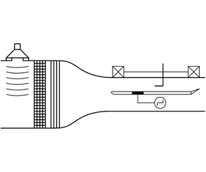
  $9.5~\text{mm}$ was mounted vertically in the test section (as shown in figure 1). The plate has a cutout that allows different rigs to be mounted at specific locations; the impact of which is further discussed in § 2.2. The elliptical leading edge (
 $20\,:\,1$ modified ellipse) manages the initial pressure gradient to sustain a laminar boundary layer. A combination of trailing edge flap and tab (which extended the plate to a total chord length of
  $2.4~\text{m}$) were used to adjust the stagnation point location, whilst the flow was forced to turbulence on the reverse side of the plate at
  $8\,\%$ chord to fix transition in order to stabilise the circulation around the plate. Base flow validation and Blasius comparison are here omitted; however, the reader is referred to figures 2.3 and 2.4 in Veerasamy (Reference Veerasamy2019) for typical accuracy achieved in this facility. Mean flow profiles are measured to estimate the virtual origin of the Blasius boundary layer profile; this is then used to correct all chordwise locations.
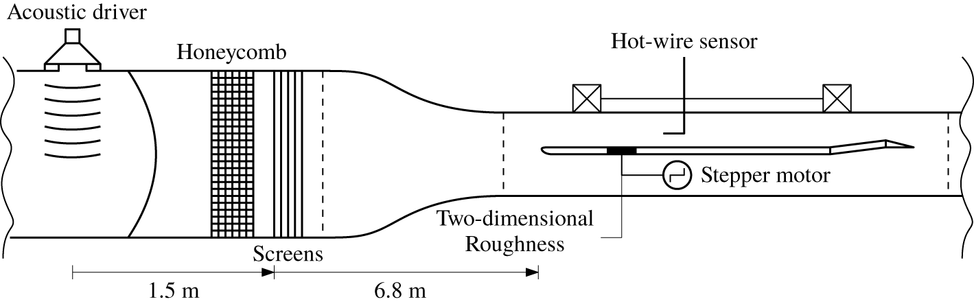
Figure 1. Wind tunnel set-up (plan view). The flow is left to right. Figure not to scale.
2.2 Roughness geometry and acoustic forcing details
It has been shown how the receptivity of the laminar boundary layer to acoustic waves is created by the presence of discrete roughness, which enables coupling of the long-wavelength acoustic disturbance with the much shorter wavelength of the T–S wave (Goldstein Reference Goldstein1983). Therefore, roughness was used in combination with sound to generate T–S waves, as in previous experimental work (Saric Reference Saric1994; Zhou et al. Reference Zhou, Liu and Blackwelder1994). A high-aspect-ratio ( $20\,:\,1$) leading-edge profile is used to minimise the leading-edge receptivity of the boundary layer so that the roughness receptivity should be dominant (Saric Reference Saric1994). The optimal roughness strip location to yield maximum disturbance amplitude at the most downstream location (i.e.
  $x=1320~\text{mm}$) was
  $570~\text{mm}$ from the leading edge (Raposo, personal communication), so that the upstream edge of the rectangular element is characterised by a Reynolds number
  $Re_{x}=(U_{\infty }x/\unicode[STIX]{x1D708})^{1/2}\approx 823$, where
  $\unicode[STIX]{x1D708}$ is the kinematic viscosity of the fluid. This is as close as possible (within the existing experimental model constraints) to the location of Branch I. The roughness location is hereafter referred to as
  $L$. The optimal width, from the receptivity perspective, is one half of the wavelength of the most amplified T–S wave (Goldstein Reference Goldstein1983), and it was calculated to be
  $28~\text{mm}$. A narrower width of
  $20~\text{mm}$ was, however, chosen for practical reasons concerning the design of the experimental rig. With this modification, it was calculated that the T–S amplitude would only be reduced in magnitude by
  $10\,\%$ compared to its optimal location (Raposo, personal communication). The roughness strip measured
  $200~\text{mm}$ across the span and presented reasonably sharp edges. This strip was embedded within an insert, which was mounted flush with the surface of the plate, as shown in figure 2(a). A total of 18 different roughness heights were used from
  $30~\unicode[STIX]{x03BC}\text{m}<|h|<750~\unicode[STIX]{x03BC}\text{m}$ (
 $0.025<|h|/\unicode[STIX]{x1D6FF}_{B}^{\ast }<0.630$). These were chosen to cover both the linear and the nonlinear amplitude forcing (Saric Reference Saric1994; Raposo et al. Reference Raposo, Mughal and Ashworth2018). The minimum height needed to generate reliable and measurable disturbances was found to be approximately
  $30~\unicode[STIX]{x03BC}\text{m}$. Table 1 summarises the test matrix and all the relevant parameters. Following Saric (Reference Saric1994), we report the three different non-dimensional numbers characterising the roughness height,
  $Re_{\infty }=U_{\infty }h/\unicode[STIX]{x1D708}$,
  $Re_{h}=U(h)h/\unicode[STIX]{x1D708}$, and
  $h^{+}=hu_{\unicode[STIX]{x1D70F}}/\unicode[STIX]{x1D708}$. These are the Reynolds number based on the free-stream velocity, the Reynolds number based on the velocity at roughness height,
  $U(h)$, and the roughness height in wall-units, respectively. The measured velocity profile was extrapolated downward linearly onto the wall from the first measurement point, satisfying the no-slip condition; the calculation of the local Reynolds numbers makes use of this linear part of the velocity profile, as in Saric (Reference Saric1994). Relative roughness heights to the unperturbed Blasius profile (with subscript
  $_{B}$) at the strip location are also included in table 1.
Table 1. Summary of test cases, measurement stations and roughness parameters.

The acoustic forcing was provided by one woofer of diameter  $370~\text{mm}$ located upstream of the contraction and flow conditioners, as indicated in figure 1. Different speaker orientations were tried with no discernible effect on the plane waves impinging on the model (i.e. uniform velocity fluctuations and phase across the span of the model). It was decided to mount the driver flush with the tunnel walls to minimise any aerodynamic disturbance. The acoustic driver was driven by a sinusoidal signal, with a frequency of
  $f_{exc}=90~\text{Hz}$, and an amplifier (Cambridge Audio TOPAZ AM1). This yields a non-dimensional frequency
  $F=([2\unicode[STIX]{x03C0}f_{exc}\unicode[STIX]{x1D708}]/{U_{\infty }}^{2})\times 10^{6}\approx 25.85$. The sound pressure level (SPL) in the test section, which was constantly monitored during tests, was chosen to maximise the receptivity process, whilst preventing nonlinear effects. This was limited to
  $80~\text{dB}$, when calculated with a customarily reference pressure of
  $20~\unicode[STIX]{x03BC}\text{Pa}$. Sensitivity tests on the T–S amplitude were conducted with respect to forcing frequency (
 $\pm 5\,\%$) and SPL. Variations of the excitation frequency produced minimal effects where disturbance amplitudes were within experimental uncertainty, whilst the boundary layer response was confirmed to scale linearly with the SPL (see the Appendix and Saric (Reference Saric1994)).
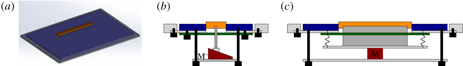
Figure 2. (a) Schematic of the insert plate (blue) with roughness strip (orange). (b) Schematic of the computer-controlled height adjustment system (side view) and (c) front view. Additional highlighted components: seal (green), wedge (red), stepper motor (M), knife-edge (dark grey).
The presence of an acoustic exciter introduces vibrations in the tunnel environment, which can also lead to the excitation of T–S waves. However, the amplitude of these undesired T–S waves due to vibrational receptivity is at least one order of magnitude lower than that of T–S waves created by acoustic forcing (Würz et al. Reference Würz, Herr, Wörner, Rist, Wagner and Kachanov2003). To ensure that the speaker did not transfer any mechanical vibrations to the rig, a small gap ( $5~\text{mm}$) between the woofer and the tunnel was created and filled with draft-excluding foam. Figure 3(a) shows typical signals recorded in this experiment. The blue line represents the exciter signal that drove the loudspeaker at the desired forcing frequency, the black line is the bandpass-filtered hot-wire signal measured in the free stream, and the red line is its reconstruction at the forcing frequency (thanks to phase-locking and Fourier analysis described in § 2.5). It is clear how a relatively clean signal can be obtained via phase-locked measurements. The power spectral density (p.s.d.) of the conditioned signal in figure 3(a) is plotted in figure 3(b). Despite some electronic noise and mains hum (at
  $f=50~\text{Hz}$), model vibrations and sound (at
  $f<50~\text{Hz}$ as discussed in Placidi, van Bokhorst & Atkin (Reference Placidi, van Bokhorst and Atkin2017)), the spectrum shows a clear dominant peak at the forcing frequency.
2.3 Roughness height control
The height of the roughness strip could be varied throughout the experiment without having to move the probe or stop the wind tunnel. This height adjustment was achieved by linearly actuating a wedge through a worm drive attached to a stepper motor as shown in figure 2(b) – an implementation of the system adopted in Wang (Reference Wang2004). The theoretical framework employed here is no different from that highlighted in Zhou et al. (Reference Zhou, Liu and Blackwelder1994) and Saric (Reference Saric1994), except that this rather simple implementation has important repercussions, as discussed in § 1. It circumvents the limitation of previous work which relied on temporarily interrupting the experiment to install the roughness (inherently introducing experimental uncertainty) but, most importantly, allows us to study both the effect of positive and negative roughnesses on the receptivity process. It must also be acknowledged that a similar experimental technique has been employed in de Paula et al. (Reference de Paula, Würz, Mendonça and Medeiros2017) for a single cylindrical three-dimensional roughness element. The above-mentioned studies, however, concern different physical problems, both in the absence of acoustic receptivity. The stepper motor was controlled via a Leadshine digital stepper drive (model DMD422). The wedge translated the horizontal motion induced by the stepper into a vertical displacement. The roughness strip was mechanically connected to a hardened steel knife-edge, which was allowed to slide over the wedge. The entire mechanism was spring-loaded, so that it would spring back when the wedge was retracted. A machinist dial clock gauge was used, in situ, to evaluate the correlation between the motor steps and the vertical movement of the roughness element, so that a calibration law could be implemented for a computer-controlled mode. The repeatability of the measurements was found to be accurate within  $\pm 1~\unicode[STIX]{x03BC}\text{m}$ across the roughness span. This ensured that the effects of friction and backlash were not significant. The gauge was also used to evaluate the nominal zero height for which the roughness strip was flush with the plate. This zero height was verified in wind-on conditions – before applying our subtraction technique – to generate the minimum disturbance amplitude.
Figure 3. (a) Acoustic exciter signal (blue), conditioned hot-wire signal (black)  $2~\text{Hz}\leqslant f\leqslant 4~\text{kHz}$, and Fourier component of the same signal at the forcing frequency (red) in the free stream at the location of the roughness. The excited signal is amplified. (b) Temporal p.s.d. of black signal in (a).
2.4 Hot-wire measurements
Velocity measurements were obtained by single-component constant-temperature anemometer using a 55P15 Dantec hot-wire sensor (with a sensing length to diameter ratio of  ${\approx}200$). All analogue signals (e.g. pressure, hot-wire, temperature) were acquired and digitised using a combination of National Instruments (NI) PXI6143 card and DAQ-BNC2021 module. These are coordinated via a NI PXI 1033 Chassis, operated by an in-house control system programmed in LabVIEW. The sampling frequency was kept fixed at
  $9~\text{kHz}$ throughout the tests and lowpass and highpass filters were applied at
  $2000~\text{kHz}$ and
  $30~\text{Hz}$, respectively, via a Krohn–Hite 3362 filter. The highpass filter was set to
  $30~\text{Hz}$ to remove some of the low-frequency noise, without interfering with the signal of interest. The hot-wire anemometer output was converted to velocity via King’s law fit and compensated for temperature variation (Bruun Reference Bruun1995). The uncertainty on the velocity measurements is estimated, following Hutchins et al. (Reference Hutchins, Nickels, Marusic and Chong2009), to be below
  $2\,\%$. Streamwise, wall-normal, and spanwise directions are indicated with
  $(x,y,z)$, respectively. Velocity profile measurements at different streamwise locations were acquired for both smooth and rough configurations. The measurement stations were different for small and large roughness heights to account for the different levels of signal-to-noise ratio (see table 1). Most of the data presented here are, however, for the most downstream station available. During the measurements, all roughness heights were acquired at each wall-normal location before the hot-wire sensor was moved to the next measurement point. At the end of a boundary layer profile, the roughness height calibration was rechecked by verifying that the disturbance amplitude was, indeed, minimum at the zero height position. The procedure was then repeated for each measurement station. Measurements at
  $z=\pm 10~\text{mm}$ stations confirmed good homogeneity of the normalised disturbance amplitude across the span (i.e. below
  $2\,\%$).
2.5 T–S wave reconstruction technique
The acoustic driver forcing signal and the hot-wire signals were acquired simultaneously to facilitate Fourier analysis. The recorded signals include components from (i) the receptivity of the boundary layer to roughness, (ii) the leading-edge receptivity, (iii) the SL, (iv) the receptivity due to background roughness of the plate, (v) the probe vibrations, and (vi) electronic noise. Narrow bandpass filtering helps with components (v) and (vi); however, the most significant effects ((i) and (iii)) occur at the same frequency. Hence, the filtering alone is not effective in dividing the two components. A correction for these was obtained by measuring the baseline case, where the roughness element was flush with the wall, for each measurement point. This reference smooth signal was subtracted from the data acquired in the presence of the roughness. This was possible by making the roughness vanish during the data acquisition via an active actuation mechanism and phase-locking the measurement to both the acoustic wave frequency and the roughness height. Fourier analysis is then employed to correct the signal in the presence of the roughness (in phase and magnitude) with the reference smooth signal. This also inherently compensates for (ii) and (iv), as these are unchanged with and without the roughness strip.
3 Results and discussion
The data analysis procedure is shown in figure 4(a), which focuses on the reconstruction of the T–S components,  $u_{TS}$, normalised by the acoustic wave amplitude in the free stream,
  $u_{ac}$, for the
  $600~\unicode[STIX]{x03BC}\text{m}$ (
 $h=50.4\,\%\unicode[STIX]{x1D6FF}_{B}^{\ast }$) roughness height at four measurement stations. This case was chosen so that a clear T–S disturbance growth was identifiable across all stations. Most of the data presented, however, are taken at the most downstream station available, where the dual-lobe amplitude shape characteristic of T–S waves is observable for all roughness heights. The disturbance must be allowed to undergo significant growth to be measured with an acceptable signal-to-noise ratio, particularly for the smaller roughness heights. As an example, the maximum measured velocity fluctuations within the boundary layer at
  $x=1320~\text{mm}$ downstream of 150-micron protuberance is
  $O(10^{-3}U_{\infty })$, whilst after having subtracted the smooth component reduces to a signal of
  $O(10^{-4}U_{\infty })$. Employing a combination of a low-turbulence intensity tunnel, a bandpass filtering technique, and application of the procedure highlighted in § 2.5, the contribution of the T–S wave can be singled out. Figure 4(b) shows a comparison between the computed T–S eigenfunction profiles and the current experimental data for roughness heights of
  $30~\unicode[STIX]{x03BC}\text{m}$ and
  $150~\unicode[STIX]{x03BC}\text{m}$ (
 $h/\unicode[STIX]{x1D6FF}_{B}^{\ast }=0.025$ and 0.126, i.e. within the remit of the numerical method). Throughout the manuscript bespoke numerical comparisons matching the test conditions are provided by the authors of Raposo et al. (Reference Raposo, Mughal and Ashworth2018) and are computed with their time-harmonic incompressible linearised Navier–Stokes approach, hereafter referred to as ‘Computation’. The comparison in figure 4(b) is good both qualitatively (in the disturbance shape) and quantitatively (where discrepancies in the outer lobe amplitudes are below
  $4\,\%$ and
  $9\,\%$, for the larger and smaller step heights, respectively). Numerical results, when available (i.e.
  $|h|\leqslant 150~\unicode[STIX]{x03BC}\text{m}$ or
  $|h|\leqslant 12.6\,\%\unicode[STIX]{x1D6FF}_{B}^{\ast }$), are used to obtain a best-fit routine of the experimental data. This procedure involves: (i) correcting the experimental T–S disturbance amplitude to match the numerical zero amplitude in the free stream (herein chosen to be 10 mm from the surface of the wall), (ii) ensuring a zero disturbance amplitude at the wall due to the no-slip condition, and (iii) fitting a polynomial curve to the experimental data, whilst maintaining the original wall-normal resolution. This approach was considered appropriate as the experimental amplitude curves can show an unusually sharp first lobe peak (see figure 4a), and taking into account that the numerical methodology does not consider any free-stream
  $Tu$, which instead characterises any experimental facility.
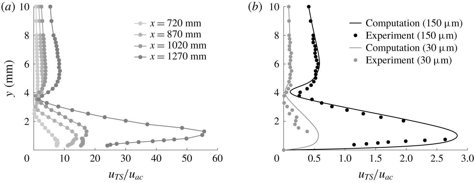
Figure 4. (a) Tollmien–Schlichting profiles at different streamwise stations for  $h=600~\unicode[STIX]{x03BC}\text{m}$ (
 $h/\unicode[STIX]{x1D6FF}_{B}^{\ast }=0.504$). (b) Comparison of computed and measured T–S amplitudes for (grey)
  $30~\unicode[STIX]{x03BC}\text{m}$ and (black)
  $150~\unicode[STIX]{x03BC}\text{m}$ (
 $h/\unicode[STIX]{x1D6FF}_{B}^{\ast }=0.025$ and 0.126, respectively) at
  $x=1320~\text{mm}$.
The T–S disturbance amplitude can be obtained by extracting the maxima in figure 4(b) for all roughness heights and customarily normalising it by the acoustic wave amplitude (Saric Reference Saric1994; Raposo et al. Reference Raposo, Mughal and Ashworth2018). These results are shown in figure 5, where the roughness height is normalised with the local boundary layer displacement thickness (at the location of the measurements). The left-hand side presents the T–S response to protuberances, whilst the right-hand side shows the equivalent for cavities. Both positive and negative displacements show the existence of a clear linear regime – within reasonable experimental uncertainty – where the T–S amplitude varies linearly with roughness height. The experimental data fit the linear trend remarkably well in the case of positive roughness heights in figure 5(a), whilst the scatter is higher for the negative heights in figure 5(b). It was found that for cavities  $|h|<200~\unicode[STIX]{x03BC}\text{m}$ (
 $|h|<16.8\,\%\unicode[STIX]{x1D6FF}_{B}^{\ast }$) the numerics tended to underestimate the experimentally measured amplitudes. The different behaviour for small protuberances and cavities contradicts results obtained from linearised boundary conditions and needs to be further explored. However, considering the experimental uncertainty affecting the measurements, the comparison with computed amplitudes is deemed satisfactory for small values of positive and negative displacements. This demonstrates the successful outcome of the improved data extraction technique applied in this work. Results also show that the departure from the linear regime takes place for absolute roughnesses height larger than
  $150~\unicode[STIX]{x03BC}\text{m}$ (
 $|h|>12.6\,\%\unicode[STIX]{x1D6FF}_{B}^{\ast }$). This is in line with previous work (Saric Reference Saric1994) at similar Reynolds numbers (
 $Re_{x}\approx 2.7\times 10^{6}$). It must be stressed, however, that this comparison must be taken with caution as the previous data are characterised by overall different external conditions: non-dimensional frequency (
 $F\,\approx \,50$), measurement locations (
 $x=1.83~\text{m}$), relative roughness height
  $1\,\%<h/\unicode[STIX]{x1D6FF}_{B}<8\,\%$, sound field
  $\text{SPL}>90~\text{dB}$, and
  $Tu=0.016\,\%U_{\infty }$. However, these data represent one of the most comprehensive experimental datasets on this topic, hence justifying the qualitative comparison discussed here. The breakdown of the linear relationship between roughness height and disturbance amplitude, however, seems to be geometry dependent as, in the case of depressions, the amplitude shows a stronger deviation from the numerical results at
  $|h|=200~\unicode[STIX]{x03BC}\text{m}$ (
 $|h|=16.8\,\%\unicode[STIX]{x1D6FF}_{B}^{\ast }$, the first empty marker). This complements previous findings that only considered positive roughnesses (Saric Reference Saric1994; Raposo et al. Reference Raposo, Mughal and Ashworth2018). Also of note is the fact that the nonlinear response is greater for the positive roughness heights than it is for the corresponding negative cases for
  $|h|\gg 200~\unicode[STIX]{x03BC}\text{m}$ (
 $|h|/\unicode[STIX]{x1D6FF}_{B}^{\ast }\gg 0.168$); the non-dimensional T–S amplitude for
  $|h|=50.4\,\%\unicode[STIX]{x1D6FF}_{B}^{\ast }$ is shown to be 56, whilst it is only 25 for its negative counterpart.

Figure 5. Effect of (a) positive, and (b) negative roughness heights (i.e. protuberances and cavities) on the excitation of T–S instability. Conditions:  $L=570~\text{mm}$,
  $F\approx 25.85$, whilst
  $x=1320/1270~\text{mm}$ for roughness heights below/above
  $|h|=200~\unicode[STIX]{x03BC}\text{m}$ (
 $|h|=16.8\,\%\unicode[STIX]{x1D6FF}_{B}^{\ast }$).
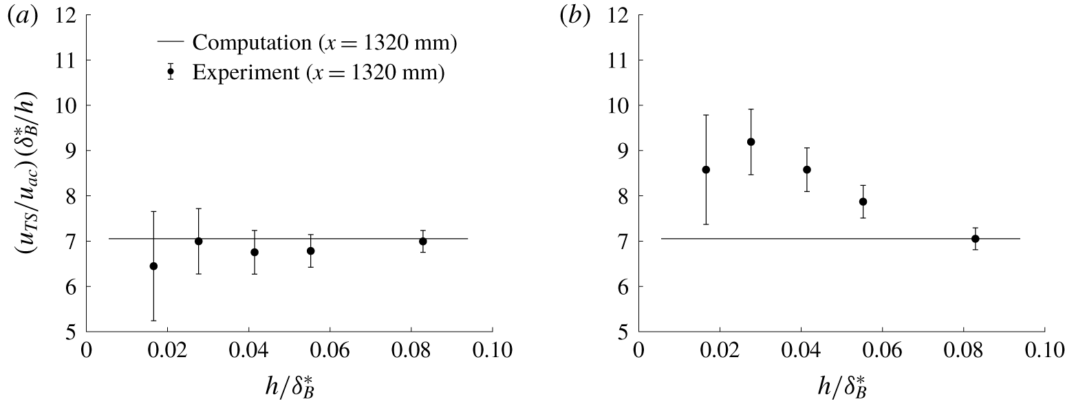
Figure 6. Effect of (a) positive, and (b) negative roughness heights on the excitation of T–S instability. Error bars are the uncertainty on T–S amplitudes.
Additionally, the flow at streamwise station  $x=1270~\text{mm}$ was found to be fully turbulent for
  $h=750~\unicode[STIX]{x03BC}\text{m}$ (
 $h=63.0\,\%\unicode[STIX]{x1D6FF}_{B}^{\ast }$) – and hence omitted, whilst still laminar at matched negative height. It has been shown that even for
  $Re_{h}\approx 0.1$ a separation bubble exists aft of a rectangular two-dimensional roughness element, with its reattachment length depending on the height of the roughness itself. This separation can form a free shear layer exhibiting its own instability, which can alter the local receptivity process (Saric & Krutckoff Reference Saric and Krutckoff1990; Crouch Reference Crouch1992). Similarly, a recirculating bubble is expected to form within the cavity for significant heights, which can reduce the effective cavity depth seen by the flow. It is perhaps not counterintuitive to imagine these two geometries behaving differently, with repercussions on the mean flow, and, hence leading to the breakdown of the assumptions underpinning linear theory. Next, we further explore the linear range presented in figure 5(a) by introducing an alternative normalisation which accounts for the step height, so that the linear regime becomes a constant. Here, we employ the disturbance amplitude in the outer lobe as this is more reliable (see the Appendix). This new normalisation is presented in figure 6, and it intended to enhance any discrepancies with the predicted linear behaviour. This confirms the presence of a clear linear regime for the positive heights, whilst the latter is less identifiable for their negative counterparts, as already highlighted in figure 5. This deserves further exploration; however, given the poor signal-to-noise ratio and high experimental uncertainty at these small roughness heights, caution must be applied when concluding on linear versus nonlinear behaviour. These findings need to be further investigated through more detailed near-field measurements and would benefit from complementary DNS. This behaviour was never discussed before due to the limitation in previously adopted techniques that limited the exploration to positive roughness heights. To conclude, the T–S disturbance amplitudes presented herein compare remarkably well with the numerical approach described in Raposo et al. (Reference Raposo, Mughal and Ashworth2018), and are also qualitatively consistent with previous work from Saric (Reference Saric1994), where, despite the different inflow conditions, a linear response between the disturbance amplitude and the height of the roughness was found to extend to protuberances approximately up to
  $150~\unicode[STIX]{x03BC}\text{m}$ high. Additionally, it was discussed in Raposo et al. (Reference Raposo, Mughal and Ashworth2018) how their methodology was found to be in agreement with quasi-parallel theory by Crouch (Reference Crouch1992) and Choudhari & Streett (Reference Choudhari and Streett1992); therefore, the current experimental results are, more broadly, strengthened and validated by previous numerical work on the topic. These findings highlight the potential of the retractable roughness technique used in this work.
4 Conclusions
Wind tunnel experiments on the receptivity of two-dimensional boundary layers dominated by T–S instability to acoustic disturbances coupled with two-dimensional roughness were performed in a low-turbulence wind tunnel in a zero-pressure-gradient boundary layer. A SL was produced by means of a free-stream acoustic wave generated by a loudspeaker. An improved experimental technique has been presented to separate the amplitudes of the T–S component from that of the SL. This technique is based on a vanishing roughness coordinated by a computer-controlled linear actuator during the data acquisition. Thanks to this set-up, both positive and negative roughnesses (protuberances and cavities, respectively) of  $30~\unicode[STIX]{x03BC}\text{m}<|h|<750~\unicode[STIX]{x03BC}\text{m}$ (
 $0.025<|h|/\unicode[STIX]{x1D6FF}_{B}^{\ast }<0.630$) were considered; cavities had not been explored before. Results show that for both positive and negative roughness heights, clear linear and nonlinear behaviours are identifiable. The onset of the nonlinear behaviour (based on T–S disturbance amplitude) is shown to be at approximately
  $\pm 150~\unicode[STIX]{x03BC}\text{m}$ (
 $|h|/\unicode[STIX]{x1D6FF}_{B}^{\ast }\approx 0.126$) in qualitative agreement with previous evidence. Furthermore, the receptivity to small negative heights (cavities with
  $|h|/\unicode[STIX]{x1D6FF}_{B}^{\ast }<0.168$) seems to be greater than that of comparable protuberances. This needs to be explored further. Additionally, there is some indication that nonlinear effects can appear for shallower depressions; however, these are milder than in the case of positive roughness for more substantial heights, say
  $|h|>400~\unicode[STIX]{x03BC}\text{m}$ (
 $|h|/\unicode[STIX]{x1D6FF}_{B}^{\ast }>0.336$). This is possibly due to the flow physics within the cavity, which requires further investigation. Finally, the T–S disturbance amplitudes for positive heights were found to be in remarkable agreement with the computations based on Raposo et al. (Reference Raposo, Mughal and Ashworth2018), and the earlier work of Crouch (Reference Crouch1992) and Choudhari & Streett (Reference Choudhari and Streett1992), which predicted a linear disturbance response to small-height perturbations. This evidence highlights the validity of the technique presented herein to successfully separate the SL from the T–S contribution.
Acknowledgements
We would like to acknowledge the financial support of the EPSRC (EP/L024888/1) and Airbus Central R&T. We are indebted to the authors of Raposo et al. (Reference Raposo, Mughal and Ashworth2018), particularly H. Raposo, for their support in designing the tests, and for providing numerical results for comparison. We also want to acknowledge Dr E. van Bokhorst, who provided us with data for some of the further comparisons contained in the Appendix.
Declaration of interests
The authors report no conflict of interest.
Appendix. Method validation and sensitivity tests
This appendix expands on the methodology validation and presents sensitivity tests of the measured disturbance amplitude to different quantities of interest. Figure 7(a) compares the evolution of the T–S mode shapes between the numerics and the measurements. This comparison is presented for the  $h=150~\unicode[STIX]{x03BC}\text{m}$ case (
 $h/\unicode[STIX]{x1D6FF}_{B}^{\ast }=0.126$) across the measurement stations (
 $870~\text{mm}<x<1320~\text{mm}$). A remarkable agreement is shown for the magnitude, and shape, of the outer lobe of the disturbance at
  $x=1320~\text{mm}$ where the signal-to-noise ratio is maximised. It is worth stressing that using the disturbance outer lobe can provide a more resilient methodology; however, we have here employed the inner lobe maximum to quantify the disturbance strength in accordance with previous work. Computed and measured change in N-factor between the measurement stations were found to be within 2 %. Figure 7(b) is a replica of figure 5(a); however, it includes a subset of data points to explore the sensitivity of the boundary layer to the level of acoustic forcing, and to assess the three-dimensionality of the T–S disturbance. It is shown from off-centre measurements (filled square symbol), that the disturbance can be considered largely two-dimensional as the slight amplitude difference across the spanwise stations is within experimental uncertainty. Furthermore, as discussed in § 2.2, a SPL of
  $80~\text{dB}$ was chosen to guarantee a linear response of the boundary layer to the acoustic forcing. Sensitivity tests on a reduced number of step heights were also carried out to explore the dependence of the onset of the nonlinear response of the boundary layer to the acoustic field. The measurements (empty square symbols) confirm that the upper boundary of the linear response is found to be dependent on the level of the acoustic oscillation, confirming previous literature (Saric Reference Saric1994). It is observed that for
  $\text{SPL}=70~\text{dB}$, the disturbance response remains close to the linear trend up to higher roughness heights (
 $h=400~\unicode[STIX]{x03BC}\text{m}$ or
  $h/\unicode[STIX]{x1D6FF}_{B}^{\ast }>0.336$). Finally, preliminary tests were carried out by Dr van Bokhorst, employing both a static subtraction technique (i.e. a plate with a machined slot cut into it) and the burst-sound technique. These tests were carried out on a
  $750~\unicode[STIX]{x03BC}\text{m}$ deep cavity roughness and at a marginally different Reynolds number; however, the disturbance amplitudes were found to be within 2.5 % and 20 %, respectively, of those of the current measurements.
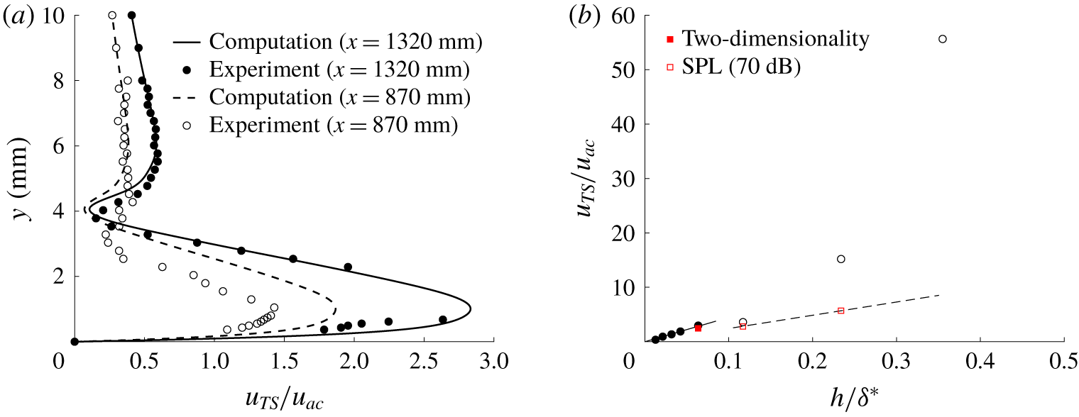
Figure 7. (a) T–S mode shapes at different streamwise stations for  $h=150~\unicode[STIX]{x03BC}\text{m}$ (
 $h/\unicode[STIX]{x1D6FF}_{B}^{\ast }=0.126$). (b) Sensitivity tests to acoustic disturbance levels, and two-dimensionality of the disturbance. See legend in figure 5 for other symbols.


 Open access