


NOMENCLATURE
- a
-
speed of sound
- BPR
-
by-pass ratio
- D
-
nozzle exit or jet diameter
- EPN
-
effective perceived noise
- f
-
frequency
- FWH
-
Ffowcs Williams–Hawkings
- H 12
-
boundary-layer shape factor (
 $\delta^{\ast\!}/\theta$
)
$\delta^{\ast\!}/\theta$
) - IR
-
infra-red
- k
-
turbulence kinetic energy
- L
-
axial length
- LES
-
large-eddy simulation
- M
-
Mach number
- NPR
-
nozzle pressure ratio (p t,j /p amb)
- NTR
-
nozzle temperature ratio (T t,j /T s,amb)
- OASPL
-
overall sound pressure level
- p
-
pressure
- PSD
-
power spectral density
- r
-
radial distance, shear-layer velocity ratio
- r ij,kl
-
dimensional two-point two-time correlation
- R ij,kl
-
non-dimensional two-point two-time correlation
- RANS
-
Reynolds-averaged Navier–Stokes
- Re
-
Reynolds number
- s
-
shear-layer density ratio
- St
-
Strouhal number
- T
-
temperature
- t
-
jet/ambient static temperature ratio (T s,j /T s,a )
- U, V, W
-
velocity components
- u, v, w
-
rms turbulence fluctuating velocity components
- x, y, z
-
spatial co-ordinates

GREEK SYMBOLS
-
${\delta}^{\ast}$
-
displacement thickness
-
${\delta}$
’
-
shear-layer growth rate
- ɛ
-
turbulence energy dissipation rate
- η
-
spatial separation
-
${\theta}$
-
momentum thickness, azimuthal angle, polar angle
-
${\mu}$
-
viscosity
- ρ
-
density
- τ
-
temporal separation
-
${\phi}$
-
observer polar angle
-
${\omega}$
-
vorticity


Subscripts
-
$a,\,\textrm{amb}$
-
atmospheric ambient property
- bp
-
by-pass property
- c
-
convective
- cl
-
centreline property
- core
-
jet core property
- fs
-
flight stream property
-
$i,\,j,\,k,\,l$
-
tensor indices
- j
-
jet/nozzle exit property
- on
-
onset flow
- PC
-
potential core
- rms
-
root mean square
- s
-
static property
- t
-
total property
- 1,2
-
fast and slow streams in planar shear layer


1.0 Introduction
Examples abound of turbulent jet flows in both the natural and engineering world. Jet flows occur in all engineering disciplines: water outfalls, cooling tower plumes and ventilation flows in civil/building engineering, mixing and reaction vessels in chemical engineering, cooling of electronic components, and mixing, heating and cooling technologies in mechanical engineering. The present focus is on aerospace (space rocketry and missiles excluded) where jets generate propulsive thrust for flight in both civil and military aircraft.
In civil aerospace, designers require an understanding of jet plume development from engine exhaust nozzles and methods to manipulate this to meet legislation governing aircraft noise. The International Civil Aviation Organization (ICAO) via its Committee on Aviation Environmental Protection (CAEP) sets international environmental standards for civil aviation. The CAEP has published a series of regulations for subsonic aircraft noise: originally Chapter 3 in 1977, and mandating further reductions over time relative to Chapter 3 in 2006 (–10dB) and 2017 (–17dB). Engine manufacturers have continually designed to achieve reduced noise (Fig. 1). In 2000, the European Union (EU) set aircraft/engine manufacturers performance improvement targets for CO2, pollutant emissions and noise reduction: Vison 2020 (2) and Flightpath 2050 (2050 target shown by open circle in Fig. 2) (3). Figure 2 illustrates the progress made by Rolls-Royce, whose engines are now 20–30dB quieter than early turbojets; noise level is reducing by
 $\sim$
0.5dB/year but further and faster progress is required.
$\sim$
0.5dB/year but further and faster progress is required.
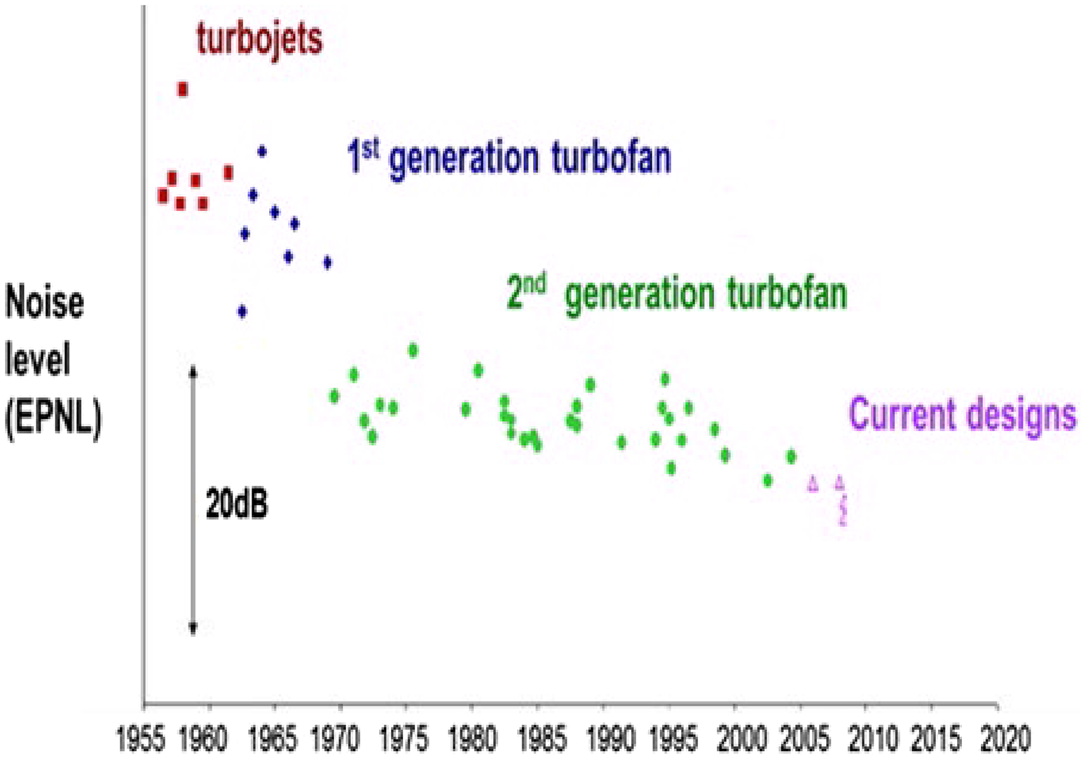
Figure 1. Aircraft noise reduction over time, effective perceived noise level from Ref. Reference Astley, Agarwal, Joseph, Self, Smith, Sugimoto and Tester1.
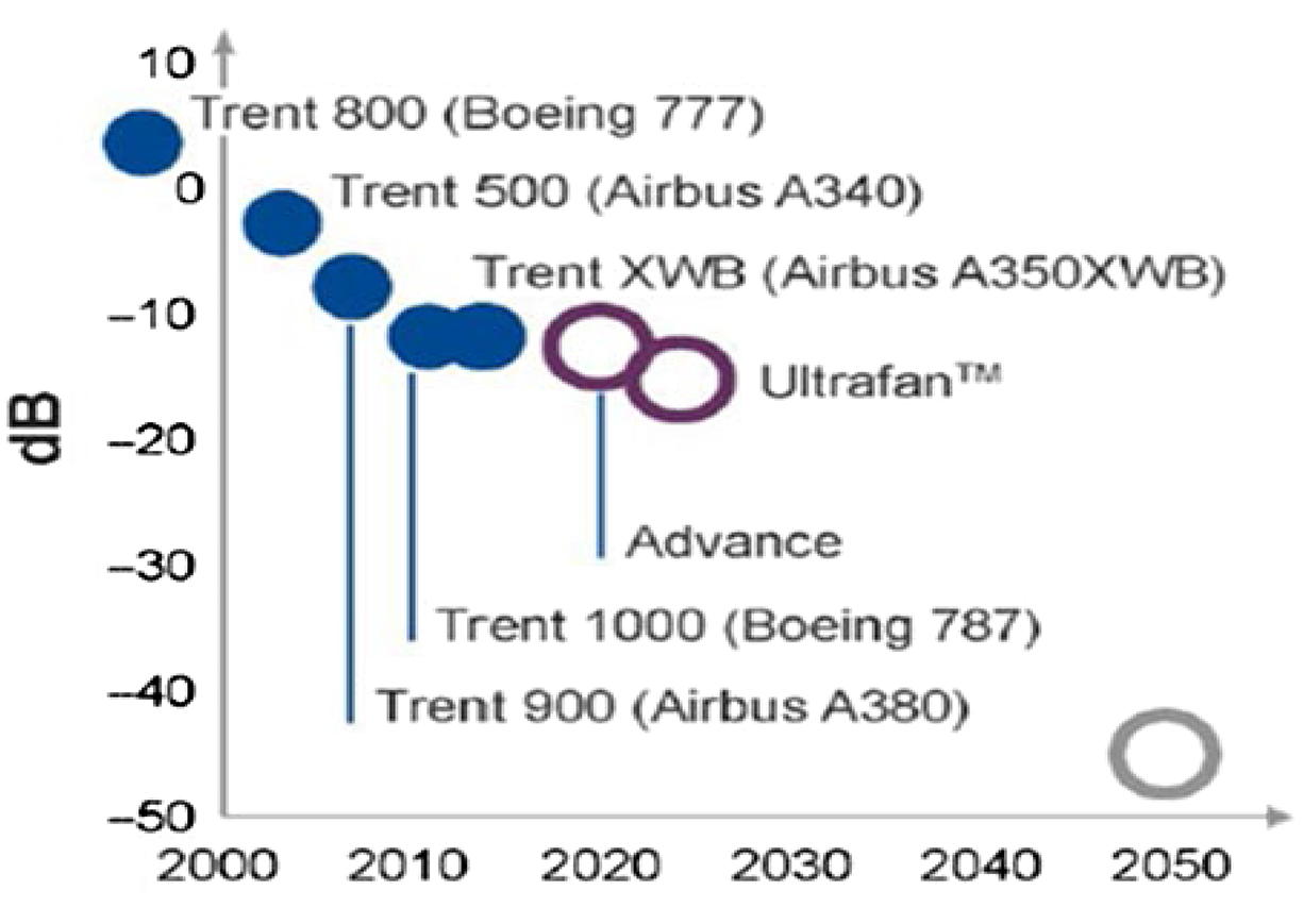
Figure 2. Flightpath 2050-driven noise level reductions in Rolls-Royce engines.
Several engine noise sources contribute to aircraft noise; see Fig. 3 for typical conditions at departure. In modern engines with high by-pass ratio, whilst combustor and compressor/turbine turbomachinery make a contribution, fan and jet noise are dominant components at take-off; the ‘bubbles’ in Fig. 4 indicate the regions/directions where each component is influential. Reducing jet noise is thus the primary reason civil aeroengine designers require accurate knowledge of propulsion jet aerodynamics/aeroacoustics.
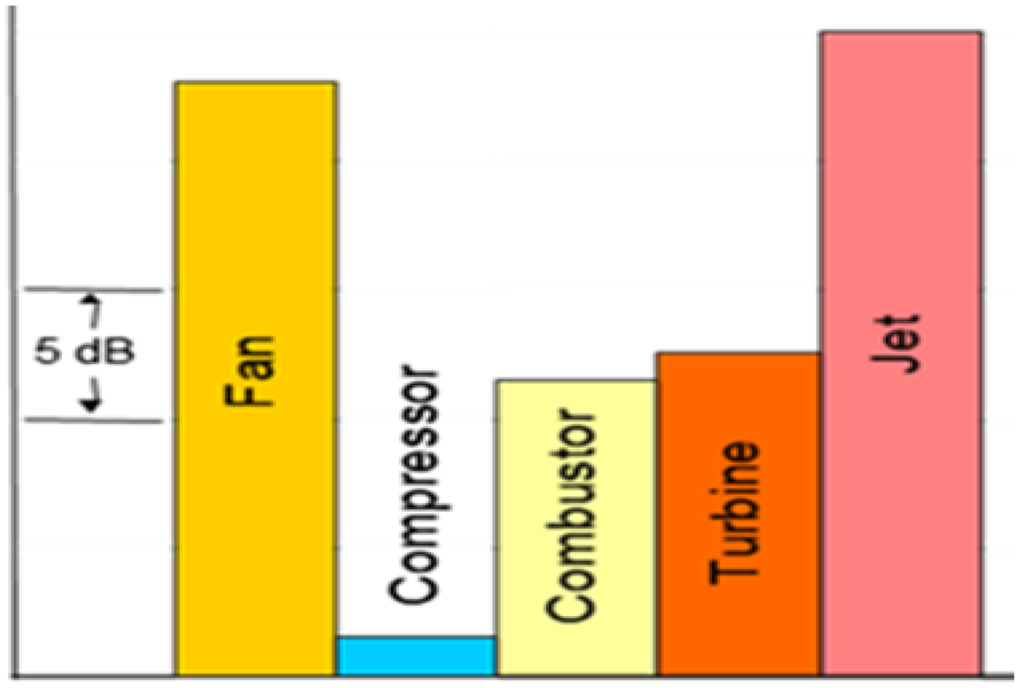
Figure 3. Noise source contributions for aircraft departure conditions from Ref. Reference Astley, Agarwal, Joseph, Self, Smith, Sugimoto and Tester1.
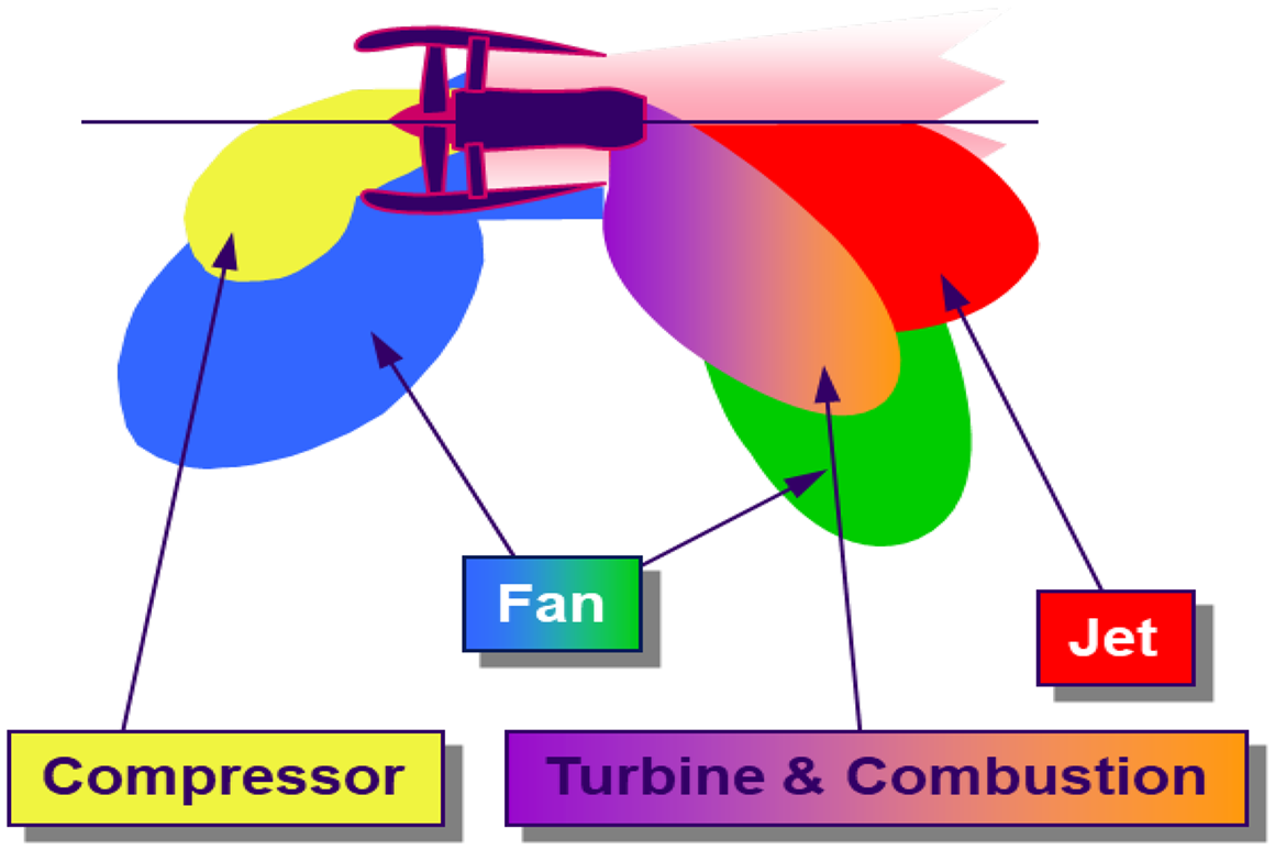
Figure 4. Noise source distribution for a modern engine from Ref. Reference Astley, Agarwal, Joseph, Self, Smith, Sugimoto and Tester1.
In terms of the velocity at the exhaust nozzle exit (U
j
), the move from turbojet to turbofan, and the growth in by-pass ratio (BPR = by-pass flow/core flow) and fan diameter has brought about a large reduction in U
j
. Theoretical analysis of jet aeroacoustics by Lighthill (Reference Lighthill4) indicated that jet noise is a strong function of jet velocity (
 $\sim$
U
j
8); lowering U
j
is thus an important approach to decrease the jet noise contribution (Fig. 1). That work also revealed that the noise source was driven by turbulence created in the jet–ambient mixing process. It also indicated that high-order turbulent correlations are involved – fourth-order spatio-temporal correlations – making CFD prediction of jet noise challenging. However, recent progress in advanced methods based on LES CFD is promising, although as described below, inadequacies still exist and computational cost is high.
$\sim$
U
j
8); lowering U
j
is thus an important approach to decrease the jet noise contribution (Fig. 1). That work also revealed that the noise source was driven by turbulence created in the jet–ambient mixing process. It also indicated that high-order turbulent correlations are involved – fourth-order spatio-temporal correlations – making CFD prediction of jet noise challenging. However, recent progress in advanced methods based on LES CFD is promising, although as described below, inadequacies still exist and computational cost is high.
As the BPR increases (>10 is typical), the slow by-pass and faster core flow can be mixed to lower the mass-average U J . This leads to the introduction of so-called forced mixers with various geometries but typically comprising multiple azimuthally distributed variously shaped lobes (plain, scarfed, scalloped, etc.), as illustrated in Fig. 5. Whilst mixing by-pass and core flows is beneficial to jet noise, mixing device total pressure losses and extra weight/increased cowl length (drag penalty) mean that a trade-off is required depending on aircraft design mission length to determine whether such devices are affordable. In recent years, more subtle devices have become popular – serrations or chevrons cut into the by-pass nozzle (and possibly also the core), as shown in Fig. 6. Detailed mechanisms behind this technology are described below.
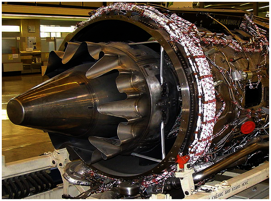
Figure 5. Lobed mixer (by-pass nozzle wall removed) BR715 engine, Boeing 717 aircraft.
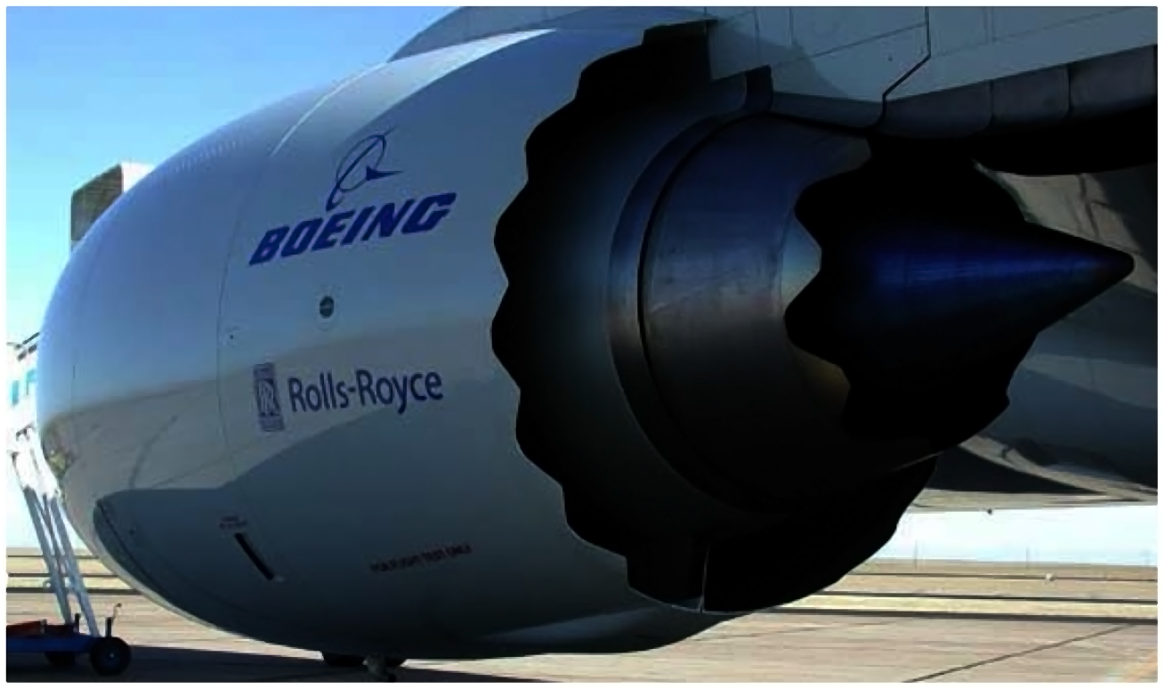
Figure 6. Serrated nozzles on both by-pass and core ducts on Boeing 787 aircraft.
A further civil aerospace mixed aerodynamic–aeroacoustic application involving the jet plume is jet installation noise (Fig. 7). This illustrates an increasingly more common scenario as turbofan diameter increases and (to avoid longer undercarriage) engines are installed closer to the wing. The left-hand image indicates the extra noise phenomena introduced by jet–wing interactions. The first occurs when jet/ambient shear-layer noise is reflected towards the ground by the wing under-surface. The second results from jet–surface aerodynamic interactions – the flow field in the wing/flap vicinity is modified by the jet flow, thus altering the generation of trailing-edge noise. If high-lift devices on the wing are fully deployed, the spreading jet edge flow may even impinge on the flap. The right-hand images in Fig. 7 are taken from an LES CFD study (Reference Angelino, Moratilla-Vega, Howlett, Xia and Page5) described below and indicate how the flow is influenced by different flap deflections and engine–wing separations.
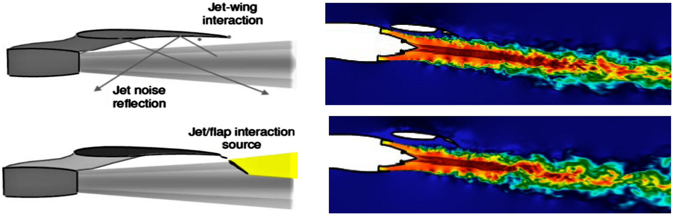
Figure 7. Jet wing interaction noise – from Ref. Reference Astley, Agarwal, Joseph, Self, Smith, Sugimoto and Tester1 (left) and Reference Angelino, Moratilla-Vega, Howlett, Xia and Page5 (right).
In military aircraft, jet velocities can be supersonic and improperly expanded, causing ‘shock diamonds’ in the jet plume (Fig. 8). Depending on the Nozzle Pressure Ratio (NPR = nozzle inlet total pressure/ambient static pressure), an additional acoustic effect – screech – can also occur. This is self-sustaining, high-intensity, tonal noise caused by an aeroacoustic resonance loop within the flow. If sufficiently intense and at a frequency close to structural resonances, damage can result. It is clearly essential for designers to understand the NPRs at which this occurs and be able to predict the intensity of pressure oscillations. Figure 8 also shows that, in this application (with afterburners), the jet plume is significantly hotter than in civil applications. A second design motivation is thus to enhance jet plume mixing to reduce the aircraft’s Infra-Red (IR) signature and improve low observability. Nozzle cross-sections that enhance mixing and technologies to increase mixing (tabs, fluid injection and plasma actuators) are also of design interest. Letterbox rectangular nozzles, aligned to match the aircraft shape and discharging over an ‘aft-deck’, are of potential interest, (Fig. 9), requiring effects of shape, entrainment restriction, etc. to be accurately captured.
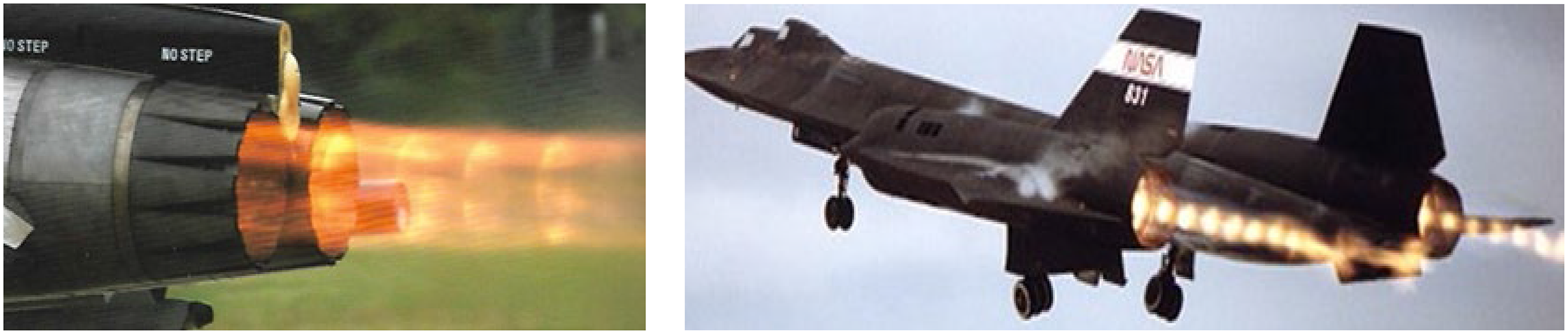
Figure 8. Examples of shock-containing hot jet plumes.
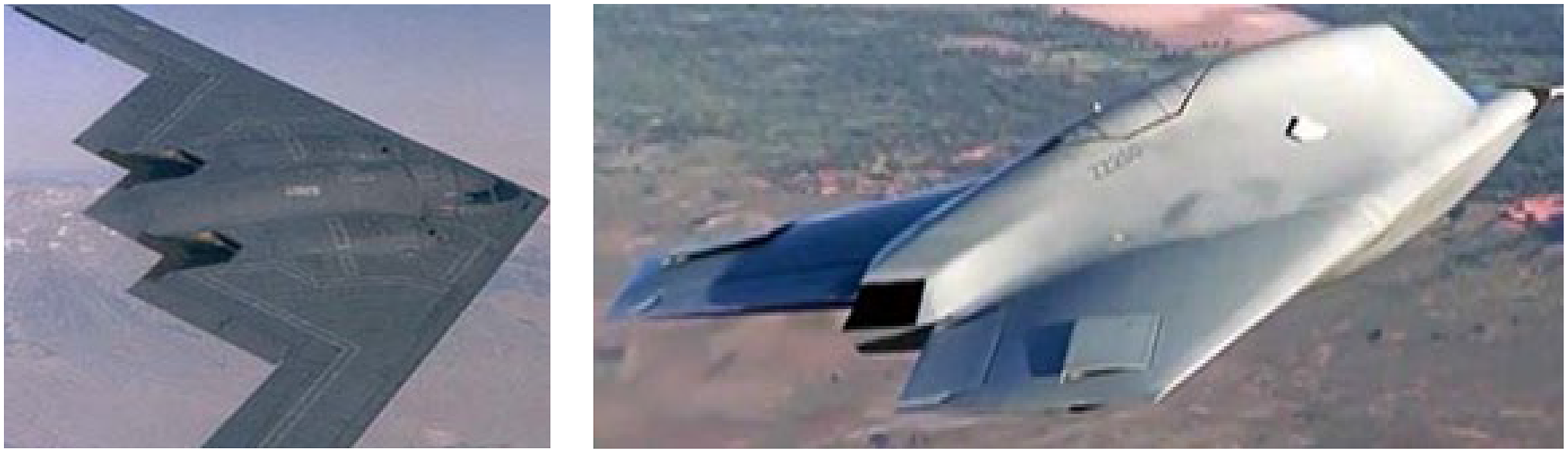
Figure 9. Non-axisymmetric nozzle cross-section with aft-deck: B2 (left) and BAeS-Taranis (right).
Finally, for VSTOL aircraft such as the Harrier or F-35, the influence of the propulsion jet plume(s) on the overall aircraft aerodynamics is particularly complex. This is the case for manoeuvres such as the transition from forward flight into vertical descent and the vertical landing itself, where phenomena such as lift jet splay angle, hot-gas ingestion, fountain upwash and ground vortex flows, illustrated in Fig. 10, must be carefully assessed.
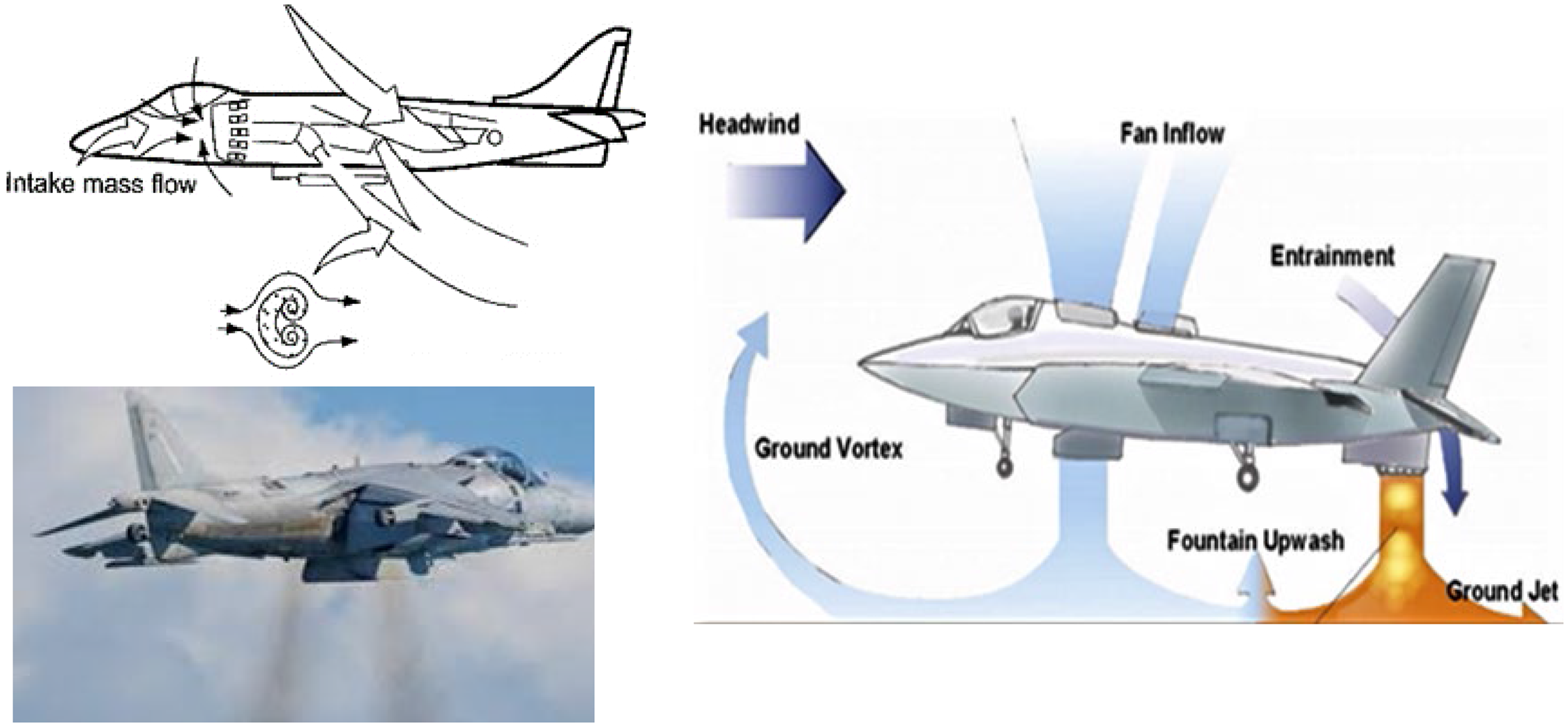
Figure 10. V/STOL aircraft aerodynamics for BAe Harrier (left) and F35 (right).
The above brief review reveals and illustrates the several challenges faced by aerospace engineers when considering aspects of engine or airframe design which are influenced by propulsion jet plume development. The rest of this paper is organised as follows: firstly, in Section 2, fundamental aerodynamic and aeroacoustic processes which influence jets are summarised; secondly, in Sections 3 and 4, the progress made over the last decade or two in developing LES-based predictive approaches for the various civil and military applications described is outlined. Particular emphasis is placed on the extent to which these approaches have been validated against carefully chosen measurements. Finally, Section 5 provides a summary, the conclusions and suggestions for further work.
2.0 Fundamental characteristics of jet flows
2.1 Aerodynamics aspects
Jet flow pattern
The basic fluid mechanics of a simple round jet in stagnant surroundings is sketched in Fig. 11. At the nozzle exit, two regions form: a potential core (of length X PC) within which velocity remains at U J , and an annular shear layer growing with x. For the Re j = ρ j U j D j /μ j values of practical configurations (on the order of 106–107), the nozzle exit boundary layer will be turbulent and turbulent mixing dominates shear-layer growth; these exit conditions influence the transformation from the initial shear layer to a fully formed, round jet as well as X PC. The region of interest here is the jet near field (x/D j < 20); it is thus important that the flow/turbulence conditions at the exit be considered in both CFD predictions and laboratory experiments if these are to be representative (although, until recently, this was rarely the case, as discussed below). Further downstream (x/D j > 30) a self-similarity region is found (Reference Pope6), with the value of the asymptotic growth rate playing an important role in calibrating constants in RANS turbulence models.
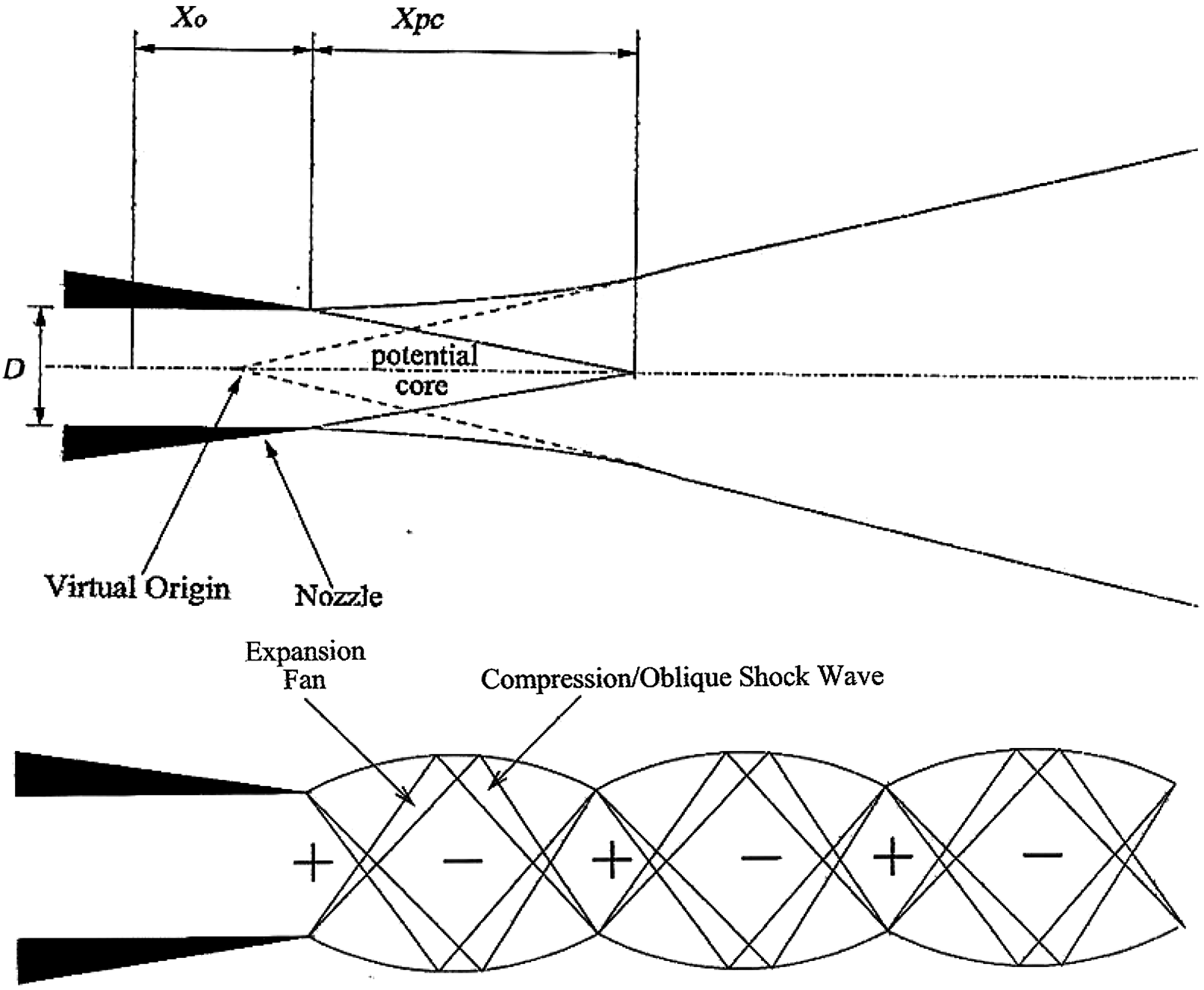
Figure 11. Jet flow development from convergent round nozzle: subsonic and supersonic.
This description is relevant to low-speed jets (Mach no. M j < 0.5), whereas aerospace applications involve transonic and supersonic M j . At nozzle NPRs >1.89 (for air), shock-containing under-expanded (convergent nozzle) or under- and over-expanded jets (con-di nozzle) are possible. Expansion and oblique shock waves appear in the jet near-field; see Fig. 11 for a moderately under-expanded convergent nozzle. The colour Schlieren photographs in Fig. 12 are typical of high-speed aerospace applications; the upper two images correspond to a convergent round nozzle producing a weakly under-expanded jet (NPR = 2.3) and a moderately under-expanded jet with stronger shock waves (NPR = 4.0), whereas the lower two images show con-di nozzle under- and over-expanded flows (nozzle geometry design NPR = 3.5).
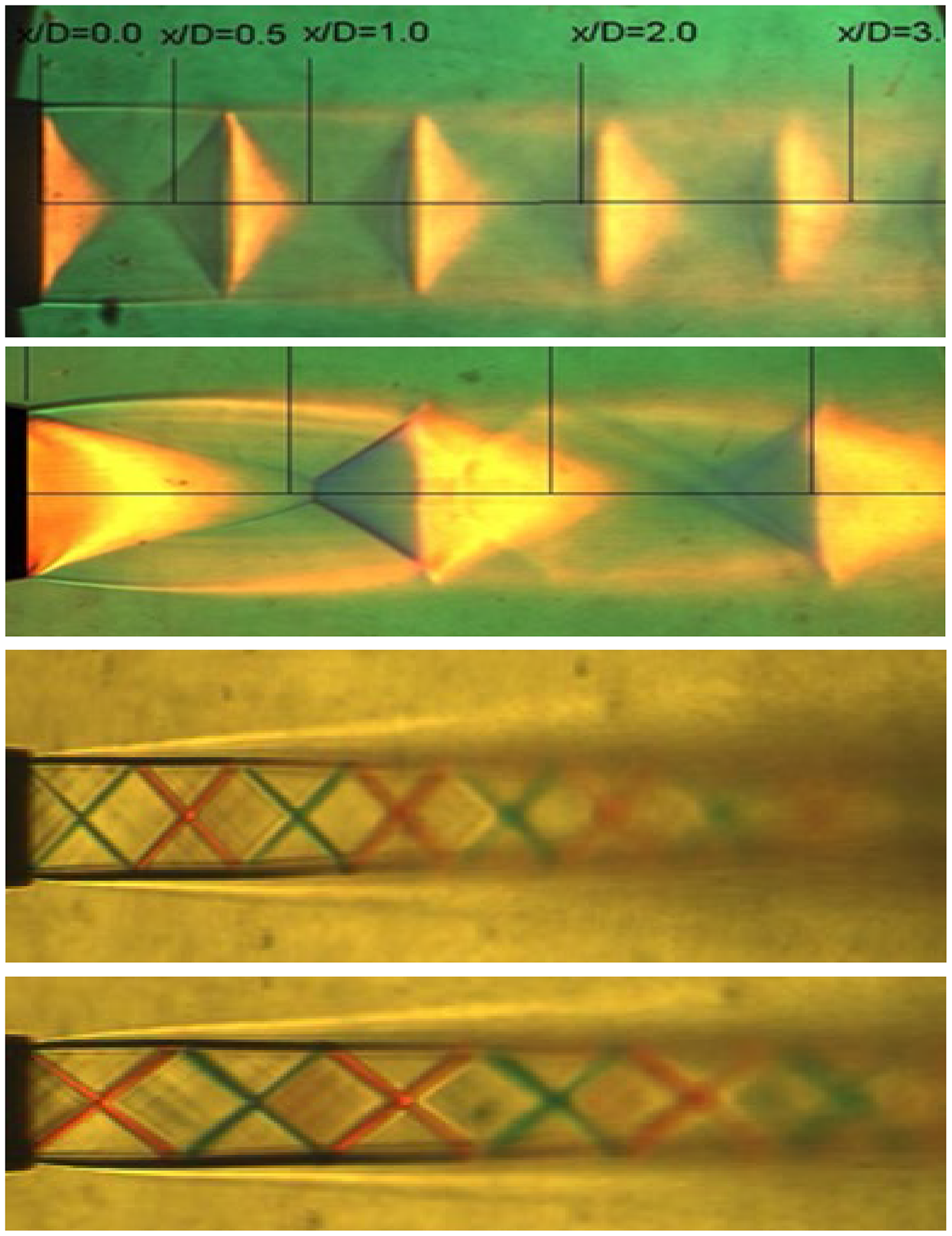
Figure 12. Schlieren images: under-expanded, NPR 2.3, 4.0 (top) and con-di, NPR = 3.3, 3.8 (bottom).
Jet Reynolds number effects/nozzle exit conditions
Potential core length is an important parameter for military applications since this is the region of highest temperature and IR signature; it is also the parameter most likely to be affected by nozzle exit conditions. Adequate consideration of these in laboratory studies intended to be relevant to propulsion nozzles has only recently been realised. Literature reviewed in Trumper et al. (Reference Trumper, Behrouzi and McGuirk7) indicates that early experimental studies considered too low Re
j
or exit profiles far removed from operating conditions relevant to aero-propulsion. Even early LES studies commonly reduced the computed Re
j
by a factor of
 $\sim$
10 to ease the mesh resolution requirement. To match operational conditions, minimum laboratory test values for Re
j
are important. Birch (Reference Birch8) concluded that “laminar viscosity has little influence on jet mixing, Re
j
enters the problem only because the thickness of the initial wall boundary layer depends on Re
j
….it is the initial boundary layer that is the controlling factor not Re
j
…”. Based on this, a minimum value of Re
j
= 4 × 10⁵ was recommended. Further complication is introduced by the acceleration within the nozzle, which can lead to boundary layer relaminarisation (Reference Narasimha and Sreenivasan9). Probably the first set of measurements to pay attention to this issue was reported by Bridges and Wernet (Reference Bridges and Wernet10), who used a hot-wire probe to characterise the nozzle exit boundary layer and clearly illustrated the problem of high acceleration and too low Re
j
. Two nozzle convergence geometries were used: the first produced a boundary layer shape factor of H
12
$\sim$
10 to ease the mesh resolution requirement. To match operational conditions, minimum laboratory test values for Re
j
are important. Birch (Reference Birch8) concluded that “laminar viscosity has little influence on jet mixing, Re
j
enters the problem only because the thickness of the initial wall boundary layer depends on Re
j
….it is the initial boundary layer that is the controlling factor not Re
j
…”. Based on this, a minimum value of Re
j
= 4 × 10⁵ was recommended. Further complication is introduced by the acceleration within the nozzle, which can lead to boundary layer relaminarisation (Reference Narasimha and Sreenivasan9). Probably the first set of measurements to pay attention to this issue was reported by Bridges and Wernet (Reference Bridges and Wernet10), who used a hot-wire probe to characterise the nozzle exit boundary layer and clearly illustrated the problem of high acceleration and too low Re
j
. Two nozzle convergence geometries were used: the first produced a boundary layer shape factor of H
12
 $\sim$
2.4 (clearly laminar), while the second lowered this (2.0) but still resulted in a transitional boundary layer. To avoid these problems, Trumper et al. (Reference Trumper, Behrouzi and McGuirk7) combined a higher bulk Re
j
(
$\sim$
2.4 (clearly laminar), while the second lowered this (2.0) but still resulted in a transitional boundary layer. To avoid these problems, Trumper et al. (Reference Trumper, Behrouzi and McGuirk7) combined a higher bulk Re
j
(
 $\sim$
106) with a small parallel-wall extension at the nozzle exit to allow boundary-layer recovery, whilst maintaining an acceleration broadly similar to the BAE Systems Hawk aircraft nozzle. The success of this strategy is indicated in Fig. 13 and Table 1. The former shows that the exit velocity profile with extension (LU60(P)) is clearly more turbulent. Table 1 illustrates that the short exit extension produces a fully turbulent shape factor (1.22) as opposed to the laminar-like nature of the datum nozzle with no extension (2.02). The exit momentum thickness increased by a factor of
$\sim$
106) with a small parallel-wall extension at the nozzle exit to allow boundary-layer recovery, whilst maintaining an acceleration broadly similar to the BAE Systems Hawk aircraft nozzle. The success of this strategy is indicated in Fig. 13 and Table 1. The former shows that the exit velocity profile with extension (LU60(P)) is clearly more turbulent. Table 1 illustrates that the short exit extension produces a fully turbulent shape factor (1.22) as opposed to the laminar-like nature of the datum nozzle with no extension (2.02). The exit momentum thickness increased by a factor of
 $\sim$
14, although the boundary layer was still substantially thinner (by a factor of
$\sim$
14, although the boundary layer was still substantially thinner (by a factor of
 $\sim$
6) than at the nozzle inlet.
$\sim$
6) than at the nozzle inlet.
Table 1. Momentum thickness and shape factor at nozzle inlet/exit from Ref. Reference Trumper, Behrouzi and McGuirk7
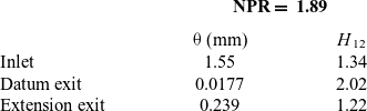
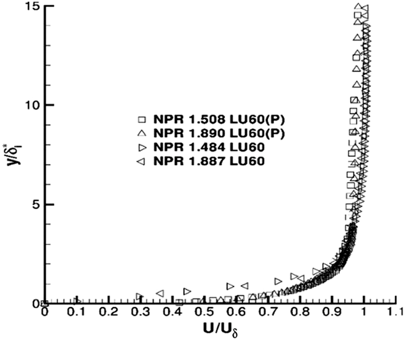
Figure 13. Nozzle exit axial velocity profiles from Ref. Reference Trumper, Behrouzi and McGuirk7. Datum nozzle (LU60) and with extension (LU60P).
The sensitivity of the developing jet shear layer to changed nozzle exit conditions is quantified in Fig. 14, which shows the measured mean axial velocity along the centreline (top) and the nozzle lipline (bottom with axial velocity on the left and axial rms on the right). Centreline and lipline velocities for the datum nozzle are lower than with an extension, only for a short distance on the centreline but larger differences were observed on the lipline up to x/D = 5. Lipline axial rms turbulence is
 $\sim$
7% larger without extension, but this difference disappears after
$\sim$
7% larger without extension, but this difference disappears after
 $\sim$
2D. These are relatively small changes, but they may contribute to differences in high-frequency noise generation since this is dominated by the early shear-layer region. Measuring velocity and turbulence conditions at the nozzle inlet and exit is useful in all measurements, but especially for CFD validation data.
$\sim$
2D. These are relatively small changes, but they may contribute to differences in high-frequency noise generation since this is dominated by the early shear-layer region. Measuring velocity and turbulence conditions at the nozzle inlet and exit is useful in all measurements, but especially for CFD validation data.
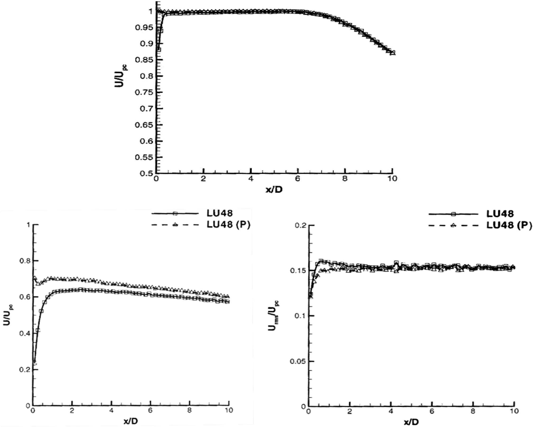
Figure 14. NPR = 1.89: centreline, axial velocity (top) and lipline axial velocity (bottom left) and axial rms (bottom right) from Ref. Reference Trumper, Behrouzi and McGuirk7.
Jet Mach number effects
An experimental study of planar shear layers between two high-speed streams by Papamoschou and Roshko (Reference Papamoschou and Roshko11) produced evidence that the layer thickness growth rate was reduced by compressibility (where the shear-layer thickness was defined via the vorticity thickness
 ${\delta _\omega } = ({U_1} - {U_2})/{(\partial U/\partial y)_{\max }}$
, where the velocities of the fast and slow streams are U
1 and U
2. The reduction was correlated well by the convective Mach number (M
c
), the Mach number in a frame of reference moving with the speed of shear layer instability waves or disturbances such as turbulent structures. If both streams are pressure matched and have the same ratio of specific heats, M
c
is defined by Equation (1), where a
1
and a
2
are the speed of sound in each stream. M
c
assumes the form of Equation (2) for the case of a jet in stagnant surroundings (U
1 = U
j
and U
2
= 0), where
${\delta _\omega } = ({U_1} - {U_2})/{(\partial U/\partial y)_{\max }}$
, where the velocities of the fast and slow streams are U
1 and U
2. The reduction was correlated well by the convective Mach number (M
c
), the Mach number in a frame of reference moving with the speed of shear layer instability waves or disturbances such as turbulent structures. If both streams are pressure matched and have the same ratio of specific heats, M
c
is defined by Equation (1), where a
1
and a
2
are the speed of sound in each stream. M
c
assumes the form of Equation (2) for the case of a jet in stagnant surroundings (U
1 = U
j
and U
2
= 0), where
 ${T_{s,j}},{T_a}$
are static temperatures in jet and ambient, respectively, with
${T_{s,j}},{T_a}$
are static temperatures in jet and ambient, respectively, with
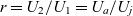
 $t = {T_{s,j}}/{T_a}$
. For isothermal jets, Mc = 0.5M
j
, although if the jet total temperature ratio is >1.0 (Nozzle Temperature Ratio (NTR) > 1), the factor will differ.
$t = {T_{s,j}}/{T_a}$
. For isothermal jets, Mc = 0.5M
j
, although if the jet total temperature ratio is >1.0 (Nozzle Temperature Ratio (NTR) > 1), the factor will differ.
 \begin{align}{M_C} = {{{U_1} - {U_2}} \over {{a_1} + {a_2}}}\end{align}
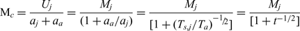 \begin{align}{{\textrm{M}}_c}={{{U_j}} \over {{a_j} + {a_a}}}={{{M_j}} \over {(1 + {a_a}/{a_j})}} = {{{M_j}} \over {[1 + {{({T_{s,j}}/{T_a})}^{{\raise0.5ex\hbox{$\scriptstyle { - 1}$}\kern-0.1em/\kern-0.15em\lower0.25ex\hbox{$\scriptstyle 2$}}}}]}} = {{{M_j}} \over {[1 + {t^{-1/2}}]}}\end{align}
This mechanism is very important for propulsive jets which have M
j
above 0.7 for civil and above 1.0 for military applications. The mechanism will increase the potential core length for high-Mach-number jets, and CFD must capture this for accurate IR signature estimation. Barone et al. (Reference Barone, Oberkampf and Blottner12) conducted a survey of several experimental investigations to confirm and expand on Ref. Reference Papamoschou and Roshko11. The black data points in Fig. 15 represent the data compiled, while the black dashed line shows the regression fit. The effect is significant, with the spreading rate halving for M
c
 $\sim$
0.8. Barone et al. (Reference Barone, Oberkampf and Blottner12) also compared their recommended curve against predictions from several RANS turbulence models, reaching the conclusion that all models captured the growth rate decrease but mainly based on incorrect assumptions. Recently, Feng and McGuirk (Reference Feng and McGuirk13), extending an earlier study by Lau et al. (Reference Lau, Morris and Fisher14), focused specifically on annular shear layers with greater relevance to the jet near field. This data, shown by the coloured points in Fig. 15, demonstrated that a similar effect as in planar shear layers was present, but with stronger suppression of growth rate with M
c
. Note also that, since the spreading rate is dependent on both M
c
and t (see below), the reduction in Fig. 15 is expressed relative to an incompressible shear layer with the same value of t (
$\sim$
0.8. Barone et al. (Reference Barone, Oberkampf and Blottner12) also compared their recommended curve against predictions from several RANS turbulence models, reaching the conclusion that all models captured the growth rate decrease but mainly based on incorrect assumptions. Recently, Feng and McGuirk (Reference Feng and McGuirk13), extending an earlier study by Lau et al. (Reference Lau, Morris and Fisher14), focused specifically on annular shear layers with greater relevance to the jet near field. This data, shown by the coloured points in Fig. 15, demonstrated that a similar effect as in planar shear layers was present, but with stronger suppression of growth rate with M
c
. Note also that, since the spreading rate is dependent on both M
c
and t (see below), the reduction in Fig. 15 is expressed relative to an incompressible shear layer with the same value of t (
 ${\delta _\omega }(0,t)$
). The temperature ratio t influences mixing even when compressibility is absent, as described in the next sub-section.
${\delta _\omega }(0,t)$
). The temperature ratio t influences mixing even when compressibility is absent, as described in the next sub-section.
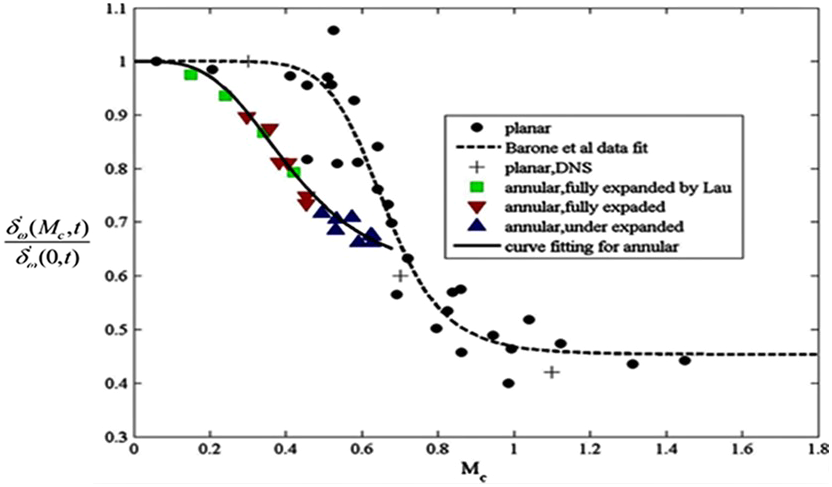
Figure 15. Compressibility-induced shear-layer spreading rate reduction from Refs Reference Barone, Oberkampf and Blottner12, Reference Feng and McGuirk13.
Jet temperature effects
Analogous to the study of compressibility in planar turbulent shear layers, Brown and Roshko (Reference Brown and Rosko15) carried out experiments to examine the effect of the density ratio across the shear layer
 $s = {\rho _2}/{\rho _1}$
(equivalent to
$s = {\rho _2}/{\rho _1}$
(equivalent to
 $t = {T_1}/{T_2} = {T_{s,j}}/{T_a}$
neglecting pressure effects). Measurements identified the dependence of shear layer growth rate on both velocity ratio
$t = {T_1}/{T_2} = {T_{s,j}}/{T_a}$
neglecting pressure effects). Measurements identified the dependence of shear layer growth rate on both velocity ratio
 $r = {U_2}/{U_1} = {U_a}/{U_j}$
and t. The implication for the shear layer growth rate for a hot jet in stagnant surroundings (r = 0) was a square-root dependence on temperature ratio:
$r = {U_2}/{U_1} = {U_a}/{U_j}$
and t. The implication for the shear layer growth rate for a hot jet in stagnant surroundings (r = 0) was a square-root dependence on temperature ratio:
 \begin{align}\delta_{\omega}^{\prime} = 0.0825(1 + {t^{1/2}})\end{align}
This implies a fairly weak effect, with the growth rate increasing by 37% for a static temperature ratio increase of 300%. Nevertheless, this mechanism cannot be ignored since it influences the potential core length but in the opposite sense to compressibility. In aerospace propulsive jets, both mechanisms are present simultaneously. The effect of higher jet temperature is significant also since it has a known effect on jet noise; Fisher et al. (Reference Fisher, Lush and Harper-Bourne16) demonstrated that hot jets were noisier than cold jets for Mach numbers lower than 0.7 but quieter at higher M j , while Tanna (Reference Tanna17) carried out what is considered to be the reference case for temperature effects on high-speed jet noise, showing an influence of t on amplitude and directivity.
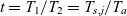
To investigate combined jet temperature–compressibility effects, McGuirk and Feng (Reference McGuirk and Feng18) used the same nozzle as employed in Ref. Reference Feng and McGuirk13 for an under-expanded (NPR = 2.32) jet and for NTRs up to 3.0. Non-dimensional data for the mean centreline axial velocity and turbulence rms are shown in Figs 16 and 17. The oscillations with magnitude of 16–21% of the core velocity identify the region of oblique shock waves as the jet static pressure decreases back to the ambient value. The potential core length clearly shortens while the decay rate steepens as the NTR increases, although these trends cease after NTR = 2.03. The potential core length is increased by jet heating, but less so than it would be in the absence of compressibility. A similar diminishing effect of temperature ratio is visible in the centreline axial turbulence development (Fig. 17); the peak rms increases slightly with the NTR, and its location moves upstream, but once again a temperature effect is not observed above NTR = 2.03.
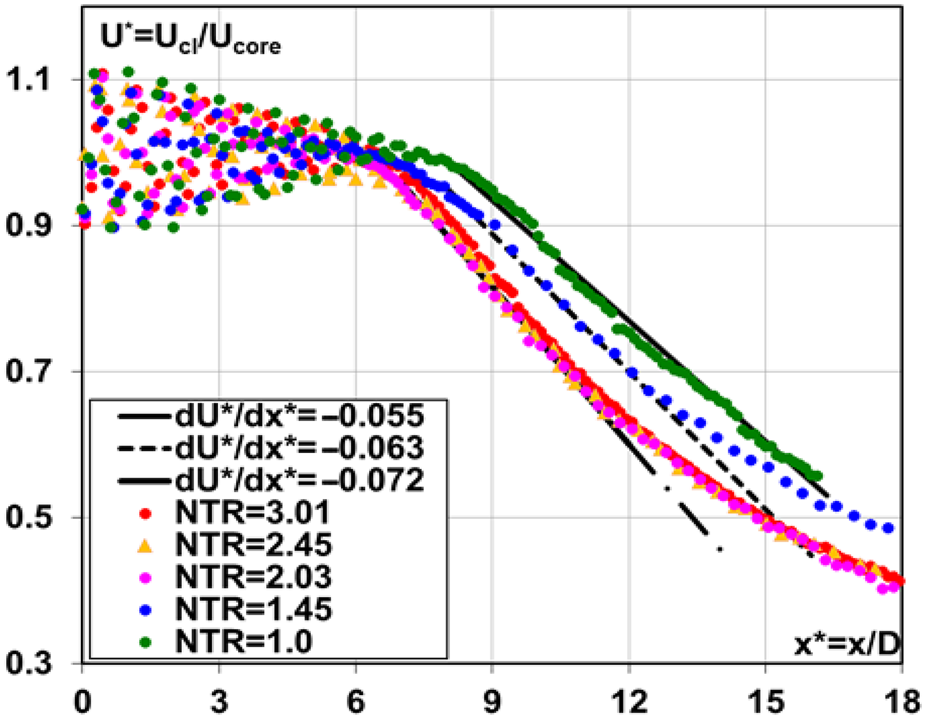
Figure 16. Centreline mean axial velocity at NPR = 2.32 with various NTR from Ref. Reference McGuirk and Feng18.
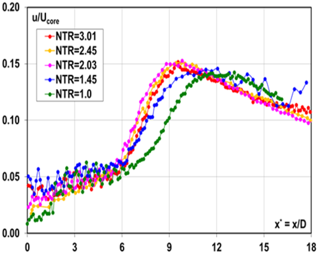
Figure 17. Centreline axial turbulence at NPR = 2.32 with various NTR from Ref. Reference McGuirk and Feng18.
Analysis of radial profiles over the potential core length enables evaluation of the shear-layer growth rate. This and other data on hot jets from the literature have been added to the compressibility reduction diagram in Fig. 15 to obtain Fig. 18. Some data (Fig. 18, black and purple symbols) deviate from the best-fit line identified by the majority of data (Fig. 18, red line, extrapolated for high values of M c parallel to the black line of Ref. Reference Barone, Oberkampf and Blottner12). This best-fit line is supported by a range of measurements taken in different facilities and would appear to be a distinctive feature of jet-related shear layers.
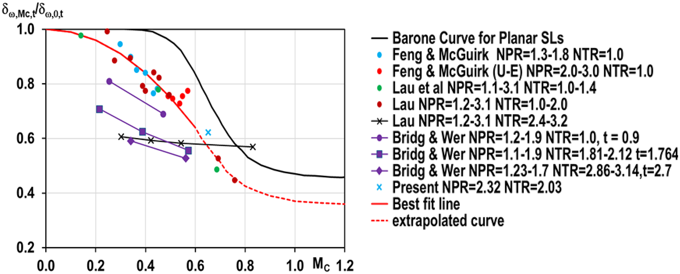
Figure 18. Compressibility-induced growth rate reduction for various NPR and NTR from Ref. Reference McGuirk and Feng18.
Given the importance of the potential core length, an empirical correlation was evaluated in Ref. Reference McGuirk and Feng18 based on the concept of competing compressibility and temperature effects. The correlation derived for the potential core length (L p ) as a function of both M j and t is given in Equation (4) and compared with available data in Fig. 19. Whilst not perfect, the correlation of Equation (4) covers the wide ranges of Mach number and temperature ratio of interest in aerospace engineering and represents a valuable design aid.
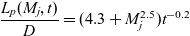 \begin{align}\frac{{{L_p}({M_j},t)}}{D} = (4.3 + M_j^{2.5}){t^{ - 0.2}}\end{align}
Turbulence modelling
The descriptions above highlight the crucial role played by turbulent mixing. Accurate and generally applicable turbulence modelling is essential. Various approaches including RANS, LES and Direct Numerical Simulation (DNS) have all been used for propulsive jet aerodynamics (turbulence modelling impact on aeroacoustics is dealt with in Subsection 2.2). DNS, due to its high mesh dependency on Re, has mainly been applied to canonical flows, for example a low-Re round jet (Re j = 2,000 in Ref. Reference Taub, Lee, Balachandar and Sherif19), and RANS or LES are the principal options.
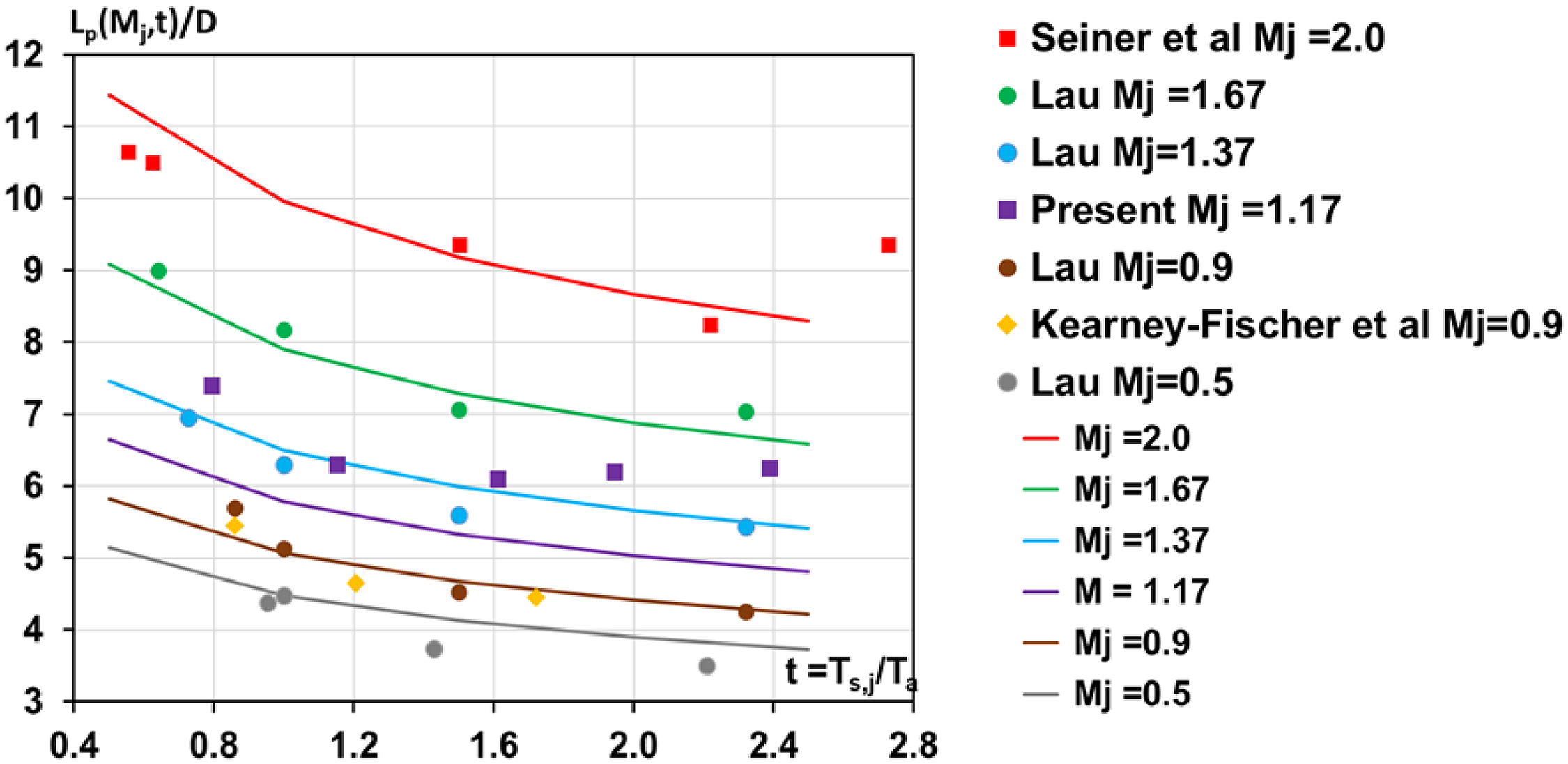
Figure 19. L p (Mj,t) correlation (lines) compared with measurements (symbols) from Ref. Reference McGuirk and Feng18.
The performance of RANS for propulsive jet flows was reviewed in 2006 by Georgiadis and DeBonis (Reference Georgiadis and DeBonis20) and a decade later by Yoder at al. (Reference Yoder, DeBonis and Georgiadis21). The overall conclusion was that standard two-equation models (k–
 $\varepsilon$
, k–
$\varepsilon$
, k–
 $\omega$
etc.) were unable to predict (with the accuracy required by designers) the variation of the potential core length with compressibility, temperature or the 3D nozzle shapes of engineering interest. As noted in Ref. Reference Barone, Oberkampf and Blottner12, attempts to introduce compressibility effects, whilst superficially successful, were based on incorrect physical assumptions. This situation has improved in only one aspect: Gomez et al. (Reference Gomez and Girimaji22) proposed a modified pressure–strain model (in an algebraic stress form of the Reynolds stress transport equations), which correctly reproduced compressibility-induced damping. However, the model has so far not been applied to high-speed jets. Similarly, eddy viscosity model improvements to capture temperature ratio effects have been put forward by Tam and Ganesan (Reference Tam and Ganesan23), Abdol-Hamid et al. (Reference Abdol-Hamid, Paul Pao, Massey and Elmiligui24) and Truemner and Mundt (Reference Truemner and Mundt25). By adding a total temperature gradient correction to the production terms in the turbulence equations, the tendency of the k–ɛ model to overpredict the potential core length and underestimate the turbulence intensity in hot jets was corrected. It is difficult, however, to conclude that this approach has general validity; it is totally empirical with no physically justified basis, simply introducing an ad hoc adjustment. It seems premature to conclude with any confidence that the problem of RANS hot jet modelling has been resolved.
$\omega$
etc.) were unable to predict (with the accuracy required by designers) the variation of the potential core length with compressibility, temperature or the 3D nozzle shapes of engineering interest. As noted in Ref. Reference Barone, Oberkampf and Blottner12, attempts to introduce compressibility effects, whilst superficially successful, were based on incorrect physical assumptions. This situation has improved in only one aspect: Gomez et al. (Reference Gomez and Girimaji22) proposed a modified pressure–strain model (in an algebraic stress form of the Reynolds stress transport equations), which correctly reproduced compressibility-induced damping. However, the model has so far not been applied to high-speed jets. Similarly, eddy viscosity model improvements to capture temperature ratio effects have been put forward by Tam and Ganesan (Reference Tam and Ganesan23), Abdol-Hamid et al. (Reference Abdol-Hamid, Paul Pao, Massey and Elmiligui24) and Truemner and Mundt (Reference Truemner and Mundt25). By adding a total temperature gradient correction to the production terms in the turbulence equations, the tendency of the k–ɛ model to overpredict the potential core length and underestimate the turbulence intensity in hot jets was corrected. It is difficult, however, to conclude that this approach has general validity; it is totally empirical with no physically justified basis, simply introducing an ad hoc adjustment. It seems premature to conclude with any confidence that the problem of RANS hot jet modelling has been resolved.
It is perhaps not surprising that RANS eddy viscosity models experience such difficulties for the present flow type. They are calibrated to match a range of Two-Dimensional (2D) free shear flow experimental data in which turbulent eddies have achieved an asymptotic state of development. The jet near field is far from this, comprising turbulence which originates in a wall-bounded flow and passes through a mixing layer phase, finally experiencing just the preliminary stage of development into a fully formed jet. This problem was recognised in Refs Reference Georgiadis and DeBonis20 and Reference Yoder, DeBonis and Georgiadis21, both of which concluded that the LES approach was more appropriate for flows where the large-scale structures are adjusting rapidly to their changing flow environment.
Doubts were, however, expressed in Refs Reference Georgiadis and DeBonis20 and Reference Yoder, DeBonis and Georgiadis21 regarding the robustness and maturity of several numerical aspects of LES CFD codes. This situation has improved in the intervening period, although access to High-Performance Computing (HPC) facilities and the cost or time resource involved remain significant issues. There is little doubt that LES has been proven a viable option that is capable of overcoming precisely the problems that are so difficult for RANS. McMullan et al. (Reference McMullan, Coats and Gao26) and Wang et al. (Reference Wang, Froelich, Michelassi and Rodi27), for example, show that LES accurately predicts the temperature ratio effect in incompressible planar shear layers and low-Mach-number jets, respectively. Le Ribault (Reference Le Ribault28) presented LES of a spatially developing high-speed planar shear layer at various convective Mach numbers and demonstrated excellent agreement with the data fit recommended by Barone et al. (Reference Barone, Oberkampf and Blottner12), as illustrated in Fig. 20. Bogey and Marsden (Reference Bogey and Marsden29) and DeBonis (Reference DeBonis30) confirmed that, with sufficiently fine meshes, LES performed very well in capturing the near field of single round jets in stagnant surroundings at M j = 0.9. Finally, examples of confidence-building results for LES for temperature effects in subsonic jets have also been reported. The results in Ref. Reference Bogey and Marsden29 did not match the experimental temperature ratios of Bridges (Reference Bridges31) exactly, but the change in the potential core length for hot jets was reproduced. For a temperature ratio of 1.6, the reduction in X pc was 21% (LES) versus 25% (experimentally). Similarly, in Ref. Reference DeBonis30, LES predictions were compared with the data of Bridges (Reference Bridges31) and demonstrated the clear superiority of LES versus RANS, as shown in Fig. 21.
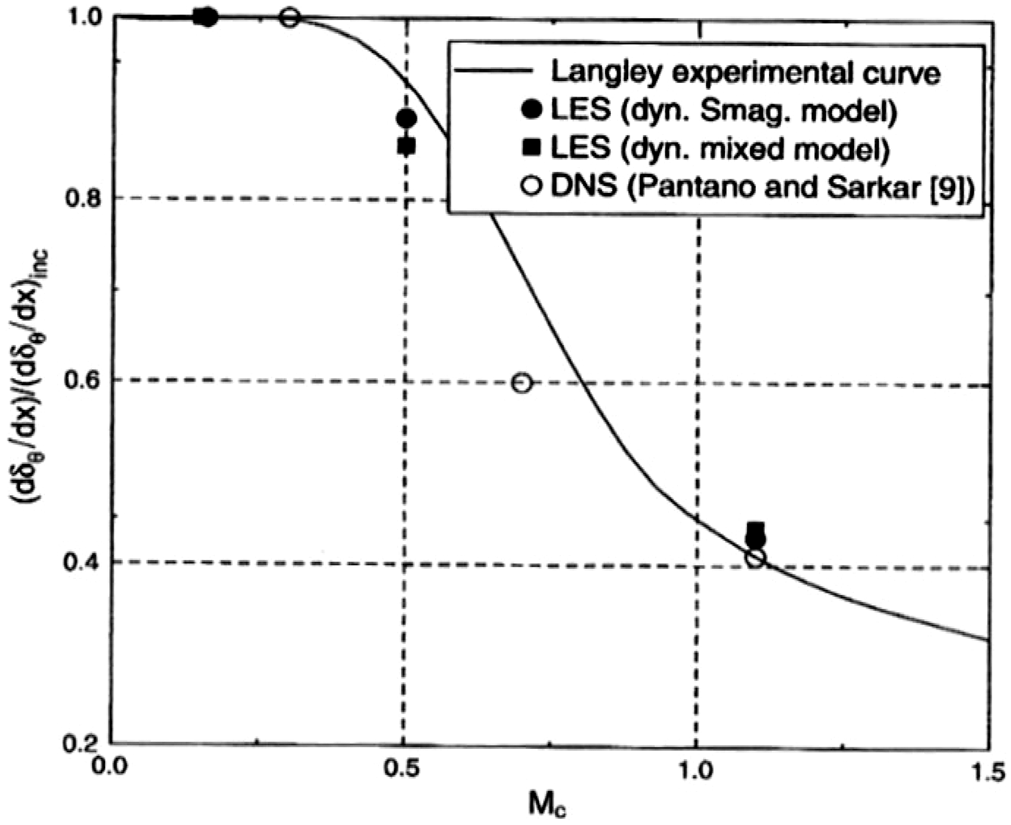
Figure 20. LES prediction of compressibility-based reduction of shear layer growth from Ref. Reference Le Ribault28.
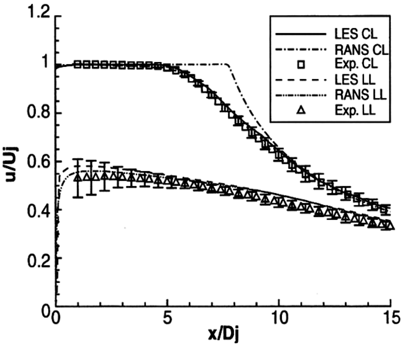
Figure 21. LES, RANS and experimental results for mean axial velocity, centreline/lipline from Ref. Reference DeBonis30.
As noted above, these improvements are accompanied by substantially increased computational cost. The LES mesh size is typically one to two orders of magnitude larger and, unlike in RANS, must increase as Re j increases. In DeBonis (Reference DeBonis30) the mesh comprised 36m points, and Bogey and Marsden (Reference Bogey and Marsden29) employed meshes as large as 250m. LES is also fundamentally an unsteady calculation, requiring perhaps O(105–106) timesteps to calculate statistically stationary values of first/second-order statistics (including a considerable ‘start-up’ time for the initial conditions to be ‘forgotten’). These numbers underline the need for access to large, multi-core HPC facilities for LES. The LES computational time is obviously not compatible with regular, repeated quick-turnaround design explorations. Hence, it is inevitable that RANS will continue to play a role in engineering design for the foreseeable future. LES at present can make its most useful contribution via: (i) helping to devise ways of modifying RANS turbulence models to allow better performance of specific aspects important to the flows considered, and (ii) increasing the precision of predictions for detailed analysis of down-selected concepts at a later stage of the design cycle.
LES mesh design is not as straightforward as for RANS, where regions of high mean spatial gradient are the only criterion. Guidance for LES has been provided by Choi and Moin (Reference Choi and Moin32), with the design strategy based broadly on the assumption that a ‘well-resolved’ LES mesh is one in which the cell size is everywhere able to capture >80% of the time-averaged turbulence energy in the ‘mesh-resolved scales’ (Reference Pope6), that is, <20% is at ‘sub-grid scale’ (SGS) accounted for by an SGS model or by the numerical discretisation scheme. Since the turbulence energy field is unknown before the LES calculation begins, resort has to be made to estimation using, for example, an a priori RANS calculation (Reference Dianat, McGuirk, Fokeer and Spencer33). In addition, constructing well-resolved LES meshes near walls is a considerable challenge, since the energy-containing, dynamically important eddies become smaller as the near-wall viscous region is approached and this feature is exacerbated as Re increases. This has led to the concept of ‘wall-modelled’ LES to avoid the strict near-wall resolution requirement. A popular proposal here is the wall stress approach of Kawai and Larsson (Reference Kawai and Larsson34) where the SGS model is used for all mesh points but the under-resolution of the boundary layer is corrected by imposing a wall-stress boundary condition. This is currently the most favoured approach for handling internal nozzle flow at high Re (Reference Angelino, Xia and Page35).
Finally, a perennial problem with LES, for which no definitive solution yet exists, is proper specification of inflow boundary conditions. Wu (Reference Wu36) and Dhamankar et al. (Reference Dhamankar, Blaisdell and Lyrintzis37) have provided reviews on this subject. Of the methods proposed, two have found application in jet flow applications: Synthetic Turbulence (ST) and the Recycling–Rescaling Method (R2M) The issue addressed is the demand in LES for a time-varying inflow specification comprising a correlated and self-consistent data set for all resolved length/time scales of motion present in the inflow. Incomplete or inconsistent specification results in an ‘adjustment’ length to develop correlated turbulent structures. An example of this in the current context is the specification of flow conditions for an LES calculation beginning at the nozzle exit. The realisation that the details of the initial shear layer development are influenced by the nozzle exit profile resulted in specific measurements being made. Variations in the measured potential core length at different facilities for the same operating conditions are generally believed to be primarily caused by differing nozzle exit profiles.
As noted above, Bridges and Wernet (Reference Bridges and Wernet10) conducted nozzle exit measurements in their creation of a validation data set for subsonic jet noise modelling, although surprisingly none of the published LES studies of the data in Ref. Reference Bridges and Wernet10 have made use of these exit measurements (e.g. Naqavi et al. (Reference Naqavi, Wang, Tucker, Mahak and Strange38)). The ST and R2M techniques allow experimental measurements to be incorporated into LES inlet conditions at various levels of self-consistency. The ST method known as digital filtering has been mainly adopted in LES jet flow predictions (Reference Brés, Jaunet, Le Rallic, Jordan, Colonius and Lele39,Reference Brés, Jordan, Jaunet, Le Rallic, Cavalieri, Towne, Lele, Colonius and Schmidt40), following Klein et al. (Reference Klein, Sadiki and Janicka41) by applying signal modelling techniques to manipulate the coefficients of a linear recursive filter. This creates a time series that is consistent with a specified ‘target’ data set of mean velocities and Reynolds normal stresses (from measurements). Approximations are introduced (principally the need to specify the turbulence length scale distribution and the spatial correlation function shape), hence the correct physical conditions cannot be matched exactly and some adjustment length is inevitable. These approximations are avoided in the R2M approach of Xiao et al. (Reference Xiao, Dianat and McGuirk42). In this technique, an LES solution within an extra ‘precursor’ domain is required. The inflow conditions within this precursor domain are generated by recycling the velocity field (after rescaling) back to the inlet from a user-selected downstream location. When the solution is statistically stationary, the velocity field at the outlet of the precursor domain represents the time-dependent inlet conditions for the main LES solution. In this version of R2M, continued rescaling acts as a forcing method and is applied throughout the precursor domain, whose streamwise dimension is chosen to ensure that turbulence length scales are unconstrained by boundary conditions. Rescaling forces the time-mean velocity and turbulence normal stresses to match user-specified profiles. Note that all the turbulent length scales and spatial (and temporal) correlations are self-generated and consistent with user-specified statistical input data. The disadvantage is that a second LES solution is required with its attendant cost. Figure 22 provides examples of this method’s ability to: (i) capture specified mean and turbulent stress profiles, and (ii) create shear stress/axial length scale profiles in agreement with experiments although not part of the user input. Examples of application to a nozzle flow are presented in Subsection 3.2.
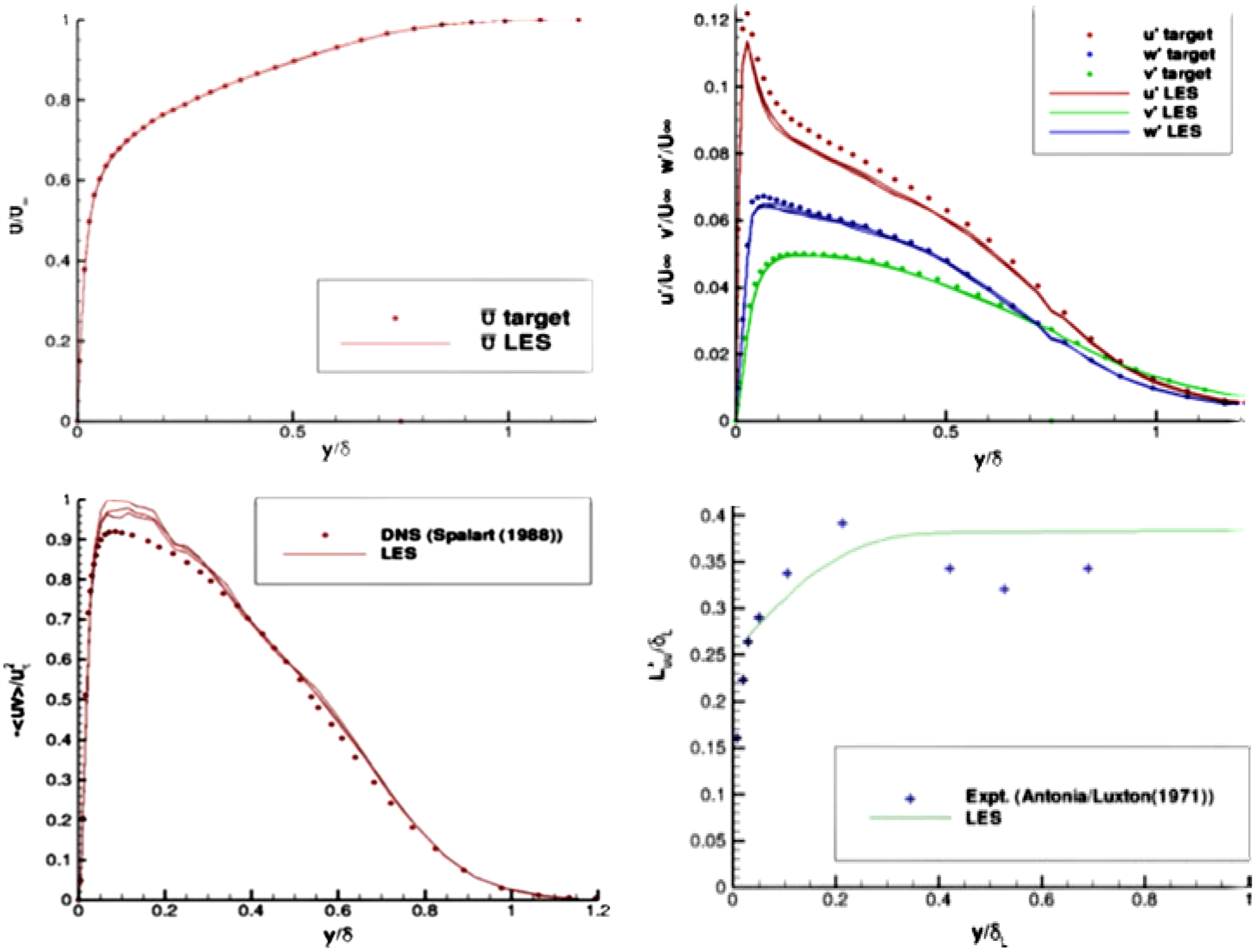
Figure 22. R2M-generated inlet boundary layer profiles from Ref. Reference Xiao, Dianat and McGuirk42: mean axial velocity and rms turbulence (top) and shear stress and integral length scale (bottom).
2.2 Aeroacoustic aspects
Over the last 20 years, a transition from RANS-based to LES-based modelling has also begun in aeroacoustics; not a total shift, but rather a trend for increased use of LES is clear. Lighthill’s pioneering work (Reference Lighthill4) on propagation to the far field (where noise levels are regulated) of acoustic pressure fluctuations proposed a modification of the Navier–Stokes equations to have a left-hand side representing a homogeneous wave equation (pressure wave propagation at the ambient speed of sound) and a right-hand side viewed as acoustic noise sources. Further manipulation demonstrated (in a subsonic unheated jet, for example) that the far-field acoustic pressure intensity was defined by the volume integral of the fourth-order time derivative of the two-point two-time correlation of the fluctuating Reynolds stress tensor; this is defined in Equation (5) with and
 $\underline{\eta}$
spatial and τ temporal separations and the dash superscript indicating a turbulent velocity fluctuation:
$\underline{\eta}$
spatial and τ temporal separations and the dash superscript indicating a turbulent velocity fluctuation:
 \begin{align} r_{ij,kl} (\underline{x}, \underline{\eta} , {\tau})= \overline{[u^{\prime}_{i} u^{\prime}_{j} - \overline{u^{\prime}_{i} u^{\prime}_{j}}] (\underline{x},t)[u^{\prime}_{k} u^{\prime}_{l} - \overline{u^{\prime}_{k} u^{\prime}_{l}}] ({\underline{x}} + {\underline{\eta}} , t + {\tau})} \end{align}
Morris and Farassat (Reference Morris and Farassat43) pointed out that assumptions about this property are an inherent part of all RANS-based jet noise models. If a physically accurate specification of the acoustic source term can be identified, solution of the wave equation using Green’s function techniques establishes the far-field sound.
In general, the approach taken has been to express the non-dimensional form of
 ${r_{ij,kl}}$
(
${r_{ij,kl}}$
(
 ${R_{ij,kl}}$
) via a correlation ‘shape function’ and recover the dimensional quantity at any point in the flow by multiplying by a local characteristic turbulence velocity scale raised to the fourth power. Guidance regarding the form of the shape function was sought from experimental measurements of space–time correlations. Initially (Reference Fisher and Davies44) these were undertaken using multiple hot-wire probes, but only for the second-order correlation
${R_{ij,kl}}$
) via a correlation ‘shape function’ and recover the dimensional quantity at any point in the flow by multiplying by a local characteristic turbulence velocity scale raised to the fourth power. Guidance regarding the form of the shape function was sought from experimental measurements of space–time correlations. Initially (Reference Fisher and Davies44) these were undertaken using multiple hot-wire probes, but only for the second-order correlation
 ${R_{ij}}(\underline x ,\underline \eta ,\tau )$
, and only for a few components and separation directions. Later, this was extended to measurements of fourth-order correlations, but again only for a restricted set and only in a round jet (Reference Morris and Zaman45). Typically, exponential or Gaussian shape functions have been used, with arguments
${R_{ij}}(\underline x ,\underline \eta ,\tau )$
, and only for a few components and separation directions. Later, this was extended to measurements of fourth-order correlations, but again only for a restricted set and only in a round jet (Reference Morris and Zaman45). Typically, exponential or Gaussian shape functions have been used, with arguments
 $(\underline x ,\underline \eta ,\tau )$
again made dimensionless using assumed local turbulence length/time scales. RANS turbulence predictions have typically been used to provide the variation throughout the jet of these turbulence scales (e.g. for the k–ɛ model, the velocity, length and time scales are
$(\underline x ,\underline \eta ,\tau )$
again made dimensionless using assumed local turbulence length/time scales. RANS turbulence predictions have typically been used to provide the variation throughout the jet of these turbulence scales (e.g. for the k–ɛ model, the velocity, length and time scales are
 ${k^{^{{\raise0.5ex\hbox{$\scriptstyle 1$}\kern-0.1em/\kern-0.15em\lower0.25ex\hbox{$\scriptstyle 2$}}}}},\,{k^{^{{\raise0.5ex\hbox{$\scriptstyle 3$}\kern-0.1em/\kern-0.15em\lower0.25ex\hbox{$\scriptstyle 2$}}}}}/\varepsilon ,\,k/\varepsilon $
). Empirical coefficients to control the correlation magnitude and the assumed turbulence scales were introduced and adjusted to optimise accuracy. Reliance on a restricted set of measurements makes it difficult to apply this approach to other geometries/flow conditions. To address this problem, Karabasov et al. (Reference Karabasov, Afsar, Hynes, Dowling, McMullan, Pokora, Page and McGuirk46) proposed that the coefficients of the turbulence length/time scales should not be determined empirically but rather selected on the basis of information on turbulence scales taken from an LES solution. Confidence that LES can provide accurate predictions of space–time correlations was provide using the time-resolved Stereoscopic Particle Image Velocimetry (SPIV) data of Pokora and McGuirk (Reference Pokora and McGuirk47). Figure 23(a) indicates how the largest correlation (
${k^{^{{\raise0.5ex\hbox{$\scriptstyle 1$}\kern-0.1em/\kern-0.15em\lower0.25ex\hbox{$\scriptstyle 2$}}}}},\,{k^{^{{\raise0.5ex\hbox{$\scriptstyle 3$}\kern-0.1em/\kern-0.15em\lower0.25ex\hbox{$\scriptstyle 2$}}}}}/\varepsilon ,\,k/\varepsilon $
). Empirical coefficients to control the correlation magnitude and the assumed turbulence scales were introduced and adjusted to optimise accuracy. Reliance on a restricted set of measurements makes it difficult to apply this approach to other geometries/flow conditions. To address this problem, Karabasov et al. (Reference Karabasov, Afsar, Hynes, Dowling, McMullan, Pokora, Page and McGuirk46) proposed that the coefficients of the turbulence length/time scales should not be determined empirically but rather selected on the basis of information on turbulence scales taken from an LES solution. Confidence that LES can provide accurate predictions of space–time correlations was provide using the time-resolved Stereoscopic Particle Image Velocimetry (SPIV) data of Pokora and McGuirk (Reference Pokora and McGuirk47). Figure 23(a) indicates how the largest correlation (
 ${R_{11,11}}$
) varies with separation in both the x direction and time (
${R_{11,11}}$
) varies with separation in both the x direction and time (
 $\tau$
). The diagonal trajectory of the peak correlation indicates the eddy convection velocity (
$\tau$
). The diagonal trajectory of the peak correlation indicates the eddy convection velocity (
 $\sim$
0.6U
j
). The SPIV data revealed significant values of many components of
$\sim$
0.6U
j
). The SPIV data revealed significant values of many components of
 ${R_{ij,kl}}(\underline x ,\underline \eta ,\tau )$
. The 81 components of the fourth-order tensor reduce with symmetry to 36, all of which were measured in Ref. Reference Lyrintzis and Coderoni48. Figure 23(b) presents the ratio of the peak amplitude of three components relative to the largest along the centreline, showing non-negligible values; even in an axisymmetric jet, many components are significant. Finally, Fig. 24, using SPIV data from Ref. Reference Pokora and McGuirk47, confirms that LES predicts high-order correlations accurately for second- and fourth-order spatio-temporal correlations.
${R_{ij,kl}}(\underline x ,\underline \eta ,\tau )$
. The 81 components of the fourth-order tensor reduce with symmetry to 36, all of which were measured in Ref. Reference Lyrintzis and Coderoni48. Figure 23(b) presents the ratio of the peak amplitude of three components relative to the largest along the centreline, showing non-negligible values; even in an axisymmetric jet, many components are significant. Finally, Fig. 24, using SPIV data from Ref. Reference Pokora and McGuirk47, confirms that LES predicts high-order correlations accurately for second- and fourth-order spatio-temporal correlations.
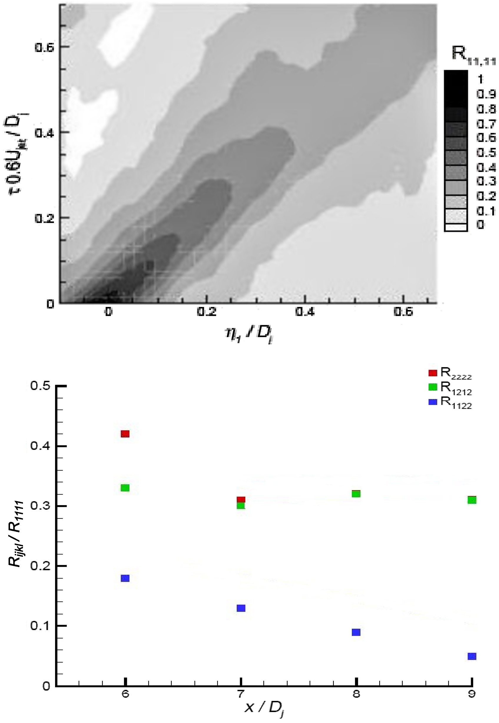
Figure 23. SPIV measured spatio-temporal correlation map for
 ${R_{11,11}}$
at (4D
j
, 0.5D
j
, 00) (top) and centreline variation of SPIV measured peak values relative to
${R_{11,11}}$
at (4D
j
, 0.5D
j
, 00) (top) and centreline variation of SPIV measured peak values relative to
 ${R_{11,11}}$
(bottom) from Ref. Reference Pokora and McGuirk47.
${R_{11,11}}$
(bottom) from Ref. Reference Pokora and McGuirk47.
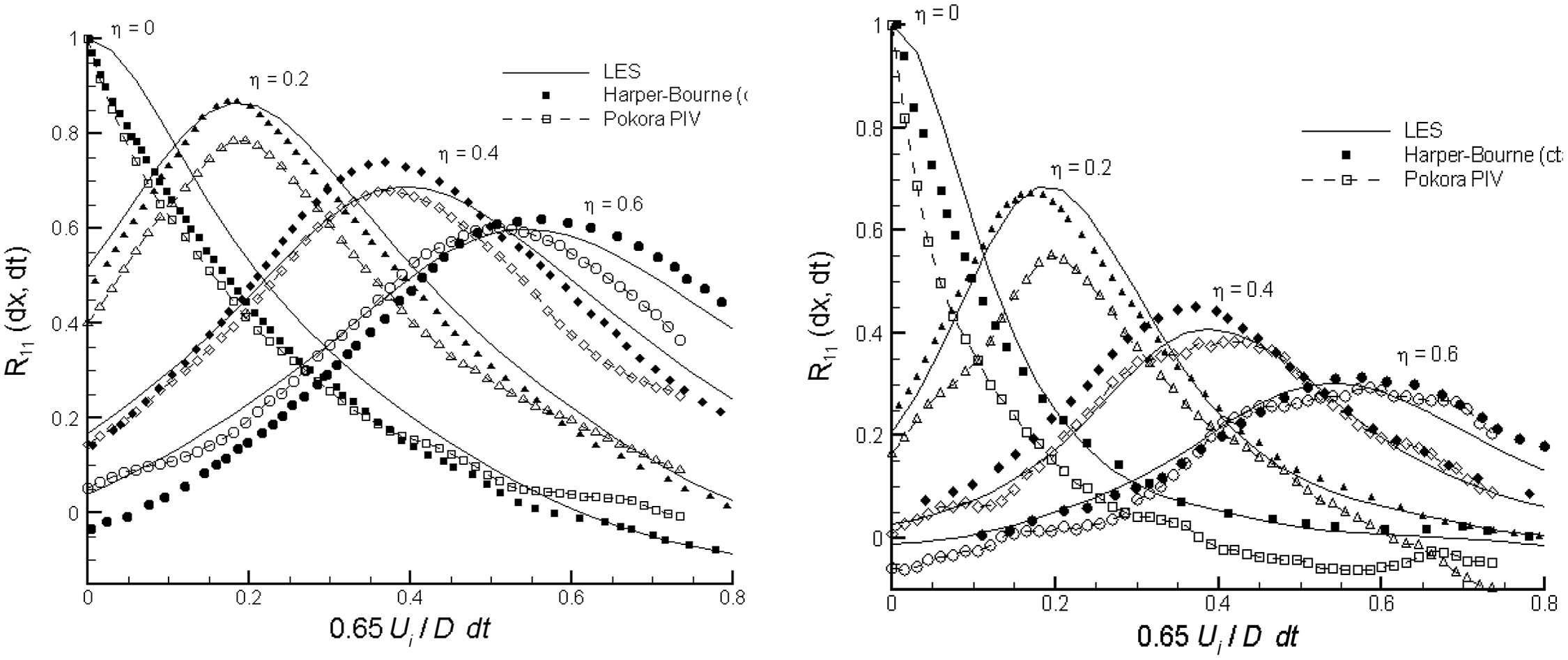
Figure 24. Comparison of LES predictions with measurements of Ref. Reference Pokora and McGuirk47
 ${R_{11}}$
and
${R_{11}}$
and
 ${R_{1111}}$
from Ref. Reference Karabasov, Afsar, Hynes, Dowling, McMullan, Pokora, Page and McGuirk46.
${R_{1111}}$
from Ref. Reference Karabasov, Afsar, Hynes, Dowling, McMullan, Pokora, Page and McGuirk46.
Following the procedure outlined above, RANS turbulence scales were manipulated in Ref. Reference Karabasov, Afsar, Hynes, Dowling, McMullan, Pokora, Page and McGuirk46 using LES information from Ref. Reference Pokora and McGuirk47. The method was then able to predict noise measurements at both peak noise (30°) and sideline (90°) angles, as shown in Fig. 25; this had not previously been possible with RANS-based methods.
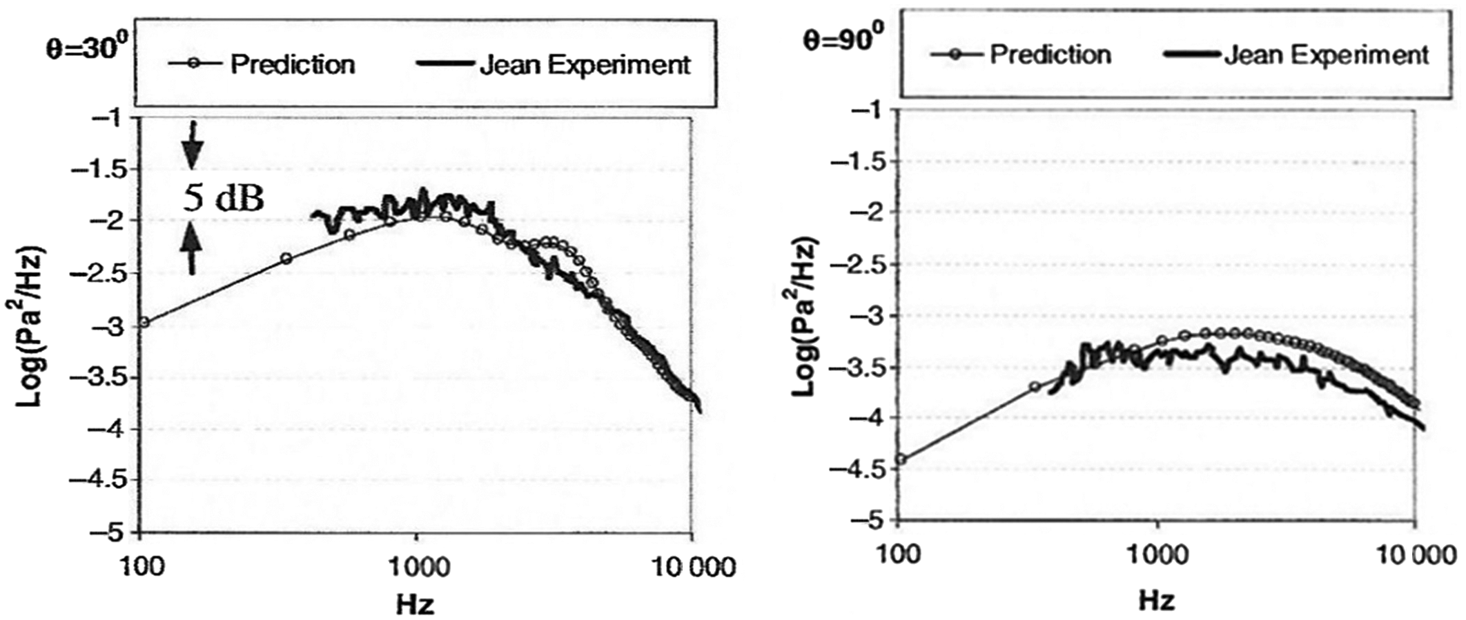
Figure 25. Noise spectra comparison between RANS-based method and experiments at two angles from Ref. Reference Karabasov, Afsar, Hynes, Dowling, McMullan, Pokora, Page and McGuirk46.
There is, in principle, no reason why LES could not be used to capture both turbulent sources and propagation to the far field. However, since this lies
 $\sim$
50–75D away from the jet and LES is computationally expensive, such so-called direct LES computation of noise is likely to be prohibitively expensive and is not widely adopted, particularly for cases with complex geometry. The numerical techniques most widely used for LES complex applications are typically a blended mixture of second-order upwind and second-order central schemes, which are robust and have sufficiently low dissipation for turbulent flow, although not for wave propagation over long distances. A hybrid approach using one method for turbulence capture and another best suited to propagation is more appropriate.
$\sim$
50–75D away from the jet and LES is computationally expensive, such so-called direct LES computation of noise is likely to be prohibitively expensive and is not widely adopted, particularly for cases with complex geometry. The numerical techniques most widely used for LES complex applications are typically a blended mixture of second-order upwind and second-order central schemes, which are robust and have sufficiently low dissipation for turbulent flow, although not for wave propagation over long distances. A hybrid approach using one method for turbulence capture and another best suited to propagation is more appropriate.
A survey of all aspects of the application of LES to jet aeroacoustics has been provided by Lyrintzis and Coderoni (Reference Lyrintzis and Coderoni48). For the current purposes, it is sufficient to note that two techniques for propagation to the far field have been considered. The first is a surface-based technique such as the Linear Euler Equation (LEE) solver (Reference Bogey and Marsden49) or the Ffowcs Williams–Hawkings (FWH) approach (Reference Ffowcs Williams and Hawkings50); these are broadly equivalent, although the FWH approach is by far the more popular. LES information is extracted on a surface surrounding (and entirely enclosing) the turbulent noise sources and provides an interface to the propagation technique. The second technique is Acoustic Perturbation Equations (APE) proposed by Ewart and Schroeder (Reference Ewart and Schroeder51) (some promising results from this method (Reference Moratilla-Vega, Lackhove, Janicka, Xia and Page52) are shown in Section 3). The APE approach also follows Lighthill’s original idea but manipulates the governing equations into an LEE LHS and a RHS interpreted as a source vector for the LEE system, exciting vortical, entropic and acoustic modes. These equations are modified into an APE format by filtering the RHS source terms so that only acoustic modes appear. One important numerical property thereby introduced is the elimination of vortical modes which occur as instabilities in the LEE system. Note that APE is a volume rather than a surface method; the APE equations are solved in the entire region from near to far field.
The hybrid concept is illustrated in Fig. 26, which presents results from the LES/LEE approach of Ref. Reference Bogey and Marsden49 for a round jet at M
j
= 0.9 and Re
j
= 105 with a static temperature ratio of 1.0 (FWH would produce similar results). The inner domain contains the jet (identified by fluctuating vorticity contours), while the outer LEE domain shows pressure fluctuation waves. The different discretisation requirements are indicated by the mesh sizes used (1Bn for LES, 1.8Bn for LEE in a study especially focussed on mesh density effects). The typical turbulent subsonic jet noise directivity pattern appears, with noise amplitude largest at an angle of
 $\sim$
30° to the jet axis. The interface surface enclosing the jet must be located with care. The jet pressure field consists of two components: hydrodynamic and acoustic. The acoustic part is defined via the property that it decays with distance following the law of geometrical acoustic spreading (inverse square law). The hydrodynamic part is linked to the turbulent vortical structures, which propagate at their convective speed (proportional to U
j
; see Fig. 23 (top)). The hydrodynamic component is dominant in the jet region but is evanescent, decaying exponentially with distance from the jet. Optimum placement of the surface involves a difficult trade-off as too close means that some noise sources are not LES resolved whereas too far will result in some acoustic propagation being resolved by the less appropriate LES mesh and numerics. Note that this difficulty is circumvented by the APE method, results from which are shown in Section 3.
$\sim$
30° to the jet axis. The interface surface enclosing the jet must be located with care. The jet pressure field consists of two components: hydrodynamic and acoustic. The acoustic part is defined via the property that it decays with distance following the law of geometrical acoustic spreading (inverse square law). The hydrodynamic part is linked to the turbulent vortical structures, which propagate at their convective speed (proportional to U
j
; see Fig. 23 (top)). The hydrodynamic component is dominant in the jet region but is evanescent, decaying exponentially with distance from the jet. Optimum placement of the surface involves a difficult trade-off as too close means that some noise sources are not LES resolved whereas too far will result in some acoustic propagation being resolved by the less appropriate LES mesh and numerics. Note that this difficulty is circumvented by the APE method, results from which are shown in Section 3.
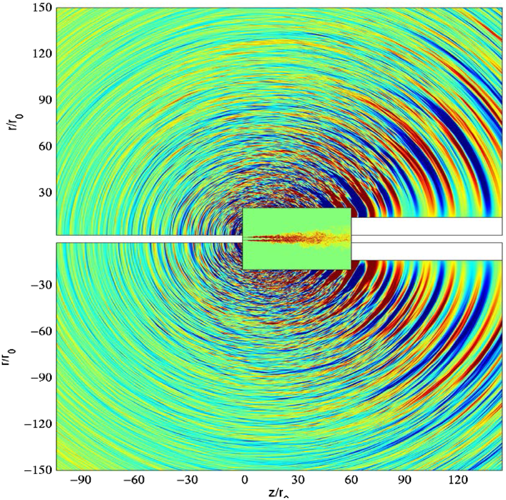
Figure 26. Coupled LES (inner) jet domain and LEE (outer) acoustic propagation domain from Ref. Reference Bogey and Marsden49.
Additional LES numerical issues which influence noise prediction are related to mesh size/time step. The spectrum of frequencies (f) targeted for capture covers the Strouhal number (St) range of 0.01–10 (St = fD j /U j ). The LES grid resolution and time step limit high-frequency capture and accuracy, whereas low-frequency accuracy is determined by the length of the simulation record (accurate statistical sampling of large-eddy dynamics). However, reducing the cell size and time step have a dramatic effect on the computational cost; typically, doubling the highest St resolved increases the computational cost by a factor of 16 (the mesh increasing by 8× and Δt halved). There is the risk that higher frequencies are captured but that the computational time for adequate sampling of low-frequency events becomes unaffordable.
To illustrate the effect of grid refinement on high-frequency noise predictions, results from the LES/FWH study of Angelino et al. (Reference Angelino, Xia and Page53) are shown for a round nozzle at M j = 0.9 and Re j = 106 in Fig. 27. Two LES meshes of 10 × 106 and 80 × 106 cells are compared. The top images show vorticity and pressure contours, with the finer grid (right) demonstrating more small-scale vortex structures and shorter-wavelength sound waves appearing. To focus particular attention on higher-frequency content, a Fourier analysis of the fluctuating pressure field was carried out to examine the dissipative effect of coarser grids. Results for a Strouhal number of 2.0 are shown in the bottom two images (images for St < 1.0 produced two images in close agreement). For St = 2.0, it is clear that, on the coarser mesh (left), the high-frequency noise is unable to propagate far outside the jet edge before it is dissipated.
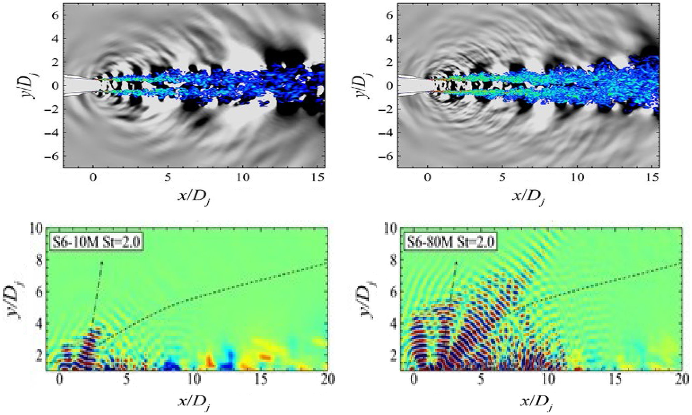
Figure 27. Near-field vorticity/acoustic fields (top) and St = 2.0 pressure fluctuations (bottom) from Ref. Reference Angelino, Xia and Page53.
2.3 Summary
The reviews in Subsections 2.1 and 2.2 have outlined the important, and challenging, aerodynamic and aeroacoustic characteristics of propulsive jets. Experimental measurements representing relevant but fundamentally simple test cases and the performance of various computational techniques proposed for modelling have also been outlined. The following Sections 3 and 4 are intended to illustrate the progress that has been made in validating and assessing modelling developments against measurement data taken in a series of flow scenarios of increasing complexity, moving ever closer to realistic application examples. Section 3 is focussed on civil and Section 4 on military applications.
3.0 Civil aerospace applications
3.1 Cold and hot single jet in stagnant surroundings
The most basic test cases for civil aerospace comprise the near-field aerodynamics and far-field acoustic signature of single round unheated (static temperature ratio 0.84) or heated (ratio = 2.7) jets in stagnant surroundings at high Re
j
(
 $\sim$
105) and high subsonic M
j
(0.9). Figures 28 and 29 provide examples of computational studies of this problem compared against flow and acoustic data from Bridges and Wernet (Reference Bridges and Wernet10) and Brown and Bridges (Reference Brown and Bridges54). Two computational techniques are contrasted, both combining LES and FWH methods. Naqavi et al. (Reference Naqavi, Wang, Tucker, Mahak and Strange38) opted for a combined RANS–LES approach where the RANS equations are solved internal to and surrounding the nozzle wall and gradually blended into an LES region where 48m cells were used. Angelino et al. (Reference Angelino, Xia and Page53) retained LES for both the internal nozzle (wall stress model) and jet flow and carried out a grid resolution study (with 5–80m cells) to explore the effect of finer meshes on flow/noise predictions. Both FWH treatments chose similarly located noise source containing surfaces and applied averaging or filtering over multiple ‘end plates’ to remove pseudo-sound generated by vortical structures crossing the FWH surface. Results from Ref. Reference Naqavi, Wang, Tucker, Mahak and Strange38 for the unheated jet in Fig. 28 (left) indicate an underpredicted potential core length, presumably due to the RANS nozzle treatment since this is captured better by the full LES approach of Ref. Reference Angelino, Xia and Page53 (right) on finer meshes where only 40 and 80m cell meshes capture the centreline development accurately. Both methods provide similar descriptions for axial turbulent rms, with the finer meshes of Ref. Reference Angelino, Xia and Page53 providing more accurate results in the first 10D, but still underpredicting slightly thereafter. The trend effect of jet heating is captured in the work of Ref. Reference Naqavi, Wang, Tucker, Mahak and Strange38 in Fig. 28 (left), reproducing the shortening of the potential core length and the upstream shift of the turbulence peak; quantitatively, however, these effects are overpredicted.
$\sim$
105) and high subsonic M
j
(0.9). Figures 28 and 29 provide examples of computational studies of this problem compared against flow and acoustic data from Bridges and Wernet (Reference Bridges and Wernet10) and Brown and Bridges (Reference Brown and Bridges54). Two computational techniques are contrasted, both combining LES and FWH methods. Naqavi et al. (Reference Naqavi, Wang, Tucker, Mahak and Strange38) opted for a combined RANS–LES approach where the RANS equations are solved internal to and surrounding the nozzle wall and gradually blended into an LES region where 48m cells were used. Angelino et al. (Reference Angelino, Xia and Page53) retained LES for both the internal nozzle (wall stress model) and jet flow and carried out a grid resolution study (with 5–80m cells) to explore the effect of finer meshes on flow/noise predictions. Both FWH treatments chose similarly located noise source containing surfaces and applied averaging or filtering over multiple ‘end plates’ to remove pseudo-sound generated by vortical structures crossing the FWH surface. Results from Ref. Reference Naqavi, Wang, Tucker, Mahak and Strange38 for the unheated jet in Fig. 28 (left) indicate an underpredicted potential core length, presumably due to the RANS nozzle treatment since this is captured better by the full LES approach of Ref. Reference Angelino, Xia and Page53 (right) on finer meshes where only 40 and 80m cell meshes capture the centreline development accurately. Both methods provide similar descriptions for axial turbulent rms, with the finer meshes of Ref. Reference Angelino, Xia and Page53 providing more accurate results in the first 10D, but still underpredicting slightly thereafter. The trend effect of jet heating is captured in the work of Ref. Reference Naqavi, Wang, Tucker, Mahak and Strange38 in Fig. 28 (left), reproducing the shortening of the potential core length and the upstream shift of the turbulence peak; quantitatively, however, these effects are overpredicted.

Figure 28. LES axial velocity and turbulence rms compared with experiments of Refs Reference Bridges and Wernet10, Reference Morris and Zaman45: cold and hot (static temperature ratio = 2.7) jets (left) from Ref. Reference Naqavi, Wang, Tucker, Mahak and Strange38 and cold M j = 0.9 jet (right) from Ref. Reference Angelino, Xia and Page53.
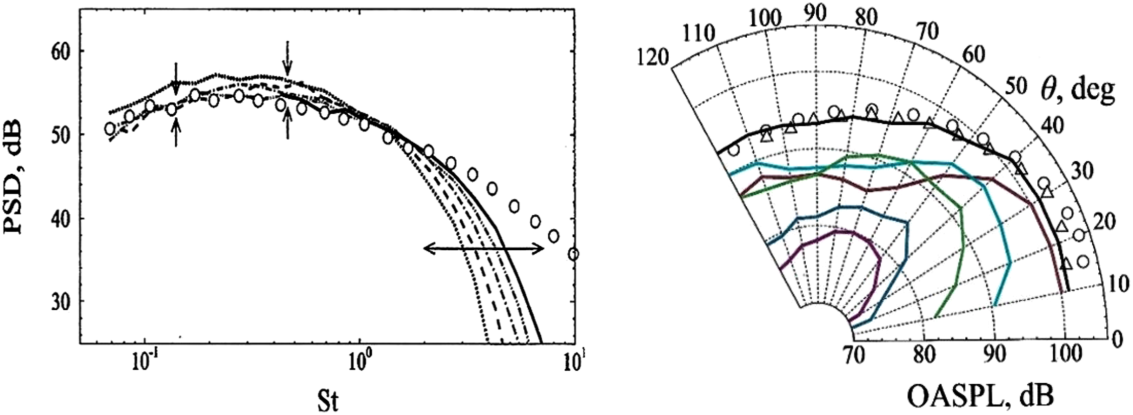
Figure 29. LES/FWH-predicted far-field PSD at
 $\theta\,=\,90^{\circ}$
compared with experiments of Ref. Reference Brown and Bridges54 from Ref. Reference Angelino, Xia and Page53 (left). LES/FWH-predicted OASPL compared with experiments of Refs Reference Tanna17, Reference Brown and Bridges54 from Ref. Reference Angelino, Xia and Page53 (right).
$\theta\,=\,90^{\circ}$
compared with experiments of Ref. Reference Brown and Bridges54 from Ref. Reference Angelino, Xia and Page53 (left). LES/FWH-predicted OASPL compared with experiments of Refs Reference Tanna17, Reference Brown and Bridges54 from Ref. Reference Angelino, Xia and Page53 (right).
The far-field acoustic predictions are similar in both studies (being slightly better for the full LES model), with the trend when changing from a cold to a hot jet shown to be captured well by Ref. Reference Naqavi, Wang, Tucker, Mahak and Strange38. Figure 29 (left) shows a comparison from Ref. Reference Angelino, Xia and Page53 between the predicted and measured Power Spectral Density (PSD) of the sound field at a polar angle of
 $\theta\,=\,90^{\circ}$
(the sideline direction). The agreement is good for all meshes up to a maximum non-dimensional frequency (Strouhal number St) of
$\theta\,=\,90^{\circ}$
(the sideline direction). The agreement is good for all meshes up to a maximum non-dimensional frequency (Strouhal number St) of
 $\sim$
1.5. Greater mesh density improves the capture of lower-frequency amplitude by
$\sim$
1.5. Greater mesh density improves the capture of lower-frequency amplitude by
 $\sim$
1dB, but mesh refinement is more important for higher frequencies. The improvement is, however, rather slow: an increase in mesh density from 20 to 80 × 106 cells only improves the high- frequency capability by a factor of 2 (Stmax from 1.5 to 3). Note also that the finest mesh prediction is only plotted for St
$\sim$
1dB, but mesh refinement is more important for higher frequencies. The improvement is, however, rather slow: an increase in mesh density from 20 to 80 × 106 cells only improves the high- frequency capability by a factor of 2 (Stmax from 1.5 to 3). Note also that the finest mesh prediction is only plotted for St
 $\sim$
0.4 and above. This calculation could not be run for long enough to capture statistically stationary results at lower frequencies.
$\sim$
0.4 and above. This calculation could not be run for long enough to capture statistically stationary results at lower frequencies.
As seen below, this high-frequency issue affects all LES/FWH acoustic predictions and prompted a proposal in Ref. Reference Angelino, Xia and Page53 for the need for a ‘spectral broadening’ approach, that is, to combine noise spectra from simulations with different spatial and temporal resolution, although this would need to be done with some care to ensure consistency in the frequency region where LES solutions overlapped. A directivity map from Ref. Reference Angelino, Xia and Page53 showing the Overall Sound Pressure Level (OASPL) at different polar angles compared with measurements from Refs Reference Tanna17 and Reference Brown and Bridges54 is presented in Fig. 29 (right). The black line corresponds to the total signal, and the coloured lines to different azimuthal modes; lower-order modes (e.g. axisymmetric, m = 0) contribute most at polar angles close to the jet axis, but modes up to m = 7 are significant at larger polar angles, in good agreement with measurements.
To examine whether the FWH procedure may be contributing to the high-frequency problem, Moratilla-Vega et al. (Reference Moratilla-Vega, Lackhove, Janicka, Xia and Page52) used the same LES as in Ref. Reference Angelino, Xia and Page53 but replaced the FWH element with the APE approach of Ref. Reference Ewart and Schroeder51, applying this to the same experimental test case as above. An LES mesh of 25 × 106 cells and an APE mesh of 4 × 10⁶ cells were used (note that fifth-order methods are used in the APE code, see Ref. Reference Moratilla-Vega, Lackhove, Janicka, Xia and Page52). The pressure perturbation fields extracted from the LES/FWH and LES/APE solutions are shown in Fig. 30. The longer wavelengths at low polar angles and the peak directivity angle are similar when using both methods, but the enhanced higher-frequency content in the APE solution is evident, particularly at higher polar angles. Figure 31 examines the predicted far-field PSD at
 $\theta\,=\,90^{\circ}$
obtained from the two methods (one-third octave filtered); the LES/FWH data are shown by solid lines, and the LES/APE results by dashed lines. Two lines are shown for coarse (6.4/1m for LES/APE) and fine (25/4m) meshes. The LES/FWH results are lower than the data shown in Fig. 29 (left) due to the reduced mesh resolution. Note, however, that the LES/APE results are much closer to the measurements, and although the ‘fall-off’ at higher frequency is still noticeable, this is at an increased level of St, indicating a benefit of the higher-order discretisation method adopted in the APE code. Similar benefits are observed in the OASPL plot shown in Fig. 31 (right). Further exploration of the APE method is clearly justified.
$\theta\,=\,90^{\circ}$
obtained from the two methods (one-third octave filtered); the LES/FWH data are shown by solid lines, and the LES/APE results by dashed lines. Two lines are shown for coarse (6.4/1m for LES/APE) and fine (25/4m) meshes. The LES/FWH results are lower than the data shown in Fig. 29 (left) due to the reduced mesh resolution. Note, however, that the LES/APE results are much closer to the measurements, and although the ‘fall-off’ at higher frequency is still noticeable, this is at an increased level of St, indicating a benefit of the higher-order discretisation method adopted in the APE code. Similar benefits are observed in the OASPL plot shown in Fig. 31 (right). Further exploration of the APE method is clearly justified.
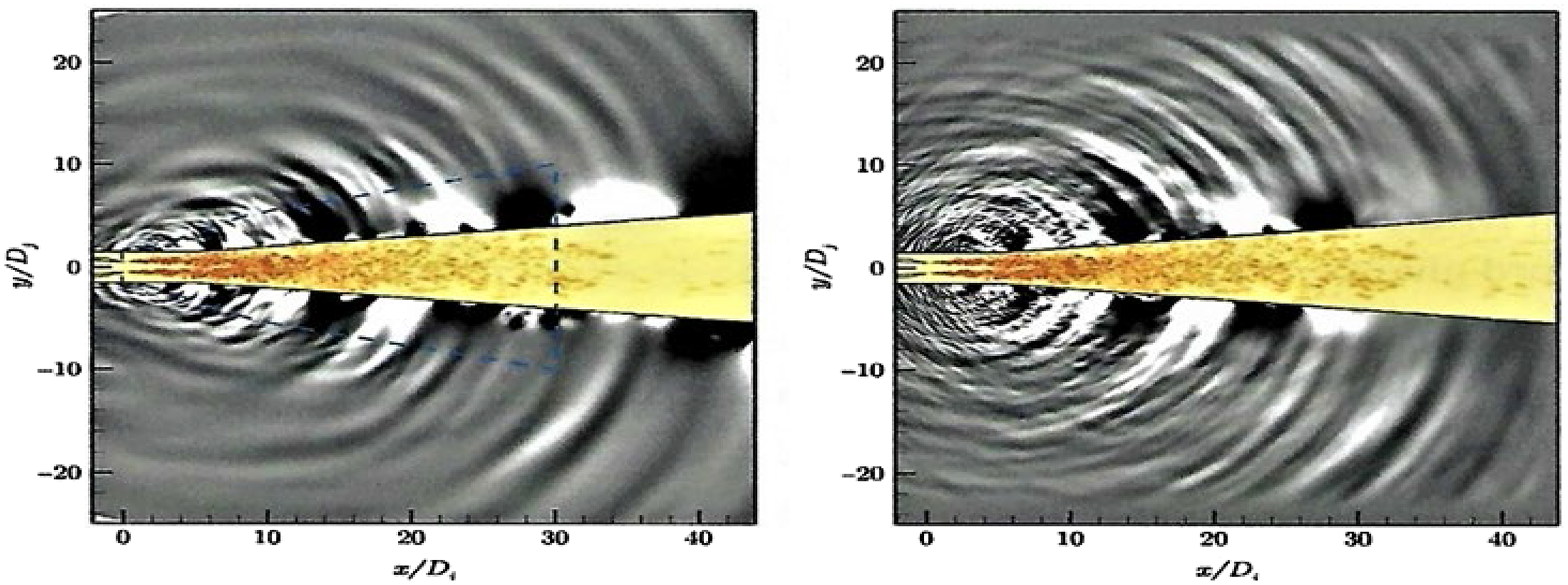
Figure 30. LES/FWH (left) and APE (right) predictions for round jet at M j = 0.9 with static temperature ratio of 0.84. Vorticity and pressure poerturbation contours: LES 25 × 106 cells, APE 4 × 10⁶ cells. From Ref. Reference Moratilla-Vega, Lackhove, Janicka, Xia and Page52.
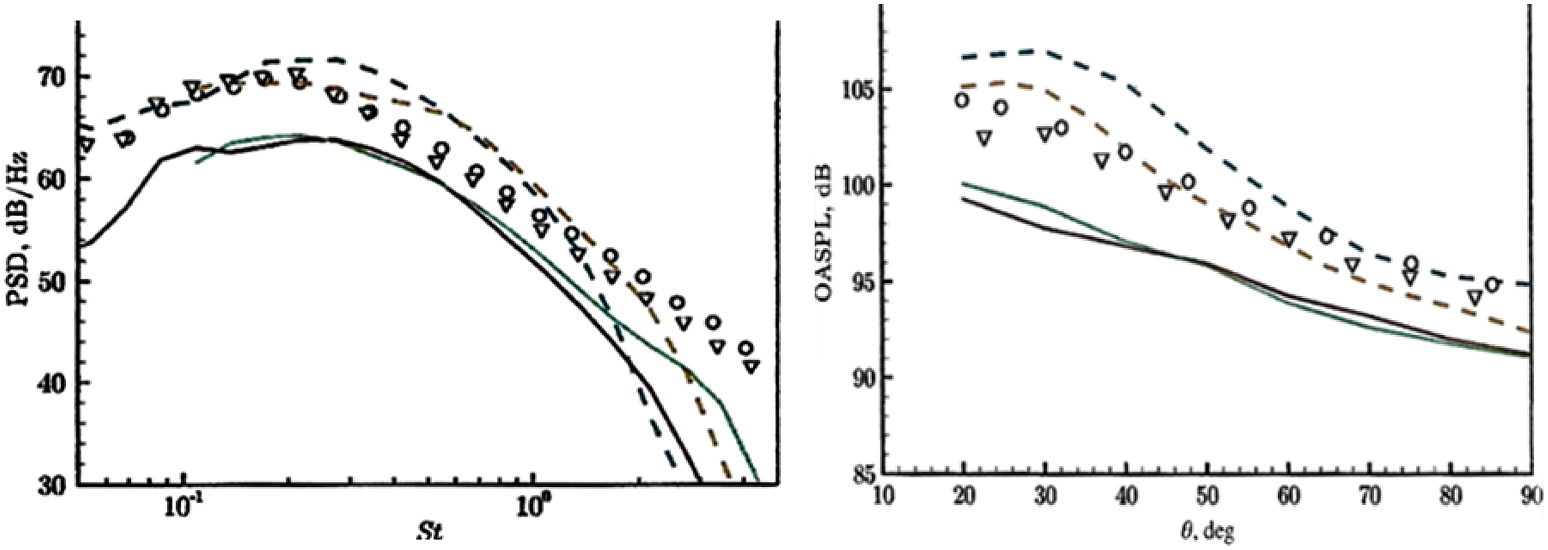
Figure 31. Left: LES/FWH (solid) and LES/APE (dashed) far-field PSD at
 $\theta\,=\,90^{\circ}$
with experiments from Refs Reference Brown and Bridges54, Reference Tanna17, from Ref. Reference Moratilla-Vega, Lackhove, Janicka, Xia and Page52. Right: LES/FWH (solid) and LES/APE (dashed) OASPL versus experiments of Refs Reference Brown and Bridges54, Reference Tanna17, from Ref. Reference Moratilla-Vega, Lackhove, Janicka, Xia and Page52.
$\theta\,=\,90^{\circ}$
with experiments from Refs Reference Brown and Bridges54, Reference Tanna17, from Ref. Reference Moratilla-Vega, Lackhove, Janicka, Xia and Page52. Right: LES/FWH (solid) and LES/APE (dashed) OASPL versus experiments of Refs Reference Brown and Bridges54, Reference Tanna17, from Ref. Reference Moratilla-Vega, Lackhove, Janicka, Xia and Page52.
3.2 Detailed consideration of nozzle effects
Arguments were put forward in Section 2, and by Brès et al. (Reference Brés, Jaunet, Le Rallic, Jordan, Colonius and Lele39,Reference Brés, Jordan, Jaunet, Le Rallic, Cavalieri, Towne, Lele, Colonius and Schmidt40), that for accurate simulation of high-frequency noise generated by the small-scale dynamically important eddies in the thin nozzle exit shear layer, it is important for exit boundary layer details to be accurately reproduced in the simulation. These have rarely been measured in experimental studies, and it is increasingly common for simulations to include internal nozzle flow. This is perhaps motivated by an assumption that detailed velocity/turbulence information is easier to obtain (or assumptions made in its estimation are less critical) at the nozzle inlet. This is certainly the case in laboratory/rig studies, and for realistic aeroengine geometries, CFD predictions of the flow upstream of the nozzle are now appearing (see below). To provide a test case for internal nozzle simulations, Trumper et al. (Reference Trumper, Behrouzi and McGuirk7) conducted an experimental study for a convergent nozzle with representative length/area change and at appropriate Re j and M j , providing the velocity and turbulence at the nozzle inlet and exit. Wang and McGuirk (Reference Wang and McGuirk55) reported LES for the same nozzle geometry, which is shown in Fig. 32 (top left).

Figure 32. Top: nozzle geometry (dimensions in mm) and instantaneous w-velocity contours. Bottom: LES mean axial velocity at nozzle exit, zoom-in for internal corner. From Ref. Reference Wang and McGuirk55.
The contracting area ratio is similar to that of the BAESystems Hawk aircraft. A small parallel extension at the nozzle exit was added to remove vena contracta effects and allow the thin, partially relaminarised, exit boundary layer to recover to the turbulent state expected of full-scale aeroengine conditions. The inlet measurements were used in the R2M LES inlet condition generation method of Ref. Reference Xiao, Dianat and McGuirk42 and captured measured inlet profiles very well (Fig. 22). An instantaneous snapshot of velocity contours from the simulation (Fig. 32, top right) illustrates the precursor (x/D up to 2.5) and main (2.5–4.17) LES domains. The w-component is plotted to illustrate the large-scale vortical structures in the boundary layer, angled away from the wall as observed in experiments; high acceleration within the nozzle stretches these longitudinally, reflecting experimental observations of increased streamwise integral scales in accelerated flows. The mean axial velocity field within the nozzle is shown in Fig. 32 (bottom left); the rapid acceleration reduces the boundary-layer thickness dramatically. The boundary layer begins to grow again in the short parallel extension: the
 $\delta_{99}$
layer thickness is 28% of the local diameter at the nozzle entry, 0.5% at the end of contraction and
$\delta_{99}$
layer thickness is 28% of the local diameter at the nozzle entry, 0.5% at the end of contraction and
 $\sim$
16% at the nozzle exit.
$\sim$
16% at the nozzle exit.
At the internal corner between convergence and parallel extension, flow turning creates a local region of acceleration/deceleration; the adverse pressure gradient is strong enough to cause a small separation region downstream of the corner, seen in the zoom-in displayed in Fig. 32 (bottom right) (note that this shows a small region only within 0.004D radially and 0.2D axially of the wall). However, the turbulence created by this separation clearly has an important effect on boundary-layer growth, affecting the near-wall velocity profile strongly. Figure 33 (left) compares LES and low-Re RANS model predictions of the internal nozzle flow, indicating the mean velocity profile at the nozzle outlet. This has been plotted in Clauser chart format to focus attention on the near-wall flow, where measurements are captured better by LES. This is also the case for nozzle exit turbulence conditions (Fig. 33 (right)), where the high axial turbulence rms measured near the nozzle lip is significantly underpredicted by RANS but reproduced well by LES. This investigation showed that nozzle exit conditions can be well represented by a careful simulation of the internal nozzle flow.
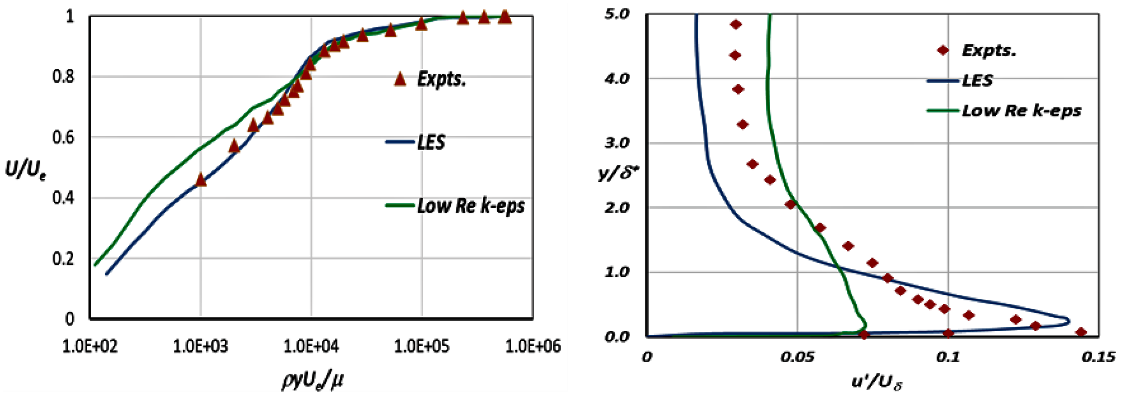
Figure 33. LES and low-Re RANS predicted exit axial velocity/turbulence rms versus experiments from Refs Reference Trumper, Behrouzi and McGuirk7, Reference Wang and McGuirk55.
The most comprehensive and ambitious LES of internal nozzle flow, also including jet near-field development and aeroacoustics, is that of Brès et al. (Reference Brés, Jordan, Jaunet, Le Rallic, Cavalieri, Towne, Lele, Colonius and Schmidt40,Reference Brés and Lele56). The computational set-up is presented in Fig. 34. The nozzle geometry was taken from a jet noise experiment conducted at Institut PPRIME in Poitiers (France) with NPR and NTR values of 1.7 and 1.15, respectively (M
j
= 0.9 and Re
j
= 106). The nozzle was a short (
 $\sim$
10D) straight pipe preceded by a contraction with area ratio of 7. Unfortunately, this is not representative of aeroengine nozzle shapes, omitting the relaminarising effect of an engine exhaust nozzle contraction geometry. In addition, to ensure a turbulent boundary layer at the nozzle exit, the transition was tripped by inclusion of a roughness strip
$\sim$
10D) straight pipe preceded by a contraction with area ratio of 7. Unfortunately, this is not representative of aeroengine nozzle shapes, omitting the relaminarising effect of an engine exhaust nozzle contraction geometry. In addition, to ensure a turbulent boundary layer at the nozzle exit, the transition was tripped by inclusion of a roughness strip
 $\sim$
2.5D upstream of the exit. The effects of this had to be modelled in the simulations (by adopting a form of the digital filter method41 and adjusting this until measurements made at x/D = 0.04 downstream of the nozzle exit were matched as far as possible). Wall-modelled LES was included following the approach proposed in Ref. Reference Kawai and Larsson34. A detailed study of mesh resolution and mesh design was also undertaken, and careful attention was paid to both inside the nozzle and in the jet region (details in Ref. Reference Brés, Jordan, Jaunet, Le Rallic, Cavalieri, Towne, Lele, Colonius and Schmidt40); the results shown below were obtained using 16 × 106 mesh points and an LES/FWH approach (with averaging of end caps) to propagate noise to the far field.
$\sim$
2.5D upstream of the exit. The effects of this had to be modelled in the simulations (by adopting a form of the digital filter method41 and adjusting this until measurements made at x/D = 0.04 downstream of the nozzle exit were matched as far as possible). Wall-modelled LES was included following the approach proposed in Ref. Reference Kawai and Larsson34. A detailed study of mesh resolution and mesh design was also undertaken, and careful attention was paid to both inside the nozzle and in the jet region (details in Ref. Reference Brés, Jordan, Jaunet, Le Rallic, Cavalieri, Towne, Lele, Colonius and Schmidt40); the results shown below were obtained using 16 × 106 mesh points and an LES/FWH approach (with averaging of end caps) to propagate noise to the far field.
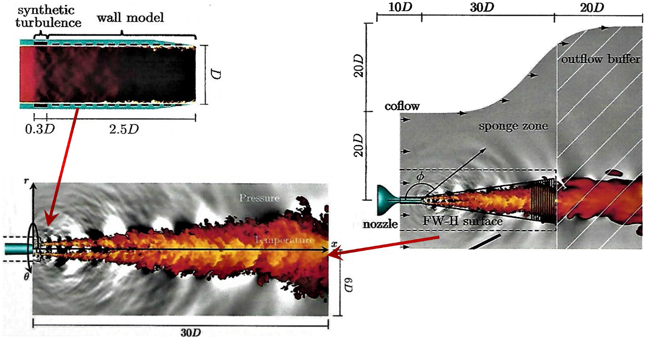
Figure 34. Simulation schematic: overall computational domain (top right), internal nozzle model (top left) and LES domain (bottom) from Ref. Reference Brés, Jordan, Jaunet, Le Rallic, Cavalieri, Towne, Lele, Colonius and Schmidt40.
The agreement with measurements for centreline and lipline axial mean and turbulence rms velocities is very good, as shown in Fig. 35 (top); the slight turbulence underprediction on the lipline is evidence that the nozzle exit conditions have not been perfectly reproduced by the internal nozzle modelling. Far-field acoustic predictions compared with measurements are shown in Fig. 35 (bottom) for the PSD at the 90° sideline angle and at four different values of M
j
(left) and an OASPL directivity distribution for M
j
=0.9 (right). The agreement is generally similar to that shown above for other isolated jet LES studies. The variation of the PSD with Mach number is reproduced well, with predicted spectra slightly closer to the data than shown above. As often observed with current LES, accuracy is very good up to St
 $\sim$
2 but deteriorates for higher frequencies, albeit lying above the data for this method rather than below as for the methods discussed above. Both of these features may be due to the measurements in Fig. 36 being made closer to the jet (radius
$\sim$
2 but deteriorates for higher frequencies, albeit lying above the data for this method rather than below as for the methods discussed above. Both of these features may be due to the measurements in Fig. 36 being made closer to the jet (radius
 $\sim$
15D) than for usual ‘far-field’ measurements (
$\sim$
15D) than for usual ‘far-field’ measurements (
 $\sim$
100D in Figs 29 and 31). All the results shown indicate that methods for considering nozzle exit profile details more than has traditionally been the case are now available.
$\sim$
100D in Figs 29 and 31). All the results shown indicate that methods for considering nozzle exit profile details more than has traditionally been the case are now available.
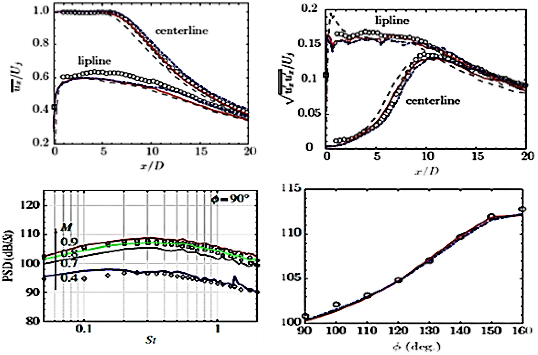
Figure 35. Top: LES predictions versus experiments for centreline and lipline. Bottom: LES/FWH versus experimental PSD (
 $\theta\,=\,90^{\circ}$
) for various M
j
, OASPL directivity M
j
= 0.9, from Refs Reference Brés, Jordan, Jaunet, Le Rallic, Cavalieri, Towne, Lele, Colonius and Schmidt40, Reference Brés and Lele56.
$\theta\,=\,90^{\circ}$
) for various M
j
, OASPL directivity M
j
= 0.9, from Refs Reference Brés, Jordan, Jaunet, Le Rallic, Cavalieri, Towne, Lele, Colonius and Schmidt40, Reference Brés and Lele56.
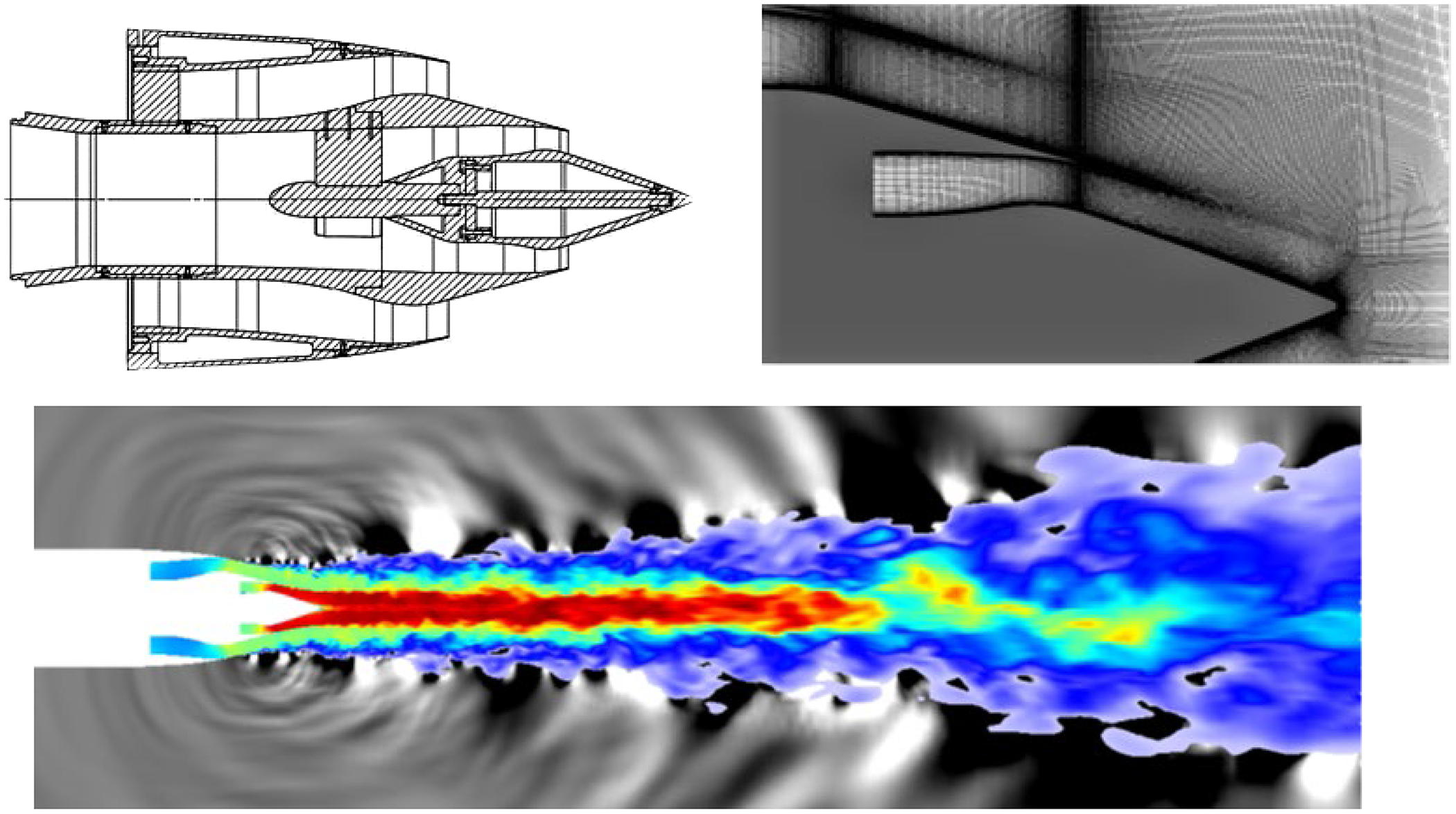
Figure 36. CoJeN short cowl co-axial nozzle showing geometry and near nozzle mesh (top) and instantaneous jet flow and near-field pressure waves (bottom), from Refs Reference Angelino, Xia and Page35, Reference Mead, Wrighton and Britchford57.
3.3 Co-axial nozzles
Modern aero-engines comprise dual rather than single stream jets, and extending the methods described above to co-axial nozzles is essential. The EU project Computation of Co-axial Jet Noise (CoJeN) provided an experimental database suitable for model evaluation (Reference Mead, Wrighton and Britchford57). The CoJen short cowl nozzle geometry is shown in Fig. 36 (top left); several operating points were explored, but case OP1.3 has usually been taken as the optimum validation case, since this includes the highest core and by-pass velocities as well as a heated core and produces the loudest noise signature. The core and by-pass velocities were U c, U bp = 480, 306m/s with a static temperature ratio of T s,c /Ts, bp = 2.7 (thus M c , Mbp = 0.88, 0.9), and no flight stream was present.
The LES/FWH method of Angelino et al. (Reference Angelino, Xia and Page35) has been applied to this case using a mesh of 80 × 106 cells. Figure 36 (top right) illustrates a zoom-in of the mesh in the nozzle vicinity, showing that a short length internal to both core and by-pass ducts has been included. Figure 36 (bottom) presents a snapshot of the near-field jet instantaneous flow field and pressure waves. A shielding effect of the by-pass jet can be seen, with entrainment into the core jet reducing and potential core length (red region) increasing. The pressure waves indicate sound sources located near the nozzle lips and at the potential core end, and a distinct direction of propagation at a low polar angle (
 $\theta$
=
$\theta$
=
 $\sim$
30°) as expected. The accuracy of the predicted velocity and turbulence fields is judged against PIV measurements for centreline development (Fig. 37, top). The initial centreline velocity is low due to the wake of the central plug, but rapidly accelerates up to the potential core end at
$\sim$
30°) as expected. The accuracy of the predicted velocity and turbulence fields is judged against PIV measurements for centreline development (Fig. 37, top). The initial centreline velocity is low due to the wake of the central plug, but rapidly accelerates up to the potential core end at
 $\sim$
x/D
bp. = 3.5; the subsequent rate of decay is well captured. The axial turbulence rms is also in good agreement with measured data, displaying a double peak with a maximum value slightly further downstream at
$\sim$
x/D
bp. = 3.5; the subsequent rate of decay is well captured. The axial turbulence rms is also in good agreement with measured data, displaying a double peak with a maximum value slightly further downstream at
 $\sim$
x/D
bp = 6.0. Acoustic results were azimuthally averaged, and Fig. 37 (bottom) shows the predicted PSD curves for two polar angles of
$\sim$
x/D
bp = 6.0. Acoustic results were azimuthally averaged, and Fig. 37 (bottom) shows the predicted PSD curves for two polar angles of
 $\theta\,=\,30^{\circ}$
(left) and
$\theta\,=\,30^{\circ}$
(left) and
 $\theta\,=\,120^{\circ}$
(right); agreement with experiments is good, the cut-off frequency for accuracy is St
$\theta\,=\,120^{\circ}$
(right); agreement with experiments is good, the cut-off frequency for accuracy is St
 $\sim$
3, but the peak noise level and decay rate as frequency increases are close to the data at both angles.
$\sim$
3, but the peak noise level and decay rate as frequency increases are close to the data at both angles.

Figure 37. LES/FWH versus experimental flow field (top) and acoustics (bottom) for short cowl nozzle from Refs Reference Angelino, Xia and Page35, Reference Markesteijn and Karabasov58.
These results imply that the quality of LES predictions seen in the single jet case is retained for co-axial jets. However, it is worthwhile to consider a second LES/FWH study of the CoJeN test case, by Markesteijn et al. (Reference Markesteijn and Karabasov58), whose method differs from others in two ways. Firstly, the numerical basis of the flow solver (the CABARET method) is fundamentally different, adopting a ‘compact formulation of a 2nd-order upwind leapfrog scheme’. A single-cell computational stencil is achieved by using separate conservation and flux variables staggered in space–time. The second difference is that advantage is taken of this asynchronous time stepping to decrease the computational cost via efficient parallel implementation of the algorithm on Graphics Processing Unit (GPU)-equipped workstations. The results are of similar quality as above, but the time to solution is claimed to be an order of magnitude shorter than for conventional LES. This approach has not been widely adopted to date, but since the long turn-round time of LES is a major disincentive for its further use in engineering design, it does appear worthy of wider exploitation. Figure 38 shows velocity and turbulence profiles reported in Ref. Reference Markesteijn and Karabasov58 for the CoJeN test case. The axial development shows little change between meshes of 50 and 82 × 106 cells, and the agreement with measured data is similar to that shown in Fig. 37. The far-field spectrum for
 $\theta\,=\,30^{\circ}$
in Fig. 38 (bottom left) is similar to that shown in Fig. 37. Finally, Ref. Reference Markesteijn and Karabasov58 provides an informative illustration of how an LES method could be used in design investigations. What is shown in Fig. 38 (bottom right) is the change in the OASL directivity curve as the operating point of the nozzle is altered. Thus, a change from OP1.3 to OP1.1 involves only a reduction of the core flow Mach number from M
c
= 0.88 to 0.62, and a change from OP1.2 to OP1.1 implies a change of M
c
from 0.74 to 0.62. Figure 38 plots the predicted versus measured Δ(OASPL) for the polar angle range from 30° to 120°, revealing accuracy within 1dB and good reproduction of the trend of measured data. This is a powerful demonstration of how LES could be used to inform designers of these trends rather than rig tests.
$\theta\,=\,30^{\circ}$
in Fig. 38 (bottom left) is similar to that shown in Fig. 37. Finally, Ref. Reference Markesteijn and Karabasov58 provides an informative illustration of how an LES method could be used in design investigations. What is shown in Fig. 38 (bottom right) is the change in the OASL directivity curve as the operating point of the nozzle is altered. Thus, a change from OP1.3 to OP1.1 involves only a reduction of the core flow Mach number from M
c
= 0.88 to 0.62, and a change from OP1.2 to OP1.1 implies a change of M
c
from 0.74 to 0.62. Figure 38 plots the predicted versus measured Δ(OASPL) for the polar angle range from 30° to 120°, revealing accuracy within 1dB and good reproduction of the trend of measured data. This is a powerful demonstration of how LES could be used to inform designers of these trends rather than rig tests.
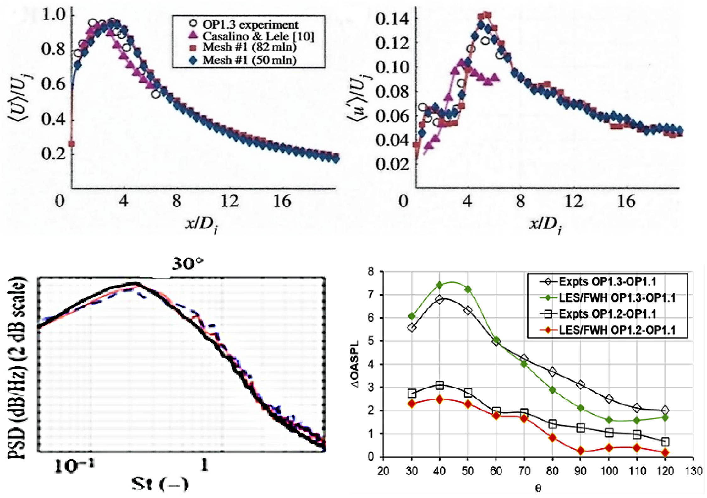
Figure 38. Short cowl nozzle: velocity (top), rms (middle) and acoustics (bottom) from Ref. Reference Markesteijn and Karabasov58.
3.4 Flight stream effects
Estimation of forward flight effects on jet noise is important since regulations on flyover noise are part of the certification process. Measurement using reduced-scale modes in wind tunnels has been the primary tool to quantify in-flight effects, although interference due to in-tunnel flow noise or refraction through the tunnel shear layer requires corrective measures. Viswanathan and Czech (Reference Viswanathan and Czech59) describe appropriate experimental/measurement techniques and the semi-empirical prediction models based on these, but a fundamentally based mathematical model capable of capturing in-flight effects would be valuable. The hybrid RANS/LES/FWH method of Ref. Reference Naqavi, Wang, Tucker, Mahak and Strange38 for an isolated jet described above has been extended to include flight effects by Wang et al. (Reference Wang, Naqavi, Tucker and Boehning60). Dominant noise sources are linked to shear-generated turbulence, and the principal effect of flight is to reduce shear; it is thus no surprise that flight effects lead to reduced noise. LES has a demonstrated capability to resolve turbulence-related noise sources, and this should transfer without any need for adaption to capture in-flight effects. The same is not the case for the FWH part of model, which as noted by Najafi-Yazdi et al. (Reference Najafi-Yazdi, Brés and Mongeau61) requires modification to a formulation based on the convective wave equation. Equally, the pseudo-sound generation caused by vortices moving through the FWH end-caps is exacerbated by a flight stream and needs special attention regarding the filtering method adopted (Reference Najafi-Yazdi, Brés and Mongeau61).
A selection of flow and acoustic predictions reported in Ref. Reference Wang, Naqavi, Tucker and Boehning60 are shown in Fig. 39 for a round nozzle hot jet with and without a flight stream: M j = 0.55, static temperature ratio = 2.7, Mfs = 0.3 and 0.0. Figure 39 (top) shows how the centreline and lipline axial velocity (left) and turbulent shear stress (right) change between static and flight stream conditions. The flight stream-reduced shear lowers entrainment, so the jet potential core length is almost doubled and the following velocity decay rate is also slower; the lipline velocity hardly changes over the axial distance covered. The peak Reynolds shear stress is reduced by 50%, and the peak axial stress on the centreline (Reference Wang, Naqavi, Tucker and Boehning60) is also 30% lower and shifted downstream. An overall impression of the acoustic field change is provided using the predicted sound wave patterns in Fig. 39 (middle). In the flight-stream case, a narrower and downstream-angled envelope is identifiable with increased higher-frequency waves at higher polar angles. The OASPL directivity curves shown in Fig. 39 (bottom) clearly illustrate the lower noise level, reduced by almost 10dB at the 30° polar angle and by 5dB in the upstream quadrant. Most importantly, the measured data are accurately reproduced by the LES/FHW approach, revealing that addition of a flight stream does not affected simulation performance.

Figure 39. Single jet without and with Mfs = 0.3 flight stream from Ref. Reference Wang, Naqavi, Tucker and Boehning60.
3.5 Design for noise reduction
The role played by shear-layer turbulence in controlling both noise source location and entrainment rate has encouraged designers to explore manipulation of jet mixing for noise reduction/control. Small ‘tabs’ attached to nozzle lips demonstrated increased mixing/reduced potential core length and were extensively researched in the 1980s and 1990s. The improved mixing was, however, accompanied by an increased level of total pressure loss that was unaffordable in the context of civil aircraft. This prompted industry/ National Aeronautics and Space Administration (NASA) to explore more subtle nozzle trailing-edge modifications including ‘chevrons’ or ‘serrations’, leading to substantial experimental programmes, and eventually technology introduction on aircraft in the early 2000s (Fig. 6). The review by Zaman et al. (Reference Zaman, Bridges and Huff62) describes the history of these developments. The experiments of Bridges and Brown (Reference Bridges and Brown63) represent a comprehensive examination of the influence of chevron geometry parameters, viz. count, radial penetration, axial length and azimuthal variations. Chevron count was found to be most influential, with high chevron count showing good low-frequency reduction without high-frequency penalty. Reductions of
 $\sim$
3EPNdB in take-off noise for
$\sim$
3EPNdB in take-off noise for
 $\sim$
0.5% cruise thrust loss were reported (Reference Saiyed, Mikkelsen and Bridges64).
$\sim$
0.5% cruise thrust loss were reported (Reference Saiyed, Mikkelsen and Bridges64).
Part of the experimental database that created the design understanding which underpinned the final technology has been adopted as a database to validate CFD capability for prediction of nozzle trailing-edge treatments for noise reduction. Several LES studies have focussed on chevron performance and used the experimental data of Bridges and Brown (Reference Bridges and Brown63) in which ten chevron geometries were tested and compared against data from a ‘clean’ datum nozzle. The test case favoured for LES validation is the serrated nozzle geometry SMC006 containing six symmetric chevrons, since this was the most effective for noise reduction. The SMC006 geometry is illustrated in Fig. 40 (top left), and the important chevron flow features predicted by LES are shown in Fig. 40 (top right). The streamwise vorticity created by each chevron acts to increase mixing via two mechanisms: an increased turbulence level close to the nozzle exit beneficially changing the downstream large-scale eddies that create low-frequency noise (although also causing high-frequency noise uplift) and an enlarged interfacial mixing interface between jet and ambient fluid. Figure 40 is taken from the LES study of Uzun and Hussaini (Reference Uzun and Hussaini65); this focussed attention on the near-nozzle, high-frequency noise-generating region and used a very fine mesh of 400 × 106 cells. However, this also clearly illustrated the conflict of exceedingly high mesh size as the high frequencies were captured, but the simulation duration was inadequate to allow statistically meaningful resolution of low-frequency sound. Results from three selected CFD studies of the SMC006 flow are included here: The first, by Xia and Tucker (Reference Xia and Tucker66), represents the hybrid RANS/LES/FWH method, while the second, by Angelino et al. (Reference Angelino, Xia and Page53), applies the wall-modelled LES/FWH method. The third, by Depuru Mohan et al. (Reference Depuru Mohan, Dowling, Karabasov, Xia, Graham, Hynes and Tucker67), is included since it illustrates how the ‘LES-informed’ RANS approach described above for a round jet in Ref. Reference Karabasov, Afsar, Hynes, Dowling, McMullan, Pokora, Page and McGuirk46 may be re-calibrated using LES input from a chevron nozzle simulation.
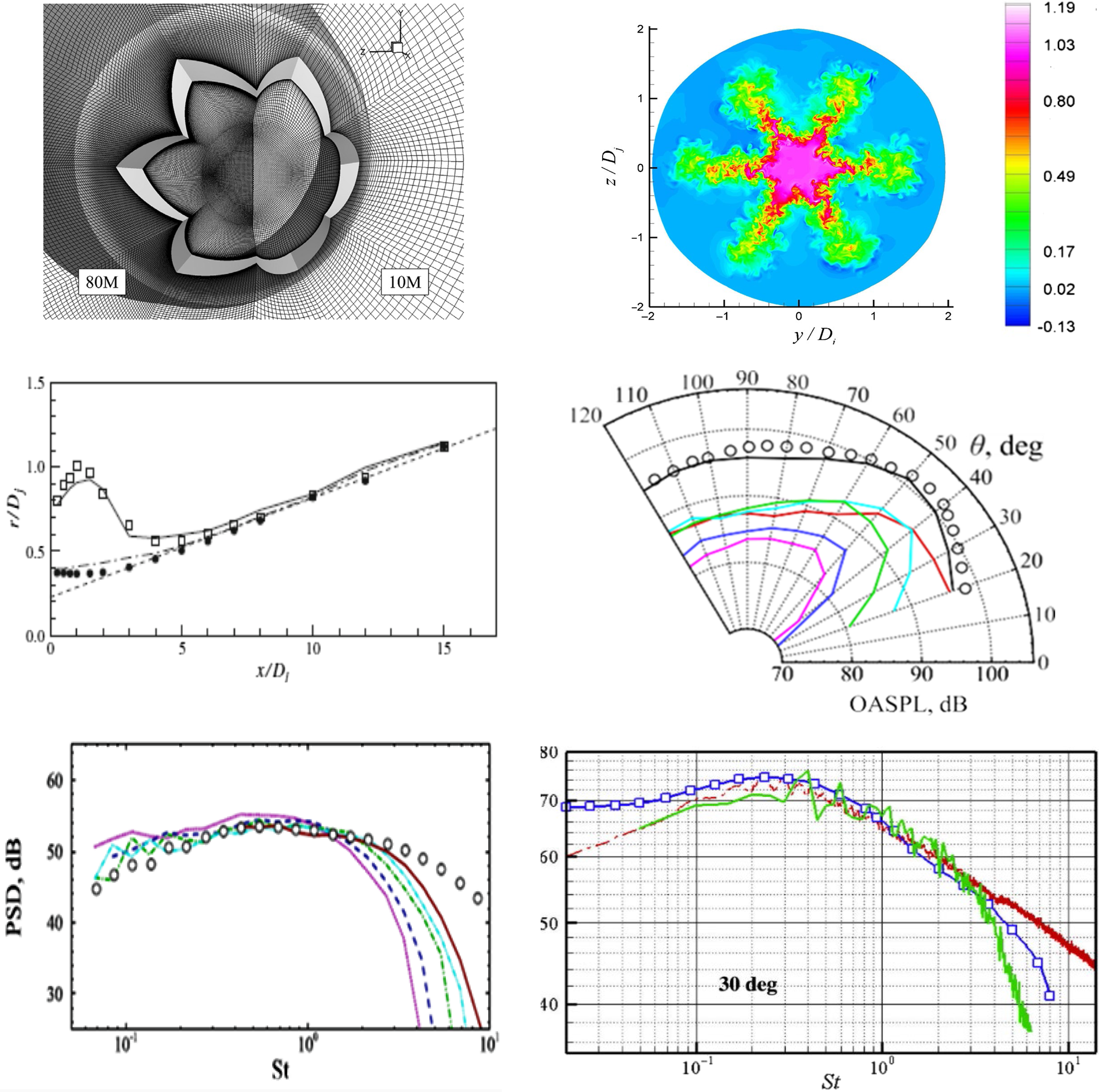
Figure 40. Top: nozzle geometry and mesh and instantaneous contours at x/D = 2 from Ref. Reference Angelino, Xia and Page53, Reference Uzun and Hussaini65. Middle: predicted jet spread and OASPL with azimuthal mode breakdown from Refs Reference Xia and Tucker66, Reference Angelino, Xia and Page53. Bottom: predicted far-field sound PSD at 90° and 30° from Refs Reference Angelino, Xia and Page53, Reference Depuru Mohan, Dowling, Karabasov, Xia, Graham, Hynes and Tucker67.
As for the simple round jet, the performance of hybrid and full LES methods is broadly similar for chevron nozzle flow, with the higher mesh levels of the full LES results showing a small improvement in accuracy at higher Strouhal number. The jet flow is deflected inwards at chevron tips and spreads outward in chevron troughs. Measurements of this aspect are well predicted, as seen in Fig. 40 (middle left). The ‘mild’ chevron radial penetration is indicated by a return to axisymmetric spreading after just 6D
j
. A reduced OASPL signature of
 $\sim$
2dB at low polar angles with the chevron nozzle may be seen by comparing Fig. 40 (middle left) with Fig. 29 (right). Finally, Fig. 40 (bottom right) compares a measured PSD at 30° for the chevron nozzle (red line) with predictions from the hybrid RANS/LES solution of Ref. Reference Xia and Tucker66 (green line) and the LES-informed RANS model of Ref. Reference Depuru Mohan, Dowling, Karabasov, Xia, Graham, Hynes and Tucker67 (blue line). In this latter, following the route proposed in Ref. Reference Karabasov, Afsar, Hynes, Dowling, McMullan, Pokora, Page and McGuirk46, the calibration constants used to scale turbulent velocity/length/time scales in the acoustic model have been re-calibrated using an LES chevron simulation and extended to include anisotropic length scales. Although this low-order model overpredicts the low-frequency part of the spectrum, it provides results closer to measurements at the higher frequencies that are difficult for LES/FWH. This perhaps implies that the acoustic propagation approach of Refs Reference Karabasov, Afsar, Hynes, Dowling, McMullan, Pokora, Page and McGuirk46 and Reference Depuru Mohan, Dowling, Karabasov, Xia, Graham, Hynes and Tucker67 could also be of some benefit for improving the propagation component of LES predictions.
$\sim$
2dB at low polar angles with the chevron nozzle may be seen by comparing Fig. 40 (middle left) with Fig. 29 (right). Finally, Fig. 40 (bottom right) compares a measured PSD at 30° for the chevron nozzle (red line) with predictions from the hybrid RANS/LES solution of Ref. Reference Xia and Tucker66 (green line) and the LES-informed RANS model of Ref. Reference Depuru Mohan, Dowling, Karabasov, Xia, Graham, Hynes and Tucker67 (blue line). In this latter, following the route proposed in Ref. Reference Karabasov, Afsar, Hynes, Dowling, McMullan, Pokora, Page and McGuirk46, the calibration constants used to scale turbulent velocity/length/time scales in the acoustic model have been re-calibrated using an LES chevron simulation and extended to include anisotropic length scales. Although this low-order model overpredicts the low-frequency part of the spectrum, it provides results closer to measurements at the higher frequencies that are difficult for LES/FWH. This perhaps implies that the acoustic propagation approach of Refs Reference Karabasov, Afsar, Hynes, Dowling, McMullan, Pokora, Page and McGuirk46 and Reference Depuru Mohan, Dowling, Karabasov, Xia, Graham, Hynes and Tucker67 could also be of some benefit for improving the propagation component of LES predictions.
3.6 Installation effects
Examples thus far have considered only the nozzle component of the engine geometry. Influence on the jet plume from other parts of the engine and the aircraft itself can also impact on flow development and aeroacoustics. This has become even more relevant since, motivated by lower fuel burn, the trend in engine design is for larger by-pass ratio. Indeed, ultra-high bypass ratios of 15–20 have been proposed. Increasing the engine diameter inevitably strengthens the interaction between the jet plume and wing/flaps, particularly when high-lift systems are deployed. The aerodynamic and aeroacoustic consequences that result are often described as ‘installation effects’. Semi-analytic models (Reference Lyu, Dowling and Naqavi68) with input from LES to calibrate correlation functions as described in Subsection 2.2 (Reference Karabasov, Afsar, Hynes, Dowling, McMullan, Pokora, Page and McGuirk46) as well as experimental studies (Reference Jordan, Jaunet, Towne, Cavalieri, Colonius, Schmidt and Agarwal69) have been carried out on a simplified installed jet geometry: a jet discharged close to a flat plate, as shown in Fig. 41 (top left), identifying extra noise sources due to scattering of near-field hydrodynamic pressure waves from the plate trailing edge, tonal components when the jet flow grazes the plate edge and surface reflection and jet flow-field refraction effects. The hybrid RANS/LES/FWH technique has recently been applied to this basic test problem by Wang et al. (Reference Wang, Proenca, Lawrence, Tucker and Self70) and compared with experimental measurements for M j = 0.6, H/D = 1 and L/D = 4 for both an isolated and an installed jet (using a mesh density of 50 × 106 cells for the installed case). Good agreement with mean velocity and turbulence profiles was demonstrated up to x/D = 10. For an isolated jet, the near-field hydrodynamic pressure fluctuations were also examined, producing the interesting plot shown in Fig. 41 (top right) for two radial positions at x/D = 2. Close to the jet at r/D = 1, the hydrodynamic contribution is identified by the hump at low frequency, whereas the fluctuations for St > 1 correspond to the acoustic contribution; further away at r/D = 2, the amplitude of the evanescent hydrodynamic part has decayed exponentially but the acoustic component remains, decaying with 1/r 2. Note that the LES results when compared directly with the measured near-field spectra reproduce these accurately, implying that fluctuating pressure noise sources are well resolved by LES.
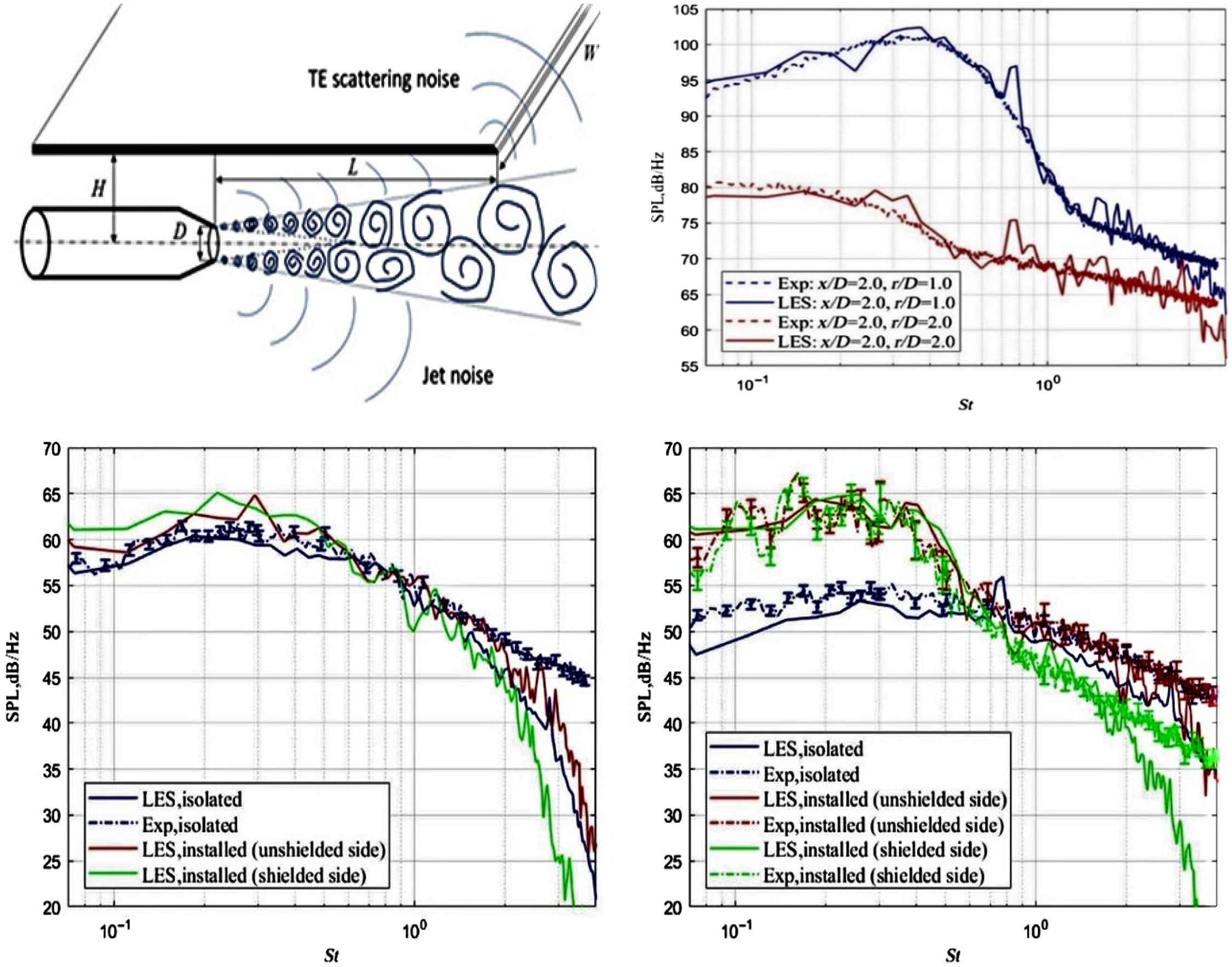
Figure 41. Jet discharged near a flat plate: near-field and far-field pressure PSD from Ref Reference Wang, Proenca, Lawrence, Tucker and Self70.
To compare with the measured far-field noise PSD, the FWH predictions are shown for both isolated and installed jets in Fig. 41 (bottom) for observer polar angles of 40° (left) and 90° (right). At 40° there is little difference in the predicted PSD curves between the installed (lower) and shielded (upper) sides of the plate, and simulations with and without the plate are close to the measured isolated jet PSD (except again for the too rapid fall-off for St >
 $\sim$
2 that continues to appear in all LES/FWH results). At 90°, however, installation effects are more noticeable and are again well captured by the simulations. For St < 0.5, large (10dB) noise uplift is observed, relative to the isolated jet, a consequence of jet–surface interaction. At higher frequencies, noise is reduced by shielding above the plate but increased by reflection below the plate. The ability of the LES/FWH approach to capture these installation effects is very encouraging.
$\sim$
2 that continues to appear in all LES/FWH results). At 90°, however, installation effects are more noticeable and are again well captured by the simulations. For St < 0.5, large (10dB) noise uplift is observed, relative to the isolated jet, a consequence of jet–surface interaction. At higher frequencies, noise is reduced by shielding above the plate but increased by reflection below the plate. The ability of the LES/FWH approach to capture these installation effects is very encouraging.
In engineering applications, the geometry of near-nozzle/jet surfaces is considerably more complex and includes lifting surfaces. Scenarios involving more complex and realistic geometries have been considered using the full LES approach in Ref. Reference Angelino, Moratilla-Vega, Howlett, Xia and Page5 and, to a greater extent, the hybrid RANS/LES/FWH technique in Refs Reference Tyacke, Mahak and Tucker71–Reference Tyacke, Wang and Tucker74.
The flow configuration used by Angelino et al. (Reference Angelino, Moratilla-Vega, Howlett, Xia and Page5) specifically focussed on possible interference of high flap deflection angles on jet plume development. The geometry and experimental data were taken from the Innovate UK SYMPHONY project and comprised a simplified transport aircraft fuselage, one wing with flaps deployed (at two angles of 16° and 32°) and a coaxial engine nozzle plus pylon. Flow conditions were representative of post-take-off flight, and a mesh of 120 × 106 cells was used. Figure 42 (top left) shows an instantaneous picture of the jet flow and the acoustic field on a cut plane immediately below the engine for the higher flap angle, for which stronger interaction and deflection of the jet plume were observed, as seen in the instantaneous velocity contour plot in Fig. 42 (top right).
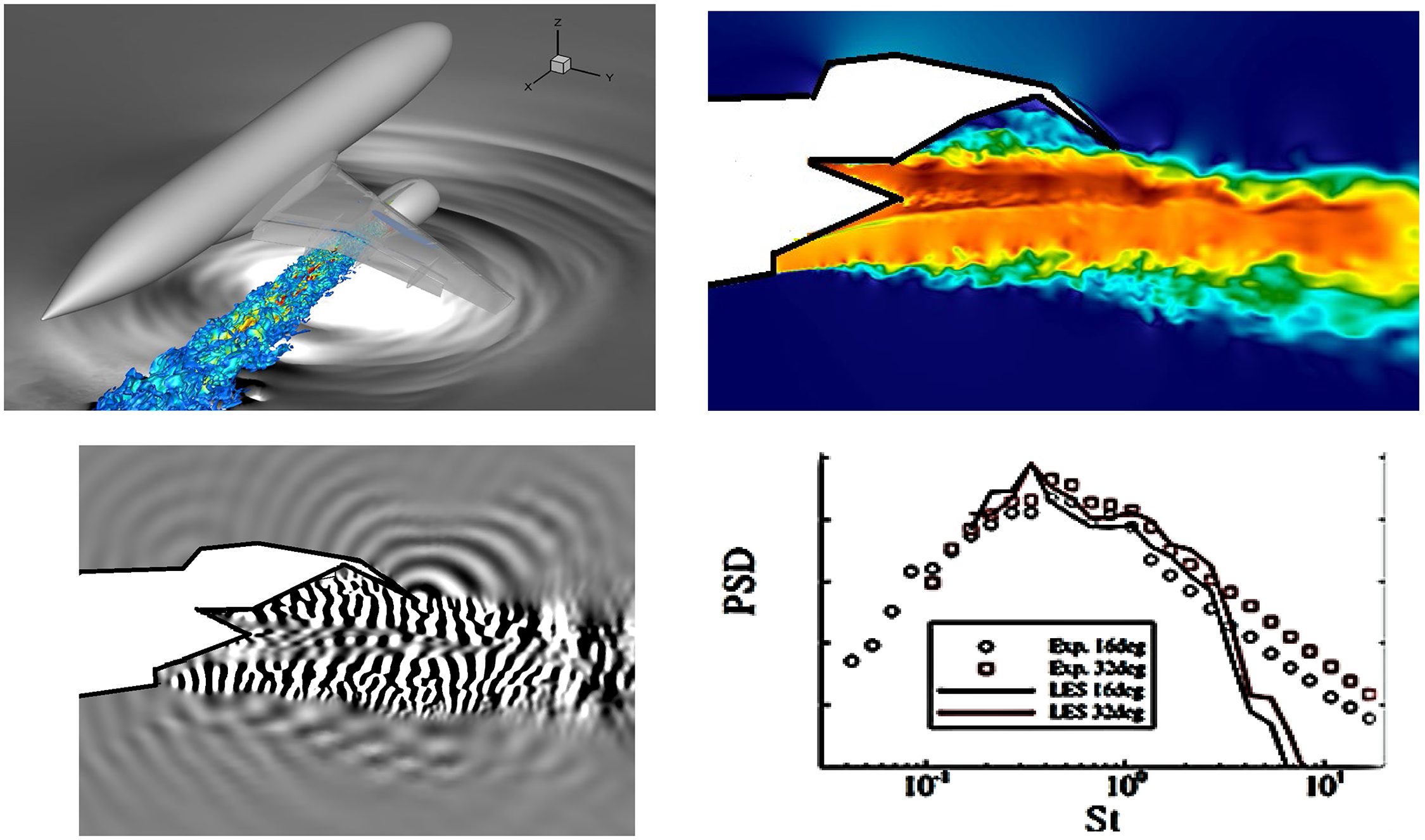
Figure 42. Installation noise simulation: flow field, near-field acoustics and far-field PSD from Ref Reference Angelino, Moratilla-Vega, Howlett, Xia and Page5.
To quantify the consequences of wing flap–jet interaction, the pressure field was Fourier-analysed and filtered at specific Strouhal numbers; the real part of the transform at St = 1.0 is displayed in Fig. 42 (bottom left), revealing a dominant noise source at the flap trailing edge as well as waves associated with scattering from the wing leading edge and the jet near field. The far-field PSD obtained using the LES/FWH approach at the forward observer polar angle of 120° is compared with measured data in Fig. 42 (bottom right). The usual degradation at high frequency is seen, but both experiments and simulations indicate a shift in noise level due to the two different flap angles of
 $\sim$
3dB.
$\sim$
3dB.
In a series of papers, Tyacke, Wang and Tucker (Reference Tyacke, Mahak and Tucker71–Reference Tyacke, Wang and Tucker74) modified and extended their hybrid RANS/LES/FWH approach to increasingly more complex geometries. The method has been demonstrated to capture installation effects which include a wing with deflected flaps, an engine nacelle with pylon, a serrated nozzle, a flight stream and even a treatment considering the airflow through the fan, Outlet Guide Vane (OGV) and by-pass duct to set inlet conditions at entry to the by-pass nozzle as closely as possible to those occurring in practice. Two examples are selected here to indicate the significant progress made. The first, reported in Refs Reference Tyacke, Wang and Tucker72–Reference Tyacke, Wang and Tucker74, describes the capability for analysis of a combination of chevrons, wing/flap interference and a flight stream; the second (Reference Tyacke, Mahak and Tucker71) illustrates how inlet conditions for the by-pass nozzle can take into account effects of upstream turbomachinery and engine component blockages.
Figure 43 (top left) indicates the first scenario, showing a vertical cross-section through the engine axis. In this simulation, nozzle inlet conditions for both by-pass and core are specified total pressure, temperature and mass flow, with the flight stream set at 90m/s. The red lines indicate regions close to walls where RANS modelling was applied, with an LES mesh of 120–150 × 106 cells depending on the precise geometry included. The combined complexity of twin jet streams, nacelle (pylon not included at his stage) and wing/deployed flap (flap angles of 8° and 14° investigated) requires considerable effort to design and create a well-designed mesh (refined in all critical regions). Several blocks of mesh are needed (hexahedral to ensure accurate resolution of shear layers), with the more dissipative unstructured mesh restricted to regions removed from high gradient, high turbulence zones; prism layers are necessary to interface between hexahedral and unstructured regions, creating the complex grid topology illustrated in Fig. 43 (top right). If a serrated nozzle is included, it was found necessary to introduce distortions in the hexahedral mesh zones covering the initial jet region to improve accuracy in the convoluted shear layers created by chevrons. Portions of the hexahedral mesh were shifted to fit a ‘shear-layer location’ line in space, defined using an a priori RANS calculation of the serrated nozzle. The geometry of the 16 serrations at the nozzle exit is shown in Fig. 43 (bottom left) together with the RANS solution used to guide mesh distortion. The resulting mesh and a snapshot of the LES solution just downstream of the serrated nozzle trailing edge are shown in Fig. 43 (bottom right).
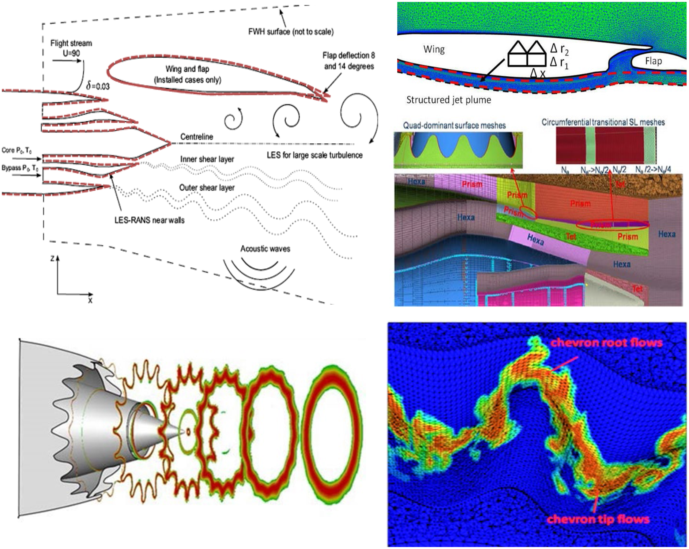
Figure 43. Zonal modelling and meshing approach, RANS solution and chevron mesh from Refs Reference Tyacke, Wang and Tucker72, Reference Tyacke, Wang and Tucker73.
In the case considered in Refs Reference Tyacke, Wang and Tucker73–Reference Brés, Ham, Nichols and Lele75, NPR values in core and by-pass were low (
 $\sim$
1.28) and, with a 90m/s flight stream, velocity ratios across the shear layers were low, leading to low levels of turbulence energy, higher in the by-pass/ambient shear layer, as shown in Fig. 44 (top left). For the larger (14°) flap deflection, the shear layer–flap interaction is obviously greater than at 8°, generating higher turbulence and displaying a flap-induced deflection of the outer shear layer, which spreads faster than the shear layer on the ground side, reaching the engine axis at
$\sim$
1.28) and, with a 90m/s flight stream, velocity ratios across the shear layers were low, leading to low levels of turbulence energy, higher in the by-pass/ambient shear layer, as shown in Fig. 44 (top left). For the larger (14°) flap deflection, the shear layer–flap interaction is obviously greater than at 8°, generating higher turbulence and displaying a flap-induced deflection of the outer shear layer, which spreads faster than the shear layer on the ground side, reaching the engine axis at
 $\sim$
x/D = 10. The influence of the wing-side shear layer flow on the flow within and through the wing/flap recess is displayed in Fig. 44 (top right); the turbulence intensity inside the recess increases to
$\sim$
x/D = 10. The influence of the wing-side shear layer flow on the flow within and through the wing/flap recess is displayed in Fig. 44 (top right); the turbulence intensity inside the recess increases to
 $\sim$
50% near the wing trailing edge and is also high on the leading-edge underside of the flap, creating a new noise source. The influence of the jet plume on wing aerodynamics can now also be assessed, and this is visible in the contour map of the static pressure coefficient on the lower wing surface shown in Fig. 44 (middle left). The small red region is absent for no flap deflection, just visible for 8° and has grown and intensified considerably at 14°; fluctuating pressure data are also provided in Ref. Reference Brés, Ham, Nichols and Lele75, which is valuable information for potential structural fatigue analysis.
$\sim$
50% near the wing trailing edge and is also high on the leading-edge underside of the flap, creating a new noise source. The influence of the jet plume on wing aerodynamics can now also be assessed, and this is visible in the contour map of the static pressure coefficient on the lower wing surface shown in Fig. 44 (middle left). The small red region is absent for no flap deflection, just visible for 8° and has grown and intensified considerably at 14°; fluctuating pressure data are also provided in Ref. Reference Brés, Ham, Nichols and Lele75, which is valuable information for potential structural fatigue analysis.
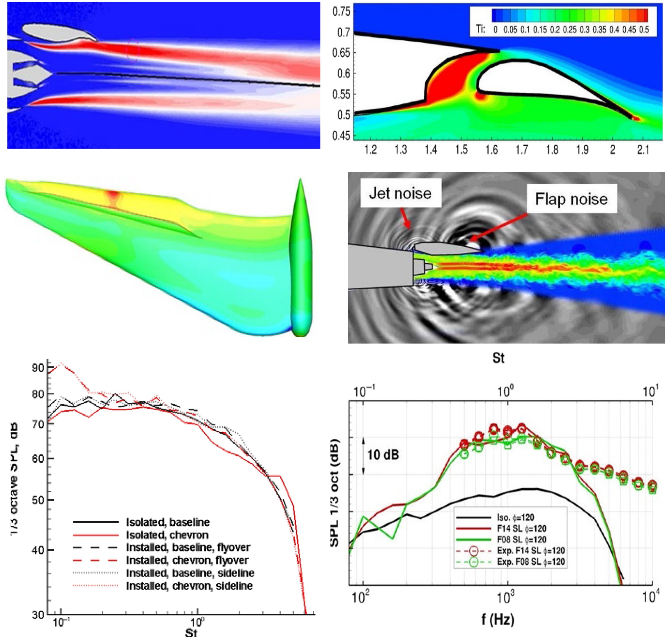
Figure 44. LES/FWH analysis of chevron nozzle/wing/flap installation noise from Ref. Reference Tyacke, Wang and Tucker73, Reference Tyacke, Wang and Tucker74.
Figure 44 (middle right and bottom) shows three results from the acoustic predictions. The first presents an instantaneous snapshot of pressure fluctuation waves, providing indications of the noise sources. The expected propagation pattern of jet noise is revealed, but indications of a noise source located near the flap are also seen, as is a high-frequency source from the wing leading edge, cause by scattering of jet noise waves. Far-field PSD plots are given in Fig. 44 (bottom); on the left are shown curves for a 120° polar angle with isolated and installed jet plumes from round (baseline) and chevron nozzles. The addition of chevrons reduces the low-frequency noise but shows a notable uplift at high frequency; installation effects significantly increase noise due to wing and jet/flap interactions. There are no experimental data to confirm these results quantitatively, but for the slender wing/round nozzle case considered in Ref. Reference Tyacke, Wang and Tucker74, Fig. 44 (bottom right) provides a PSD plot for f = 120° which confirms that the simulation has captured the installation effects compared with an isolated case very well. The slight increase as the flap angle increases near St =1.0 as seen in measurements is also reproduced, again a very encouraging result.
Finally, the emphasis in the work reported in Ref. Reference Tyacke, Mahak and Tucker71 was to explore improved specification of by-pass nozzle inlet conditions by including the effect of upstream internal engine flow. The engine geometry (Fig. 45 (top left)) was created by adding an axisymmetric inlet, hub and splitter geometry to the nozzle and rear engine shape that was already defined in the CoJeN project (Fig. 36). In addition, a ‘RANS-type’ approach was introduced for the annular duct supplying the by-pass nozzle, to include (at least partially) effects of turbomachinery and large-scale blockages. On computational cost grounds, the by-pass flow prediction was not a genuine geometry-resolving RANS solution. Rather, the fan, OGVs and large components in the duct expected to create significant wakes (engine A-frame and gearbox shaft) were introduced into an axisymmetric by-pass duct using body forces. The resulting methodology was labelled ‘multi-fidelity, multi-physics’ since it involves: (i) an approximate (‘smeared’ due to the body force model) RANS solution for the by-pass flow, (ii) a full RANS solution for both the core nozzle flow from the CoJeN nozzle inlet plane and including trailing-edge serrations) as well as in general all near-wall flows and (iii) an LES of the jet and induced flow external to the engine. The core nozzle inlet specification was retained as fixed total pressure/temperature/mass flow.
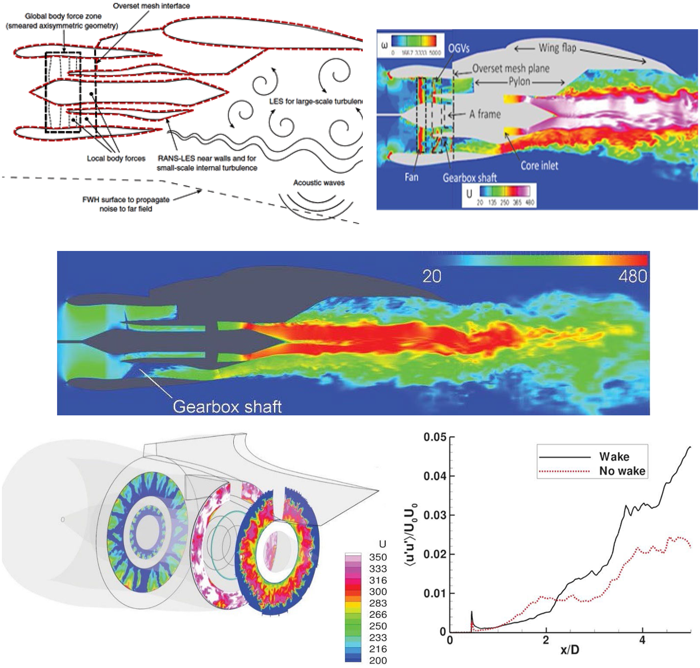
Figure 45. Simulation accounting for engine effects in by-pass stream from Ref. Reference Tyacke, Mahak and Tucker71.
Figure 45 shows the various geometry components included (left) and an instantaneous snapshot (right) of vorticity created by the internal body forces and of axial velocity in the jet plume, providing an overall impression of the flow field. Axial velocity contours on a vertical cross-section through the engine mid-plane in Fig. 45 (middle) provide a picture of the development of the velocity field through the engine in the by-pass duct. The fan location may be identified by the green/blue contour colour change in the front of the engine, and the gearbox shaft obstruction is seen in the lower by-pass duct. Figure 45 (bottom) presents three axial planes showing contours of instantaneous axial velocity (all lying within the LES domain): (i) at the rear of the by-pass duct aft of internal geometry, (ii) at the by-pass duct exit and (iii) halfway along the pylon. Multiple wakes due to fan OGVs are present at the first plane, the flow accelerates up to the second plane, reducing in-plane velocity variation but these remain significant, and a complex pattern is still present at the third plane. The implication is that a spatially varying pattern of velocity/turbulence persists up to the by-pass nozzle inlet and may need to be considered to capture plume near-field development accurately.
The part of the jet plume most affected by inclusion of upstream engine effects into the by-pass nozzle inlet conditions is the by-pass/ambient shear layer, in which turbulence is generated more rapidly than in the by-pass/core shear layer. The different turbulence field emerging from the by-pass nozzle when upstream effects are included compared with an estimated nozzle condition may be significant but in the presence of a flight stream would reduce this effect. No acoustics calculations were carried out in this study, and the significance of these arguments remains to be confirmed. However, Fig. 45 (bottom right) indicates how the axial turbulence along the lipline between the core nozzle and by-pass stream reacts when the by-pass nozzle inlet conditions are changed from fixed (no wakes) to that produced by body force-driven RANS solution with wakes: substantial differences are seen.
These results illustrate an important point: this is the first calculation where nozzle inlet profiles have been generated using calculated details of the upstream flow, including turbomachinery effects. The body force technique embedded in a RANS solution may not deliver the precise mean velocity and turbulence profiles leaving the by-pass system and entering the nozzle, but it is a large step in the right direction. It would certainly be of interest to explore using the body force approach in an LES prediction of the by-pass duct as well as the core flow duct aft of the Low-Pressure (LP) turbine, to deliver the best possible estimate of nozzle exit conditions (including turbulence) for jet plume prediction. The acoustic consequences of introducing these effects also need to be explored, and validation measurements made to establish the adequacy of the body force approach.
4.0 Military aerospace applications
4.1 Supersonic jets from isolated nozzles
Extension of the LES/FWH approach to supersonic jets, including imperfect expansion, has been described by Brès et al. (Reference Brés, Ham, Nichols and Lele75) for a round con-di nozzle (on-design NPR = 3.67 and M j = 1.5) operated over-expanded at NPR = 2.97 and M j = 1.35 (fully expanded), with a heated jet NTR = 2.53 (T j /T amb = 1.85). The same LES/FWH numerical techniques were applied as in the subsonic simulations of Ref. Reference Klein, Sadiki and Janicka41 with added treatment to improve shock capturing.
The mesh used consisted of 55 × 106 cells, with a mesh strategy applied to ensure cell aspect ratios close to unity within the main noise source region as avoiding too rapid grid stretching was observed to reduce overprediction of high-frequency noise at upstream radiation angles. Figure 46 (top) provides a global view of the simulation with instantaneous temperature contours within the jet plume and pressure waves outside. The Mach wave radiation pattern excited by the motion of large-scale turbulent eddies produces a dominant propagation angle of
 $\phi\;\sim$
30–40°; the origin of noise sources creating spherical waves occurs at the potential core end. The temperature contours indicate the over/under-expansion behaviour in the early part of the jet. Predicted flow statistics for axial velocity along centreline and nozzle lipline are given in Fig. 46 (middle); measurements are only available for a perfectly expanded heated jet case, but these show similar characteristics as in subsonic LES jets with accurate capture of the potential core length and good agreement with the downstream velocity decay rate. The imperfectly expanded condition produces ten shock cell oscillations, with weak oscillations also observed on the lipline. Finally, Fig. 46 (bottom) compares the predicted PSD spectra at
$\phi\;\sim$
30–40°; the origin of noise sources creating spherical waves occurs at the potential core end. The temperature contours indicate the over/under-expansion behaviour in the early part of the jet. Predicted flow statistics for axial velocity along centreline and nozzle lipline are given in Fig. 46 (middle); measurements are only available for a perfectly expanded heated jet case, but these show similar characteristics as in subsonic LES jets with accurate capture of the potential core length and good agreement with the downstream velocity decay rate. The imperfectly expanded condition produces ten shock cell oscillations, with weak oscillations also observed on the lipline. Finally, Fig. 46 (bottom) compares the predicted PSD spectra at
 $\phi$
= 90° for both perfectly and over-expanded jets plotted against St. The agreement is good apart from slight underprediction of noise amplitude at low frequencies, explained in Ref. Reference Wang and McGuirk76 as caused by insufficient temporal sampling in the simulation, a problem already identified in subsonic LES with very fine meshes. Most importantly, the change in shape brought about by the onset of broadband shock noise in the over-expanded case (the ‘hump’ at St
$\phi$
= 90° for both perfectly and over-expanded jets plotted against St. The agreement is good apart from slight underprediction of noise amplitude at low frequencies, explained in Ref. Reference Wang and McGuirk76 as caused by insufficient temporal sampling in the simulation, a problem already identified in subsonic LES with very fine meshes. Most importantly, the change in shape brought about by the onset of broadband shock noise in the over-expanded case (the ‘hump’ at St
 $\sim$
0.9 and
$\sim$
0.9 and
 $\phi$
= 90°) is reproduced accurately.
$\phi$
= 90°) is reproduced accurately.

Figure 46. Overexpanded round jet, flow field, mean axial velocity and far-field PSD at 90° from Ref. Reference Brés, Ham, Nichols and Lele75.
Whilst this good agreement for round supersonic jets is the first stage of demonstrating good LES performance, high-aspect-ratio (AR) rectangular letterbox-shaped nozzles are more favoured in military applications due to the ease with which they can be integrated into the airframe and the higher mixing rate they provide; validation against such nozzle geometries is thus essential. The capability of LES to address the aerodynamic aspects of military-style nozzles was investigated in a combined experimental/LES study by Wang and McGuirk (Reference Wang and McGuirk76), focussed particularly on validating the accuracy of the potential core length and initial decay rate prediction, as these are so crucial for the IR signature. A recent study by Chakrabarti et al. (Reference Chakrabarti, Unnikrishnan, Gaitonde, Stack, Baier, Karnam and Gutmark77) reports a similar measurements/LES study, although for a low-aspect-ratio nozzle (AR = 2). Particular attention was paid to the over-expanded NPR hot jet condition which is relevant to take-off when acoustic signature constitutes a significant problem. The problem of nozzle internal shock systems caused by non-contoured (straight line) con-di geometries (typical in practice) and imperfectly expanded jets was also examined thoroughly in Ref. Reference Chakrabarti, Unnikrishnan, Gaitonde, Stack, Baier, Karnam and Gutmark77.
The AR = 4 con-di nozzle used in Ref. Reference Wang and McGuirk76 is shown in Fig. 47 (top left); Laser Doppler Anemometry (LDA) measurements were carried out in the major and minor axis planes within the jet plume near field, but also at an upstream nozzle inlet plane (through optical windows in the sidewalls, Fig. 47 (top right)) to provide guidance on inlet profiles. The nozzle design NPR was 4 with properly expanded exit Mach and Reynolds numbers of 1.58 and 1.7 × 10⁶, respectively. Detailed measurements were made under cold conditions (NTR = 1.0) for an over-expanded NPR of 2.5 to ensure the presence of significant shock and expansion waves. The mesh of 30 × 106 cells with extra refinement placed carefully in boundary layer, shear layer and expected shock locations was found to be adequate; measured inlet conditions were generated by the R2M inlet condition technique (Reference Xiao, Dianat and McGuirk42). Two LES sub-grid-scale (SGS) models were compared.
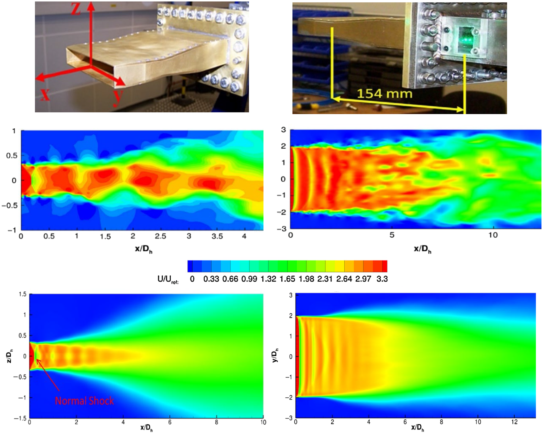
Figure 47. Rectangular nozzle: instantaneous and time-mean axial velocity contours from Ref. Reference Wang and McGuirk76.
Instantaneous and time-mean contours of axial velocity on minor (left) and major (right) axis planes from the simulation are shown in Fig. 47 (middle and bottom). The plume shear layers develop turbulent eddy structures, which grow downstream with the plume displaying significant large-scale structures and transverse flapping in the minor axis z-direction. Strong shock oscillation in the potential core was observed, particularly for the first cell (indicated by a Mach disc, the small subsonic region shown by the green zone at x/D
h
 $\sim$
0.2). The importance of well-defined LES nozzle inlet conditions and careful choice of the SGS model in LES solutions at the (relatively) small mesh size used was underlined when examining the predicted shear-layer behaviour immediately downstream of nozzle lips. When the most commonly used (and simplest) Smagorinsky SGS model was adopted and with constant total pressure/temperature inlet conditions, the boundary layer at the nozzle exit had relaminarised completely and the laminar–turbulence transition occurred in the free shear layer at the nozzle exit, identified by the appearance of large 2D Kelvin–Helmholtz (K–H) rollers before breakdown into small-scale turbulence. With R2M-generated inlet conditions and the Piomelli and Geurts (Reference Piomelli, Geurts, Leschziner, Bontoux, Geurts, Launder and Tropea78) SGS model (independent of LES mesh size), the exit boundary layer and free shear layer were 3D fully turbulent from nozzle exit (while no evidence of K–H waves was seen in the experimental investigation). As a consequence, the predicted mean and turbulence velocity field was much closer to measured data (Fig. 48). On the jet centreline, both LES solutions predicted the potential core length better than RANS, and with the Piomelli and Geurts (Reference Piomelli, Geurts, Leschziner, Bontoux, Geurts, Launder and Tropea78) SGS model the initial velocity decay was improved so that accuracy in the all-important region up to x/D = 10 was good; turbulence levels in the initial shear layer at x/D
h
= 1.0 were also close to measured data.
$\sim$
0.2). The importance of well-defined LES nozzle inlet conditions and careful choice of the SGS model in LES solutions at the (relatively) small mesh size used was underlined when examining the predicted shear-layer behaviour immediately downstream of nozzle lips. When the most commonly used (and simplest) Smagorinsky SGS model was adopted and with constant total pressure/temperature inlet conditions, the boundary layer at the nozzle exit had relaminarised completely and the laminar–turbulence transition occurred in the free shear layer at the nozzle exit, identified by the appearance of large 2D Kelvin–Helmholtz (K–H) rollers before breakdown into small-scale turbulence. With R2M-generated inlet conditions and the Piomelli and Geurts (Reference Piomelli, Geurts, Leschziner, Bontoux, Geurts, Launder and Tropea78) SGS model (independent of LES mesh size), the exit boundary layer and free shear layer were 3D fully turbulent from nozzle exit (while no evidence of K–H waves was seen in the experimental investigation). As a consequence, the predicted mean and turbulence velocity field was much closer to measured data (Fig. 48). On the jet centreline, both LES solutions predicted the potential core length better than RANS, and with the Piomelli and Geurts (Reference Piomelli, Geurts, Leschziner, Bontoux, Geurts, Launder and Tropea78) SGS model the initial velocity decay was improved so that accuracy in the all-important region up to x/D = 10 was good; turbulence levels in the initial shear layer at x/D
h
= 1.0 were also close to measured data.
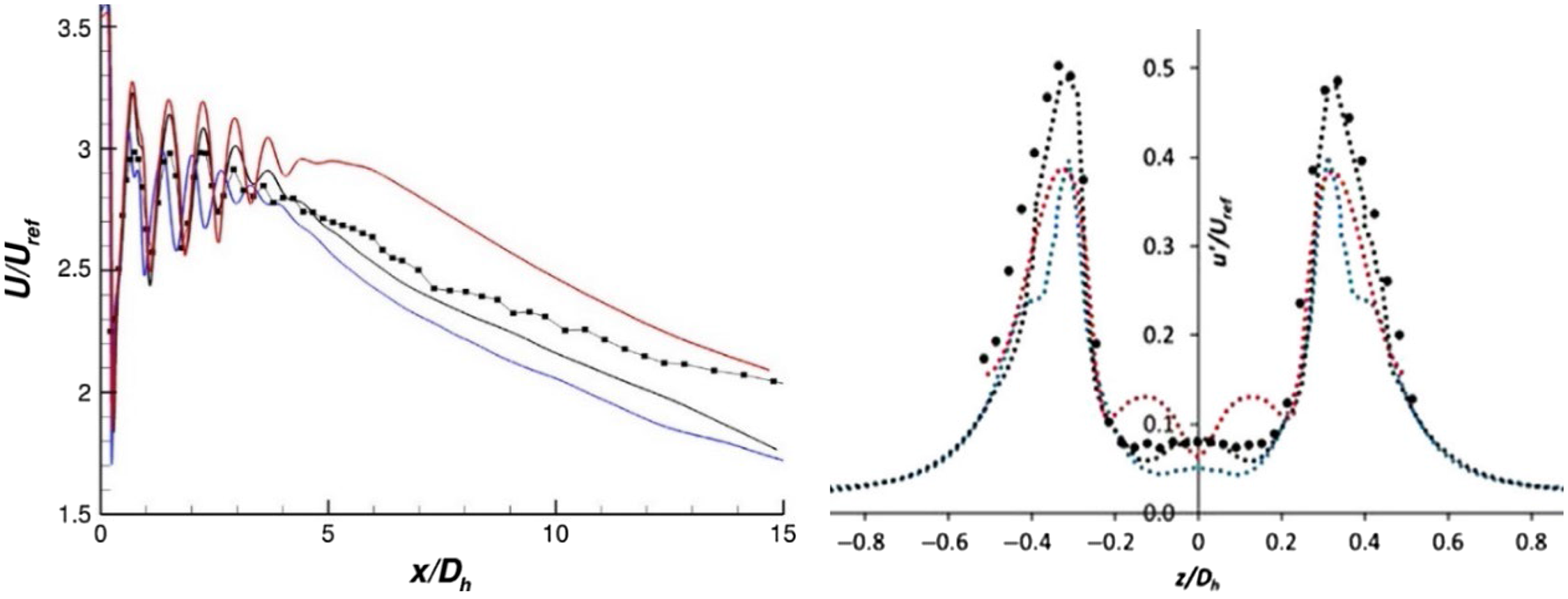
Figure 48. LES (blue/black, two SGS models) and RANS (red) axial velocity mean/rms versus experiments, from Ref. Reference Wang and McGuirk76.
No acoustic analysis was carried out in Ref. Reference Wang and McGuirk76, but the LES/measurement study of Chakrabarti et al. (Reference Chakrabarti, Unnikrishnan, Gaitonde, Stack, Baier, Karnam and Gutmark77) for an AR = 2 rectangular nozzle at overexpanded NPR = 3 and a hot jet NTR = 3.0 did include acoustics in both the simulation (LES/FWH approach) and measurement programme. Finer meshes were used with up to 300 × 106 mesh points, with a digital filtering method applied to generate LES inlet conditions. Figure 49 (left) presents an instantaneous picture visualising jet eddy structures (coloured by Mach number). Much attention was paid to the shock structure within the potential core, particularly as the simple bi-conic internal geometry of this nozzle produced a complicated set of interacting shock trains, some originating at the nozzle throat due to abrupt turning as well as those resulting from imperfect expansion at the nozzle exit. The complex structure of shock–shock interactions predicted is shown in Fig. 49 (right), including the appearance of a separation region (dark-grey area) just aft of the throat (although this would almost certainly have been designed out in practice). Agreement with the measured potential core length and initial velocity decay was good (Fig. 50, left), although the shock cell amplitude is underpredicted. This is surprising given the mesh density; this may be caused by inaccuracies associated with separation-induced nozzle total pressure loss, which was not confirmed by the external-only measurements. The predicted far-field OASPL levels were in very good agreement with measurements (Fig. 50, right), including the fact that the acoustic signature was effectively axisymmetric, due to the low AR of the test nozzle.

Figure 49. LES-predicted instantaneous eddy structure and shock cells from Ref. Reference Chakrabarti, Unnikrishnan, Gaitonde, Stack, Baier, Karnam and Gutmark77.
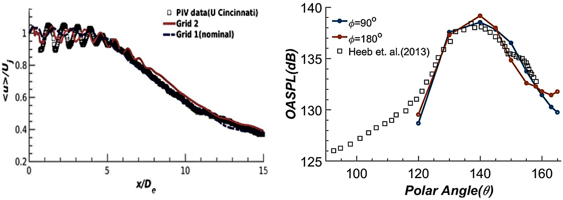
Figure 50. LES mean centreline velocity and far-field OASPL versus experiments from Ref. Reference Chakrabarti, Unnikrishnan, Gaitonde, Stack, Baier, Karnam and Gutmark77.
4.2 Installation effects (aft-deck, scarfing)
Close integration of nozzle geometry for military aircraft may result in significant interaction between airframe surfaces and jet plume development. Examples of this are: (i) the nozzle is recessed within the aft-body, and initial jet development takes place above a solid surface (often termed an ‘aft-deck’) which limits entrainment from below, and (ii) the nozzle sidewalls or upper/lower surfaces are cut at an angle to match faceted surface angles on the airframe, often termed ‘scarfing’. Behrouzi and McGuirk (Reference Behrouzi and McGuirk79,Reference Behrouzi, McGuirk and Avenell80) reported experimental studies illustrating the aerodynamic consequences of both of these options.
Aft-deck effects were studied in Ref. Reference Behrouzi and McGuirk79 using the rectangular high-AR (7.35) convergent-only nozzle (4/1 contraction) shown in Fig. 51 (top) in both ‘clean’ and with aft-deck geometry. The nozzle exit had a hydraulic diameter of D h = 22.46mm (used as a reference length for non-dimensionalisation), with a datum aft-deck length of 2.37D h (with 40% shorter and longer also being examined); several values of NPR were studied initially from choked (1.9) to moderately strong under-expansion (4.0), all at NTR = 1.0. The impact of the aft-deck was assessed first using colour Schlieren visualisation; two images for NPR = 3.0 and 4.0 are shown in Fig. 51. The appearance of shock cells is clearly seen; these grow in both length and amplitude as NPR increases. At NPR = 4, boundary-layer separation occurs before the aft-deck end is reached; the wall boundary layer is unable to sustain forward flow against the adverse pressure gradient caused by an oblique shock compression. Note also that the spatially varying pressure created by the shock cells on the aft-deck (in contrast to the constant ambient pressure on the jet upper surface) causes a net vertical force on the plume, which is deflected down when it leaves the aft-deck (but upwards at lower NPR).
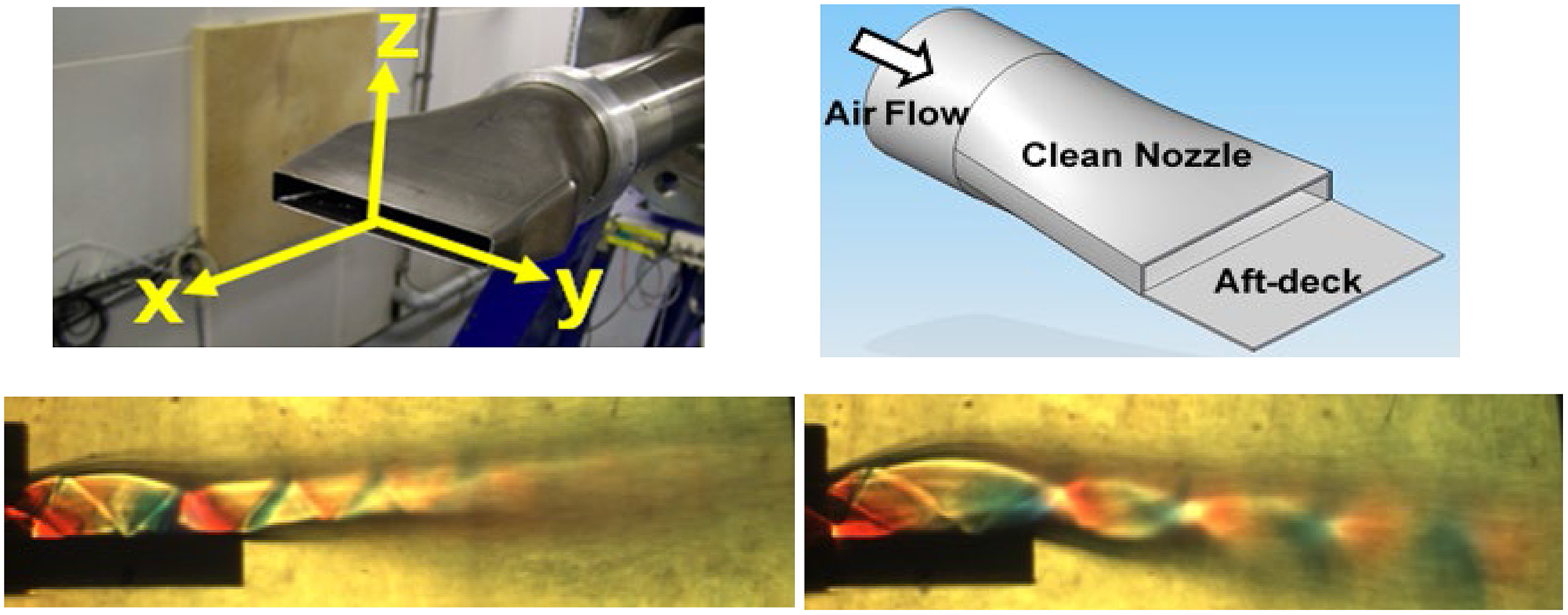
Figure 51. Clean and with aft-deck nozzle geometries and flow visualisation with NPR = 3 and 4 from Ref. Reference Behrouzi and McGuirk79.
Static pressure measurements on the aft-deck surface (Fig. 52, top) reveal the cause of separation and deflection events. The location of the strong adverse pressure gradient moves aft and strengthens for NPR > 2.5; for NPR > 4.5, a static pressure plateau appears, identifying the separation zone. LDA measurements made in Ref. Reference Behrouzi, McGuirk and Avenell80 are also shown in Fig. 52 (bottom) for NPR = 2.45, comparing the non-dimensional axial velocity on the nozzle minor axis plane. Reduced entrainment caused by the aft-deck is accompanied by increased axial penetration of the high jet velocity region, reduced lateral spreading, and asymmetric jet development, leading to the peak velocity moving upwards slightly from its original location on the nozzle geometric axis. These data represent a good test case for installation aerodynamic effects and were adopted as part of the AIAA 4th Propulsion Aerodynamic Workshop (Reference Crowe, Thornock and Brown81); Eight different CFD solutions were assessed, although only one adopted LES. The principal conclusion was that none of the results presented were able to capture the separating case quantitatively accurately, although the single LES result was the most promising. Shock wave–boundary layer separation modelling remains a challenging problem.
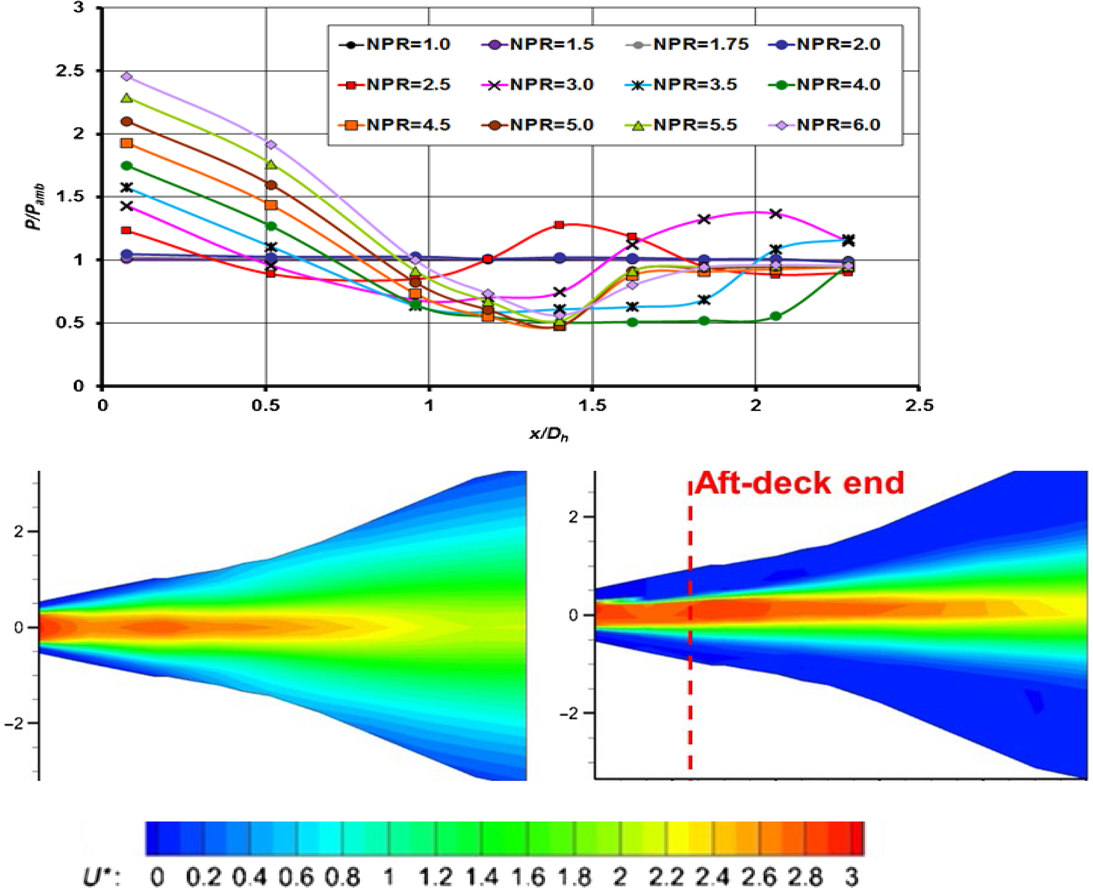
Figure 52. Aft-deck static pressure profiles, clean and with aft-deck axial velocity from Ref. Reference Behrouzi and McGuirk79.
To study the effect of scarfing (a nozzle exit plane non-orthogonal to the nozzle axis) on jet plume development (Reference Behrouzi, McGuirk and Avenell80) measurements were conducted on the geometry shown in Fig. 53 (top, where the red rectangle indicates that measurements were undertaken with the co-ordinate origin located at the throat plane). For comparison purposes, the datum un-scarfed geometry was the con-di rectangular nozzle used in Ref. Reference Behrouzi and McGuirk79 (Fig. 47, top left). A non-orthogonal exit plane was created by simply cutting back using a scarfing plane angled at 35° to the datum exit plane. The divergence length was increased slightly to ensure the nozzle exit area projected in the axial direction was equal to the clean nozzle exit area. No internal modifications were introduced to compensate for laterally varying expansion lengths in the diverging section of the nozzle as might be undertaken in practice. The nozzle design operating point was identified by Schlieren visualisation as the NPR providing the closest to a shock-free jet. For the clean nozzle, this NPR was 3.5; this reduced to 3.15 for the scarfed nozzle due to different losses/expansion conditions. Schlieren imaging at different NPRs is provided in Fig. 53. At NPR = 2.5, the clean nozzle displays an over-expanded pattern (first wave colour is green, with the terminating normal shock at the divergent duct exit being just visible, bending out into the plume), whereas at NPR = 4.0 the nozzle exit first shows under-expanded oblique shock waves (first wave colour red). With scarfing, the laterally variable expansion inside the nozzle creates more diffuse Schlieren images due to line-of-sight averaging of 3D wave structures, particularly near the nozzle; some evidence of internal expansion waves can also be seen.
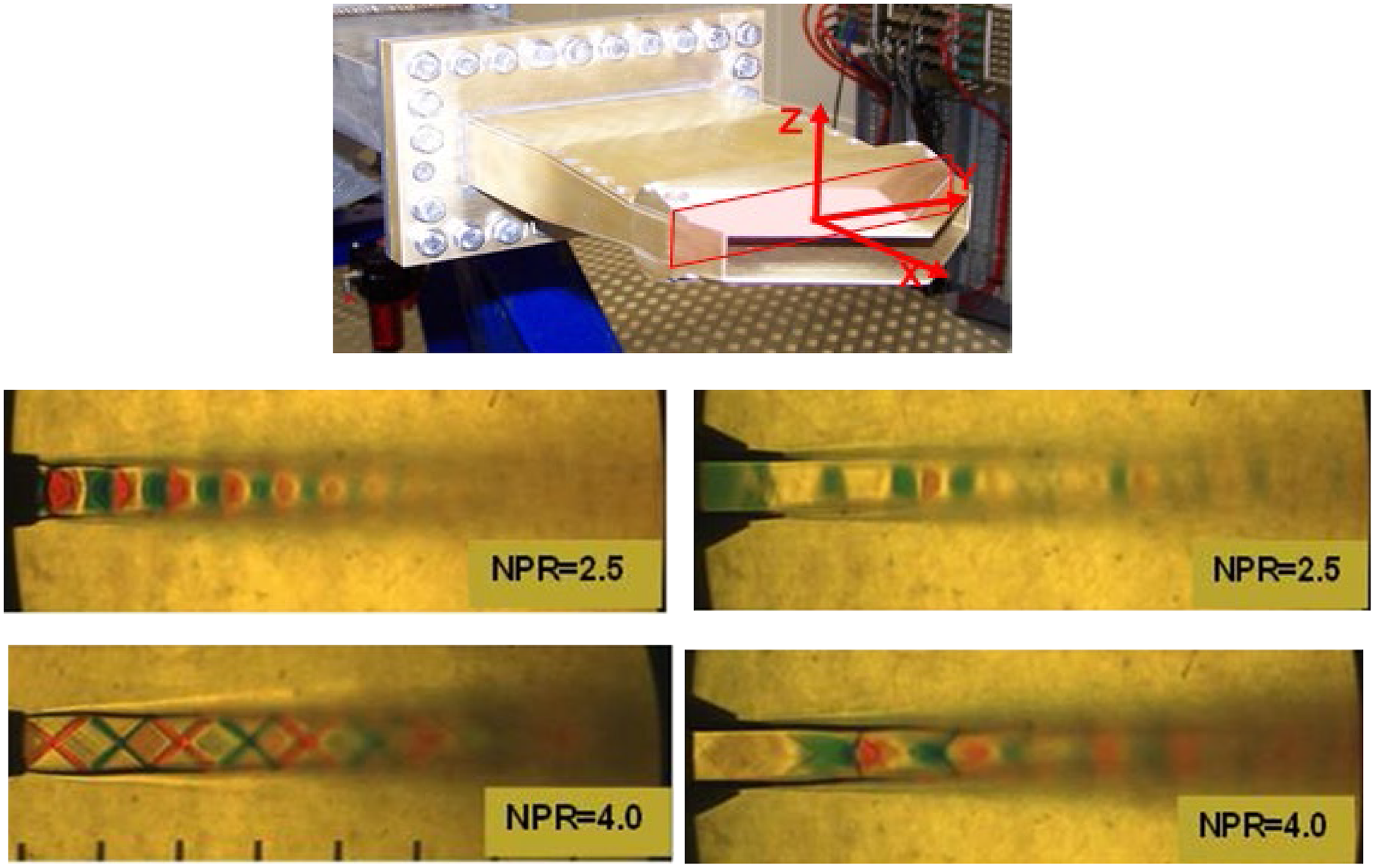
Figure 53. Scarfed nozzle geometry, flow visualisation of clean/scarfed nozzles from Ref. Reference Behrouzi, McGuirk and Avenell80.
LDA measurements and RANS (k–ɛ) predictions were also carried out in Ref. Reference Behrouzi, McGuirk and Avenell80 for both clean and scarfed nozzles. The scarfed nozzle results are shown in Fig. 54 for two off-design NPR values of 2.5 (left) and 4.0 (right). In the measurements, distinctive features caused by scarfing appear, which are not seen in the clean nozzle flow. These are a consequence of y–z plane secondary flows, which cause contour distortions near the symmetry plane (for both NPRs) and at the plume corners (for NPR = 4.0). The jet boundary shape is now influenced by these streamwise vorticity effects as well as turbulent diffusion. For NPR = 2.5, these processes combine to cause radically different spreading rates in the two cross-stream directions. At x/D h = 12.0, the jet cross-section aspect ratio has changed from 2:1 (half-section) to approximately 1:1, although it is still not axisymmetric. A small central high-velocity core is surrounded by lobes with larger penetration along major and minor axes. The plume edge has spread only marginally in the major axis direction from its location at nozzle exit, whereas it has moved substantially in the minor axis direction. For NPR = 4.0, the interplay between turbulent mixing and secondary velocity convection produces a quite different result: the plume retains its rectangular shape for the entire downstream distance, plume growth occurs in both cross-stream directions at similar rates with diffusion leading to rounded corners and a bifurcation also appears with off-centreline velocity peaks at x/D h = 12.0.
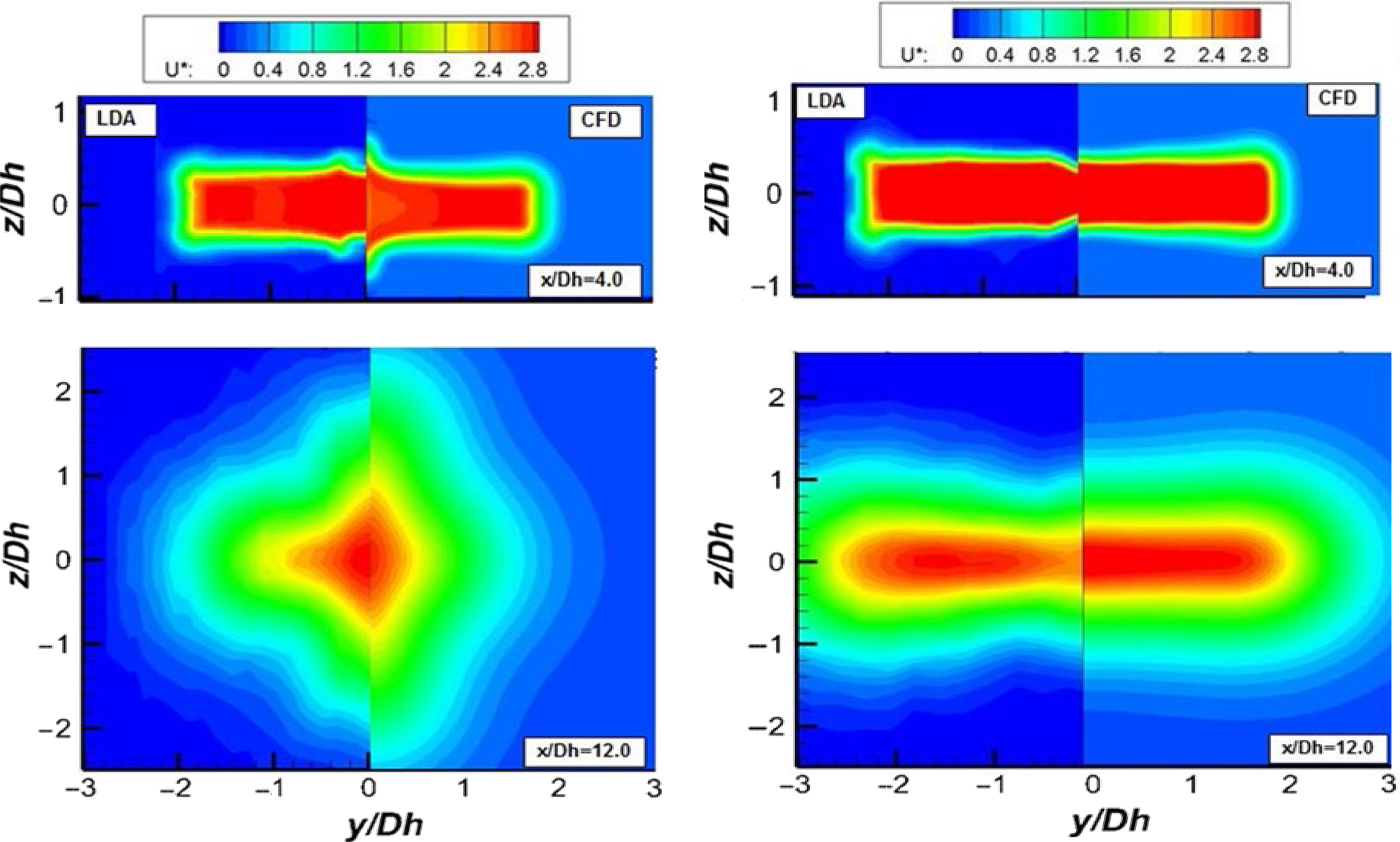
Figure 54. LDA and CFD data for scarfed nozzle with NPR = 2.5 (left) and 4.0 (right) from Ref. Reference Behrouzi, McGuirk and Avenell80.
Figure 54 shows that the measured trend is only qualitatively captured by RANS. A four-lobed shape is predicted to appear at over-expanded conditions, and a rectangular shape retained for under-expanded flow. The predicted secondary velocities which control the jet cross-section shape are shown in Fig. 55 as due to a clockwise vortex (looking upstream) near the y = 0 plane for over-expanded flow but an anti-clockwise vortex towards the nozzle upper corner for under-expanded conditions. Comparison of jet plume shapes indicates that the predicted secondary velocities are too strong at over-expanded conditions but under-predicted for NPR = 4.0. RANS correctly predicts a four-lobed shape for NPR = 2.5, but an overshoot compared with measurements is seen at x/D h =12.0 with the predicted z-direction extent of the plume exceeding the y-direction extent. The under-expanded case is also not correctly reproduced since no evidence of bifurcation is shown in the predicted velocity, unlike in the measured data; the depression seen in the measurements close to the y = 0 plane is also not visible in the CFD. Clearly, RANS cannot capture the details of scarfing observed in this experiment. It would be of interest to explore the capability of LES and to consider alternative scarfed geometries, which should include re-shaping of the internal nozzle geometry to offset the effects of different lateral expansion lengths.
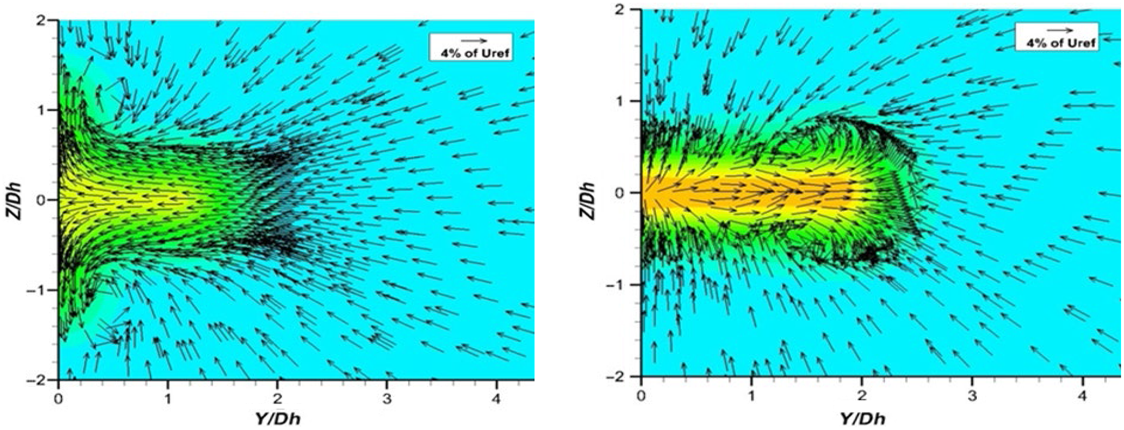
Figure 55. RANS secondary flow with scarfed nozzle, x/Dh = 7 and NPR = 2.5 (left) and 4.0 (right) from Ref. Reference Behrouzi, McGuirk and Avenell80.
4.3 Aeroacoustics – screech
The acoustic phenomenon referred to as screech in imperfectly expanded high-speed jets was first noted in the 1950s by Powell (Reference Powell82) and has been reviewed extensively by Edgington-Mitchell (Reference Edgington-Mitchell83). It involves a self-sustained feedback loop where an aeroacoustic resonance is sustained by disturbances (instability waves or turbulent eddies) in the jet shear layer, which convect downstream and interact with the shock cells, generating sound. This propagates upstream in the ambient (stagnant) medium, subsequently interacting with the shear layer at nozzle exit, producing a new downstream-travelling disturbance to continue the cycle. One of the original photographs of this phenomenon is shown in Fig. 56 (top left) for a rectangular jet at NPR = 3.5 with the acoustic wave origin located around the third or fourth shock cell. This image is taken from Alkislar et al. (Reference Alkislar, Krothapalli and Lourenco84), who used an AR = 4 con-di rectangular nozzle with design M
j
= 1.44 but operated at an over-expanded condition (M
j
= 1.69). The near-field acoustic spectrum obtained with a microphone is given in Fig. 56 (top right), showing the sound level in decibels versus the Strouhal number (based on the nozzle height h) for both the on-design and over-expanded conditions. The screech tone fundamental frequency and its harmonics are identified by the distinct peaks, standing some 20dB above the broadband noise; the absence of screech tones in the shock-free design condition is also evident. Alkislar et al. (Reference Alkislar, Krothapalli and Lourenco84) noted that the screech frequency reduced monotonically with U
j
but with a slightly different relationship for under- and over-expanded conditions, although the instability mode (flapping in minor axis direction) remained the same throughout. Similarly, the screech amplitude varied considerably, peaking at M
j
= 1.3 and 1.69 for under- and over-expanded flow. SPIV velocity measurements were made, showing that the jet plume exhibited strong axis-switching behaviour (Fig. 56, bottom right), the long dimension of the nozzle changing from vertical to horizontal in just 25h distance, noting also that this did not occur at the on-design NPR. The impact of the screech oscillation is also evident in fluctuating velocity measurements. Since a strong periodic component is present, fluctuations from the long time-mean velocity include contributions from the periodic motion as well as a turbulent contribution. Figure 56 (bottom right) presents the transverse (y-direction) mean normal Reynolds stress evaluated using different fluctuating components, where circles represent the periodic contribution, triangles the turbulence component and black squares the sum of both. It is clear that, up to the end of the potential core (
 $\sim$
x/h = 20), the dominant contribution measured by the SPIV system is from the periodic flapping motion (note that such peaks are not seen in the axial component).
$\sim$
x/h = 20), the dominant contribution measured by the SPIV system is from the periodic flapping motion (note that such peaks are not seen in the axial component).

Figure 56. Screech, appearance, frequency, velocity contours and turbulence from Ref. Reference Alkislar, Krothapalli and Lourenco84.
Although the above data seem the ‘gold standard’ for CFD validation, they do not appear to have been exploited to this end to date. However, Wu et al. (Reference Wu, Lele and Jeun85) applied the high-speed LES/FWH method of Brès et al. (Reference Brés, Ham, Nichols and Lele75) described in Subsection 4.1 to analyse the 4:1 rectangular nozzle studied experimentally by Valentich et al. (Reference Valentich, Upadhayay and Kumar86) and designed for a perfectly expanded M j = 1.44 (NPR = 3.37). Very similar flow and screech behaviour was observed as in Ref. Reference Alkislar, Krothapalli and Lourenco84, with axis switching, high-amplitude tonal noise and flapping oscillations evident in unsteady statistics. Three over-expanded cases were simulated with M j = 1.56, 1.69 and 1.78, using coarse, medium and fine meshes with 50, 140 and 280 × 106 cells. Results with the two finer meshes were in agreement, and the 140 × 106 mesh was run for longer to increase accuracy for low frequencies. The nozzle geometry is presented in Fig. 57 (top left), and the excellent comparison between LES and SPIV measurements (for the M j = 1.69 case that produced the highest screech amplitudes) is demonstrated in Fig. 57 (top right) via time-mean axial velocity contours in both minor and major axis planes.
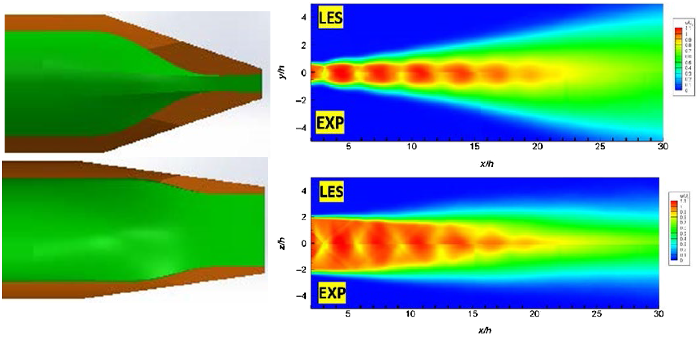
Figure 57. Nozzle geometry and LES/PIV comparison for mean axial velocity from Ref. Reference Wu, Lele and Jeun85.
Similar good agreement was obtained for turbulent statistics. Two examples are provided here to demonstrate this. In Fig. 58 (left), the top graph shows the transverse rms fluctuation (minor axis direction) whereas the bottom picture is for axial rms. As noted above, the screech flapping motion contributes significantly to the transverse fluctuation but only appears to influence the axial fluctuation weakly. The simulation results are in very good quantitative agreement with the measured data for both components. Finally, a noise spectrum on the minor axis plane at 90° to the centreline and 25h from nozzle exit is given in Fig. 58 (right) The shape, broadband and tonal characteristics seen in the measurements are reproduced well in the simulation up to St = 1. LES captures the first two harmonics of the screech tone, although at a slightly higher frequency and lower amplitude. Poor agreement for higher frequencies is typical of current LES/FWH capabilities, even with the very fine mesh densities used in this example. The quality of the screech prediction in high-speed jets in these results is similar to that achieved by the subsonic noise predictions presented in the previous section.
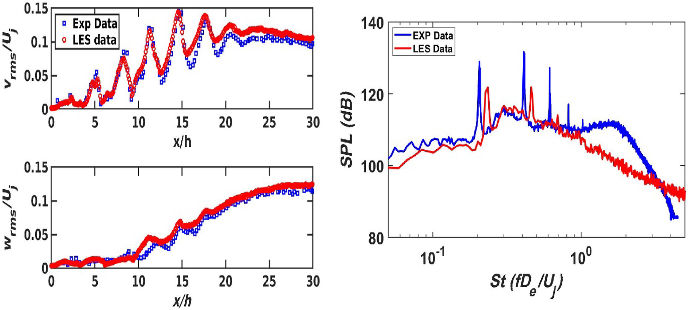
Figure 58. Fluctuating rms and noise PSD compared with measured data in screeching jet from Ref. Reference Wu, Lele and Jeun85.
4.4 Design for noise reduction
The noise from high-speed jets in operational scenarios involving launch/landing of carrier-based aircraft is clearly a major concern and has driven design efforts to mitigate high acoustic levels. Several technology concepts have been explored, for example the use of bevelled nozzles (Reference Viswanath and Czech87,Reference Viswanath, Spalart, Czech, Garbaruk and Shur88) and tabbed nozzles (Reference Tam and Zaman89). More favoured recently, principally due to their ability to be switched off to avoid performance losses during flight, are variations of the active control application of ‘fluid tabs’ (Reference Behrouzi, Feng and McGuirk90), successfully applied to supersonic jets by Prasad and Morris (Reference Prasad and Morris91,Reference Prasad and Morris92). Multiple injectors using air bled off the by-pass stream are located in the divergent section of the nozzle. The placement/pressure ratio of the injectors can be adjusted to weaken the shock structures that contribute to broadband shock noise but also introduce streamwise vorticity to enhance jet mixing and bring about changes to the large-scale turbulent structures that are dominant jet broadband noise sources. An LES study with a mesh of 18 × 106 cells (considered accurate up to St = 1.8) has been used to assess the introduction of this technology into a sub-scale model of the GE F404 engine nozzle shown in Fig. 59 for which far-field acoustic data are available. The baseline nozzle geometry consists of 12 interleaved facetted surfaces, with a throat-to-exit area ratio fixed for the LES study at a design M j =1.65 but operated at NPR = 3.0 (M j = 1.36, a simulated take-off condition) and with a hot jet at NTR = 3.0. Two rows of three injectors spaced azimuthally uniformly were placed at particular injection angles and distances from the throat in the configuration shown in Fig. 59 that was found to be most effective in terms of peak noise reduction.
Figure 59. Scale model of F404 nozzle with fluid injector inserts from Refs Reference Prasad and Morris91, Reference Prasad and Morris92.
Figure 60 illustrates LES-predicted instantaneous density gradient and pressure wave contours for both clean (left) and with injector (right) simulations. The injector flows disrupt the coherence of the oblique shock waves and enhance mixing within the shear layer. The predicted acoustic PSD at two polar angles is given in Fig. 60 (bottom left). Good agreement is observed up to St
 $\sim$
1, as was observed in subsonic LES. A comparison of the simulations and measurements for the OASP directivity curve is given in Fig. 60 (bottom right), which also shows the sensitivity to mesh density; a coarse mesh of 3 × 10⁶ cells shows significant departure from measured data, but the medium (13 × 106) and fine (18 × 106) meshes produce similar, good performance. An estimate of thrust losses was also undertaken in Ref. Reference Prasad and Morris91, indicating that the noise reduction offered by the fluid injection technology was less than 1.5%, described as ‘very promising’. These results indicate that LES/FWH holds much promise for contributing to further development of this technology.
$\sim$
1, as was observed in subsonic LES. A comparison of the simulations and measurements for the OASP directivity curve is given in Fig. 60 (bottom right), which also shows the sensitivity to mesh density; a coarse mesh of 3 × 10⁶ cells shows significant departure from measured data, but the medium (13 × 106) and fine (18 × 106) meshes produce similar, good performance. An estimate of thrust losses was also undertaken in Ref. Reference Prasad and Morris91, indicating that the noise reduction offered by the fluid injection technology was less than 1.5%, described as ‘very promising’. These results indicate that LES/FWH holds much promise for contributing to further development of this technology.
Figure 60. Predicted versus measured PSD and OASPL curves from Refs Reference Prasad and Morris91, Reference Prasad and Morris92.
4.5 Powered lift jet aerodynamics
Powered lift aircraft such as the British Aerospace Sea Harrier FRS1 and the Lockheed Martin F-35 Lightning II place special demands on the propulsion system. Manoeuvres such as hovering out of ground effect and the transition between wing-borne and jet-borne flight, and the associated jet-in-crossflow related aerodynamic interference for STOVL aircraft, have been described and reviewed extensively by Saddington and Knowles (Reference Saddington and Knowles93) and Kuhn et al. (Reference Kuhn, Margason, Curtis and Lu94) Even more complex fluid mechanics governs the in-ground-effect phase of flight when the propulsive jet interacts with both the airframe and ground plane. Full understanding of this is essential to achieve acceptable vertical landing capability. Three important in-ground-effect aerodynamic problems are: (i) the fountain effect, (ii) the ground vortex and (iii) hot gas re-ingestion (HGI). Figure 10 (right) illustrates the essential characteristics of near-ground aerodynamics. The ground vortex occurs when the onset flow, created by headwinds or forward aircraft motion, interacts with the forward-flowing wall sheet created after impingement of jet exhaust plumes on the ground plane. The location of the top edge of this vortex relative to the engine intake controls the occurrence and strength of HGI, which can cause thrust loss, compressor stall and engine surge. A fountain flow is created by multiple lift jets impinging on the ground plane, forming initially separate 3D wall jets that subsequently collide to produce an upward flow (fountain upwash). Impingement on the underside of the aircraft creates a force that influences aircraft pitching moment and hence stability and control; also, if this flow is partially directed forwards towards the intake, it may contribute to HGI. Sometimes, special devices (‘strakes’ and ‘dams’) are included on the aircraft to capture/deflect this flow. Design was originally dominated by information gained from model-scale rig testing; later, RANS was helpful in providing data on the ground vortex and turbulent mean flow but was unable to provide insight into important phenomena associated with the highly unsteady fountain flow, HGI and associated unsteady flow distortion and swirl in the engine intake. Interest has therefore grown in the ability of LES to produce more accurate prediction of ground-effect aerodynamics.
Behrouzi and McGuirk (Reference Behrouzi and McGuirk95) investigated the intake ingestion problem using LDA and a water-tunnel experiment to facilitate Laser-Induced Fluorescence (LIF) flow visualisation of unsteady motion and provide CFD validation data. The near-ground phenomena described are unlikely to contain high-Mach-number compressibility effects, so the use of a water flow facility should be acceptable if non-dimensional parameters such as the ratio of impinging jet velocity to onset flow velocity (R = V j /U on) are maintained. This was confirmed in Ref. Reference Behrouzi and McGuirk95 by comparing the measured variation of the ground vortex forward penetration with R in water flow with published airflow experiments. Very good agreement was obtained for R varying between 15 and 35, covering the relevant range for STOVL aircraft. The experimental configuration is presented in Fig. 61 (top left). Two vertical jets with a spacing of 6d j were arranged above the horizontal floor of a water tunnel at an impingement height of 7d j ; a circular intake with diameter of 3d j was located between the jets, with the intake diameter and their vertical and horizontal spacing relative to the jet nozzle exits chosen to be non-dimensionally similar to a Harrier aircraft. The return pipe of the intake was connected to the pump supplying the jet nozzles to maintain equal and steady-state mass flow conditions.
Figure 61. LDA water flow study of intake ingestion from Ref. Reference Behrouzi and McGuirk95.
A velocity ratio of R = 24 was selected for detailed study of both mean and turbulence statistics, but only the profile in Fig. 61 (top right) is included here to illustrate the jet and fountain mean vertical velocity fields. A lateral profile is measured along the line y/d j = 2.0 from the central symmetry plane (z/d j = 0.0) to just outboard of an impinging jet (note that positive velocity here indicates downward motion). This line was chosen as it contains both the maximum upwash and peak jet velocity just before the start of impingement deceleration begins; capturing both of these was considered to be an important validation test. An impression of the highly unsteady ingestion process is provided in Fig. 61 (bottom); three images are shown from a video of light emission when a fluorescing dye was included in the impinging jet water flow and illuminated with a laser light sheet. Large-scale fluctuating structures are visible, with the top edge of the mixed fluid varying from below the intake to well above it.
The LES study of this data is reported in Ref. 96 (Fig. 62). The instantaneous snapshots show the complex unsteady ground vortex and impingement flows with transient large-scale structures similar to those seen in Fig. 61. Evidence of lateral fountain motion is suggested in the upwash fountain and confirmed by the PSD of predicted lateral fluctuations for a point on the symmetry plane at the bottom of the fountain in Fig. 62 (left, bottom), indicating a strong flapping motion at a frequency of 1,650Hz. Examples of comparison of mean velocity profiles between the simulation and the LDA measurements of Ref. Reference Li, Page and McGuirk96 are given in Fig. 62 (right). LES is shown to provide better accuracy than RANS for the lateral profile of vertical velocity (top), and the peak upwash velocity and its decay (bottom).
Figure 62. Simulation of intake ingestion: instantaneous contours, comparison with data from Ref. Reference Li, Page and McGuirk96.
Encouraged by these intake ingestion results, simulation of a full aircraft geometry (at operating conditions representative of a wheels-on-ground condition) was carried out and is described by Page and McGuirk (Reference Page and McGuirk97). The geometry of a 1:5 scale model of an AV-8B/GR-7 Harrier located in a test cell at Rolls-Royce (Bristol) was made available. Airflow to the four nozzles and extraction of air from the intake required extra tubes installed above the model, and these were included in the simulation, as shown in Fig. 63. Operating conditions for the rear jets comprised an NPR of 2.0 and temperature of 700K; for the forward jets, NPR = 2.5 and 350K were specified. The ambient onset velocity was 6m/s at ambient temperature, and the intake static pressure was set at 3kPa below ambient. The LES mesh included
 $\sim$
17.5 × 10⁶ nodes; this simulation is now more than 10 years old, so a finer mesh could certainly be afforded now.
$\sim$
17.5 × 10⁶ nodes; this simulation is now more than 10 years old, so a finer mesh could certainly be afforded now.
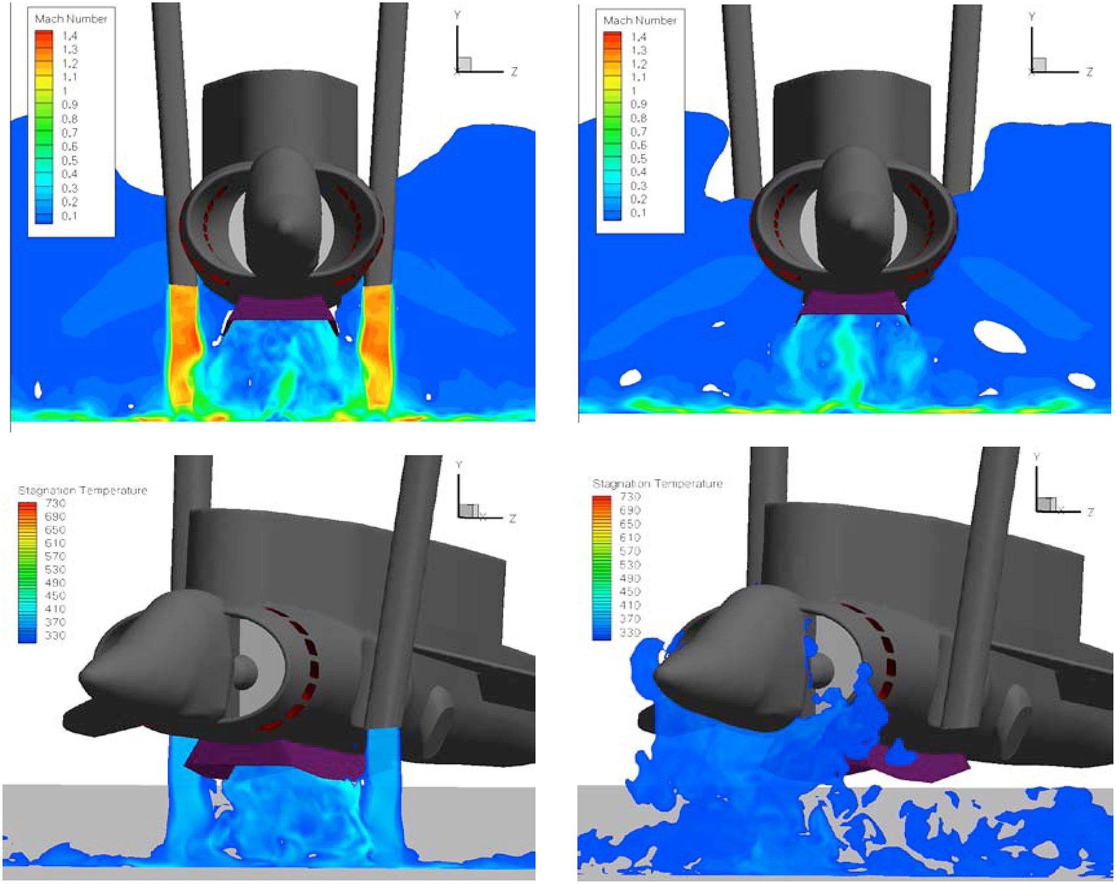
Figure 63. Instantaneous LES snapshots of velocity (top) and temperature (bottom) fields from Ref. Reference Page and McGuirk97.
Figure 63 provides some instantaneous snapshots from a video of the simulation. The top shows two images of the velocity field selected to display the fountain flow behaviour. Lateral fountain flapping was again observed in this full-geometry simulation; the top left image is for a plane through the front jets and shows the fountain in its furthest deflection to the right; in other images, a similar leftward deflection was seen. The top right image is for a plane just in front of the dam device and shows the strakes/dam capturing and channelling backwards the fountain flow. Note also the relatively thin ground wall sheet. The instantaneous contours for total temperature (bottom) visualise the hot gas ingestion process. At the front jet plane, the fountain flow is still at
 $\sim$
400K and the capturing/shielding effect of the underside devices is active; at the intake plane, the large turbulent eddy structures at the top of the ground vortex have brought the hot gas right up in front of the whole intake area, and ingestion is taking place. Quantitative validation of the results of this simulation were not provided, but the realism of the results is very encouraging. In reality, the aircraft is also in motion towards the ground plane in a landing manoeuvre, and this has been reproduced in RANS CFD by Richardson et al. (Reference Richardson, Dawes and Savill98). It would be interesting to investigate this transient effect in LES.
$\sim$
400K and the capturing/shielding effect of the underside devices is active; at the intake plane, the large turbulent eddy structures at the top of the ground vortex have brought the hot gas right up in front of the whole intake area, and ingestion is taking place. Quantitative validation of the results of this simulation were not provided, but the realism of the results is very encouraging. In reality, the aircraft is also in motion towards the ground plane in a landing manoeuvre, and this has been reproduced in RANS CFD by Richardson et al. (Reference Richardson, Dawes and Savill98). It would be interesting to investigate this transient effect in LES.
5.0 Summary and conclusions
The combination of increasingly strict civil aerospace noise regulations and the high-order turbulence statistics that are key to jet noise generation has encouraged the search for alternatives to two-equation RANS statistical turbulence models, which have been the industry standard for more than 30 years. Growth in by-pass ratio (nacelle diameter) also increases interference between jet plume and wing/deployed flap surfaces, with aerodynamic and aeroacoustic consequences that must be addressed. For military aircraft, the design demands are different but point in the same direction: a need for better turbulence modelling and improved aeroacoustic analysis methods. In this application, it is accurate prediction of the supersonic jet potential core length for different nozzle exit geometries (for reduced IR signature) and avoidance of high screech acoustic levels that are the principal design drivers. Both of these design problems involve the jet plume near field; this further increases the predictive challenge because standard RANS turbulence models have been calibrated more for self-similar flows. In addition, specific nozzle exit conditions, rarely known in practice and until recently typically not measured in laboratory-based experiments, increase in importance. Given the importance of this challenge, the survey provided here is intended to review work on the development/validation of predictive techniques for propulsive jet aerodynamics and aeroacoustics, summarise progress and suggest areas where further work is required.
Consideration of fluid mechanical and aeroacoustic aspects of propulsive jets revealed several important phenomena for modelling to address. For aerodynamics these include the velocity ratio, Mach-number-dependent compressibility and density ratio (hot jet) effects on shear-layer spreading rates; nozzle-related effects that determine important jet flow initial conditions (Reynolds number and acceleration-induced relaminarisation) and supersonic flow with possible embedded expansion/compression waves. For aeroacoustics, the principal sources of difficulty are the need to capture fourth-order space/time turbulence statistics and identify optimum numerical techniques for high spatial resolution to capture turbulent noise sources in the jet flow and subsequently propagate these accurately to the far field.
Results have been shown that indicate the superiority of the LES approach over the conventional RANS methodology. LES can demonstrate successful capture of all the effects that require special attention in RANS statistical turbulence models. Further, when LES is combined with a propagation technique (the most popular being the FWH approach), it can produce noise PSDs and OASPL directivity curves in a wide range of jet flows. Tremendous progress in predictive capability has been demonstrated across a range of test cases chosen from both civil and military aerospace via validation comparisons against specially conducted representative experiments with increasing realism. The most realistic and impressive example that (i) considered both by-pass and core nozzles, (ii) installed in an engine nacelle with pylon, (iii) attached to a lifting wing with deployed flaps and (iv) for the by-pass flow allowed consideration of upstream, internal engine turbomachinery and component hardware effects to establish nozzle exit conditions. Whilst these internal engine effects were not fully resolved but introduced via a body force model, this has certainly brought the LES/FWH approach to the level of a realistic design exercise.
However, further work is still required. It is important to note that much of the progress shown above has only been made possible because of the increase in size and improvement in access to high-performance, massively parallel compute clusters. Access to HPC facilities will grow but will still impede progress for some time. Turnaround time is still too long to allow LES methods to be routinely and regularly deployed in the design cycle. Areas for future development are therefore considered to be:
-
(i) The optimum industrial approach is inevitably to retain RANS for repetitive and fast turnaround design activities, restricting LES to selected final design stage investigations where high fidelity is essential. An important task therefore is to find ways of following the ‘LES-informed RANS’ route demonstrated in Refs Reference Karabasov, Afsar, Hynes, Dowling, McMullan, Pokora, Page and McGuirk46, Reference Depuru Mohan, Dowling, Karabasov, Xia, Graham, Hynes and Tucker67, whereby information from LES predictions is used to improve RANS capability. This was applied to aeroacoustics in Refs Reference Karabasov, Afsar, Hynes, Dowling, McMullan, Pokora, Page and McGuirk46, Reference Depuru Mohan, Dowling, Karabasov, Xia, Graham, Hynes and Tucker67, but similar improved accuracy for RANS turbulent mixing is needed. One important example in the current context is the interplay between compressibility and hot jet effects, which dominates near-field turbulent mixing. The impact of this on the potential core length was also underlined in the analysis presented in Ref. Reference McGuirk and Feng18. LES captures these effects correctly, but no RANS turbulence model has yet convincingly demonstrated this capability. The measurements of Ref. Reference McGuirk and Feng18 provide an obvious validation data set for this. Machine-learning/data-driven approaches (Reference Duraisamy, Iaccarino and Xiao99) should also be utilised in this task.
-
(ii) The high-frequency limitation of the LES/FWH approach has been obvious in many examples presented. This is not amenable to improvement by simple mesh refinement to increase accuracy for higher Strouhal numbers, introducing the risk of excessive computational cost that will lead to inadequate sampling time for low frequencies. This represents a core challenge for LES aeroacoustics, that is, simultaneously avoiding numerical dissipation of high-frequency noise while affording long-time-duration sampling for adequate statistical accuracy of low-frequency noise. Promising ideas are starting to appear, including spectral broadening (Reference Angelino, Xia and Page53), the APE approach (Reference Moratilla-Vega, Lackhove, Janicka, Xia and Page52) and numerical methods making use of GPUs (Reference Markesteijn and Karabasov58) to make long simulation times affordable. The propagation technique adopted in Refs Reference Karabasov, Afsar, Hynes, Dowling, McMullan, Pokora, Page and McGuirk46, Reference Depuru Mohan, Dowling, Karabasov, Xia, Graham, Hynes and Tucker67 also indicates better high-frequency performance. None of these have yet definitely demonstrated success, but efforts to explore and contrast these alternatives are a high priority, since improved high-frequency resolution is crucial.
-
(iii) The importance of nozzle exit conditions in both experimental and computational studies of high-Re propulsive jet near-field flows has been clearly shown. These influence the potential core length and turbulence development in the thin shear layer immediately downstream of the nozzle exit (hence this region’s contribution to high-frequency noise). Recommendations for laboratory-based experimental studies include the use of minimum nozzle exit Re j O(106) (to avoid laminar boundary layers) and the inclusion of engine-representative internal nozzle acceleration (to capture possible relaminarisation effects). The implication for LES is that starting at the nozzle inlet should become the norm, with the actual nozzle geometry included in the simulation, which will also demand careful design of the internal near-wall mesh and the adoption of wall-stress SGS models that are capable of capturing near-wall length scales and relaminarisation effects.
-
(iv) The advance made in Ref. Reference Tyacke, Mahak and Tucker71 to extend the CFD analysis inside the engine needs to be properly validated (see (v) below). If confidence in the viability of this approach is thereby provided, it should be extended to the core nozzle by applying it downstream of the LP turbine. This is the best route for engineering applications to meet the requirements of (iii) for an accurate specification of nozzle exit conditions/accurate high-frequency noise capture. ‘Forcing’ of LES solutions to achieve a desired mean flow field has already been successfully demonstrated by fixing the mean pressure gradient for fully developed channel flows, and the R2M approach of Ref. Reference Morris and Farassat43 to force specified mean velocity profiles in LES inlet condition generation. The option to extend the body force technique used within a RANS method in Ref. Reference Tyacke, Mahak and Tucker71 to the LES level to improve the fidelity of the turbulence field entering the nozzle should thus also be explored.
-
(v) The successful progress described in Sections 3 and 4 would not have been possible without high-quality experimental validation data. There is an ongoing requirement for well-chosen validation experiments, using increasingly realistic/representative geometries. For comprehensive validation of unsteady LES CFD, more extensive data on spectral as well as spatial and temporal turbulence correlations are needed.
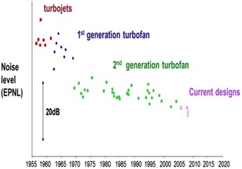
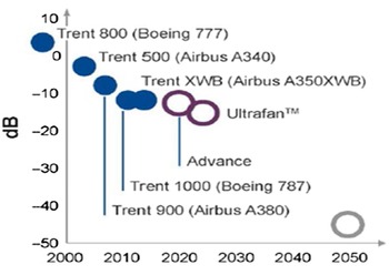


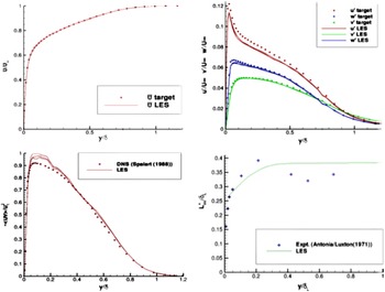
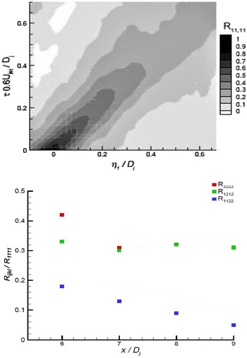


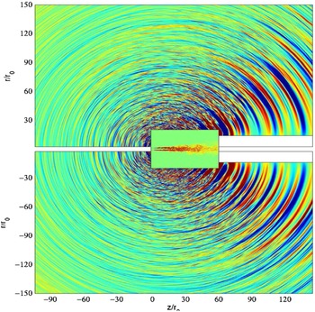

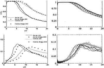


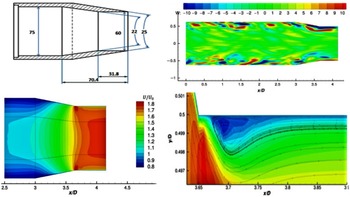


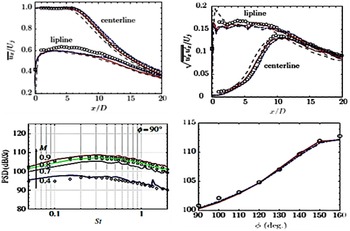


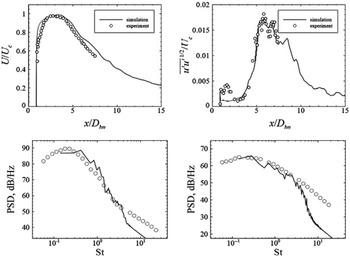

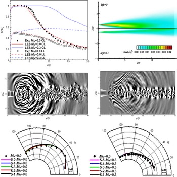


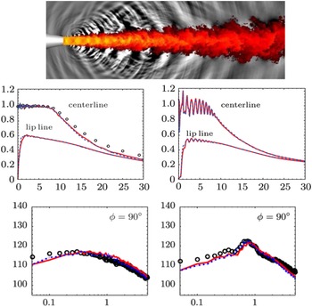


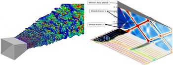


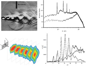

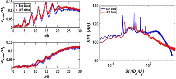


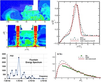


 Open access