


1 Introduction
Non-local integrable non-linear Schrödinger (NLS) equations are generated from matrix spectral problems under specific symmetric reductions on potentials [Reference Ablowitz and Musslimani3]. The corresponding inverse scattering transforms have been recently presented, under zero or non-zero boundary conditions, and there still exist N-soliton solutions in the non-local cases [Reference Ablowitz, Luo and Musslimani2, Reference Ablowitz and Musslimani4, Reference Gerdjikov and Saxena15]. Such soliton solutions can be constructed more generally from the Riemann–Hilbert problems with the identity jump matrix [Reference Yang51] and by the Hirota bilinear method [Reference Gürses and Pekcan16]. Some vector or matrix generalisations [Reference Ablowitz and Musslimani5, Reference Fokas10, Reference Ma32] and other interesting non-local integrable equations [Reference Ji and Zhu20, Reference Song, Xiao and Zhu44] were also presented. We would like to propose a class of general non-local reverse-space matrix NLS equations and analyse their inverse scattering transforms and soliton solutions through formulating and solving associated Riemann–Hilbert problems.
The Riemann–Hilbert approach is one of the most powerful approaches for investigating integrable equations and particularly constructing soliton solutions [Reference Novikov, Manakov, Pitaevskii and Zakharov42]. Many integrable equations, such as the multiple wave interaction equations [Reference Novikov, Manakov, Pitaevskii and Zakharov42], the general coupled non-linear Schrödinger equations [Reference Wang, Zhang and Yang46], the generalised Sasa–Satsuma equation [Reference Geng and Wu13], the Harry Dym equation [Reference Xiao and Fan47] and the AKNS soliton hierarchies [Reference Ma27], have been studied by formulating and analysing their Riemann–Hilbert problems associated with matrix spectral problems.
A general procedure for formulating Riemann–Hilbert problems can be described as follows. We start from a pair of matrix spectral problems, say,
 \begin{equation} -i \phi_x=U\phi,\ -i\phi_t=V\phi, \ U=A(\lambda)+ P(u,\lambda),\ V=B(\lambda) +Q(u,\lambda),\end{equation}
where i is the unit imaginary number,
 $\lambda $
is a spectral parameter, u is a potential and
$\lambda $
is a spectral parameter, u is a potential and
 $\phi$
is an
$\phi$
is an
 $m\times m$
matrix eigenfunction. The compatibility condition of the above two matrix spectral problems, that is, the zero curvature equation:
$m\times m$
matrix eigenfunction. The compatibility condition of the above two matrix spectral problems, that is, the zero curvature equation:
 \begin{equation}U_t-V_x+i[U,V]=0,\end{equation}
where
 $[\cdot,\cdot]$
is the matrix commutator, presents an integrable equation. To establish an associated Riemann–Hilbert problem for the above integrable equation, we adopt the following equivalent pair of matrix spectral problems:
$[\cdot,\cdot]$
is the matrix commutator, presents an integrable equation. To establish an associated Riemann–Hilbert problem for the above integrable equation, we adopt the following equivalent pair of matrix spectral problems:
 \begin{equation}\psi_x=i[A(\lambda) , \psi] +\check P(u,\lambda) \psi,\ \psi_t=i[B(\lambda),\psi ]+\check Q(u,\lambda)\psi,\ \check P=iP,\ \check Q=iQ,\end{equation}
where
 $\psi$
is also an
$\psi$
is also an
 $m\times m$
matrix eigenfunction. We often assume that A and B are constant commuting
$m\times m$
matrix eigenfunction. We often assume that A and B are constant commuting
 $m\times m$
matrices, and P and Q are trace-less
$m\times m$
matrices, and P and Q are trace-less
 $m\times m$
matrices. The equivalence between (1.1) and (1.3) follows from the commutativity of A and B. The properties
$m\times m$
matrices. The equivalence between (1.1) and (1.3) follows from the commutativity of A and B. The properties
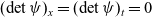 $(\det \psi )_x\,{=}\,(\det \psi )_t\,{=}\,0$
are two consequences of
$(\det \psi )_x\,{=}\,(\det \psi )_t\,{=}\,0$
are two consequences of
 $\textrm{tr}P=\textrm{tr}Q=0$
. There exists a direct connection between (1.1) and (1.3):
$\textrm{tr}P=\textrm{tr}Q=0$
. There exists a direct connection between (1.1) and (1.3):
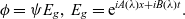 \begin{equation} \phi=\psi E_g,\ E_g= \textrm{e}^{iA(\lambda)x+iB(\lambda)t}.\end{equation}
It is important to note that for the pair of matrix spectral problems in (1.3), we can impose the asymptotic conditions:
 \begin{equation}\psi^{\pm}\to I_m,\ \textrm{when}\ x \ \textrm{or}\ t \to \pm \infty,\end{equation}
where
 $I_m$
stands for the identity matrix of size m. From these two matrix eigenfunctions
$I_m$
stands for the identity matrix of size m. From these two matrix eigenfunctions
 $\psi^\pm$
, we need to pick the entries and build two generalised matrix Jost solutions
$\psi^\pm$
, we need to pick the entries and build two generalised matrix Jost solutions
 $T^\pm(x,t,\lambda)$
, which are analytic in the upper and lower half-planes
$T^\pm(x,t,\lambda)$
, which are analytic in the upper and lower half-planes
 $\mathbb{C}^+$
and
$\mathbb{C}^+$
and
 $\mathbb{C}^-$
and continuous in the closed upper and lower half-planes
$\mathbb{C}^-$
and continuous in the closed upper and lower half-planes
 $\mathbb{\bar C}^+ $
and
$\mathbb{\bar C}^+ $
and
 $\mathbb{\bar C}^-$
, respectively, to formulate a Riemann–Hilbert problem on the real line:
$\mathbb{\bar C}^-$
, respectively, to formulate a Riemann–Hilbert problem on the real line:
 \begin{equation}G^+(x,t,\lambda)=G^-(x,t,\lambda) G_0(x,t,\lambda),\ \lambda \in \mathbb{R},\end{equation}
where two unimodular generalised matrix Jost solutions
 $G^+$
and
$G^+$
and
 $G^-$
and the jump matrix
$G^-$
and the jump matrix
 $G_0$
are generated from
$G_0$
are generated from
 $T^+$
and
$T^+$
and
 $T^-$
. The jump matrix
$T^-$
. The jump matrix
 $G_0$
carries all basic scattering data from the scattering matrix
$G_0$
carries all basic scattering data from the scattering matrix
 $S_g(\lambda )$
of the matrix spectral problems, defined through
$S_g(\lambda )$
of the matrix spectral problems, defined through
 \begin{equation} \psi^-E_g=\psi ^+E_gS_g(\lambda ) .\end{equation}
Solutions to the associated Riemann–Hilbert problems (1.6) provide the required generalised matrix Jost solutions in recovering the potential of the matrix spectral problems, which solves the corresponding integrable equation. Such solutions
 $G^+$
and
$G^+$
and
 $G^-$
can be presented by applying the Sokhotski–Plemelj formula to the difference of
$G^-$
can be presented by applying the Sokhotski–Plemelj formula to the difference of
 $G^+$
and
$G^+$
and
 $G^-$
. A recovery of the potential comes from observing asymptotic behaviours of the generalised matrix Jost solutions
$G^-$
. A recovery of the potential comes from observing asymptotic behaviours of the generalised matrix Jost solutions
 $G^\pm$
at infinity of
$G^\pm$
at infinity of
 $\lambda $
. This then completes the corresponding inverse scattering transforms. Soliton solutions can be worked out from the reflectionless transforms, which correspond to the Riemann–Hilbert problems with the identity jump matrix
$\lambda $
. This then completes the corresponding inverse scattering transforms. Soliton solutions can be worked out from the reflectionless transforms, which correspond to the Riemann–Hilbert problems with the identity jump matrix
 $G_0$
.
$G_0$
.
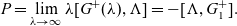
In this paper, we first present a class of non-local reverse-space matrix NLS equations by making a specific group of non-local reductions and then analyse their inverse scattering transforms and soliton solutions, based on associated Riemann–Hilbert problems. One example with two components is
 \begin{equation} \left\{ \begin{array} {l} ip_{1,t}(x,t)=p_{1,xx}(x,t)-2[\gamma_1p_1(x,t)p_1^*(-x,t)+\gamma _2 p_2(x,t)p_2^*(-x,t)]p_1(x,t), \\ \\[-7pt] ip_{2,t}(x,t)=p_{2,xx}(x,t)-2[\gamma _1p_1(x,t)p_1^*(-x,t)+\gamma _2 p_2(x,t)p_2^*(-x,t)]p_2(x,t), \end{array} \right. \end{equation}
where
 $\gamma _1$
and
$\gamma _1$
and
 $\gamma_2$
are arbitrary non-zero real constants.
$\gamma_2$
are arbitrary non-zero real constants.
The rest of the paper is organised as follows. In Section 2, within the zero curvature formulation, we recall the Ablowitz–Kaup–Newell–Segur (AKNS) integrable hierarchy with matrix potentials, based on an arbitrary-order matrix spectral problem suited for the Riemann–Hilbert theory, and conduct a group of non-local reductions to generate non-local reverse-space matrix NLS equations. In Section 3, we build the inverse scattering transforms by formulating Riemann–Hilbert problems associated with a kind of arbitrary-order matrix spectral problems. In Section 4, we compute soliton solutions to the obtained non-local reverse-space matrix NLS equations from the reflectionless transforms, that is, the special associated Riemann–Hilbert problems on the real axis where an identity jump matrix is taken. The conclusion is given in the last section, together with a few concluding remarks.
2 Non-local reverse-space matrix NLS equations
2.1 Matrix AKNS hierarchy
Let m and
 $n \ge 1 $
be two arbitrary integers, and
$n \ge 1 $
be two arbitrary integers, and
 $\alpha _1$
and
$\alpha _1$
and
 $\alpha_2$
are different arbitrary real constants. We focus on the following matrix spectral problem:
$\alpha_2$
are different arbitrary real constants. We focus on the following matrix spectral problem:
 \begin{equation} -i\phi_x =U\phi=U(p,q;\lambda)\phi,\ U=\left[\begin{array}{c@{\quad}c}\alpha _1 \lambda I_m & p\\ \\[-7pt] q& \alpha _2 \lambda I_n\end{array} \right],\end{equation}
where
 $\lambda $
is a spectral parameter, and p and q are two matrix potentials:
$\lambda $
is a spectral parameter, and p and q are two matrix potentials:
 \begin{equation}p=(p_{jl})_{m\times n},\ q=(q_{lj})_{n\times m}.\end{equation}
When
 $m=1$
, that is, p and q are vectors, (2.1) gives a matrix spectral problem with vector potentials [Reference Ma and Zhou37]. When there is only one pair of non-zero potentials
$m=1$
, that is, p and q are vectors, (2.1) gives a matrix spectral problem with vector potentials [Reference Ma and Zhou37]. When there is only one pair of non-zero potentials
 $p_{jl},q_{lj}$
, (2.1) becomes the standard AKNS spectral problem [Reference Ablowitz, Kaup, Newell and Segur1]. On account of these, we call (2.1) a matrix AKNS matrix spectral problem, and its associated hierarchy, a matrix AKNS integrable hierarchy. Because of the existence of a multiple eigenvalue of
$p_{jl},q_{lj}$
, (2.1) becomes the standard AKNS spectral problem [Reference Ablowitz, Kaup, Newell and Segur1]. On account of these, we call (2.1) a matrix AKNS matrix spectral problem, and its associated hierarchy, a matrix AKNS integrable hierarchy. Because of the existence of a multiple eigenvalue of
 $ \frac {\partial U}{\partial \lambda }$
, we have a degenerate matrix spectral problem in (2.1).
$ \frac {\partial U}{\partial \lambda }$
, we have a degenerate matrix spectral problem in (2.1).
To construct an associated matrix AKNS integrable hierarchy, as usual, we begin with the stationary zero curvature equation:
 \begin{equation}W_x=i[U,W],\end{equation}
corresponding to (2.1). We search for a solution W of the form:
 \begin{equation}W=\left[\begin{array}{c@{\quad}c}a&b \\c&d\end{array}\right], \end{equation}
where a, b, c and d are
 $m\times m$
,
$m\times m$
,
 $m\times n$
,
$m\times n$
,
 $n\times m$
and
$n\times m$
and
 $n\times n$
matrices, respectively. Obviously, the stationary zero curvature equation (2.3) equivalently presents
$n\times n$
matrices, respectively. Obviously, the stationary zero curvature equation (2.3) equivalently presents
 \begin{equation}\left\{\begin{array} {l}a_x=i(pc-bq),\\ \\[-7pt] b_x=i(\alpha \lambda b+pd-ap), \\ \\[-7pt] c_x=i(-\alpha \lambda c+qa-dq), \\ \\[-7pt] d_x=i(qb-cp), \end{array} \right.\end{equation}
where
 $\alpha =\alpha _1-\alpha _2$
. We take W as a formal series:
$\alpha =\alpha _1-\alpha _2$
. We take W as a formal series:
 \begin{equation}W=\left[\begin{array}{c@{\quad}c}a&b \\ \\[-7pt]c&d\end{array}\right]=\sum_{s=0}^\infty W_s\lambda^{-s},\ W_s=W_s(p,q)=\left[\begin{array}{c@{\quad}c}a^{[s]} &b^{[s]} \\ \\[-7pt]c^{[s]}&d^{[s]}\end{array}\right] ,\ s\ge 0,\end{equation}
and then, the system (2.5) exactly engenders the following recursion relations:
 \begin{align}b^{[0]}=0, \ c^{[0]}=0,\ a^{[0]}_x=0,\ d^{[0]}_x=0,\end{align}
 \begin{align}b^{[s+1]}= \displaystyle \frac 1{\alpha }( -i b^{[s]}_x - pd^{[s]} + a^{[s]}p),\ s\ge 0,\end{align}
 \begin{align}c^{[s+1]}=\displaystyle \frac 1{\alpha }( i c^{[s]}_x + qa^{[s]} - d^{[s]}q),\ s\ge 0,\end{align}
 \begin{align}a^{[s]}_x=i(pc^{[s]}-b^{[s]}q),\ d_x^{[s]}=i(qb^{[s]}-c^{[s]}p), \ s\ge 1 .\\[5pt] \nonumber\end{align}
Let us now fix the initial values:
 \begin{equation}a^{[0]}=\beta _1 I_m ,\ d^{[0]}=\beta _2 I_n,\end{equation}
where
 $\beta_1$
and
$\beta_1$
and
 $\beta_2$
are arbitrary but different real constants, and take zero constants of integration in (2.7d), which says that we require
$\beta_2$
are arbitrary but different real constants, and take zero constants of integration in (2.7d), which says that we require
 \begin{equation} W_s|_{p,q=0}=0,\ s\geq 1.\end{equation}
In this way, with
 $a^{[0]}$
and
$a^{[0]}$
and
 $ d^{[0]}$
given by (2.8), all matrices
$ d^{[0]}$
given by (2.8), all matrices
 $W_s ,\ s\ge 1$
, defined recursively, are uniquely determined. For example, a direct computation, based on (2.1), generates that
$W_s ,\ s\ge 1$
, defined recursively, are uniquely determined. For example, a direct computation, based on (2.1), generates that
 \begin{align}b^{[1]}=\dfrac \beta \alpha p,\ c^{[1]}=\dfrac{\beta}{\alpha} q,\ a^{[1]}=0,\ d^{[1]}=0; \end{align}
 \begin{align} b^{[2]}=-\dfrac{\beta}{\alpha ^2 }i p_{x},\ c^{[2]}=\dfrac{\beta }{\alpha ^2 }iq_{x},\ a^{[2]}=-\dfrac{\beta }{\alpha ^2 } pq,\ d^{[2]}=\dfrac{\beta }{\alpha ^2 }qp;\end{align}
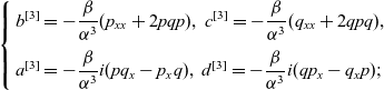 \begin{align}\left \{ \begin{array}{l}\displaystyle b^{[3]}=-\dfrac{\beta }{\alpha ^3 }(p_{xx}+2pq p),\ c^{[3]}=-\dfrac{\beta }{\alpha ^3 }(q_{xx}+2 q p q),\\ \\[-7pt]\displaystyle a^{[3]}=-\dfrac{\beta }{\alpha ^3 }i( pq_{x}-p_{x}q),\ d^{[3]}=-\dfrac{\beta }{\alpha ^3 }i(qp_{x} -q_{x}p );\end{array}\right.\end{align}
 \begin{align}\left\{\begin{array}{l}\displaystyle b^{[4]}=\dfrac{\beta}{\alpha ^4}i(p_{xxx}+3 pq p_{x} +3 p_{x} q p),\\ \\[-7pt]\displaystyle c^{[4]}=-\dfrac \beta {\alpha ^4 }i(q_{xxx}+3 q_x pq + 3q p q_{x}),\\ \\[-7pt]\displaystyle a^{[4]}=\dfrac \beta {\alpha ^4 }[3(pq )^2+p q_{xx} - p_{x}q_{x} + p_{xx} q],\\ \\[-7pt]\displaystyle d^{[4]}=-\dfrac \beta {\alpha ^4 }[3(q p)^2+q p_{xx} - q_{x} p_{x} + q_{xx}p ];\end{array}\right.\\ \nonumber\end{align}
where
 $\beta=\beta_1-\beta_2$
. Using (2.7d), we can derive, from (2.7b) and (2.7c), a recursion relation for
$\beta=\beta_1-\beta_2$
. Using (2.7d), we can derive, from (2.7b) and (2.7c), a recursion relation for
 $b^{[s]}$
and
$b^{[s]}$
and
 $c^{[s]}$
:
$c^{[s]}$
:
 \begin{equation} \left[ \begin{array}{c}c^{[s+1]}\\ \\[-7pt] b^{[s+1]}\end{array}\right]=\Psi \left[ \begin{array}{c}c^{[s]} \\ \\[-7pt] b^{[s]}\end{array}\right],\ s\ge 1,\end{equation}
where
 $\Psi $
is a matrix operator:
$\Psi $
is a matrix operator:
 \begin{equation}\Psi =\frac{i}{\alpha }\mbox{$ \left[\begin{array}{c@{\quad}c}{{(\partial_x + q \partial_x ^{-1}(p\, \cdot ) + [\partial_x^{-1}(\cdot \, p )] q )}} & {{- q\partial_x^{-1}(\cdot \, q) - [\partial_x^{-1}(q\, \cdot )]q}} \\ \\[-7pt]{{ p \partial_x ^{-1}(\cdot \, p) +[\partial_x^{-1}(p\, \cdot )] p }} &{{-\partial_x - p \partial_x^{-1}(q\, \cdot ) -[\partial_x^{-1}(\cdot \, q)]p } } \end{array}\right]$}.\end{equation}
The matrix AKNS integrable hierarchy is associated with the following temporal matrix spectral problems:
 \begin{equation}-i\phi_t=V^{[r]}\phi=V^{[r]}(p,q;\lambda)\phi , \ V^{[r]} =\sum_{s=0}^r W_m\lambda ^{r-s} ,\ r\ge 0.\end{equation}
The compatibility conditions of the two matrix spectral problems (2.1) and (2.13), that is, the zero curvature equations:
 \begin{equation}U_t-V^{[r]}_x+i[U,V^{[r]}]=0,\ r\ge 0, \end{equation}
yield the so-called matrix AKNS integrable hierarchy:
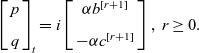 \begin{equation}\left [\begin{array}{l}p \\ \\[-7pt] q\end{array}\right] _{t }=i\left[\begin{array}{c}\alpha b^{[r+1]} \\ \\[-7pt]-\alpha c^{[r+1]}\end{array}\right],\ r\ge 0.\end{equation}
The first non-linear integrable system in this hierarchy gives us the standard matrix NLS equations:
 \begin{equation}\displaystyle p_{t }=-\frac{\beta}{\alpha ^2 }i (p_{xx}+2 p q p) ,\ \displaystyle q_{t }=\frac{\beta }{\alpha ^2 }i (q_{xx}+2 qpq ).\end{equation}
When
 $m=1$
and
$m=1$
and
 $n=2$
, under a special kind of symmetric reductions, the matrix NLS equations (2.16) can be reduced to the Manokov system [Reference Manakov39], for which a decomposition into finite-dimensional integrable Hamiltonian systems was made in [Reference Chen and Zhou8].
$n=2$
, under a special kind of symmetric reductions, the matrix NLS equations (2.16) can be reduced to the Manokov system [Reference Manakov39], for which a decomposition into finite-dimensional integrable Hamiltonian systems was made in [Reference Chen and Zhou8].
2.2 Non-local reverse-space matrix NLS equations
Let us now take a specific group of non-local reductions for the spectral matrix:
 \begin{equation}U^\dagger (-x,t,-\lambda ^*)=-C U(x,t,\lambda )C^{-1}, \ C=\left[ \begin{array} {c@{\quad}c} \Sigma_1 & 0 \\ \\[-7pt] 0 & \Sigma _2 \end{array} \right ], \ \Sigma_i ^\dagger = \Sigma_i,\ i=1,2,\end{equation}
which is equivalent to
 \begin{equation}P^\dagger (-x,t)=-CP(x,t)C^{-1}.\end{equation}
Henceforth,
 $\dagger $
stands for the Hermitian transpose,
$\dagger $
stands for the Hermitian transpose,
 $ * $
denotes the complex conjugate,
$ * $
denotes the complex conjugate,
 $\Sigma _{1,2}$
are two constant invertible Hermitian matrices, and for brevity, we adopt
$\Sigma _{1,2}$
are two constant invertible Hermitian matrices, and for brevity, we adopt
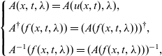 \begin{equation}\left\{ \begin{array}{l} A(x,t,\lambda )=A(u(x,t),\lambda), \\ \\[-7pt] A^\dagger (f(x,t,\lambda) )=(A(f(x,t,\lambda) ))^\dagger,\\ \\[-7pt] A^{-1}(f(x,t,\lambda) ) = (A( f(x,t,\lambda ) ))^{-1}, \end{array}\right. \end{equation}
for a matrix A and a function f.
The matrix spectral problems of the matrix NLS equations (2.16) are given as follows:
 \begin{equation}-i\phi_x=U \phi=U(p,q;\lambda)\phi, \ -i\phi_t=V^{[2]} \phi=V^{[2]}(p,q;\lambda)\phi.\end{equation}
The involved Lax pair reads
 \begin{equation}U=\lambda \Lambda +P,\ V^{[2]}= \lambda ^2 \Omega + Q,\end{equation}
where
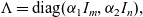 $\Lambda =\textrm{diag}(\alpha _1 I_m,\alpha _2I_n),$
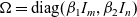 $ \Omega =\textrm{diag}(\beta _1 I_m,\beta _2 I_n)$
, and
$ \Omega =\textrm{diag}(\beta _1 I_m,\beta _2 I_n)$
, and
 \begin{equation}P= \left[\begin{array} {c@{\quad}c} 0 & p \\ \\[-7pt] q& 0\end{array} \right] ,\ Q=\left[\begin{array} {c@{\quad}c} a^{[1]}\lambda +a^{[2]} & b^{[1]}\lambda +b^{[2]} \\ \\[-7pt] c^{[1]}\lambda +c^{[2]} & d^{[1]}\lambda +d^{[2]}\end{array} \right]=\frac \beta {\alpha } \lambda\left[ \begin{array} {c@{\quad}c}0 & p \\ \\[-7pt] q& 0\end{array} \right]-\frac \beta {\alpha ^2 }\left[ \begin{array} {c@{\quad}c}pq & ip_x \\ \\[-7pt] -i q_x& -qp\end{array} \right].\end{equation}
In the above matrices P and Q, p and q are defined by (2.2), and
 $a^{[s]},b^{[s]},c^{[s]},d^{[s]}$
,
$a^{[s]},b^{[s]},c^{[s]},d^{[s]}$
,
 $ 1\le s\le 2$
, are determined in (2.10).
$ 1\le s\le 2$
, are determined in (2.10).
Based on (2.18), we arrive at
 \begin{equation} q(x,t)=-\Sigma _2^{-1} p^\dagger (-x,t) \Sigma_1 .\end{equation}
The vector function c in (2.5) under such a non-local reduction could be taken as:
 \begin{equation} c (x,t,\lambda ) = \Sigma _2 ^{-1} b^\dagger (-x,t,-\lambda ^*) \Sigma _1 .\end{equation}
It is easy to see that those non-local reduction relations ensure that
 \begin{equation} a^\dagger (-x,t,-\lambda ^*)=\Sigma_1 a(x,t,\lambda )\Sigma_1 ^{-1},\ d^\dagger (-x,t,-\lambda ^*)= \Sigma_2 d(x,t,\lambda )\Sigma _2 ^{-1}, \end{equation}
where a and d satisfy (2.5). For instance, under (2.23) and (2.24), we can compute that
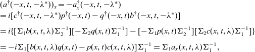 \begin{equation*}\begin{array} { l}(a ^\dagger (-x,t,-\lambda ^*))_x= -a_x^\dagger (-x,t,-\lambda ^*)\\= i[ c^\dagger (-x,t,-\lambda ^*)p^\dagger (-x,t) - q^\dagger (-x,t) b^\dagger (-x,t,-\lambda ^*) ]\\ \\[-7pt] = i\{ [ \Sigma_1 b (x,t,\lambda ) \Sigma _2 ^{-1} ][ -\Sigma _2 q (x,t)\Sigma _1^{-1} ] -[ -\Sigma _1 p(x,t)\Sigma _2 ^{-1}] [ \Sigma_2 c(x,t,\lambda )\Sigma _1 ^{-1} ] \}\\ \\[-7pt] =- i\Sigma _1 [ b(x,t,\lambda )q(x,t) - p(x,t)c(x,t,\lambda ) ] \Sigma _1^{-1} = \Sigma _1 a_x(x,t,\lambda) \Sigma _1 ^{-1} ,\end{array}\end{equation*}
from which the first relation in (2.25) follows. Furthermore, by using the Laurent expansions for a,b,c and d, we can get
 \begin{equation}\left\{ \begin{array} {l}(a^{[s]})^\dagger (-x,t)=(-1)^{s}\Sigma _1 a^{[s]}(x,t)\Sigma _1 ^{-1},\\ \\[-7pt] (b^{[s]})^{\dagger }(-x,t)= (-1)^{s} \Sigma_2 c^{[s]}(x,t)\Sigma _1 ^{-1},\\ \\[-7pt] (d^{[s]})^\dagger (-x,t)=(-1)^{s}\Sigma_2 d^{[s]}(x,t)\Sigma _2 ^{-1}, \end{array} \right.\end{equation}
where
 $s\ge 0$
. It then follows that
$s\ge 0$
. It then follows that
 \begin{equation}(V^{[2]})^\dagger (-x,t,-\lambda ^*) = C V^{[2]}(x,t,\lambda ) C^{-1},\ Q^\dagger (-x,t,- \lambda ^*) = C Q (x,t, \lambda )C^{-1},\end{equation}
where
 $V^{[2]}$
and Q are defined in (2.21) and (2.22), respectively.
$V^{[2]}$
and Q are defined in (2.21) and (2.22), respectively.
The above analysis guarantees that the non-local reduction (2.18) does not require any new condition for the compatibility of the spatial and temporal matrix spectral problems in (2.20). Therefore, the standard matrix NLS equations (2.16) are reduced to the following nonlocal reverse-space matrix NLS equations:
 \begin{equation} i p_{t}(x,t)=\frac \beta {\alpha ^2} [p_{xx}(x,t)- 2 p(x,t) \Sigma _2 ^{-1} p ^\dagger(-x,t)\Sigma _1p(x,t)], \end{equation}
where
 $\Sigma _1$
and
$\Sigma _1$
and
 $\Sigma _2$
are two arbitrary invertible Hermitian matrices.
$\Sigma _2$
are two arbitrary invertible Hermitian matrices.
When
 $m=n=1$
, we can get two well-known scalar examples [Reference Ablowitz and Musslimani3]:
$m=n=1$
, we can get two well-known scalar examples [Reference Ablowitz and Musslimani3]:
 \begin{equation}i p_t(x,t)=p_{xx}(x,t)-2\sigma p^2(x,t)p^*(-x,t), \ \sigma=\mp 1. \end{equation}
When
 $m=1$
and
$m=1$
and
 $n=2$
, we can obtain a system of non-local reverse-space two-component NLS equations (1.8).
$n=2$
, we can obtain a system of non-local reverse-space two-component NLS equations (1.8).
3 Inverse scattering transforms
3.1 Distribution of eigenvalues
We consider the non-local reduction case and so q is defined by (2.23). We are going to analyse the scattering and inverse scattering transforms for the non-local reverse-space matrix NLS equations (2.28) by the Riemann–Hilbert approach (see, e.g., [Reference Doktorov and Leble9, Reference Gerdjikov, Mladenov and Hirshfeld14, Reference Novikov, Manakov, Pitaevskii and Zakharov42]). The results will prepare the essential foundation for soliton solutions in the following section.
Assume that all the potentials sufficiently rapidly vanish when
 $x\to \pm \infty$
or
$x\to \pm \infty$
or
 $t\to \pm \infty$
. For the matrix spectral problems in (2.20), we can impose the asymptotic behaviour:
$t\to \pm \infty$
. For the matrix spectral problems in (2.20), we can impose the asymptotic behaviour:
 $\phi \sim \textrm{e}^{i\lambda \Lambda x+ i \lambda ^2 \Omega t}$
, when
$\phi \sim \textrm{e}^{i\lambda \Lambda x+ i \lambda ^2 \Omega t}$
, when
 $x,t\to \pm \infty$
. Therefore, if we take the variable transformation:
$x,t\to \pm \infty$
. Therefore, if we take the variable transformation:
 \begin{equation}\phi =\psi E_g,\ E_g=\textrm{e}^{i\lambda \Lambda x+ i \lambda ^2\Omega t},\nonumber\end{equation}
then we can have the canonical asymptotic conditions:
 $\psi \to I_{m+n}, \ \textrm{when}\ x,t \to \infty\ \textrm{or}\ -\infty.$
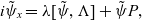
The equivalent pair of matrix spectral problems to (2.20) reads
$\psi \to I_{m+n}, \ \textrm{when}\ x,t \to \infty\ \textrm{or}\ -\infty.$
The equivalent pair of matrix spectral problems to (2.20) reads
 \begin{equation} \psi _x = i\lambda [\Lambda , \psi ] + \check{P} \psi , \ \check P=iP , \end{equation}
 \begin{align}\psi_t = i\lambda ^2[\Omega ,\psi ] + \check Q \psi, \ \check Q =iQ.\\[-7pt] \nonumber\end{align}
Applying a generalised Liouville’s formula [Reference Ma, Yong, Qin, Gu and Zhou34], we can obtain
 \begin{equation}\det \psi =1,\end{equation}
because
 $(\det \psi )_x=0$
due to
$(\det \psi )_x=0$
due to
 $\textrm{tr}\ \check P=\textrm{tr}\ \check Q=0$
.
$\textrm{tr}\ \check P=\textrm{tr}\ \check Q=0$
.
Recall that the adjoint equation of the x-part of (2.20) and the adjoint equation of (3.1) are given by:
 \begin{equation}i \tilde \phi _x = \tilde \phi U ,\end{equation}
and
 \begin{equation}i \tilde \psi _x = \lambda [\tilde \psi ,\Lambda ] +\tilde \psi P ,\end{equation}
respectively. Obviously, there exist the links:
 $\tilde \phi =\phi ^{-1}$
and
$\tilde \phi =\phi ^{-1}$
and
 $\tilde \psi=\psi ^{-1}$
. Each pair of adjoint matrix spectral problems and equivalent adjoint matrix spectral problems do not create any new condition, either, except the non-local reverse-space matrix NLS equations (2.28).
$\tilde \psi=\psi ^{-1}$
. Each pair of adjoint matrix spectral problems and equivalent adjoint matrix spectral problems do not create any new condition, either, except the non-local reverse-space matrix NLS equations (2.28).
Let
 $\psi(\lambda ) $
be a matrix eigenfunction of the spatial spectral problem (3.1) associated with an eigenvalue
$\psi(\lambda ) $
be a matrix eigenfunction of the spatial spectral problem (3.1) associated with an eigenvalue
 $\lambda$
. It is easy to see that
$\lambda$
. It is easy to see that
 $C\psi^{-1}(x,t, \lambda )$
is a matrix adjoint eigenfunction associated with the same eigenvalue
$C\psi^{-1}(x,t, \lambda )$
is a matrix adjoint eigenfunction associated with the same eigenvalue
 $\lambda$
. Under the non-local reduction in (2.18), we have
$\lambda$
. Under the non-local reduction in (2.18), we have
 \begin{equation*}\begin{array} {l}i[ \psi ^\dagger (-x,t, - \lambda ^* ) C ]_x = i [ - {(\psi _x)^\dagger (-x,t, - \lambda ^* )} C ]\\ \\[-7pt] =- i\{ (-i)(-\lambda ) [\psi ^\dagger (-x,t,-\lambda ^*),\Lambda ]+ (-i) \psi ^\dagger (-x,t,-\lambda ^*) P^\dagger (-x,t) \}C\\ \\[-7pt] = \lambda [\psi ^\dagger (-x,t,-\lambda ^*),\Lambda ] C+\psi^\dagger (-x,t,-\lambda ^*)C [-C^{-1} P^\dagger (-x,t)C]\\ \\[-7pt] =\lambda [\psi ^\dagger (-x,t,-\lambda ^*)C,\Lambda ] +\psi^\dagger (-x,t,-\lambda ^*)C P(x,t).\end{array}\end{equation*}
Thus, the matrix
 \begin{equation}\tilde \psi (x,t, \lambda ) :=\psi ^\dagger (-x,t, - \lambda ^* ) C ,\end{equation}
presents another matrix adjoint eigenfunction associated with the same original eigenvalue
 $ \lambda $
. That is to say that
$ \lambda $
. That is to say that
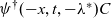 $ \psi ^\dagger (-x,t,- \lambda ^*) C $
solves the adjoint spectral problem (3.5).
$ \psi ^\dagger (-x,t,- \lambda ^*) C $
solves the adjoint spectral problem (3.5).
Finally, we observe the asymptotic conditions for the matrix eigenfunction
 $\psi$
, and see that by the uniqueness of solutions, we have
$\psi$
, and see that by the uniqueness of solutions, we have
 \begin{equation}\psi^\dagger (-x,t, -\lambda^* )=C\psi^{-1}(x,t,\lambda)C^{-1}, \end{equation}
when
 $\psi\to I_{m+n},\ x\ \textrm{or}\ t\to \infty\ \textrm{or}\ -\infty$
. This tells that if
$\psi\to I_{m+n},\ x\ \textrm{or}\ t\to \infty\ \textrm{or}\ -\infty$
. This tells that if
 $\lambda $
is an eigenvalue of (3.1) (or (3.5)), then
$\lambda $
is an eigenvalue of (3.1) (or (3.5)), then
 $-\lambda ^*$
will be another eigenvalue of (3.1) (or (3.5)), and there is the property (3.7) for the corresponding eigenfunction
$-\lambda ^*$
will be another eigenvalue of (3.1) (or (3.5)), and there is the property (3.7) for the corresponding eigenfunction
 $\psi$
.
$\psi$
.
3.2 Riemann–Hilbert problems
Let us now start to formulate a class of associated Riemann–Hilbert problems with the variable x. In order to clearly state the problems, we also make the assumptions:
 \begin{equation} \alpha=\alpha_1-\alpha _2 <0,\ \beta =\beta _1-\beta _2<0.\end{equation}
In the scattering problem, we first introduce the two matrix eigenfunctions
 $\psi^\pm (x,\lambda )$
of (3.1) with the asymptotic conditions:
$\psi^\pm (x,\lambda )$
of (3.1) with the asymptotic conditions:
 \begin{equation}\psi^{\pm} \to I_{m+n},\ \textrm{when}\ x \to \pm \infty,\end{equation}
respectively. It then follows from (3.3) that
 $\det \psi ^\pm =1$
for all
$\det \psi ^\pm =1$
for all
 $x\in \mathbb{R}$
. Because
$x\in \mathbb{R}$
. Because
 \begin{equation}\phi^{\pm} =\psi^{\pm}E, \ E=\textrm{e}^{i\lambda \Lambda x},\end{equation}
are both matrix eigenfunctions of (2.20), they must be linearly dependent, and as a result, one has
 \begin{equation}\psi^-E = \psi^+ES(\lambda ), \ \lambda \in \mathbb{R} ,\end{equation}
where
 $S(\lambda )$
is the corresponding scattering matrix. Note that
$S(\lambda )$
is the corresponding scattering matrix. Note that
 $\det S(\lambda )=1$
, thanks to
$\det S(\lambda )=1$
, thanks to
 $\det \psi ^\pm=1$
.
$\det \psi ^\pm=1$
.
Through the method of variation in parameters, we can transform the x-part of (2.20) into the following Volterra integral equations for
 $\psi^{\pm}$
[Reference Novikov, Manakov, Pitaevskii and Zakharov42]:
$\psi^{\pm}$
[Reference Novikov, Manakov, Pitaevskii and Zakharov42]:
 \begin{align}& \psi ^-(\lambda ,x) = I _{m+n}+\int_{-\infty}^x\textrm{e}^{i\lambda \Lambda (x-y )}\check P(y)\psi ^-(\lambda ,y)\textrm{e}^{i\lambda \Lambda (y-x)}\,dy,\end{align}
 \begin{align}& \psi^+(\lambda ,x) = I _{m+n}-\int_x^{\infty}\textrm{e}^{i\lambda \Lambda (x-y)}\check P (y)\psi ^+(\lambda ,y)\textrm{e}^{i\lambda \Lambda (y-x)}\,dy,\\[-7pt] \nonumber\end{align}
where the asymptotic conditions (3.9) have been imposed. Now, the theory of Volterra integral equations tells that by the Neumann series [Reference Hildebrand18], we can show that the eigenfunctions
 $\psi ^\pm$
exist and allow analytic continuations off the real axis
$\psi ^\pm$
exist and allow analytic continuations off the real axis
 $\lambda\in \mathbb{R}$
provided that the integrals on their right-hand sides converge (see, e.g., [Reference Ablowitz, Prinari and Trubatch6]). From the diagonal form of
$\lambda\in \mathbb{R}$
provided that the integrals on their right-hand sides converge (see, e.g., [Reference Ablowitz, Prinari and Trubatch6]). From the diagonal form of
 $\Lambda$
and the first assumption in (3.8), we can see that the integral equation for the first m columns of
$\Lambda$
and the first assumption in (3.8), we can see that the integral equation for the first m columns of
 $\psi ^-$
contains only the exponential factor
$\psi ^-$
contains only the exponential factor
 $\textrm{e}^{-i\alpha \lambda (x-y)}$
, which decays because of
$\textrm{e}^{-i\alpha \lambda (x-y)}$
, which decays because of
 $y< x$
in the integral, if
$y< x$
in the integral, if
 $\lambda $
takes values in the upper half-plane
$\lambda $
takes values in the upper half-plane
 $\mathbb{C}^+$
, and the integral equation for the last n columns of
$\mathbb{C}^+$
, and the integral equation for the last n columns of
 $\psi^+$
contains only the exponential factor
$\psi^+$
contains only the exponential factor
 $\textrm{e}^{i \alpha \lambda (x-y)}$
, which also decays because of
$\textrm{e}^{i \alpha \lambda (x-y)}$
, which also decays because of
 $y> x$
in the integral, when
$y> x$
in the integral, when
 $\lambda $
takes values in the upper half-plane
$\lambda $
takes values in the upper half-plane
 $\mathbb{C}^+$
. Therefore, we see that these
$\mathbb{C}^+$
. Therefore, we see that these
 $m+n$
columns are analytic in the upper half-plane
$m+n$
columns are analytic in the upper half-plane
 $\mathbb{C}^+$
and continuous in the closed upper half-plane
$\mathbb{C}^+$
and continuous in the closed upper half-plane
 $\mathbb{\bar C}^+$
. In a similar manner, we can know that the last n columns of
$\mathbb{\bar C}^+$
. In a similar manner, we can know that the last n columns of
 $\psi ^-$
and the first m columns of
$\psi ^-$
and the first m columns of
 $\psi^+$
are analytic in the lower half-plane
$\psi^+$
are analytic in the lower half-plane
 $ \mathbb{C}^-$
and continuous in the closed lower half-plane
$ \mathbb{C}^-$
and continuous in the closed lower half-plane
 $\mathbb{\bar C}^-$
.
$\mathbb{\bar C}^-$
.
In what follows, we give a detailed proof for the above statements. Let us express
 \begin{equation}\psi^{\pm}=(\psi^{\pm}_1,\psi^{\pm}_2,\cdots,\psi^{\pm}_{m+n}),\end{equation}
that is,
 $\psi^{\pm}_j$
denotes the jth column of
$\psi^{\pm}_j$
denotes the jth column of
 $\phi^{\pm}$
(
$\phi^{\pm}$
(
 $1\le j\le m+n$
). We would like to prove that
$1\le j\le m+n$
). We would like to prove that
 $\psi^{-}_j$
,
$\psi^{-}_j$
,
 $1\le j\le m$
, and
$1\le j\le m$
, and
 $\psi^{+}_j$
,
$\psi^{+}_j$
,
 $m+1\le j\le m+n$
, are analytic at
$m+1\le j\le m+n$
, are analytic at
 $\lambda \in \mathbb{C}^+$
and continuous at
$\lambda \in \mathbb{C}^+$
and continuous at
 $\lambda \in \mathbb{\bar C}^+$
; and
$\lambda \in \mathbb{\bar C}^+$
; and
 $\psi^{+}_j$
,
$\psi^{+}_j$
,
 $1\le j\le m$
, and
$1\le j\le m$
, and
 $\psi^{-}_j$
,
$\psi^{-}_j$
,
 $m+1\le j\le m+n$
, are analytic at
$m+1\le j\le m+n$
, are analytic at
 $\lambda \in \mathbb{C}^-$
and continuous at
$\lambda \in \mathbb{C}^-$
and continuous at
 $\lambda \in \mathbb{\bar C}^-$
. We only to prove the result for
$\lambda \in \mathbb{\bar C}^-$
. We only to prove the result for
 $\psi^{-}_j$
,
$\psi^{-}_j$
,
 $1\le j\le m$
, and the proofs for the other eigenfunctions follow analogously.
$1\le j\le m$
, and the proofs for the other eigenfunctions follow analogously.
It is easy to obtain from the Volterra integral equation (3.12) that
 \begin{equation}\psi^-_j(\lambda ,x)= \textrm{e}_j + \int_{-\infty}^x R_1 (\lambda ,x,y) \psi^-_j(\lambda ,y)\, dy, \ 1\le j\le m, \end{equation}
and
 \begin{equation}\psi^-_j(\lambda ,x)= \textrm{e}_j + \int_{-\infty}^x R_2 (\lambda ,x,y) \psi^-_j(\lambda ,y)\, dy, \ m+1\le j\le m+n, \end{equation}
where the
 $\textrm{e}_i$
are standard basis vectors of
$\textrm{e}_i$
are standard basis vectors of
 $\mathbb{R}^{m+n}$
and the matrices
$\mathbb{R}^{m+n}$
and the matrices
 $R_1$
and
$R_1$
and
 $R_2$
are defined by:
$R_2$
are defined by:
 \begin{equation} R_1(\lambda ,x,y)=i\left[\begin{array} {c@{\quad}c} 0& p (y) \\ \\[-7pt] \textrm{e}^{-i\alpha \lambda (x-y) }q(y) & 0 \end{array} \right],\ R_2(\lambda ,x,y)=i\left[\begin{array} {c@{\quad}c} 0& \textrm{e}^{i\alpha \lambda (x-y) }p(y) \\ \\[-7pt] q(y) & 0 \end{array} \right].\end{equation}
Let us prove that for each
 $1\le j\le m$
, the solution to (3.15) is determined by the Neumann series:
$1\le j\le m$
, the solution to (3.15) is determined by the Neumann series:
 \begin{equation} \sum_{k=0} ^\infty \phi^-_{j,k}(\lambda ,x), \end{equation}
where
 \begin{align} \phi^-_{j,0}(\lambda ,x)=\textrm{e}_j,\ phi^-_{j,k+1}(\lambda ,x)= \int_{-\infty}^xR_1(\lambda, x,y)\phi^-_{j,k}(\lambda ,y)\, dy,\ k\ge 1. \end{align}
This will be true if we can prove that the Neumann series converges uniformly for
 $x\in \mathbb{R}$
and
$x\in \mathbb{R}$
and
 $\lambda \in \mathbb{\bar C}^+$
. By the mathematical induction, we can have
$\lambda \in \mathbb{\bar C}^+$
. By the mathematical induction, we can have
 \begin{equation}|\phi^-_{j,k}(\lambda ,x)|\le \frac 1 {k!} \Bigl( \int_{-\infty}^x \| P(y) \| dy \Bigr)^k,\ 1\le j\le m,\ k\ge 0,\end{equation}
for
 $x\in \mathbb{R}$
and
$x\in \mathbb{R}$
and
 $ \lambda \in \mathbb{\bar C}^+$
, where
$ \lambda \in \mathbb{\bar C}^+$
, where
 $|\cdot |$
denotes the Euclidean norm for vectors and
$|\cdot |$
denotes the Euclidean norm for vectors and
 $\|\cdot \|$
stands for the Frobenius norm for square matrices. By the Weierstrass M-test, this estimation guarantees that
$\|\cdot \|$
stands for the Frobenius norm for square matrices. By the Weierstrass M-test, this estimation guarantees that
 \begin{equation} \phi^-_j(\lambda ,x)=\sum_{k=0} ^\infty \phi^-_{j,k}(\lambda ,x), \ 1\le j\le m,\end{equation}
uniformly converges for
 $ \lambda \in \mathbb{\bar C}^+$
and
$ \lambda \in \mathbb{\bar C}^+$
and
 $x\in \mathbb{R}$
, and all
$x\in \mathbb{R}$
, and all
 $\phi^-_j(\lambda ,x)$
,
$\phi^-_j(\lambda ,x)$
,
 $1\le j\le m$
, are continuous with respect to
$1\le j\le m$
, are continuous with respect to
 $\lambda$
in
$\lambda$
in
 $ \mathbb{\bar C}^+$
, since so are all
$ \mathbb{\bar C}^+$
, since so are all
 $\phi^-_{j,k}(\lambda ,x)$
,
$\phi^-_{j,k}(\lambda ,x)$
,
 $1\le j\le m$
,
$1\le j\le m$
,
 $k\ge 0$
.
$k\ge 0$
.
Let us now consider the differentiability of
 $ \phi^-_j(\lambda ,x)$
,
$ \phi^-_j(\lambda ,x)$
,
 $1\le j\le m$
, with respect to
$1\le j\le m$
, with respect to
 $\lambda $
in
$\lambda $
in
 $ \mathbb{C}^+$
(similarly, we can prove the differentiability with respect to x in
$ \mathbb{C}^+$
(similarly, we can prove the differentiability with respect to x in
 $\mathbb{R}$
). Fix an integer
$\mathbb{R}$
). Fix an integer
 $1\le j\le m$
and a number
$1\le j\le m$
and a number
 $\mu $
in
$\mu $
in
 $ \mathbb{C}^+$
. Choose a disc
$ \mathbb{C}^+$
. Choose a disc
 $B_r(\mu )=\{\lambda \in \mathbb{C}\,|\, |\lambda -\mu |\le r \} $
with a radius
$B_r(\mu )=\{\lambda \in \mathbb{C}\,|\, |\lambda -\mu |\le r \} $
with a radius
 $r> 0$
such that
$r> 0$
such that
 $B_r(\mu )\subseteq \mathbb{C}^+$
, and then we can have a constant
$B_r(\mu )\subseteq \mathbb{C}^+$
, and then we can have a constant
 $C(r)>0$
such that
$C(r)>0$
such that
 $|\alpha x \textrm{e}^{-i \alpha \lambda x} | \le C(r)$
for
$|\alpha x \textrm{e}^{-i \alpha \lambda x} | \le C(r)$
for
 $\lambda \in B_r(\mu )$
and
$\lambda \in B_r(\mu )$
and
 $x\ge 0$
. We define the following Neumann series:
$x\ge 0$
. We define the following Neumann series:
 \begin{equation} \sum_{k=0}^\infty\phi^-_{j,\lambda,k}(\lambda ,x),\end{equation}
where
 $\phi^-_{j,\lambda,0}=0 $
and
$\phi^-_{j,\lambda,0}=0 $
and
 \begin{equation}\phi^-_{j,\lambda,k+1}(\lambda ,x)=\int_{-\infty}^x R_{1,\lambda }(\lambda ,x,y)\phi^-_{j,k}(\lambda ,y)\, dy+\int_{-\infty}^x R_1(\lambda ,x,y)\phi^-_{j,\lambda,k}(\lambda , y)\, dy,\ k\ge 0,\end{equation}
with the
 $\phi^-_{j,k}$
being given by (3.19) and
$\phi^-_{j,k}$
being given by (3.19) and
 $R_{1,\lambda }$
being defined by:
$R_{1,\lambda }$
being defined by:
 \begin{equation} R_{1,\lambda }(\lambda ,x,y)= \frac {\partial}{\partial \lambda }R_1(\lambda ,x,y)=\left [\begin{array} {c@{\quad}c}0& 0\\ \\[-7pt] \alpha (x-y)\textrm{e}^{-i\alpha \lambda (x-y)} q(y) & 0\end{array}\right].\end{equation}
We can readily verify by the mathematical induction that
 \begin{equation}|\phi^-_{j,\lambda,k}(\lambda ,x)|\le \frac 1 {k!} \Bigl\{\bigl[C(r)+1\bigr] \int_{-\infty}^x \| P(y) \| dy \Bigr\}^k,\ k\ge 0,\end{equation}
for
 $x\in \mathbb{R}$
and
$x\in \mathbb{R}$
and
 $ \lambda \in B_r(\mu )$
. Therefore, by the Weierstrass M-test, the Neumann series defined by (3.22) converges uniformly for
$ \lambda \in B_r(\mu )$
. Therefore, by the Weierstrass M-test, the Neumann series defined by (3.22) converges uniformly for
 $x\in \mathbb{R}$
and
$x\in \mathbb{R}$
and
 $ \lambda \in B_r(\mu)$
; and by the term-by-term differentiability theorem, it converges to the derivative of
$ \lambda \in B_r(\mu)$
; and by the term-by-term differentiability theorem, it converges to the derivative of
 $\phi^-_j$
with respect to
$\phi^-_j$
with respect to
 $\lambda$
, due to
$\lambda$
, due to
 $\psi^-_{j,\lambda,k}=\frac {\partial }{\partial \lambda }\phi^-_{j,k}$
,
$\psi^-_{j,\lambda,k}=\frac {\partial }{\partial \lambda }\phi^-_{j,k}$
,
 $k\ge 0$
. Therefore,
$k\ge 0$
. Therefore,
 $\phi^-_j$
is analytic at an arbitrarily fixed point
$\phi^-_j$
is analytic at an arbitrarily fixed point
 $\mu \in \mathbb{C}^+$
. It then follows that all
$\mu \in \mathbb{C}^+$
. It then follows that all
 $\phi^-_j$
,
$\phi^-_j$
,
 $1\le j\le m,$
are analytic with respect to
$1\le j\le m,$
are analytic with respect to
 $\lambda$
in
$\lambda$
in
 $ \mathbb{C}^+$
. The required proof is done.
$ \mathbb{C}^+$
. The required proof is done.
Based on the above analysis, we can then form the generalised matrix Jost solution
 $T^+$
as follows:
$T^+$
as follows:
 \begin{equation}T^+=T^+(x,\lambda) = (\psi^- _1,\cdots,\psi^- _m,\psi^+_ {m+1},\cdots,\psi^+_{m+n})= \psi^-H_1 + \psi^+ H_2 ,\end{equation}
which is analytic with respect to
 $\lambda$
in
$\lambda$
in
 $\mathbb{C}^+$
and continuous with respect to
$\mathbb{C}^+$
and continuous with respect to
 $\lambda$
in
$\lambda$
in
 $\mathbb{\bar C}^+$
. The generalised matrix Jost solution:
$\mathbb{\bar C}^+$
. The generalised matrix Jost solution:
 \begin{equation}(\psi^+_1 ,\cdots, \psi^+_m , \psi^-_{m+1} , \cdots, \psi^-_{m+n})=\psi^+H_1+\psi^-H_2\end{equation}
is analytic with respect to
 $\lambda $
in
$\lambda $
in
 $\mathbb{C}^-$
and continuous with respect to
$\mathbb{C}^-$
and continuous with respect to
 $\lambda$
in
$\lambda$
in
 $\mathbb{\bar C}^-$
. In the above definition, we have used
$\mathbb{\bar C}^-$
. In the above definition, we have used
 \begin{equation}H_1=\textrm{diag}(I_m,\underbrace{0,\cdots,0}_{n}\, ),\ H_2=\textrm{diag}(\underbrace{0,\cdots,0}_{m},I_n\,).\end{equation}
To construct the other generalised matrix Jost solution
 $T^-$
, we adopt the analytic counterpart of
$T^-$
, we adopt the analytic counterpart of
 $T^+$
in the lower half-plane
$T^+$
in the lower half-plane
 $\mathbb{C}^-$
, which can be generated from the adjoint counterparts of the matrix spectral problems. Note that the inverse matrices
$\mathbb{C}^-$
, which can be generated from the adjoint counterparts of the matrix spectral problems. Note that the inverse matrices
 $\tilde \phi ^{\pm}=(\phi ^\pm )^{-1}$
and
$\tilde \phi ^{\pm}=(\phi ^\pm )^{-1}$
and
 $\tilde \psi ^{\pm}=(\psi ^\pm )^{-1}$
solve those two adjoint equations, respectively. Then, stating
$\tilde \psi ^{\pm}=(\psi ^\pm )^{-1}$
solve those two adjoint equations, respectively. Then, stating
 $\tilde \psi^{\pm}$
as:
$\tilde \psi^{\pm}$
as:
 \begin{equation}\tilde \psi ^{\pm} =(\tilde \psi ^{\pm,1},\tilde \psi^{\pm,2} ,\cdots,\tilde\psi^{\pm,m+n})^T,\end{equation}
that is,
 $\tilde \psi ^{\pm,j}$
denotes the jth row of
$\tilde \psi ^{\pm,j}$
denotes the jth row of
 $\tilde \psi ^{\pm}$
(
$\tilde \psi ^{\pm}$
(
 $1\le j\le m+n$
), we can verify by similar arguments that we can form the generalised matrix Jost solution
$1\le j\le m+n$
), we can verify by similar arguments that we can form the generalised matrix Jost solution
 $T^-$
as the adjoint matrix solution of (3.5), that is,
$T^-$
as the adjoint matrix solution of (3.5), that is,
 \begin{equation}T^- =(\tilde \psi ^{-,1},\cdots, \tilde \psi ^{-,m},\tilde \psi ^{+,m+1},\cdots,\tilde \psi ^{+,m+n})^T = H_1\tilde \psi ^{-} + H_2\tilde \psi ^{+}=H_1(\psi^-)^{-1}+H_2(\psi ^+)^{-1},\end{equation}
which is analytic with respect to
 $ \lambda$
in
$ \lambda$
in
 $\mathbb{C}^-$
and continuous with respect to
$\mathbb{C}^-$
and continuous with respect to
 $\lambda$
in
$\lambda$
in
 $\mathbb{\bar C}^-$
, and the other generalised matrix Jost solution of (3.5):
$\mathbb{\bar C}^-$
, and the other generalised matrix Jost solution of (3.5):
 \begin{equation}(\tilde \psi ^{+,1},\cdots, \tilde \psi ^{+,m},\tilde \psi ^{-,m+1},\cdots,\tilde \psi ^{-,m+n})^T = H_1\tilde \psi ^{+} + H_2\tilde \psi ^{-} =H_1(\psi^+)^{-1} +H_2 (\psi^-)^{-1} ,\end{equation}
is analytic with respect to
 $ \lambda$
in
$ \lambda$
in
 $\mathbb{C}^+$
and continuous with respect to
$\mathbb{C}^+$
and continuous with respect to
 $\lambda$
in
$\lambda$
in
 $\mathbb{\bar C}^+$
.
$\mathbb{\bar C}^+$
.
Now we have finished the construction of the two generalised matrix Jost solutions,
 $T^+$
and
$T^+$
and
 $T^-$
. Directly from
$T^-$
. Directly from
 $\det \psi ^\pm =1$
and using the scattering relation (3.11) between
$\det \psi ^\pm =1$
and using the scattering relation (3.11) between
 $\psi ^+$
and
$\psi ^+$
and
 $\psi ^-$
, we arrive at
$\psi ^-$
, we arrive at
 \begin{equation} \lim _{x\to \infty} T^+(x,\lambda ) = \left [\begin{array} {c@{\quad}c} S_{11}(\lambda ) & 0 \\ \\[-7pt] 0 & I_n \end{array} \right] ,\ \lambda \in \mathbb{\bar C}^+, lim _{x\to -\infty} T^-(x,\lambda ) = \left [\begin{array} {c@{\quad}c} \hat S_{11}(\lambda ) & 0 \\ 0 & I_n \end{array} \right] ,\ \lambda \in \mathbb{\bar C}^- , \end{equation}
and
 \begin{equation}\det T^+(x,\lambda) = \det S_{11}(\lambda), \ \det T^-(x,\lambda) =\det \hat S _{11}(\lambda ),\end{equation}
where we split
 $S(\lambda )$
and
$S(\lambda )$
and
 $S^{-1}(\lambda )$
as follows:
$S^{-1}(\lambda )$
as follows:
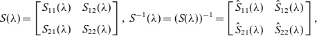 \begin{equation} S(\lambda ) =\left [ \begin{array} {c@{\quad}c} S_{11}(\lambda ) & S_{12} (\lambda )\\ \\[-7pt]S_{21}(\lambda )& S_{22} (\lambda ) \end{array} \right ],\ S^{-1}(\lambda ) =(S(\lambda ))^{-1}=\left[ \begin{array} {c@{\quad}c} \hat S _{11}(\lambda ) & \hat S_{12}(\lambda ) \\ \\[-7pt]\hat S_{21}(\lambda )& \hat S_{22}(\lambda )\end{array} \right],\end{equation}
 $S_{11},\hat S_{11}$
being
$S_{11},\hat S_{11}$
being
 $m\times m$
matrices,
$m\times m$
matrices,
 $S_{12},\hat S_{12}$
being
$S_{12},\hat S_{12}$
being
 $m\times n$
matrices,
$m\times n$
matrices,
 $S_{21},\hat S_{21}$
being
$S_{21},\hat S_{21}$
being
 $n\times m$
matrices and
$n\times m$
matrices and
 $S_{22},\hat S_{22}$
being
$S_{22},\hat S_{22}$
being
 $n\times n$
matrices. Based on the uniform convergence of the previous Neumann series, we know that
$n\times n$
matrices. Based on the uniform convergence of the previous Neumann series, we know that
 $S_{11}(\lambda )$
and
$S_{11}(\lambda )$
and
 $\hat S_{11}(\lambda )$
are analytic in
$\hat S_{11}(\lambda )$
are analytic in
 $ \mathbb{C}^+$
and
$ \mathbb{C}^+$
and
 $ \mathbb{C}^-$
, respectively.
$ \mathbb{C}^-$
, respectively.
In this way, we can introduce the following two unimodular generalised matrix Jost solutions:
 \begin{equation}\left \{ \begin{array} {l}G^+(x,\lambda ) =T^+(x,\lambda ) \left [\begin{array} {c@{\quad}c} S_{11}^{-1}(\lambda ) & 0 \\ \\[-7pt] 0 & I_n \end{array} \right],\quad \lambda \in \mathbb{\bar C}^+;\\[3pt] (G^-)^{-1}(x,\lambda ) = \left [\begin{array} {c@{\quad}c} \hat S^{-1}_{11}(\lambda ) & 0 \\ \\[-7pt] 0 & I_n \end{array} \right] T^-(x,\lambda),\ \lambda \in \mathbb{\bar C}^-.\end{array} \right.\end{equation}
Those two generalised matrix Jost solutions establish the required matrix Riemann–Hilbert problems on the real line for the non-local reverse-space matrix NLS equations (2.28):
 \begin{equation}G^+(x,\lambda ) = G^-(x,\lambda ) G_0(x,\lambda), \ \lambda \in \mathbb{R} ,\end{equation}
where the jump matrix
 $G_0$
is
$G_0$
is
 \begin{equation}G_0(x,\lambda) = E \left [\begin{array} {c@{\quad}c} \hat S^{-1}_{11}(\lambda ) & 0 \\ \\[-7pt] 0 & I_n \end{array} \right] \tilde S(\lambda ) \left [\begin{array} {c@{\quad}c} S_{11}^{-1}(\lambda ) & 0 \\ \\[-7pt] 0 & I_n \end{array} \right] E^{-1} ,\end{equation}
based on (3.11). In the jump matrix
 $G_0$
, the matrix
$G_0$
, the matrix
 $\tilde S(\lambda )$
has the factorisation:
$\tilde S(\lambda )$
has the factorisation:
 \begin{equation}\tilde S(\lambda )=(H_1 + H_2S(\lambda ))\ (H_1 + S^{-1}(\lambda )H_2),\end{equation}
which can be shown to be
 \begin{equation} \tilde S(\lambda )= \left[\begin{array} {c@{\quad}c} I_m & \hat S_{12} \\ \\[-7pt] S_{21} & I_n\end{array} \right]. \end{equation}
Following the Volterra integral equations (3.12) and (3.13), we can obtain the canonical normalisation conditions:
 \begin{equation}G^\pm (x,\lambda ) \to I_{m+n},\ \textrm{when}\ \lambda \in \mathbb{\bar C}^\pm \to \infty,\end{equation}
for the presented Riemann–Hilbert problems. From the property (3.7), we can also observe that
 \begin{equation}(G^+)^\dagger (-x,t,-\lambda ^*)=C (G^-)^{-1}(x,t,\lambda ) C^{-1},\end{equation}
and thus, the the jump matrix
 $G_0$
possesses the following involution property:
$G_0$
possesses the following involution property:
 \begin{equation}G_0^\dagger (-x,t,-\lambda ^*)=C G_0(x,t,\lambda ) C^{-1}. \end{equation}
3.3 Evolution of the scattering data
To complete the direct scattering transforms, let us take the derivative of (3.11) with time t and use the temporal matrix spectral problems:
 \begin{equation} \psi^\pm _t =i\lambda ^2 [\Omega ,\psi ^\pm] +\check Q \psi ^\pm.\end{equation}
It then follows that the scattering matrix S satisfies the following evolution law:
 \begin{equation} S_t = i\lambda ^2[\Omega ,S].\end{equation}
This tells the time evolution of the time-dependent scattering coefficients:
 \begin{equation} S_{12}=S_{12}(t,\lambda ) = S_{12}(0,\lambda ) \, \textrm{e}^{i\beta \lambda ^2 t},\ S_{21}=S_{21}(t,\lambda ) =S_{21}(0,\lambda ) \, \textrm{e}^{-i\beta \lambda ^2 t}, \end{equation}
and all other scattering coefficients are independent of the time variable t.
3.4 Gelfand–Levitan–Marchenko-type equations
To obtain Gelfand–Levitan–Marchenko-type integral equations to determine the generalised matrix Jost solutions, let us transform the associated Riemann–Hilbert problem (3.36) into
 \begin{equation} \left\{ \begin{array} {l}G^+-G^- =G^-v , \ v=G_0-I_{m+n},\ \textrm{on}\ \mathbb{R},\\ \\[-7pt] G^\pm \to I_{m+n}\ \textrm{as}\ \lambda \in \mathbb{\bar C} ^\pm \to \infty,\end{array}\right.\end{equation}
where the jump matrix
 $G_0$
is defined by (3.37) and (3.38).
$G_0$
is defined by (3.37) and (3.38).
Let
 $G(\lambda )=G ^\pm (\lambda )$
if
$G(\lambda )=G ^\pm (\lambda )$
if
 $\lambda \in \mathbb{C}^\pm$
. Assume that G has simple poles off
$\lambda \in \mathbb{C}^\pm$
. Assume that G has simple poles off
 $\mathbb{R}$
:
$\mathbb{R}$
:
 $\{ \mu _j\}_{j=1}^R$
, where R is an arbitrary integer. Define
$\{ \mu _j\}_{j=1}^R$
, where R is an arbitrary integer. Define
 \begin{equation} \tilde G^\pm (\lambda ) = G^\pm (\lambda )- \sum_{j=1}^R \frac {G_j } {\lambda -\mu _j},\ \lambda \in \mathbb{\bar C}^\pm ; \ \tilde G (\lambda ) =\tilde G^\pm (\lambda ) ,\ \lambda \in \mathbb{C}^\pm ,\end{equation}
where
 $ G_j$
is the residue of G at
$ G_j$
is the residue of G at
 $\lambda =\mu _j$
, that is,
$\lambda =\mu _j$
, that is,
 \begin{equation} G_j= \textrm{res}(G(\lambda),\lambda _j)= \lim_{\lambda \to \mu _j}(\lambda -\mu _j)G(\lambda ). \end{equation}
This tells that we have
 \begin{equation} \left\{ \begin{array} {l}\tilde G^+-\tilde G^- =G^+-G^-= G^-v , \ \textrm{on}\ \mathbb{R},\\\tilde G^\pm \to I_{m+n}\ \textrm{as}\ \lambda \in \mathbb{\bar C}^\pm \to \infty.\end{array}\right.\end{equation}
By applying the Sokhotski–Plemelj formula [Reference Gakhov12], we get the solution of (3.49):
 \begin{equation} \tilde G(\lambda ) = I_{m+n}+ \frac {1}{2\pi i} \int_{-\infty}^\infty \frac { (G^-v) (\xi )}{\xi -\lambda }\, d\xi.\end{equation}
Further taking the limit as
 $\lambda \to \mu _l $
yields
$\lambda \to \mu _l $
yields
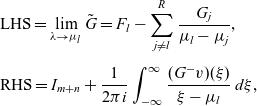 \begin{equation*}\begin{array}{l}\displaystyle \textrm{LHS}=\lim_{\lambda \to \mu _l} \tilde G =F_l -\sum_{j\ne l}^R \frac {G_j }{\mu _l-\mu _j} ,\\ \\[-6pt] \displaystyle \textrm{RHS}= I_{m+n}+\frac 1 {2\pi i}\int_{-\infty}^\infty \frac {(G^-v)(\xi ) }{\xi -\mu _l } \, d\xi ,\end{array}\end{equation*}
where
 \begin{equation} F_l=\lim_{\lambda \to \mu _l}\frac {(\lambda -\mu _l)G(\lambda )-G_l} {\lambda -\mu_l},\ 1\le l\le R,\end{equation}
and consequently, we see that the required Gelfand–Levitan–Marchenko-type integral equations are as follows:
 \begin{equation}I_{m+n}-F_l+\sum_{j\ne l}^R \frac {G_j }{\mu _l-\mu _j}+\frac 1 {2\pi i}\int_{-\infty}^\infty \frac {(G^-v)(\xi ) }{\xi -\mu _l } \, d\xi =0,\ 1\le l\le R.\end{equation}
All these equations are used to determine solutions to the associated Riemann–Hilbert problems and thus the generalised matrix Jost solutions. However, little was yet known about the existence and uniqueness of solutions. In the case of soliton solutions, a formulation of solutions, where eigenvalues could equal adjoint eigenvalues, will be presented for non-local integrable equations in the next section.
3.5 Recovery of the potential
To recover the potential matrix P from the generalised matrix Jost solutions, as usual, we make an asymptotic expansion:
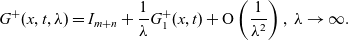 \begin{equation}G^+(x,t,\lambda ) = I_{m+n} +\frac{1}{\lambda}G^+_1(x,t) + \textrm{O}\left(\frac 1 {\lambda ^{2}}\right), \ \lambda\to \infty .\end{equation}
Then, plugging this asymptotic expansion into the matrix spectral problem (3.1) and comparing
 $\textrm{O}(1)$
terms generates
$\textrm{O}(1)$
terms generates
 \begin{equation}P =\lim_{\lambda \to \infty} \lambda [ G^+(\lambda ),\Lambda ]=- [\Lambda ,G^+_1] .\end{equation}
This leads exactly to the potential matrix:
 \begin{equation}P =\left[\begin{array} {c@{\quad}c}0 & -\alpha G^{+}_{1,12} \\ \\[-7pt] \alpha G^{+}_{1,21} & 0\end{array} \right] ,\end{equation}
where we have similarly partitioned the matrix
 $G^+_1$
into four blocks as follows:
$G^+_1$
into four blocks as follows:
 \begin{equation}G^+_1=\left [\begin{array} {c@{\quad}c}G^+_{1,11} & G^+_{1,12}\\ \\[-7pt] G^+_{1,21} & G^+_{1,22} \end{array} \right]=\left [\begin{array} {c@{\quad}c}(G^+_{1,11})_{n\times n} & (G^+_{1,12})_{n\times m}\\ \\[-7pt] (G^+_{1,21})_{m\times n} & (G^+_{1,22})_{m\times m} \end{array} \right].\end{equation}
Therefore, the solutions to the standard matrix NLS equations (2.16) read
 \begin{equation}p =-\alpha G^+_{1,12},\ q =\alpha G^+_{1,21}.\end{equation}
When the non-local reduction condition (2.18) is satisfied, the reduced matrix potential p solves the non-local reverse-space matrix NLS equations (2.28).
To conclude, this completes the inverse scattering procedure for computing solutions to the non-local reverse-space matrix NLS equations (2.28), from the scattering matrix
 $S(\lambda )$
, through the jump matrix
$S(\lambda )$
, through the jump matrix
 $G_0(\lambda )$
and the solution
$G_0(\lambda )$
and the solution
 $\{G^+(\lambda ), G^-(\lambda )\}$
of the associated Riemann–Hilbert problems, to the potential matrix P.
$\{G^+(\lambda ), G^-(\lambda )\}$
of the associated Riemann–Hilbert problems, to the potential matrix P.
4 Soliton solutions
4.1 Non-reduced local case
Let
 $N\ge 1 $
be another arbitrary integer. Assume that
$N\ge 1 $
be another arbitrary integer. Assume that
 $\det S_{11}(\lambda ) $
has N zeros
$\det S_{11}(\lambda ) $
has N zeros
 $\{\lambda _ k\in \mathbb{C} ,\ 1\le k\le N\}$
, and
$\{\lambda _ k\in \mathbb{C} ,\ 1\le k\le N\}$
, and
 $\det \hat S_{11}(\lambda )$
has N zeros
$\det \hat S_{11}(\lambda )$
has N zeros
 $\{\hat \lambda _ k\in \mathbb{C} ,\ 1\le k\le N\}$
.
$\{\hat \lambda _ k\in \mathbb{C} ,\ 1\le k\le N\}$
.
In order to present soliton solutions explicitly, we also assume that all these zeros,
 $\lambda _k$
and
$\lambda _k$
and
 $ \hat \lambda _k ,\ 1\le k\le N,$
are geometrically simple. Then, each of
$ \hat \lambda _k ,\ 1\le k\le N,$
are geometrically simple. Then, each of
 $\textrm{ker} \,T^+(\lambda _k)$
,
$\textrm{ker} \,T^+(\lambda _k)$
,
 $1\le k\le N$
, contains only a single basis column vector, denoted by
$1\le k\le N$
, contains only a single basis column vector, denoted by
 $v_k$
,
$v_k$
,
 $1\le k\le N$
; and each of
$1\le k\le N$
; and each of
 $\textrm{ker}\, T^-(\hat \lambda _k)$
,
$\textrm{ker}\, T^-(\hat \lambda _k)$
,
 $1\le k\le N$
, a single basis row vector, denoted by
$1\le k\le N$
, a single basis row vector, denoted by
 $\hat v _k$
,
$\hat v _k$
,
 $1\le k\le N$
:
$1\le k\le N$
:
 \begin{equation}T^+(\lambda _k)v_k = 0, \ \hat v_ kT^-(\hat \lambda _k)=0,\ 1\le k \le N.\end{equation}
Soliton solutions correspond to the situation where
 $G_0=I_{m+n}$
is taken in each Riemann–Hilbert problem (3.36). This can be achieved if we assume that
$G_0=I_{m+n}$
is taken in each Riemann–Hilbert problem (3.36). This can be achieved if we assume that
 $S_{21}=\hat S_{12}=0,$
which means that the reflection coefficients are taken as zero in the scattering problem.
$S_{21}=\hat S_{12}=0,$
which means that the reflection coefficients are taken as zero in the scattering problem.
This kind of special Riemann–Hilbert problems with the canonical normalisation conditions in (3.40) and the zero structures given in (4.1) can be solved precisely, in the case of local integrable equations [Reference Kawata21, Reference Novikov, Manakov, Pitaevskii and Zakharov42], and consequently, we can exactly work out the potential matrix P. However, in the case of non-local integrable equations, we often do not have
 \begin{equation}\{\lambda _k | 1\le k\le N\}\cap \{\hat \lambda _k | 1\le k\le N\} = \emptyset .\end{equation}
Without this condition, the solutions to the special Riemann–Hilbert problem with the identity jump matrix can be presented as follows (see, e.g., [Reference Ma32]):
 \begin{equation}G^{+}(\lambda ) = I_{m+n} -\sum_{k,l=1}^N\frac{v_k(M^{-1})_{kl}\hat{v}_l}{\lambda -\hat{\lambda}_l}, \ (G^{-})^{-1}(\lambda ) = I_{m+n} + \sum_{k,l=1}^N\frac{v_k(M^{-1})_{kl}\hat{v} _l}{\lambda - \lambda _k},\end{equation}
where
 $M=(m_{kl})_{N\times N}$
is a square matrix with its entries:
$M=(m_{kl})_{N\times N}$
is a square matrix with its entries:
 \begin{equation}m_{kl} =\left\{ \begin{array} {cl}\displaystyle \frac {\hat v_k v_l}{\lambda _l -\hat \lambda _ k}, & \textrm{if} \ \lambda _l\ne \hat \lambda _k, \\ \\[-7pt] 0, &\textrm{if} \ \lambda _l= \hat \lambda _k, \end{array} \right. \ 1\le k,l\le N, \end{equation}
and we need an orthogonal condition:
 \begin{equation} \hat v_kv_l=0,\ \textrm{if} \ \lambda _l= \hat \lambda _k, \ 1\le k,l\le N, \end{equation}
to guarantee that
 $G^+(\lambda )$
and
$G^+(\lambda )$
and
 $G^-(\lambda )$
solve
$G^-(\lambda )$
solve
 \begin{equation} (G^-)^{-1}(\lambda )G^+(\lambda )=I_{m+n}. \end{equation}
Note that the zeros
 $\lambda _k$
and
$\lambda _k$
and
 $\hat \lambda _k$
are constants, that is, space- and time-independent, and so we can easily determine the spatial and temporal evolutions for the vectors,
$\hat \lambda _k$
are constants, that is, space- and time-independent, and so we can easily determine the spatial and temporal evolutions for the vectors,
 $v_k(x,t)$
and
$v_k(x,t)$
and
 $\hat v_k(x,t)$
,
$\hat v_k(x,t)$
,
 $1\le k\le N$
, in the kernels. For instance, let us compute the x-derivative of both sides of the first set of equations in (4.1). Applying (3.1) first and then again the first set of equations in (4.1), we arrive at
$1\le k\le N$
, in the kernels. For instance, let us compute the x-derivative of both sides of the first set of equations in (4.1). Applying (3.1) first and then again the first set of equations in (4.1), we arrive at
 \begin{equation}P^+(x,\lambda _k)\Bigl(\frac {dv_k}{dx}- i\lambda _k \Lambda v_k \Bigr) = 0, \ 1\le k\le N.\end{equation}
This implies that for each
 $1\le k\le N$
,
$1\le k\le N$
,
 $\frac {dv_k}{dx}- i\lambda _k \Lambda v_k$
is in the kernel of
$\frac {dv_k}{dx}- i\lambda _k \Lambda v_k$
is in the kernel of
 $P^+(x,\lambda _k)$
, and thus, a constant multiple of
$P^+(x,\lambda _k)$
, and thus, a constant multiple of
 $v_k$
, since
$v_k$
, since
 $\lambda _k$
is geometrically simple. Without loss of generality, we can simply take
$\lambda _k$
is geometrically simple. Without loss of generality, we can simply take
 \begin{equation}\frac {dv_k} {d x } = i\lambda_k\Lambda v_k,\ 1\le k\le N.\end{equation}
The time dependence of
 $v_k$
:
$v_k$
:
 \begin{equation}\frac {dv_k} {d t } = i\lambda_k ^2 \Omega v_k,\ 1\le k\le N,\end{equation}
can be achieved similarly through an application of the t-part of the matrix spectral problem, (3.2). In consequence of these differential equations, we obtain
 \begin{equation}v_k(x,t) =\textrm{e}^{i\lambda_k\Lambda x+i \lambda _k^2\Omega t}w_{k}, \ 1\le k\le N,\end{equation}
and completely similarly, we can have
 \begin{equation} \hat v_ k(x,t) = \hat w_ {k}\textrm{e}^{-i\hat \lambda _k\Lambda x-i \hat \lambda _k^{2}\Omega t}, \ 1\le k\le N,\end{equation}
where
 $w_{k} $
and
$w_{k} $
and
 $ \hat w_{ k}$
,
$ \hat w_{ k}$
,
 $1\le k\le N$
, are arbitrary constant column and row vectors, respectively, but need to satisfy an orthogonal condition:
$1\le k\le N$
, are arbitrary constant column and row vectors, respectively, but need to satisfy an orthogonal condition:
 \begin{equation} \hat w_kw_l=0,\ \textrm{if}\ \lambda _l=\hat \lambda _k,\ 1\le k,l\le N,\end{equation}
which is a consequence of (4.5).
Finally, from the solutions in (4.3), we get
 \begin{equation}G^+_1= -\sum_{k,l=1}^N v_k(M^{-1})_{kl}\hat v_l ,\end{equation}
and thus, the presentations in (3.57) yield the following N-soliton solution to the standard matrix NLS equations (2.16):
 \begin{equation} p=\alpha \sum_{k,l=1}^N v_{k,1}(M^{-1})_{kl}\hat v_{l,2} ,\ q=-\alpha \sum_{k,l=1}^N v_{k,2}(M^{-1})_{kl}\hat v_{l,1} .\end{equation}
Here for each
 $1\le k\le N$
, we split
$1\le k\le N$
, we split
 $v_k=((v_{k,1})^T,(v_{k,2})^T)^T$
and
$v_k=((v_{k,1})^T,(v_{k,2})^T)^T$
and
 $ \hat v_k=(\hat v_{k,1},\hat v_{k,2} )$
, where
$ \hat v_k=(\hat v_{k,1},\hat v_{k,2} )$
, where
 $v_{k,1}$
and
$v_{k,1}$
and
 $\hat v_{k,1}$
are m-dimensional column and row vectors, respectively, and
$\hat v_{k,1}$
are m-dimensional column and row vectors, respectively, and
 $v_{k,2}$
and
$v_{k,2}$
and
 $\hat v_{k,2}$
are n-dimensional column and row vectors, respectively.
$\hat v_{k,2}$
are n-dimensional column and row vectors, respectively.
4.2 Reduced non-local case
To compute N-soliton solutions for the non-local reverse-space matrix NLS equations (2.28), we need to check if
 $G^+_1$
defined by (4.13) satisfies an involution property:
$G^+_1$
defined by (4.13) satisfies an involution property:
 \begin{equation}(G^+ _1(-x,t))^\dagger =C G^+_1(x,t) C^{-1}.\end{equation}
This equivalently requires that the potential matrix P determined by (3.55) satisfies the non-local reduction condition (2.18). Thus, the N-soliton solution to the standard matrix NLS equations (2.16) is reduced to the N-soliton solution:
 \begin{equation}\displaystyle p=\alpha \sum_{k,l=1}^N v_{k,1}(M^{-1})_{kl}\hat v_{l,2} ,\end{equation}
for the non-local reverse-space matrix NLS equations (2.28), where we split
 $v_k=((v_{k,1})^T,(v_{k,2})^T)^T $
and
$v_k=((v_{k,1})^T,(v_{k,2})^T)^T $
and
 $\hat v_k=(\hat v_{k,1},\hat v_{k,2})$
,
$\hat v_k=(\hat v_{k,1},\hat v_{k,2})$
,
 $1\le k\le N$
, as before.
$1\le k\le N$
, as before.
Let us now show how to realise the involution property (4.15). We first take N distinct zeros of
 $\det T^+(\lambda )$
(or eigenvalues of the spectral problems under the zero potential):
$\det T^+(\lambda )$
(or eigenvalues of the spectral problems under the zero potential):
 $ \lambda _k \in \mathbb{C},\ 1\le k\le N, $
and define
$ \lambda _k \in \mathbb{C},\ 1\le k\le N, $
and define
 \begin{equation}\hat \lambda _k =\left\{ \begin{array} {l}- \lambda _k^*, \ \textrm{if} \ \lambda _k\not\in i\mathbb{R}, \ 1\le k \le N ,\\ \\[-7pt] \textrm{any value}\ \in i\mathbb{R}, \ \textrm{if} \ \lambda _k\in i\mathbb{R},\ 1\le k\le N,\end{array} \right.\end{equation}
which are zeros of
 $\det T^-(\lambda )$
. We recall that the
$\det T^-(\lambda )$
. We recall that the
 $\textrm{ker}\,T^+(\lambda _k)$
,
$\textrm{ker}\,T^+(\lambda _k)$
,
 $1\le k\le N$
, are spanned by:
$1\le k\le N$
, are spanned by:
 \begin{equation}v_k(x,t)=v_k(x,t,\lambda _k)= \textrm{e}^{i\lambda _k \Lambda x + i \lambda _k ^2 \Omega t}w_{k},\ 1\le k\le N,\end{equation}
respectively, where
 $w_{k},\ 1\le k\le N$
, are arbitrary column vectors. These column vectors in (4.18) are eigenfunctions of the spectral problems under the zero potential associated with
$w_{k},\ 1\le k\le N$
, are arbitrary column vectors. These column vectors in (4.18) are eigenfunctions of the spectral problems under the zero potential associated with
 $\lambda_k,\ 1\le k\le N$
. Furthermore, following the previous analysis in Subsection 3.1, the
$\lambda_k,\ 1\le k\le N$
. Furthermore, following the previous analysis in Subsection 3.1, the
 $\textrm{ker} \,T^-(\lambda _k)$
,
$\textrm{ker} \,T^-(\lambda _k)$
,
 $1\le k\le N$
, are spanned by:
$1\le k\le N$
, are spanned by:
 \begin{equation}\hat v_k(x,t)=\hat v_k(x,t,\hat \lambda _k ) =v_k^\dagger (-x,t, \lambda _k) C= w_{k} ^\dagger \textrm{e}^{ -i \hat \lambda _k \Lambda x -i \hat \lambda _k ^2 \Omega t } C ,\ 1\le k\le N,\end{equation}
respectively. These row vectors are eigenfunctions of the adjoint spectral problems under the zero potential associated with
 $\hat \lambda_k,\ 1\le k \le N$
. To satisfy the orthogonal property (4.12), we require the following orthogonal condition:
$\hat \lambda_k,\ 1\le k \le N$
. To satisfy the orthogonal property (4.12), we require the following orthogonal condition:
 \begin{equation}w_k^\dagger Cw_l=0,\ \textrm{if}\ \lambda _l=\hat \lambda _k,\ 1\le k,l\le N,\end{equation}
on the constant columns
 $\{ w_k \, |\, 1\le k\le N \}$
. Interestingly, the situation of
$\{ w_k \, |\, 1\le k\le N \}$
. Interestingly, the situation of
 $\lambda _k=\hat \lambda _k$
occurs only when
$\lambda _k=\hat \lambda _k$
occurs only when
 $\lambda _k\in i\mathbb{R}$
and
$\lambda _k\in i\mathbb{R}$
and
 $\hat \lambda _k= -\lambda _k^*$
.
$\hat \lambda _k= -\lambda _k^*$
.
Now, we can directly see that if the solutions to the specific Riemann–Hilbert problems, determined by (4.3) and (4.4), satisfy the property (3.41), then the corresponding matrix
 $G_1^+$
possesses the involution property (4.15) generated from each non-local reduction in (2.17). Accordingly, the formula (4.16), together with (4.3), (4.4), (4.18) and (4.19), presents the required N-soliton solutions to the non-local reverse-space matrix NLS equations (2.28).
$G_1^+$
possesses the involution property (4.15) generated from each non-local reduction in (2.17). Accordingly, the formula (4.16), together with (4.3), (4.4), (4.18) and (4.19), presents the required N-soliton solutions to the non-local reverse-space matrix NLS equations (2.28).
When
 $m=n=N=1$
, we choose
$m=n=N=1$
, we choose
 $\lambda _1=i \eta_1 ,\ \hat \lambda_1 = -i \eta _1 ,\ \eta _1 \in \mathbb{R} $
and denote
$\lambda _1=i \eta_1 ,\ \hat \lambda_1 = -i \eta _1 ,\ \eta _1 \in \mathbb{R} $
and denote
 $w_1=(w_{1,1},w_{1,2})^T$
. Then, we can obtain the following one-soliton solution to the non-local reverse-space scalar NLS equations in (2.29):
$w_1=(w_{1,1},w_{1,2})^T$
. Then, we can obtain the following one-soliton solution to the non-local reverse-space scalar NLS equations in (2.29):
 \begin{equation}p(x,t)= \dfrac { 2 \eta _1 i w_{1,1} w_{1,2}^* }{ \varepsilon |w_{1,1}|^2 \textrm{e}^{ - \eta _1 x+ i \eta _1^{2} t} +|w_{1,2}|^2 \textrm{e}^{ \eta _1 x + i \eta _1 ^2 t}},\end{equation}
where
 $\varepsilon=\pm 1$
,
$\varepsilon=\pm 1$
,
 $\eta _1$
is an arbitrary real number, and
$\eta _1$
is an arbitrary real number, and
 $w_{1,1}$
and
$w_{1,1}$
and
 $w_{1,2}$
are arbitrary complex numbers but satisfy
$w_{1,2}$
are arbitrary complex numbers but satisfy
 $\sigma |w_{1,1}|^2+|w_{1,2}|^2=0$
, which comes from the involution property (4.15). The condition for
$\sigma |w_{1,1}|^2+|w_{1,2}|^2=0$
, which comes from the involution property (4.15). The condition for
 $w_1$
implies that we need to take
$w_1$
implies that we need to take
 $\sigma=-1$
. This solution has a singularity at
$\sigma=-1$
. This solution has a singularity at
 $x=-\frac {\ln \varepsilon \sigma}{2\eta_1}$
when
$x=-\frac {\ln \varepsilon \sigma}{2\eta_1}$
when
 $\varepsilon \sigma >0$
, and the case of
$\varepsilon \sigma >0$
, and the case of
 $\varepsilon =1$
and
$\varepsilon =1$
and
 $\sigma=-1$
can present the breather one-soliton in [Reference Ablowitz and Musslimani4].
$\sigma=-1$
can present the breather one-soliton in [Reference Ablowitz and Musslimani4].
When
 $m=1, \ n=2$
and
$m=1, \ n=2$
and
 $ N=1$
, we take
$ N=1$
, we take
 $C=\textrm{diag}(1,\gamma_1,\gamma_2)$
, where
$C=\textrm{diag}(1,\gamma_1,\gamma_2)$
, where
 $\gamma_1$
and
$\gamma_1$
and
 $\gamma_2$
are arbitrary non-zero real numbers. Then the non-local reverse-space matrix NLS equations (2.28) becomes
$\gamma_2$
are arbitrary non-zero real numbers. Then the non-local reverse-space matrix NLS equations (2.28) becomes
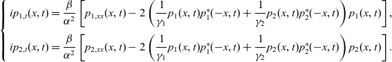 \begin{equation}\left \{\begin{array} {l}ip_{1,t}(x,t)= \dfrac {\beta }{\alpha ^2} \left[ p_{1,xx}(x,t) - 2\left(\dfrac 1 {\gamma_1 } p_1(x,t) p_1^* (-x,t) + \dfrac 1 {\gamma_2 } p_2(x,t) p_2^* (-x,t)\right) p_1(x,t) \right],\\ \\[-7pt] ip_{2,t}(x,t)= \dfrac {\beta }{\alpha ^2} \left[ p_{2,xx}(x,t) - 2\left(\dfrac 1 {\gamma_1 } p_1(x,t) p_1^* (-x,t) + \dfrac 1 {\gamma_2 } p_2(x,t) p_2^* (-x,t)\right) p_2(x,t) \right].\end{array} \right.\end{equation}
According to our formulation of solutions above, this system has the following one-soliton solution:
 \begin{equation}\left \{\begin{array} {l}\displaystyle p_1(x,t)=\dfrac { \alpha (\lambda _1 +\lambda _1^*) w_{1,1}w_{1,2}^* }{ |w_{1,1}|^2 \textrm{e}^{ i [ \alpha \lambda _1 ^* x - \beta(\lambda _1^*) ^2 t ] }+ (\gamma _1 |w_{1,2}|^2 +\gamma _2 |w_{1,3}|^2 ) \textrm{e}^{ - i(\alpha \lambda _1 x +\beta \lambda _1 ^2 t ) } },\\ \\ \displaystyle p_2(x,t)=\dfrac { \alpha (\lambda _1 +\lambda _1^*) w_{1,1}w_{1,3}^* }{ |w_{1,1}|^2 \textrm{e}^{ i [\alpha \lambda _1 ^* x -\beta (\lambda _1^*) ^2 t ] }+ (\gamma _1 |w_{1,2}|^2 +\gamma _2 |w_{1,3}|^2 ) \textrm{e}^{ - i( \alpha \lambda _1 x + \beta \lambda _1 ^2 t ) } },\end{array} \right.\end{equation}
provided that
 $w_{1}=(w_{1,1},w_{1,2},w_{1,3})^T$
satisfies the orthogonal conditions:
$w_{1}=(w_{1,1},w_{1,2},w_{1,3})^T$
satisfies the orthogonal conditions:
 \begin{equation*}w_{1,1}^2 +\gamma_1 w_{1,2}^2+\gamma_2 w_{1,3}^2=0,\ |w_{1,1}|^2+\gamma_1 |w_{1,2}|^2+\gamma_2 |w_{1,3}|^2=0.\end{equation*}
Note that the product
 $\gamma_1 \gamma_2$
could be either positive or negative.
$\gamma_1 \gamma_2$
could be either positive or negative.
5 Concluding remarks
The paper aims to present a class of non-local reverse-space integrable matrix non-linear Schrödinger (NLS) equations and their inverse scattering transforms. The main analysis is based on Riemann–Hilbert problems associated with a kind of arbitrary-order matrix spectral problems with matrix potentials. Through the the Sokhotski–Plemelj formula, the associated Riemann–Hilbert problems were transformed into Gelfand–Levitan–Marchenko-type integral equations, and the corresponding reflectionless problems were solved to generate soliton solutions for the non-local reverse-space matrix NLS equations.
The Riemann–Hilbert technique, which is very effective in generating soliton solutions (see also, e.g., [Reference Liu and Guo22, Reference Yang48]), has been recently generalised to solve various initial-boundary value problems of continuous integrable equations on the half-line and the finite interval [Reference Fokas and Lenells11, Reference Lenells and Fokas23]. There are many other approaches to soliton solutions that work well and are easy to use, among which are the Hirota direct method [Reference Hirota19], the generalised bilinear technique [Reference Ma25], the Wronskian technique [Reference Freeman and Nimmo17, Reference Ma and You33] and the Darboux transformation [Reference Ma and Zhang35, Reference Matveev and Salle40]. It would be significantly important to search for clear connections between different approaches to explore dynamical characteristics of soliton phenomena.
We also emphasise that it would be particularly interesting to construct various kinds of solutions other than solitons to integrable equations, such as positon and complexiton solutions [Reference Ma24, Reference Matveev41], lump and rogue wave solutions [Reference Ma and Zhou38]–[Reference Ma31], Rossby wave solutions [Reference Zhang and Yang50], solitonless solutions [Reference Ma28, Reference Ma29, Reference Rybalko and Shepelsky43] and algebro-geometric solutions [Reference Belokolos, Bobenko, Enol’skii, Its and Matveev7, Reference Ma26], from a perspective of the Riemann–Hilbert technique. Another interesting topic for further study is to establish a general formulation of Riemann–Hilbert problems for solving generalised integrable equations, for example, integrable couplings, super integrable equations and fractional analogous equations.
Acknowledgements
The work was supported in part by NSFC under the grants 11975145 and 11972291, the Fundamental Research Funds of the Central Universities (grant no. 2020MS043), and the Natural Science Foundation for Colleges and Universities in Jiangsu Province (grant no. 17 KJB 110020). The authors are also grateful to the reviewers for their constructive comments and suggestions, which helped improve the quality of their manuscript.
Conflict of interest
None.
