Terrestrial snow cover occupies higher latitude areas of the Northern Hemisphere (NH) from several up to 9 months each year in the Arctic land surface, with significant influence on the surface energy budget, subsoil thermal regime, and the freshwater storage. Snow cover also interacts with vegetation and affects terrestrial habitats and species.
2.1 History
The hexagonal form of snowflakes was first noted by Johannes Kepler in 1611. Robert Hooke revealed the variety of crystalline structures as seen through a microscope in 1665. Similar studies were performed in the mid-eighteenth century in France and England. Reference Bentley and HumphriesBentley and Humphries (1931) published a book with over 2,500 illustrations of snowflake photographs of variety of snow crystals.
The earliest snow surveys were made at Mt. Rose, Nevada, in 1906 by James Church, and by 1909–1910 a network of stations was being surveyed by him. Snow surveys provide an inventory of the total amount of snow covering a drainage basin or a given region. Church also invented the Mt. Rose sampler – a hollow steel tube designed so that each inch of water in the sample weighs 1 ounce (28.35 g). Snow surveying began at locations in several western states between 1919 and 1929 and in the latter year California organized cooperative snow surveys (Reference StaffordStafford, 1959).
In 1931, a permanent Committee on the Hydrology of Snow was organized in the Hydrology section of the American Geophysical Union, chaired until 1944 by Dr. Church. By 1951, there were about one thousand snow courses in the western states and British Columbia. A snow course comprises an area demarcated for measuring the snow periodically during each snow season. Usually three to eight samples are taken and averaged to determine the snow depth and snow water equivalent (SWE) for that location. Stream flow forecasting to assess water supply is the primary objective. In remote locations, aerial markers were installed; these are vertical markers with equally spaced crossbars. The depth of snow is determined by visual observation from low-flying aircraft. The number of snow courses has declined considerably in recent years in part due to the extension of the Snow Telemetry (SNOTEL) network. These are automated weather stations designed to operate in severe, remote mountainous environments. Most sites collect daily, or even hourly, SWE and precipitation, and relay it by meteor burst technology to collection stations in Boise, Idaho, or Portland, Oregon.
Remote sensing of snow cover by the Very High Resolution Radiometer (VHRR) of National Oceanic and Atmospheric Administration (NOAA) that began in 1966 and its continuation – the Advanced VHRR (AVHRR) – provides the longest time series of hemispheric snow cover data. Spaceborne passive microwave measurements were applied to estimate snow depth and SWE in the late 1970s, as discussed later in this chapter. The Cold Land Processes Experiment (CLPX) of NASA took place in the winter of 2002 and spring of 2003, in the central Rocky Mountains of the western United States where there is a rich array of different terrain, snow, soil, and ecological characteristics to test and improve algorithms for mapping snow. Through the field campaigns of CLPX, algorithms for SWE retrieval and soil freeze–thaw status from spaceborne passive microwave sensors, and radar retrieval algorithms for snow depth, density, and wetness were evaluated and improved. The data were also used to improve spatially distributed, uncoupled snow/soil models and coupled cold land surface schemes.
The National Operational Hydrologic Remote Sensing Center (NOHRSC) of NOAA in the United States developed the airborne mapping of SWE using surface-emitted gamma radiation from potassium, uranium, and thorium radioisotopes in the soil. Gamma radiation is attenuated by snow cover and absorbed by water in the snowpack (NWS, 1992), and so to estimate SWE, both gamma counts and soil moisture over snow and bare ground are needed. Such SWE data had been used to develop passive microwave retrieval algorithms (e.g., Reference Singh and GanSingh and Gan, 2000). Snow depth can also be estimated by microwave radiation transfer models, such as that of Reference Chang, Foster and HallChang et al. (1987), even though such models may underestimate the snow depth, as Reference ButtButt (2009) found in a study in the United Kingdom.
2.2 Snow formation
Snow
The creation of saturation conditions necessary for the formation of water droplets or ice particles occur mainly through convection or updraft, cyclonic cooling induced by circulation, frontal or non-frontal lifting of warm air, or orographic cooling by mountain barriers. Snow forms primarily through heterogeneous nucleation. This process involves air that is saturated with a temperature below 0 °C. Water vapor condenses and solidifies, or vapor is deposited on nuclei, which grow into ice and snow crystals. These freezing nuclei may be clay mineral dust (kaolinite, e.g., becomes active at −9 °C), aerosols, pollutants, ice crystal splinters from clouds above, or artificial seeding agents (solid CO2 or “dry ice,” silver iodide, or urea). The crystals may continue growing through interactions between crystals (crystal aggregation) or with supercooled water droplets, a process called riming (the capture of supercooled cloud droplets by snow crystals) to form snow pellets and/or snowflakes (Reference MosimannMosimann et al., 1993). The minimum size of ice crystals involved in riming is ~60 μm diameter for hexagonal plates and 30 μm width and 60 μm length for columnar ice crystals (Reference ÁvilaÁvila et al., 2009). Under extremely low temperatures (below −40 °C), ice particles can also be formed by the spontaneous freezing of water molecules, which is called “homogeneous nucleation.” Homogeneous nucleation of water droplets occurs at −40 °C; at −10 °C approximately 1/106 drops freeze and at −30 °C about 1/103 drops freeze.
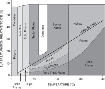
Ice crystal shapes are hexagonal in form from 0 °C to −80 °C and cubic form from −80 °C to −130 °C. The reason is that an oxygen molecule is tetrahedral; two together form a hexagon or tetrahedra offset by 60° form a cubic crystal. A cubic crystal will transform to a hexagon if warmed but not vice versa. Crystal types have a dependence on temperature and saturation vapor pressure over ice. Under various combinations of temperature and supersaturation conditions with respect to ice, a wide range of snowflakes/pellets results (Figure 2.1). In general, as the temperature decreases, plates → needles → prisms. They can be broadly classified as dendritic and sector plates that involve crystal growth on the a-axis (horizontal), or columns (prisms and needles) that involve growth on the c-axis (vertical) (Figure 2.1). Reference MasonMason (1994) suggests that transitions between crystal types in clouds can lead to more effective release of precipitation through the formation of precipitation elements that have a better chance of surviving below-cloud-base evaporation.

Figure 2.1 Types of snow crystals resulting from various combination of temperature and supersaturation.
Snowfall
Whenever snow crystals grow to a size when gravitational pull exceeds the buoyancy effect of air, snowfall occurs. Snowfall typically reaches the ground when the freezing level is not higher than about 250 m above the surface, and the surface air temperature averages ≤1.2 °C. Snow may fall as snowflakes, snow grains (the solid equivalent of drizzle; white, opaque ice particles ≤1 mm in diameter), or graupel (snow pellets of opaque conical or rounded ice particles 2–5 mm in diameter formed by aggregation).
Snowflakes
Snowflakes can be classified into many types (Reference Grey, Prowse and MaidmentGrey and Prowse, 1993; Reference Sturm, Holmgren and ListonSturm et al., 1995). Snowflakes form through the growth of ice crystals by the accretion of water vapor and by their aggregation in branched clusters. The saturation vapor pressure is lower over an ice surface than a water surface, reaching a maximum difference of 0.12 mb at −12 °C. As a result, in a mixed phase cloud, supercooled water droplets tend to evaporate and vapor is deposited onto ice crystals. This is known as the Bergeron–Findeisen process after its discoverers. Snowflakes grow in small cap clouds over elevated terrain when ice crystals falling from an upper cloud layer seed them. This is known as the seeder–feeder mechanism (Reference BarryBarry, 2008, p. 273). Ice crystals may float in the atmosphere as “diamond dust” when the air temperature is ≤−40 °C. The design and variations of snowflakes are way beyond human imaginations, as some examples in Figure 2.2 that show needle, sheath, and varieties of stellar crystals with plates, dendritic, and sector-like branches. Bentley, who was born in 1865, even believed that no two snowflakes are exactly alike (Reference TeelTeel, 1994).
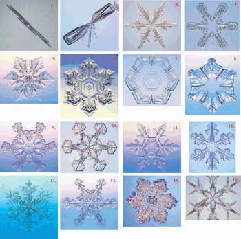
Figure 2.2 Examples of snowflakes classified according to Reference Magono and LeeMagono and Lee (1966): 1. Needle, 2. Sheath, 3. Stellar crystal, 4. Stellar crystal with sector-like ends, 5. Stellar crystal with plates at ends, 6. Crystal with broad branches, 7. Plate, 8. Plate with simple extension, 9. Plate with sector-like ends, 10. Rimed plate with sector-like ends, 11. Hexagonal plate with dendritic extensions, 12. Plate with dendritic extensions, 13. Dendritic crystal, 14. Dendritic crystal with sector-like ends, 15. Rimed stellar crystal with plates at ends, and 16. Stellar crystal with dendrites
Depth hoar
Other than in permafrost areas (high latitudes or high elevations in middle latitudes), the ground is mostly warm or near freezing when the ground is snow covered. This is true even when the air is very cold, because snow is a good insulator. Therefore, there will usually be liquid water in the snowpack, and it is common for the snow near the ground to remain damp for most of the winter. Depth hoar forms at the base of a snowpack, as a result of large temperature gradients between the warm ground and the cold snow surface, when rising water vapor freezes onto existing snow crystals. It usually requires a thin snowpack combined with a clear sky or low air temperature, and it grows best at snow temperatures from −2 °C to −15 °C. Therefore, the occurrence of depth hoar is common in high Arctic regions such as Alaska, the Northwest Territory, Nunavut, and northern Siberia (Reference DerksenDerksen et al., 2009). Depth hoar constitutes about 20% of all snow layers in the high Arctic (46% in sub-Arctic), an average grain size of 6.5 mm (long-axis) and 2 mm (short-axis), and about 0.23 gm cm−3 in density (Reference DerksenDerksen et al., 2014).
Depth hoar consists of sparkly, large-grained, faceted, cup-shaped ice crystals up to 10 mm in diameter. Beginning and intermediate facets are 1–3 mm square; advanced facets can be cup-shaped 4–10 mm in size. Larger-grained depth hoar is more persistent and can last for weeks. Depth hoar is strong in compression but not so in shear, and hence often behaves like a stack of champagne glasses; it can fail in the form of collapsing layers, or in shear, with fractures often propagating long distances and around corners. Even though the stability of the snowpack depends on the cohesion between layers of snow and meteorological factors, almost all catastrophic avalanches, which involve the entire season’s snow cover, fail on depth hoar layers (Reference TremperTremper, 2008). Seismic sensors have been used for the remote detection of snow avalanches for they can also estimate avalanche velocity, size, and type (Reference LacroixLacroix et al., 2012).
2.3 Snow cover
Introduction
Snow is an integral component of the global climate system because of its linkages and its feedback between surface energy, moisture fluxes, clouds, precipitation, hydrology, and atmospheric circulation (Reference King, Armstrong and BrunKing et al., 2008). It is the most spatially extensive and seasonally variable component of the global cryosphere (see Table 1.1). On an average, snow covers almost 50% of the Northern Hemisphere’s land surface in late January, with an August minimum of about 1%. In addition, there is perennial snow cover over the Antarctic ice sheet (12 million km2) and at the higher elevations of the Greenland Ice Sheet (about 0.6 million km2) (Figure 2.3).
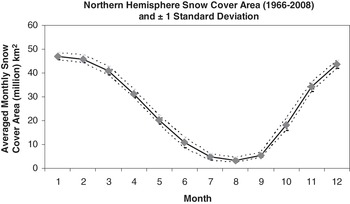
Figure 2.3 Averaged monthly snow cover area of Northern Hemisphere in (×106) km2 calculated from weekly snow cover extent maps produced primarily from daily visible satellite imagery of NOAA-AVHRR by the Rutgers Global Snow Lab
Since snow produces substantial changes in the surface characteristics, and the atmosphere is sensitive to physical changes of the earth surface, its presence over large areas of the Earth for at least part of the year exerts an important influence on the climate, both locally and globally. The best-known effect involves the albedo–temperature positive feedback, whereby an expanded (reduced) snow cover increases (decreases) the reflection of incoming solar radiation, reducing (increasing) the temperature, and thereby encouraging an expansion (reduction) of the snow cover. Fresh snow has a spectrally integrated albedo of 0.8–0.9, making it the most reflective natural surface. This value decreases with age to 0.4–0.7 as the snow density increases through settling and snow metamorphism and is reduced still further by impurities in or on the snow (e.g., mineral dust, soot, aerosols, biogenic matter) (see Figure 2.4). The cooling effect of snow cover is illustrated by the example that, in the Upper Midwest of the United States, winter months with snow cover are about 5–7 °C colder than the same months without snow cover. Snow, a poor conductor of heat, also insulates the soil surface and sea ice. Therefore, a better knowledge of the snow cover and its properties over large regions will lead to a better understanding of our climate.
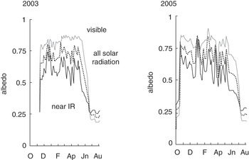
Figure 2.4 Field measurements of broadband albedo at Mammoth Mountain in the Sierra Nevada for (a) 2003 and (b) 2005, showing albedo in the visible, near-infrared and all solar radiation
Snow is held in cold storage until there is sufficient energy to melt it to water or to sublimate it to water vapor. The storage of water in the seasonal snow cover introduces into the hydrological cycle an important delay of weeks to months, causing a peak in the annual runoff in spring and early summer when the river water is agriculturally more valuable. It is highly beneficial to be able to estimate the amount and timing of release of this stored precipitation to spring runoff, which allows a better management of water resources for irrigation and hydroelectric production planning. The dynamics of water storage in seasonal snowpack is also critical to the effective management of water resources globally. Snow water accumulated in winter in the Arctic river basins is critical for the springtime snowmelt, and the freshwater from its river systems accounts for about 50% of the net flux of freshwater into the Arctic Ocean (Reference Barry, Serreze and LewisBarry and Serreze, 2000), which is a large percentage when compared to the freshwater inputs to the tropical oceans, where freshwater input is dominated by direct precipitation. Frozen soil affects the snowmelt runoff and soil hydrology by reducing the soil permeability. Runoff affects ocean salinity and sea ice conditions (Reference PetersonPeterson et al., 2002), and the degree of surface freshening can affect the global thermohaline circulation (Reference BroeckerBroecker, 1997). In future, we expect even larger freshwater input from the Arctic as the global hydrologic cycle accelerates, higher precipitation is expected in high latitudes and higher runoff from Arctic river basins (Reference Nummelin, Ilicak, Li and SmedsrudNummerlin et al., 2016).
Snowpacks affect energy and water exchanges, and so both snow cover and SWE are important climatic and hydrologic variables. In particular, snow controls the climate and hydrology of the cryosphere and higher latitude regions significantly, and the amount and distribution of snow is affected by the climate and vegetation types. In the Canadian Prairies, mixed precipitation can occur within a certain range of temperature (Reference KienzleKienzle, 2008), but on a whole approximately one-third of its annual precipitation occurs as snowfall, and the shallow snow cover generates as much as 80% of the annual surface runoff. In the Colorado Rockies, the Sierra Nevada of California, and the Cascade Mountains of Washington, snowmelt can account for up to 65–80% of the annual water supply (Reference SerrezeSerreze et al., 1999), but shifts in snowmelt runoff due to climate warming is expected to affect water supply in snow-dominated river basins (Reference FosterFritz et al., 2011).
The snow covers of North America (NA) and Eurasia change seasonally, in accordance with the position of the Sun that shines directly at the Tropic of Cancer in the Northern Hemisphere (NH) on June 21 (summer solstice) and then moves southward, reaching the Tropic of Capricorn in the Southern Hemisphere on December 22 (winter solstice), before moving northward for the next 6 months; the cycle repeats itself on an annual time scale. The extent of snow cover in the NH lands reaches an average maximum of about 46.8 × 10⁶ km2 in January and February, and an average minimum of about 3.4 × 10⁶ km2 in August (see Figure 2.5) (Reference RopelewskiRopelweski, 1989; Reference Brown, Armstrong, Armstrong and BrunBrown and Armstrong, 2008; Reference RobinsonRobinson, 2008), which constitute 8% and about 0.5% of the Earth’s surface, respectively. From 1966 to 2008, the maximum January snow cover of NH ranged from as low as 42 × 106 km2 (in 1982) to as high as 50.1 × 10⁶ km2 (in 2008) (GSL, 2008). For 1966–2008, the mean annual NH snow extent was 25.5 × 10⁶ km2 (Reference RobinsonRobinson, 2008). The 1967–2016 mean annual NH snow extent was lower after mid-1980s relative to what it was before the mid-1980s. Even though the linear trend estimated was − 25,000 km2 per year, this is due to a step-like drop in the mid-1980s, for the decline of NH snow cover is nonlinear, and above-average snow cover was even observed in 2015–2016 (Reference ConnollyConnolly et al., 2019).
Figure 2.5 Seasonal variation in the mean monthly snow and sea ice cover extent for January, April, and July over Northern Hemisphere using data of NSIDC over 1967–2005 for snow and 1979–2005 for ice; for January and July over Antarctic/Southern Hemisphere over 1987–2002 for snow and 1979–2003 for ice (Reference MaurerMaurer, 2007) by Lambert Azimuthal Equal-Area (http://nsidc.org/data/atlas) projection; January 31, 2008 snow and ice chart of NH
In the NH, most mid-summer snow cover is found over the Greenland and some parts of the Canadian High Arctic (Figure 2.5a), while about 60% of winter snow cover is found over Eurasia and 40% over Canada and the upper portion of the United States, sometimes down to latitude 30° N (Figure 2.5c). Figure 2.6 is a composite monthly NOAA-AVHRR image of NA that shows large seasonal variations in snow cover between the four seasons. In contrast, in South America, there is only a small area covered with snow in July.
Figure 2.6 Seasonal variation in the mean monthly snow cover extent for (a) July, (b) October, (c) January, and (d) April over North America computed from snow charts derived from weekly visible satellite images of NOAA-AVHRR over 1972–1993 (www.tor.ec.gc.ca/CRYSYS/cry-edu.htm); (e) Northern Hemisphere snow and forest covers for January, 2005 computed from the NSIDC Equal-Area Scalable Earth Grid (EASE-Grid) snow cover product (Armstrong and Brodzik, 2005) and the University of Maryland global land cover classification
Snow cover is observed in situ at hydrometeorological stations, from daily depth measurements, (monthly) snow courses, and in special automated networks such as about 730 SNOwpack TELemetry (SNOTEL) automated systems of snow pressure pillows, sonic snow depth sensors, precipitation gauges, and temperature sensors distributed across the United States. The extent of snow cover is also observed and mapped daily (since June 1999) over the NH from the operational satellites of the NOAA, United States.
Canada has extensive in situ snow depth and snow course networks that are a valuable database for monitoring cryospheric changes and for validating satellite data such as those shown in Figures 2.5 and 2.6. However, most of the field observations are concentrated in southern latitudes and lower elevations, where the majority of the population lives. At many northern sites, manned stations have been replaced by automatic weather station (AWS) that use acoustic sounders to measure the height of the snow surface.
Besides seasonal variability, snow cover is subject to inter-annual fluctuations but only about 40% of these have been found to be associated with continental to hemispheric scale forcing (Reference Robinson, Frei and SerrezeRobinson et al., 1995), and the rest could be partly attributed to regional forcings or “coherent” regions. Regarding the boreal winter variability, Reference Saito and CohenSaito and Cohen (2003) noted that snow cover at continental scale varies similarly as the inter-annual to inter-decadal oscillations of an internal mode of the atmosphere, but it leads the atmosphere by several months through their mutual oscillations. By principal component analysis (PCA) and composite analysis, Reference Frei and RobinsonFrei and Robinson (1999) found that over western NA, snow cover extent (SCE) is associated with the longitudinal North American ridge, the Pacific North America (PNA) index, while over eastern NA, it is associated with the meridional oscillation of the 500-mb geopotential height, the North Atlantic Oscillation (NAO), and the teleconnection patterns are coupled to tropospheric variability during autumn and winter. Reference Gobena and GanGobena and Gan (2006) found during El Niño winters, the southeasterly flow of warm dry Pacific air and the northwesterly flow of cool dry Arctic air will be the dominant flow over western Canada and Pacific Northwest (PNW) of the United States, giving rise to drier climate (less snowfall) over these regions. On the other hand, La Niña winters are associated with an erosion of the western Canadian ridge and strengthening of the Pacific Westerly, giving rise to greater moisture supply and so more winter snowpack in western Canada and the PNW of the United States. For Europe, Reference Henderson and LeathersHenderson and Leathers (2010) found that large (small) snow extent is associated with negative (positive) 850 hPa zonal wind anomalies, negative (positive) phase of the North Atlantic Oscillation, negative (positive) 1,000–500 hPa thickness anomalies, and generally positive (negative) Northern European precipitation anomalies. Besides solar radiation, snowpacks are related to surface air temperature, precipitation, storm tracks, and mid-tropospheric geopotential heights at 500 mb. Reference Frei and RobinsonFrei and Robinson (1999) postulate that snow extent, by exerting an influence on lower tropospheric dynamics (e.g., air temperature), could even modulate atmospheric circulations.
Reference BrownBrown (2000) observed some decline in NH snow cover in recent decades, but the declines are not statistically significant. From 1972 to 2000, using weekly NH snow cover data of high latitude and high elevation areas derived from visible bands of NOAA satellite observations, Reference DyeDye (2002) found that the week of the last-observed snow cover in spring shifted earlier by 3–5 days per decade estimated from a linear regression analysis, and the duration of the snow-free period increased by 5–6 days per decade, primarily as a result of earlier snow cover disappearance in spring. Similarly, based on the 1966–2007 snow cover data of NOAA satellites and simulations from the Coupled Model Intercomparison Project Phase 3 Model (CMIP3), on the response of NH land area with seasonal snow cover to warming and increasing precipitation, Reference Brown and MoteBrown and Mote (2009) found the largest decrease in snow cover duration (SCD) was concentrated in zones where seasonal mean air temperatures were in the range of −5 to +5 °C, which extended around the mid-latitudinal coastal margins of the continents. Regional studies in the western United States (e.g., Reference Adam, Hamlet and LettenmaierAdam et al., 2009) show that losses of snowpack associated with warming trends have been ongoing since the mid-twentieth century, especially near boundaries of areas that currently experience substantial snowfall. These findings very likely reflect clear signals of human-induced impact on the climate shown by the changing snowpacks of NH and by the river flows of western United States (Reference Barnett, Pierce, Hidalgo, Bonfils, Santer, Das, Bala, Wood, Nozawa, Mirin, Cayan and DettingerBarnett et al., 2008), and Reference Brown and RobinsonBrown and Robinson (2011) detected significant contractions of snow cover in NH over 1922–2010.
According to the CMIP5 Report, observed SCE has decreased in the NH, especially in spring (Reference Vaughan and StockerVaughan et al., 2013). Satellite records indicate that over the period 1967–2012, the annual mean SCE negative trend is statistically significant, with the largest change of −53% (−40% to −66%) occurred in June. Over 1922–2012, the available snow cover data for March and April show a 7% decline and a strong negative (−0.76) correlation with the March–April 40° N to 60° N land temperature. The spring SCE in Arctic land areas north of 60° N has significantly declined since 1960s, estimated respectively at −3.5% in May and −13.4% in June per decade between 1981 and 2018, relative to the 1981–2010 mean, from multiple data sets (SROCC, 2019). From surface observations, satellite data, and model-based analyses, the snow cover duration has also become shorter, between −0.7 and −3.9 days per decade depending on region and time period, but all spring snow cover duration trends from all data sets are negative (Reference Bulygina, Groisman, Razuvaev and KorshunovaBulygina et al., 2011; Reference Liston and HiemstraListon and Hiemstra, 2011; Reference Estilow, Young and RobinsonEstilow et al., 2015). These same multisource data sets also identify reductions in autumn snow extent and duration at −0.6 to −1.4 days per decade (Reference Brown, Vikhamar-Schuler, Bulygina, Derksen, Loujus and MudrykBrown et al., 2017). The CMIP6 report will provide further updates on observed snow cover changes (Reference Eyring, Bony, Meehl, Senior, Stevens, Stouffer and TaylorEyring et al., 2016).
The mountain snow cover is characterized by a very strong interannual and decadal variability (Reference Mankin and DiffenbaughMankin and Diffenbaugh, 2015). Long-term in situ snow cover data are limited in some regions, particularly in High Mountains of Asia and Northern Asia. For key mountainous regions, Reference StewartStewart (2009) found that higher temperatures have decreased snowpack and resulted in earlier melt in spite of precipitation increases at mid-elevation regions but not at high-elevation regions, which remain well below freezing during winter. Mountain snow cover at lower elevations has generally declined in duration by about several days per decade mainly due to more precipitation falling as rain and to higher melt rate at most elevations, mostly due to increased air temperature (Reference Marty, Tilg and JonasMarty et al., 2017). The mean snow depth and SWE have declined since the mid-twentieth century, with regional variations but at higher elevation, snow cover trends are generally insignificant (SROCC of Reference Pörtner, Roberts, Masson-Delmotte, Zhai, Tignor, Poloczanska, Mintenbeck, Nicolai, Okem, Petzold, Rama and WeyerIPCC, 2019).
At lower elevations in the European Alps, Western North America, Himalaya, and subtropical Andes, the snow depth or mass is projected to decline by 25% between the recent past period (1986–2005) and the near future (2031–2050). By 2081–2100, reductions of up to 80% are expected under RCP8.5, 50% under RCP4.5, and 30% under RCP2.6 climate scenarios of CMIP5 (SROCC of Reference Pörtner, Roberts, Masson-Delmotte, Zhai, Tignor, Poloczanska, Mintenbeck, Nicolai, Okem, Petzold, Rama and WeyerIPCC, 2019, ch. 2). At higher elevations, projected reductions are smaller as temperature increases at higher elevations mainly affect the ablation component of snow mass evolution. The projected increase in wintertime snow accumulation may even result in a net increase in winter snow mass. All elevation levels and mountain regions are projected to exhibit sustained interannual variability of snow conditions throughout the twenty-first century.
Snow cover, depth distribution, and blowing snow
At continental scale or larger, snow cover distribution primarily depends on latitude and seasons (Figures 2.5 and 2.6). At the macro or regional scale, for areas up to 106 km2, and distances from 10 to 1,000 km, snow cover distribution depends on latitude, elevation, orography, and meteorological factors. For example, snowfall caused by orographic cooling tends to increase with a rise in elevation, and frontal activities involving cold fronts generally produce more intense snowfall over relatively smaller areas as against warm fronts that produce moderate or light snowfall over larger areas, because the former has relatively steep leading edge while the latter has mild leading edge. On the mesoscale, with distances of 100 m to 10 km, snow distribution depends on the blowing effect of wind, relief, and vegetation patterns, while on the microscale, 10–100 m, the influencing factors are more local. Over highly exposed terrain, the effects of meso- and microscale differences in vegetation and terrain features may produce wide variations in accumulation patterns and snow depths.
Blowing snow occurs when the force of wind exceeds the shear strength of the snowpack surface that resists snow particles to move. Blowing snow increases with wind speeds and the amount of snowfall but decreases with increasing surface roughness. The effects of wind on the accumulation and distribution of a snowpack are most pronounced in open environments, for example, the Canadian Prairies or Siberian steppes, with three modes of snow particle movement: snow particles begin in motion by creeping or rolling on snowpack surface, then by saltation or bouncing when wind speed increases, and finally in turbulent diffusion or snow particles suspended in the air under high wind speed. These three modes of transport typically occur less than 1 cm above ground under a low wind speed U < 5 m s−1, between 1 and 10 cm for U = 5–10 m s−1, and between 1 and 100 m for U > 10 m s−1, respectively.
Based on wind tunnel studies with surface wind speeds of up to 40 m s−1, Reference DyuninDyunin et al. (1977) argued that saltation accounts for most drifting snow at all conceivable wind speeds. However, Reference Budd, Dingle and RadokBudd et al. (1964) found that turbulent suspension was the primary mechanism from snowdrift studies at Byrd Station, Antarctica. Suspension increases at about U4, whereas saltation increases linearly with U at high wind speeds (at which most transport occurs), so suspension dominates the overall effect of wind (Reference Pomeroy and GrayPomeroy and Gray, 1990; Pomeroy, p.c. December 2009). At low wind speeds, saltation is the dominant process.
Blowing snow is important in open environments, especially for high elevation alpine areas above treeline, in the Prairies, and in the tundra of the North American Arctic and Siberia. In these regions snow depth variation depends mainly on terrain features because without the hindering effect of vegetation cover, wind causes snow drift and redistribution to smooth topography, so that mountain tops and plateau tend to have thin snowpack as snow tends to be blown to valleys and low-lying areas which as a result tend to have relatively thick snowpack. In the coastal tundra and open subarctic forest near Churchill, Manitoba of Canada, Reference Kershaw and McCullochKershaw and McCulloch (2007) found that snowpack characteristics measured from 2002 to 2004 also depend on vegetation characteristics, ecosystems, and associated micro-climates. Ecosystems that dominate the circumpolar north are such as wetland, black and white spruce forest, burned forest, forest-tundra transition, and tundra. In lower latitudes as the forest canopy density generally increases, higher snow accumulation has been found in forests of medium density (25–40%) than large open areas because of reduced wind effects by densely forested areas (e.g., Reference VeatchVeacth et al., 2009). Although forest structure and canopy interception, and local terrain characteristics will influence snow retention at local scales, Reference LundquistLundquist et al. (2013) show that where the mean DJF temperatures exceed −1 °C, forests with lower total canopy cover are likely to enhance snow retention by minimizing mid-winter and early spring melt.
Reference Gordon, Savelyev and TaylorGordon et al. (2009) developed a camera system to measure the relative blowing snow density profile near the snow surface in Churchill, Manitoba, and Franklin Bay, Northwest Territory. Within the saltation layer, they found that the observed vertical profile of mass density is proportional to exp(−0.61z/H), where H, the average height of the saltating particles, varies from 1.0 to 10.4 mm, while z, the extent of the saltation layer, varies from 17 to over 85 mm. At greater heights, z > 0.2 m, the blowing snow density varies according to a power law (ρs∝z−ɤ), with a negative exponent 0.5 < γ < 3. Between these saltation and suspension regions, results suggest that the blowing snow density decreases following a power law with an exponent possibly as high as γ≈8.
2.4 Snow cover modeling in land surface schemes of GCMs
Snow cover is treated in land surface models (LSMs), but snow and ice albedo parameterizations differ widely in their complexity (Reference BarryBarry, 1996), and more physically based schemes should generally result in better snow and ice albedo parameterization, which ideally should be validated against field measurements (Reference PirazzinniPirazzini, 2009). The Snow Model Intercomparison Project (SnowMIP) was conducted using 24 snow cover models developed in ten different countries (Reference Essery and YangEssery and Yang, 2001). The models differ from single versus multi-layers, with and without a soil model, variable versus constant heat conductivity and snow density, and the treatment of liquid storage. Only 4 of the 24 models met all the five criteria. However, more recent models have been developed to incorporate snow dynamics affected by soil–snow–vegetation interactions in forests (Reference EsseryEssery, 2013).
Twenty seven atmospheric general circulation models (GCMs) were run under the auspices of the Atmospheric Model Intercomparison Project (AMIP)-I. The GCMs of AMIP-I reproduced a seasonal cycle of snow extent similar to the observed cycle, but they tend to underestimate the autumn and winter snow extent (especially over North America) and overestimated spring snow extent (especially over Eurasia). The majority of models display less than half of the observed interannual variability. No temporal correlation is found between simulated and observed snow extent, even when only months with extremely high or low values are considered (Reference Frei and RobinsonFrei and Robinson, 1995). The second-generation AMIP-II simulations gave better results (Reference Frei, Miller and RobinsonFrei et al., 2003).
Reference SlaterSlater et al. (2001) found that various snow models in land surface schemes could model the broad features of snow cover and snowmelt processes for open grasslands on both intra- and interannual basis. On the other hand, modeling the spatial variability of snow cover is more problematic because this requires careful consideration of blowing snow transport and sublimation, canopy interception, and patchy snow conditions which are difficult to parameterize accurately. Reference Woo, Marsh and PomeroyWoo et al. (2000) made some progress in understanding some such processes at a local scale, but it is still a long way to incorporating field observations into land surface schemes and climate models where such processes have to be extended to spatial scales of the order of 10–100 km. Until now, most land surface schemes and climate models do not account for the subgrid variability of snow cover in each grid cell. There are new snow models developed in land surface schemes such as that of the European Centre for Medium-Range Weather Forecasts (ECMWF) that includes a new parameterization of snow density, incorporating a liquid water reservoir, and revised formulations for the subgrid snow cover fraction and snow albedo. The new scheme reduces the end of season ablation biases from 10 to 2 days in open areas and from 21 to 13 days in forest areas, and the albedo bias, and so reducing the average surface net shortwave radiation bias by 5.2 W m−2 in 14% of the NH land (Reference Dowdeswell, Hagen, Bamber and PayneDutra et al., 2010).
To realistically simulate grid-averaged surface fluxes, Reference ListonListon (2004) developed a Subgrid SNOW Distribution (SSNOWD) submodel that explicitly considers the changes of snow-free and snow cover areas (SCAs) in each surface grid cell as the snow melts, by assuming SWE distributes according to a lognormal distribution and the snow-depth coefficient of variation (CV). Using a dichotomous key based on air temperature, topographic variability, and wind speed, Liston proposed a nine-category, global distribution of subgrid snow-depth-variability, each category being assigned a CV value based on published data. The SSNOWD then separately computed surface-energy fluxes over the snow-covered and snow-free portions of each model grid cell, weighing the resulting fluxes according to these fractional areas. Using a climate version of the Regional Atmospheric Modeling System (ClimRAMS) over a North American domain, SSNOWD was compared with a snow-cover formulation that ignores sub-grid snow-distribution. The results indicated that accounting for snow-distribution variability has a significant impact on snow-cover evolution and associated energy and moisture fluxes.
Reference NittaNitta et al. (2014) incorporated SSNOWD into the Minimal Advanced Treatments of Surface Interaction and Runoff (MATSIRO) land surface model. Two 29-year global offline simulations, with and without SSNOWD, were performed while forced with the Japanese 25-year Reanalysis (JRA-25) data set combined with an observed precipitation data set. The snow cover fraction was improved by including SSNOWD, particularly for the accumulation season and/or regions with relatively small amounts of snowfall. In the NH, the daily snow-covered area simulated largely agree with the Interactive Multisensor Snow and Ice Mapping System (IMS) snow analysis data sets, and the seasonal cycle in the NH was improved because SSNOWD formulates the snow cover fraction differently for the accumulation and ablation seasons, and represents the hysteresis of the snow cover fraction between different seasons.
Modeling blowing snow
Reference Pomeroy, Gray and LandinePomeroy et al. (1993) developed the first comprehensive blowing snow model for the prairies environment. It estimates saltation, suspension and sublimation using readily available meteorological data. They show that within the first 300 m of fetch, transport removes 38–85% of the annual snowfall. However, beyond 1 km of fetch, sublimation losses from blowing snow dominate over transport losses. In Saskatchewan, sublimation losses are 44–74% of annual snowfall over a 4-km fetch. Subsequently, Reference PomeroyPomeroy (2000) showed that the ratio of snow removed and sublimated by blowing snow to that transported at prairies (arctic) sites was 2:1 (1:1), respectively.
Reference Essery, Long and PomeroyEssery et al. (1999) developed a distributed model of blowing snow transport and sublimation to consider physically based treatments of blowing snow and wind over complex terrain for an Arctic tundra basin. By considering sublimation, which typically removes 15–45% of the seasonal snow cover, the model is able to reproduce the distributions of snow mass, classified by vegetation type and landform, which they approximated with lognormal distributions. The representation used for the downwind development of blowing snow with changes in wind speed and surface characteristics is shown to have a moderating influence on snow redistribution. Spatial fields of snow depth have power spectra in one and two dimensions that occur in two frequency intervals separated by a scale break between 7 and 45 m (Reference Trujillo, Ramirez and ElderTrujillo et al., 2007). The break in scaling is controlled by the spatial distribution of vegetation height when wind redistribution is minimal and by the interaction of the wind with surface concavities and vegetation when wind redistribution is dominant.
Reference Liston and SturmListon and Sturm (1998) developed a SnowTran-3D that simulates wind-driven snow-depth evolution over topographically variable terrain and tested it in an arctic–tundra landscape, for it is generally applicable to treeless areas characterized by strong winds, below-freezing temperatures, and solid precipitation. Reference LawlerListon et al. (2007) extended the SnowTran-3D to version 2.0 that simulates wind-related snow distributions over the range of topographic and climatic environments globally. This version includes three primary enhancements to the original model: (1) an improved wind sub-model, (2) a two-layer sub-model describing the spatial and temporal evolution of friction velocity that must be exceeded to transport snow, and (3) a 3-D, equilibrium-drift profile sub-model that forces snow accumulations to duplicate observed drift profiles.
In mountainous regions, wind plays a prominent role in determining snow accumulation patterns and turbulent heat exchanges, strongly affecting the timing and magnitude of snowmelt runoff. Reference Winstral and MarksWinstral and Marks (2002) use digital terrain analysis to quantify aspects of the upwind topography related to wind shelter and exposure. They develop a distributed time-series of snow accumulation rates and wind speeds to force a distributed snow model. Terrain parameters were used to distribute rates of snow accumulation and wind speeds at an hourly time step for input to ISNOBAL, an energy and mass balance snow model that accurately modeled the observed snow distribution (including the formation of drifts and scoured wind-exposed ridges) and snowmelt runoff. In contrast, ISNOBAL forced with spatially constant accumulation rates and wind speeds taken from the sheltered meteorological site at Reynolds Mountain in southwest Idaho, a typical snow-monitoring site, overestimated peak snowmelt runoff, and underestimated snowmelt inputs prior to the peak runoff.
2.5 Snow interception by canopy
Snowfall can be intercepted by an over-story canopy and below the treeline, snow depth variation depend more on land use or vegetation types such as coniferous or broadleaf forests with different canopy structure (Reference GanGan, 1996). Snow falling into a canopy is influenced by two possible phenomena: (1) turbulent air flow above and within the canopy may lead to variable snow input rates and microscale variation in snow loading on the ground, (2) direct interception of snow by the canopy elements may either sublimate or fall to the ground. Interception processes are related to vegetation type (deciduous or evergreen), vegetation density, needle characteristics, canopy form and area, branch orientation, leaf area index (LAI), and the presence of nearby open areas. Increasing air temperature tends to increase the cohesiveness of snow and so increase the amount of intercepted snow retained in canopy. For forested environments, most studies show greater snow accumulation in open areas than in forest even though redistribution of intercepted snow by wind to clearings is not typically a significant factor. Instead, interception by canopy and subsequent sublimation, which constitutes the interception loss, are major factors contributing to the difference. Intercepted snow can also melt and flow down the stems of plants as stemflow.
Snow intercepted by the canopy also constitutes part of the overall accumulation of snowfall. Snow is intercepted and stored at different levels of vegetation until the maximum interception storage capacities are reached. Maximum interception storage capacities associated with different vegetation are determined from projected LAI from canopy top to ground per unit of ground area, or LAI (Reference DickinsonDickinson et al., 1991). An example algorithm to estimate snow intercepted by canopy is

where I (kg m−2), the snow interception, is related to a snow unloading coefficient, csu, the maximum snow load, I*, initial snow load, Io (kg m−2), an exponential function of snowfall, Ps (kg m−2 per unit time), snow density
 and the canopy density, Cc, which depends on vegetation species, and
 . Cumulative snow interception on isolated coniferous trees has been shown to follow a number of probability distributions, ranging from linear to a logistic distribution of the form (Reference Satterlund and HauptSatterlund and Haupt, 1967),
 (2.2)
(2.2)
Here, K = rate of interception storage (mm−1), Ps = SWE of a snowfall event (mm), and Ps,ip = SWE of snowfall at inflection point on a sigmoid growth curve (mm).
The canopy of certain forest types can intercept substantial amount of snowfall (Figure 2.7), which alters both the accumulation of snow on the ground as well as snowmelt rates (Reference Hardy and Hansen-BristowHardy and Bistow, 1990). Therefore the distribution of snow on the forest floor is affected differently depending on the tree species and the prevailing forest structure (Reference Golding and SwansonGolding and Swanson, 1986). While coniferous forests typically form tree wells around the stems during winter, leafless deciduous forests give rise to snow cones at tree trunks (Reference SturmSturm, 1992). The overall effect of most forest canopies is a snowpack with spatially heterogeneous depth and SWE. Reference Pomeroy and SchmidtPomeroy and Schmidt (1993) observed that SWE beneath the tree canopy is equal to 65% of the undisturbed snow in the boreal forest. In contrast, Reference HardyHardy et al. (1997) measured 60% less snow in boreal jack pine tree wells than in forest openings at maximum accumulation.

Figure 2.7 Snow intercepted by canopy
Reference PomeroyHedstrom and Pomeroy (1998) developed a physically-based snowfall interception model that scales snowfall interception processes from branch to canopy, and takes account of the persistent presence and subsequent unloading of intercepted snow in cold climates. To investigate how snow is intercepted at the forest stand scale, they collected measurements of wind speed, air temperature, above- and below-canopy snowfall, accumulation of snow on the ground and the load of snow intercepted by a suspended, weighed, full-size conifer from spruce and pine stands in the southern boreal forest. Interception efficiency is found to be particularly sensitive to snowfall amount, canopy density, and time since snowfall. Further work resulted in process-based algorithms describing the accumulation, unloading and sublimation of intercepted snow in forest canopies (Reference PomeroyPomeroy et al., 1998). These algorithms scale up the physics of interception and sublimation from small scales, where they are well understood, to forest stand-scale calculations of intercepted snow sublimation. However, under windy and dense vegetation environments, blowing snow and canopy interception of snow are two key factors contribute to the redistribution of snowfall that are still challenging in snow hydrologic applications. Using aerial LiDAR data, Reference Moeser, Stähli and JonasMoeser et al. (2015) developed canopy parameters (LAI, canopy closure, distance to canopy, gap fraction, and tree size parameters) and integrated these canopy metrics and the underlying efficiency distribution to a conceptual model based on snow interception measurements at Davos, Switzerland. Their model performed better at both point and larger grid scales when compared to previous models based on canopy closure and LAI to partition interception from snowfall and the interception efficiency as an exponential decrease of interception efficiency with increasing precipitation.
2.6 Sublimation of snow
Beside redistribution, another major influence of the wind transport of snow is sublimation, a special form of evaporation, whereby solid ice is transformed directly to atmospheric water vapor. Sublimation involves the latent heat of fusion (lfs = 333 kJ kg−1) for ice to water plus the latent heat of vaporization for water to vapor (lv ≈ 2,501 kJ kg−1). Hence it requires ~7.5 times the amount of energy required for snowmelt. Sublimation, that depends on ground surface conditions, wind speed, humidity, net solar radiation, and atmospheric stability, may account for less than 10% of the annual snowfall, but could increase substantially under dry, warm, and windy winter conditions, with snowpack losses reaching 80% under extreme situations (Reference BeatyBeaty, 1975). For a given weather condition, forest cover (types and densities) could reduce sublimation on ground by controlling the amount of net solar radiation reaching the ground and by reducing the wind speed. On the other hand, sublimation of canopy-intercepted snow tends to increase with denser stands, high LAI, and tall trees. Furthermore, strong positive net radiation alone tends to increase melting than sublimation, and the effect of forest cover diminishes during atmospheric inversions.
Snow sublimation occurs from the ground and the forest canopy, but most efficiently from wind-induced, turbulent snow transport. Sublimation from blowing snow can consume about 20% of the snow in the Sierra Nevada (Reference Kattelmann and ElderKattelmann and Elder, 1991), 30–50% in Colorado (Reference BergBerg, 1986), and 10–90% in Alpine mountains when snow was under turbulent suspension on wind-exposed mountain ridges (Reference StrasserStrasser et al., 2008). In western Canada, snow sublimation during winter can amount to 40% of the seasonal snowfall, or 30% of the annual snowfall (Reference Woo, Marsh and PomeroyWoo et al., 2000). In the Canadian Prairies, sublimation may amount to over 50 mm of SWE per year. Reference Zhang, Barry and ArmstrongZhang et al. (2004) noted that in the taiga of eastern Siberia, the Tianshan, eastern Tibetan Plateau, and Mongolia, sublimation could be large, in particular under neutral atmospheric conditions. Reference Hood, Williams and ClineHood et al. (1999) calculated sublimation from the seasonal snowpack for 9 months during 1994–1995 at Niwot Ridge in the Colorado Front Range using the aerodynamic profile method. They calculated latent heat fluxes at ten-minute intervals and converted them directly into sublimation or condensation at three heights above the snowpack. The total net sublimation for the snow season was estimated at 195 mm of water equivalent (w.e.) or 15% of the maximum snow accumulation; monthly sublimation during fall and winter ranged from 27 to 54 mm w.e., and daily sublimation often showed a diurnal periodicity with higher rates of sublimation during the day. Sexstone et al. (2018) simulated the snow sublimation across the north-central Colorado Rocky Mountains to about 28% of the winter precipitation, and the highest relative snow sublimation fluxes occurred during the lowest snow years. Snow sublimation from forested areas accounted for the majority of sublimation fluxes, highlighting the importance of canopy and sub-canopy surface sublimation in this region.
Sublimation of blowing snow within the near-surface atmospheric boundary layer can deplete the snow mass flux, especially under relatively arid, warm, and windy winter conditions. It is also sensitive to air temperature, wind speed, particle size, relative humidity, and terrain features. Often, for extensively flat areas fully covered with snow, the atmospheric boundary layer near the surface is usually sufficiently developed to assume a steady mass flux of blowing snow.
A popular algorithm for estimating snow sublimation is in the form of Dalton’s law. In this, the depth of snow sublimation, Ds (cm) is a function of average wind speed (
 ) at height zb above snowpack, the vapor pressures (es and ea) at snowpack level and at height za above the snowpack,
 is the density of water,
 (2.3)
(2.3)
where Ee is the energy used for snow sublimation, given as

The constant, k1 = 0.00651 cm m−1/3 hr day−1 mb−1 km−1,
 the time step, and Pa the atmospheric pressure. The snowpack depth change due to sublimation (
 ) is given as
 (2.5)
(2.5)
where
 is the density of the snowpack. A simpler way to estimate Ee is
 (2.6)
(2.6)
where Be is the bulk transfer coefficient for turbulent exchange above the melting snow. Equations (2.3) to (2.6) are designed to estimate snow sublimation in windy environments. Snow models that simulate snow sublimation include the Alpine MUltiscale Numerical Distributed Simulation Engine (AMUNDSEN) of Reference ShiStrasser et al. (2008), and the SnowTran-3D of Reference ListonListon et al. (2007).
2.7 Snow metamorphism
Over time, a snowpack will undergo compaction as ice crystals metamorphose, and settle, which is partly due to increasing overburden load as snowfall occurs. Partly due to compaction, snow depth will decrease while snow density will increase as snow metamorphoses from low density, fine grains to high density, coarse grains, isothermal snowpack with higher liquid permeability and thermal conductivity. Changes to snowpack properties via metamorphism vary between wet and dry snow, but the amount of SWE should theoretically remain unchanged, unless it is reduced by sublimation. As vapor pressure is higher in warmer than in cooler snowpack, and over convex than concave ice surfaces because of difference in the radius of curvature, there will be vapor diffusion from warmer to cooler locations, over crystal surfaces and between snow grains, resulting in irregular ice crystals transforming into well-rounded, coarser grains, even depth hoar. Mass and energy transfer by vapor pressure and temperature gradient can also give rise to faceted snow crystals of various shapes and patterns.
The freeze–thaw cycles of snowpack dictated by the diurnal temperature cycle (warm day and cold night) causes melting of small grains and then refreezing to rounded, large-grained snowpacks, and possibly the formation of firn and glacial ice. In wet snow, small ice crystals tend to melt first, and when the meltwater refreezes, it is absorbed by the larger snow grains which tend to grow more rapidly under more liquid water since water is a better conductor of heat than air. Under increasing pressure, snow is compressed and slowly deforms to firn and then to ice.
By definition, the density of snow ρp is:
 where ρi is the density of ice, ϕ the porosity of snowpack, ρw the density of water and Wliq the liquid water content in the snowpack. Newly fallen snow normally has a density ρp of about 100 kg m−3 or less, an albedo of 90% (α = 0.9) or higher, and grain size of 50 μm to about 1 mm, but the grain size and density will increase as snow ages. Snow grains are considered very fine if it is less than 0.2 mm, 0.2–0.5 mm as fine, 0.5–1 mm as medium, greater than 1 mm as coarse, and greater than 2 mm as very coarse (Reference Fricker, Coleman, Padman, Scambos, Bohlander and BruntFierz et al., 2009). Snow hardness, which can be measured by the force in Newton (N) needed to penetrate with an object such as the SWISS rammsonde, or by a hand hardness index (Reference de QuervainDe Quervain, 1950), is expected to increase as snow settles. Snow hardness ranges from very soft with the hardness index ranges from 1 (penetration force <50 N), to 5 or very hard (up to 1,200 N), respectively. Table 2.1 gives a breakdown of snow types and typical densities, and snow grain shapes encountered during the process of metamorphosis shown in Figure 2.8. According to Sturm et al. (1997), the thermal conductivity of snow is primarily dependent on snow density even though ice grain structure and temperature are also controlling factors. Sublimation will cause a thinner snow cover, or reduced SWE, but not necessarily reduce the SCA. Hence, it is difficult to detect the effect of sublimation from snow cover data.
Figure 2.8 Snow grain shapes under different stages of metamorphosis
There is a strong connection between snow properties and land surface water and energy fluxes that influence weather and climate all over the cryosphere. The variability of the snowpack significantly influences the water cycle globally, and especially high latitudes. SCA exhibits a fairly wide range of spatial and temporal fluctuations seasonally, which in turn affects the variability in the surface albedo and radiation balance, vapor fluxes to the atmosphere through sublimation and evaporation, and meltwater infiltrating into the soil and river systems. This seasonal and interannual variability of snowpacks affects the general circulation of the atmosphere (Reference Walland and SimmondsWalland and Simmonds, 1997).
SCE has been shown to exhibit a close negative relationship with hemispheric air temperature over the post-1971 period (Reference Robinson and DeweyRobinson and Dewey, 1990). The snow-temperature relationship is strongest in March, when the largest warming and most significant reduction in SCE have been observed in both Eurasia and North America since 1950 (Reference BrownBrown, 2000). The Arctic summer warming mainly results from the increase of snow-free days and the transition from tundra to forest (Reference ChapinChapin et al., 2005). However, under climate warming, the snow cover over the Arctic is projected to increase by 0–15% for the maximum SWE due to increased atmospheric moisture, but decreases in SCD by about 10–20% over much of the Arctic (Reference CallaghanCallaghan et al., 2011a).
Snowfall can be intercepted by an over-story canopy and then released to the ground snowpack through meltwater drip, mass release, or throughfall. The ground snowpack can exist in a number of layers, with the surface layer subjected to high frequency energy and water exchanges with the lower atmosphere, while the lower layers undergo heat exchanges through conduction and infiltration of meltwater flow downwards. Snow grains become coarser and its density increases as the snowpack ages and compressed by further snowfall.
In terms of wetness, snow is classified as dry if its liquid water content (Wliq) or the percent of liquid water by weight in the snowpack is near 0% and there is little tendency for snow grains to stick together, which usually happens when the snowpack temperature Tp ≤ 0 °C. When Wliq reaches about 3%, snow is considered moist and it has a distinct tendency to stick together, and Tp ≈ 0 °C. Beyond 3–8% of Wliq, snow is considered wet, 8–15% of Wliq as very wet when water can be squeezed out by hand, and slushy or soaked when Wliq exceeds 15% and Tp > 0 °C (Reference Fricker, Coleman, Padman, Scambos, Bohlander and BruntFierz et al., 2009). When Tp > 0 °C, the pores can hold water mostly by capillarity and tension. Because of liquid water, it can be shown that
 (2.7)
(2.7)
where Lfs = Latent heat of fusion of pure ice, and Lms = Latent heat of fusion of snow. Because of the presence of liquid water in most snowpacks, Lms is usually less than Lfs which is about 333 kJ kg−1.
The ground snowpack can exist in a number of layers, with the surface layer subjected to high frequency energy and water exchanges with the atmosphere, while the lower layers undergo heat exchanges through conduction and the infiltration of meltwater flowing downwards. Snow grains become coarser and, as the snowpack ages, its density increases and it becomes compressed by further snowfall. However, density could decrease over time if there were a substantial amount of depth hoar in the snowpack (Hiemstra, personal communication).
2.8 In situ measurements of snow
Ground snowfall data are collected using a ruler, a snow board or a snow pillow, non-recording snow gauges such as the MSC snow gauge with a Nipher shield of the shape of an inverted bell to reduce wind effects on precipitation collectors, the Swedish SMHI precipitation gauge, and the USSR Tretyakov Gauge. Non-recording gauges can be read daily or over a period time, such as monthly or by seasons, but that will require anti-freeze such as propylene glycol mixed with ethanol and evaporation suppressants such as mineral oil, and such gauges are elevated to prevent them from being inundated by possible heavy accumulation of snow. Weighing-type, self-recording snow gauges such as the Fisher Porter and the universal gauges that measure temporal snowfall data by a spring and transmitting the data via satellite to a data collection center, or lately by tipping buckets connected to data-loggers from which recorded data can be downloaded. With ground measurements of snowfall, the catch of solid and mixed precipitation in precipitation gauges is melted and total precipitation is usually reported. Even though such gauges can operate unattended up to a year, they should be serviced periodically to ensure collecting reliable precipitation data.
Owing to the huge cost in collecting ground measurements of snow, and the harsh environment in remote areas such as mountains dominated by snowpack where more than 70% of snow could accumulate above the mean elevation of snow gauging stations (Reference Gillan, Harper and MooreGillian et al., 2010), we cannot rely on snow gauges or ground-based, snow course measurements (Figure 2.9a) to estimate the SCA or the amount of SWE at the regional scale, yet seasonal snow mass variations at mid- to high-latitudes are the largest signals in the changes of terrestrial water storage (Reference NiuNiu et al., 2007). Information on snow cover has been collected routinely at hydrometeorological stations, with records beginning in the late-nineteenth century at a few stations, and more widely since the 1930s–1950s. The ground is considered to be snow-covered when at least half of the area visible from an observing station has snow cover. However, it is also possible to install snow stakes or aerial markers in relatively inaccessible sites by which snow depth can be visually observed from a low-flying aircraft.

Figure 2.9 (a) Western Snow Conference (WSC) snow sampler. (b) Meteorological Service of Canada (MSC) snow sampler. (c) Snow gauges with and without Nipher shield (foreground) and Tretyakov shield (background).
Other than being point measurements, it is well know that snow gauges, even mounted with shields such as the Nipher shield (Figure 2.9c), suffer from under-catch problems especially under windy conditions, where gauge totals may underestimate snowfall by 20–50% or more. For example, the catch ratios of Wyoming fence to WMO-DFIR (World Meteorological Organization-Double Fence Inter-Comparison Reference) were 89% and 87% at Regina and Valdai, respectively (Figure 2.10a). Reference YangYang et al. (2000) found that the mean catch of snowfall for the US 8″ gauge at Valdai was 44%. For the Tretyakov and Hellmann gauges, the mean catch of snowfall was 63–65% and 43–50%, respectively at the northern test sites of the WMO experiment. For the WMO site set up at the Reynolds Creek Experimental Watershed in southwest Idaho, Reference Hanson, Johnson and RangoHanson et al. (1999) found that an unshielded universal recording gauge measured 24% less snow than was measured by the Wyoming shielded gauge. In a mountainous watershed in NW Montana, Reference Gillan, Harper and MooreGillian et al. (2010) found greater than 25% of the basin’s SWE accumulates above the highest measurement station. At the Marshall Field Site located south of Boulder, Colorado, Reference RasmussenRasmussen et al. (2013) found that the single Alter-shielded gauge accumulates ~50% less precipitation than the same GEONOR gauge in the DFIR, showing the strong wind undercatch. The double Alter-shielded gauge is slightly better with ~55% undercatch. Without wind shield, snow undercatch problems can be partly corrected by applying adjustment coefficients to snow gauge data as a function of wind speed.

Figure 2.10 (a) On the basis of the WMO Double Fence Intercomparison Reference (DFIR) (DFIR at Saskatchewan taken from figure 3 of Reference RasmussenRasmussen et al., 2013), the mean catch for (b) Wyoming snow fence was 89% of snowfall at Regina (Canada) and 87% at Valdai (Russia)
The Pan-Arctic Snowfall Reconstruction (PASR) used a land surface model of NASA to reconstruct solid precipitation from observed snow depth and surface air temperatures for the pan-arctic region during 1940–1999, with the objective of correcting cold season precipitation gauge biases (Reference CherryCherry et al., 2007). Reconstructed snowfall at test stations in the United States and Canada is either higher or lower than gauge observations, and is consistently higher than snowfall from the 40-yr ECMWF Re-Analysis data (ERA-40), which has been replaced by the ERA-Interim reanalysis data of higher resolution (Reference DeeDee et al., 2011). PASR snowfall does not have a consistent relationship with snowfall derived from the WMO Solid Precipitation Intercomparison Project correction algorithms.
In Canada, snow depth and the corresponding snow-water equivalent (SWE) are measured at ground stations. Depth is routinely measured at fixed stakes, or by a ruler inserted into the snowpack, and this depth is reported in daily weather observations at 0900 hours. Average maximum snow depths vary from 30 to 40 cm on Arctic Sea ice to several meters in maritime climates such as the mountains of western North America. The SWE along snow courses is measured from depth and density determinations made at weekly to monthly time intervals. Such snow course networks are decreasing because of their cost and the data may not be truly representative.
From analyzing 848 stations across Canada that were reporting daily snowfall and daily precipitation from October 2004 to February 2005, Reference CoxCox (2005) found that the histogram of the frequency of snowfall events by snow depth/SWE ratio is dominated by a spike at the 10:1 ratio, a bias caused by the 10:1 approximation being used in place of actual measurements (Figure 2.11a). Recognizing the inadequacy of this 10:1 ratio, for climate stations only equipped with a snow ruler, Reference Mekis and HopkinsonMekis and Hopkinson (2004) proposed an alternative for more accurately estimating the SWE at a station based on a factor called the Snow Water Equivalent Adjustment Factor (SWEAF) which can range from 0.6 to 1.8, with SWEAF generally increases with latitude; the province of British Columbia tends to have SWEAF less than 1 (Figure 2.11b).
Figure 2.11 (a) The frequency of snowfall events by snow/SWE ratio collected across Canada for October 2004 to February 2005 is dominated by a spike at the 10:1 ratio, a bias caused by the 10:1 approximation being used in place of actual measurements (Reference CoxCox, 2005). (b) Snow water equivalent adjustment factor map used for adjusting the snow ruler measurements to more accurately estimate the SWE of Canada
The Canadian Meteorological Centre (CMC) Daily Snow Depth Analysis Data set consists of NH snow depth data obtained from surface synoptic observations, meteorological aviation reports, and special aviation reports acquired from the WMO information system (http://nsidc.org/data/nsidc-0447.html). In the USSR and Russian Federation, snow depth has been measured daily as the average of three fixed stakes at hydrometeorological stations. The Historical Soviet Daily Snow Depth (HSDSD) data begin in 1881 through 1995 at 284 WMO stations throughout Russia and the former Soviet Union; other parameters include snow cover percent, snow characteristics, and site characterization (Reference ArmstrongArmstrong, 2001). The HSDSD data have been updated in 2015 (https://catalog.data.gov/dataset/historical-soviet-daily-snow-depth-hsdsd614b3). They are available at http://nsidc.org/data/g01092.html. Snow measurements were also performed at fixed intervals over a 1–2 km transect, by taking an average snow depth for 100–200 points, and an average SWE determined for 20 points. At some locations transects are made in fields and in forests, separately. The snow measurements were carried out at 10-day intervals and are available at 1,345 sites for 1966–1990 at http://nsidc.org/data/g01170.html.
2.9 Remote sensing of snowpack properties, snow cover area, and snow water equivalent
Given the high albedo of snow compared to other natural surfaces, remotely sensed data can provide useful information on the distribution of snow cover, optical properties of snow cover, and in some instances, the SWE, even in a forest environment (Reference VeatchVeacth et al., 2009). The visible band has the largest application in the SCE mapping because of snow’s high albedo to reflected (visible) sunlight that makes snow cover easily identifiable from space, while the infrared red band has minimal application in snow cover mapping because the snow’s surface temperature is similar to other surfaces.
Since 1966, the SCA of the NH has been monitored from space platforms by the US National Oceanic and Atmospheric Administration’s (NOAA) National Environmental Satellite Data and Information Service (NESDIS) using Very High Resolution Radiometer (VHRR) sensors in the visible bands (0.58–0.68 µm, red band). These data are limited by illumination and cloud cover, and are of 1-km resolution. Reliable hemispheric snow-cover data have been available since 1972 from the NOAA-AVHRR satellites. The visible images are interpreted manually, and snow extent is mapped over the NH on a daily basis since 1999 (formerly weekly). The charts have been digitized for grid boxes varying in size from 16,000 to 42,000 km2, and these data have also been remapped to a 25×25 km Equal Area Scalable Earth (EASE) grid for 1978–1995 and combined with the extent of Arctic sea ice mapped from passive microwave data to display the seasonal cryosphere in the NH (https://nsidc.org/data/nsidc-0046). There is a more limited record from AVHRR data for 1974–1986 in the Southern Hemisphere, where the SCE in South America varies between about 1.2 million and 0.7 million km2 in July. There is negligible snow cover in January in the Southern Hemisphere apart from Antarctica. Since the early 2000s, the multi-frequency, dual-polarized MODIS instruments onboard NASA’s EOS Terra and Aqua satellites, and the Medium-Resolution Imaging Spectrometer (MERIS) onboard of ESA’s ENVISAT also provide snow cover maps (Reference Seidel and MartinecSeidel and Martinec, 2004).
In the last three decades, through models and advances in remote sensing, especially new satellite sensors and imaging spectrometers, we have made progress in the interpretation of snow optical properties such as spectral and broadband albedo, fractional snow-covered area, grain size, liquid water content in the near-surface layer, concentration of snow algae, and radiative forcing caused by impurities such as dust (Reference DozierDozier et al., 2009). All of these results from imaging spectrometry have been verified with surface field measurements or, in the case of fractional SCA, with high-resolution aerial photography.
The presence of tree canopy, cloud cover, and a high incident angle in alpine areas could obscure the view and can lead to the under-estimation of snow cover. The AVHRR sensors have produced global observations of SCA of 1-km resolution, while MODIS produces SCA of 500 m resolution, and such data encompass a variety of temporal and spatial compositions (Reference Hall and RiggsHall and Riggs, 2007). Figure 2.12 shows the NH monthly snow cover frequency derived from NOAA-AVHRR data of 1966–2003 (Reference Armstrong, Brodzik, Knowles and SavoieArmstrong et al., 2005, Reference Armstrong, Brodzik, Savoie and Knowles2006). These products can be processed with cloud discrimination algorithms (Reference AckermanAckerman et al., 1995, Reference Ackerman1998) to maximize snow cover information and minimize the interference from cloud cover. Reference HanHans et al. (2019) developed a cloud detection algorithm for 1-km resolution Sentinel-2 snow/ice images.
Figure 2.12 Monthly (November–April) snow cover extent climatology for Northern Hemisphere derived from long-term snow cover data of NOAA and passive microwave over 1978–2005
Using the daily MODIS/Terra snow cover product, Reference ParajkaParajka et al. (2010) developed a method for mapping snow cover with cloudiness by reclassifying pixels assigned as clouds to snow or land according to their positions relative to the regional snow-line elevation. Essentially, the elevation of each pixel classified as clouds is compared with the mean elevation of all snow (μS) and land (μL) pixels, respectively. In the case where the elevation of the cloud-covered pixel is above the μS of the regional snow-line, the pixel is assigned as snow covered. If the elevation is below the μL of the regional land-line, the pixel is assigned as land. Where the elevation is in between μS and μL, the pixel is assigned as partially snow covered. They found this method to produce robust snow cover maps for a study site at Austria, up to a cloud cover as large as 85%.
In contrast to low resolution but high observation frequency satellites (e.g., two passes every 24-hr for AVHRR sensors), there are high-resolution satellites (20–80 m) such as the American Landsat-TM, the French Spot, and the ASTER sensor of Terra/Aqua satellites, which could provide a strong contrast between snow and snow-free areas, leading to more accurate snow cover maps to be produced, such as the mapping of montane snow cover at subpixel resolution from the Landsat Thematic Mapper using decision tree classification models by Reference Rosenthal and DozierRosenthal and Dozier (1996). However, the drawback is their low observation frequency of every 16–18 days (Reference RangoRango, 1993), which may not be sufficient to monitor the distribution of snow cover particularly in cloudy areas, or mountain basins, where optical sensors may not be able to obtain usable observations for several passes.
Mapping snow cover can also use microwave data that can penetrate cloud cover, produce data in all weather conditions and at night, and have good observation frequency passing every 1–2 days. Unfortunately they are of coarse resolution of about 10–25 km and so only large areas can be mapped to any accuracy. Furthermore, because microwaves penetrate thin layers of snow cover with little absorption, microwaves generally under-predict the extent of snow partly because they cannot discriminate light snow cover and other surface features, particularly over high, rugged terrain and stratified snowpacks (Reference Chang, Foster and RangoChang et al., 1991).
For the past several decades, numerous large-scale field data collections through radar and microwave sensors and experiments have been conducted, including SIRC/X SAR, QuikSCAT and CLPX (Reference Ulaby, Stiles and AbdelrazikUlaby et al., 1984; Reference Kendra, Sarabandi and UlabyKendra et al., 1998; Reference Nghiem and TsaiNghiem and Tsai, 2001; Reference ClineCline et al., 2007). The optimal frequency range with the necessary sensitivity to volumetric snowpack properties is passive microwave at 8–37 GHz (X-, Ku-, and Ka-bands; 2–5.6 cm wavelengths). Long-term record of remotely sensed SWE information has been derived from low-resolution (about 25 km) passive microwave measurements in the 18–40 GHz range (K- and Ka-bands) as explained below. On the other hand, Reference LievenLieven et al. (2019) have recently used C-band backscatter images of much higher resolution (1 km), of the Sentinel-1 satellites 1 A and 1B, the SAR mission of ESA and Copernicus, to map snow depth of about 4,000 sites across the NH mountains.
Remote sensing of SWE
Because snowpack can attenuate gamma radiation, over a thousand flight lines have been conducted mainly in USA and Canada to collect airborne gamma data for SWE survey during winters and distributed by the NOHRSC of NOAA-USA (www.nohrsc.noaa.gov/snowsurvey). However, as airborne data, gamma radiation data are not as readily available as space borne data and also because gamma radiation is attenuated by water in all phases, the effect of soil moisture has to be accounted for to avoid inaccurate estimation of SWE.
Since 1978, spatially distributed SWE data have been retrieved from the brightness temperature (TB) in Kelvin from passive microwave remote sensing sensors such as the Television Infrared Observation Satellite (TIROS-N) launched in 1978 (Reference Dozier, Schneider and McGinnisDozier et al., 1981), and Scanning Multichannel Microwave Radiometer (SMMR) flew on NASA’s Nimbus 7 from October 25, 1978 to August 20, 1987, and the Special Sensor Microwave Imager (SSM/I) mounted on the Defense Meteorological Satellite Program satellites since September 7, 1987. Since May 2002, TBs retrieved from the Advanced Microwave Scanning Radiometer-EOS (AMSR-E) sensor aboard the Aqua satellite have been used to estimate SWE. The AMSR-E sensor uses one of the largest ever microwave antennas to detect faint microwave emissions from the Earth’s surface. AMSR-E produces global and continuous daily SWE and snow depth data sets at 25-km spatial resolution. The frequencies (resolution) of SSM/I are 6.6 (150 km), 19, 22, 37 (25 km) to 85 (12.5 km) GHz, while that of AMSR-E are 6.9 (50 km) to 89 GHz (5 km) resolution. These TBs are provided in the form of horizontal (H) and vertical (V) polarizations.
The basis of this approach is that microwaves are not sensitive to water vapor or liquid water in the troposphere, especially at long wavelength, and microwave radiation emitted by the land surface is attenuated by snow cover. However, the effects of any liquid water due to snowmelt, the obscuring of the snow surface by the vegetation canopy, changes in the grain size of the snow, and terrain irregularities greatly complicate such determinations. Moreover, the typical satellite footprint is of the order of 12–25 km, meaning that the signal is a complex spatial average and hard to relate to point measurements. Nevertheless, such methods are being used for operational SWE mapping over the high plains and prairies of North America (Reference Goodison, Walker, Thirkettle, Kite and WankiewiczGoodison et al., 1990; Reference Singh and GanSingh and Gan, 2000, Reference Singh, Gan and Gobena2009), and other parts of NH (Reference TakalaTakala et al., 2011), unless the snow packs are wet, reasonably accurate SWE can mostly be estimated from the passive microwave data of SMMR, SSM/I, and AMSR-E. Passive microwave data represent an important resource for monitoring trends and spatial variability of terrestrial snowpacks (Reference Wulder, Nelson, Derksen and SeemannWulder et al., 2007).
Because of volumetric scattering (Figure 2.13), the dominant loss mechanism for microwave radiation greater than 15 GHz incident on a snowpack, it is possible to relate empirically the brightness temperature (TB) of certain frequencies and polarizations (H or V) to the SWE of the snow packs (e.g., Reference Singh and GanSingh and Gan, 2000; Reference Armstrong and BrodzikArmstrong et al., 2001; Reference DerksenDerksen et al., 2009). The volumetric scattering of snow on the incident microwave radiation depends on the snow grain size, snow density, depth, SWE, temperature, degree of metamorphism, nocturnal crust development, ice lenses, and other factors (Reference MätzlerMätzler, 1994). In theory, the greater the depth of snow, the lower should be the TB if climatic and snowpack conditions remain the same, but some studies have indicated that TB can increase with depth beyond a certain snow depth (Reference Mätzler, Schanda and WoodMätzler et al., 1982; Reference SchandaSchanda, 1983). The snow scattering property is affected by factors such as snow metamorphism, which dictates the internal structure of snow as it ages, the multiple melt-freeze cycles, which together contribute to the complicated physical processes in the formation of snow structure; and snow redistribution that depend mainly on wind, terrain features, and land use (Reference Rott, Nagler, Choudhury, Kerr, Njoki and PampaloniRott and Nagler, 1995; Reference Rosenfeld and GrodyRosenfeld and Grody, 2000).
Figure 2.13 In the volumetric scattering of snow, some fractions of the radiation can enter beyond the boundary into the lower, layered snowpacks. The reflected radiation will consist of that reflected at the top planar boundary, and that which is first partially transmitted into the second medium and reflected at the second planar boundary and partially transmitted back to the first medium, and so on
Reference ShiShi et al. (2009) used SNTHERM to simulate the snow profiles of the 1200-km transect of snow stratigraphy measured in the Alaska region, called the Snow Science Traverse-Alaska Region (SnowSTAR2002), and the Microwave emission Model for Layered Snowpacks (MEMLS) to simulate the 19- and 37-GHz TB for both SNTHERM-MEMLS and SnowSTAR2002-MEMLS cases, which matched well with the passive microwave data. They concluded that the simulation of snow microphysical profiles is a viable strategy for retrieving SWE from passive microwave data.
Over the past several decades, various snow retrieval algorithms for passive microwave data have been developed and applied (e.g., Reference ChangChang et al., 1982; Reference Hallikainen and JolmaHallikainen and Jolma, 1992; Reference Walker and GoodisonWalker and Goodison, 1993; Reference FerraroFerraro et al., 1994; Reference GanGan, 1996; Reference WilsonWilson et al., 1999; Reference Singh and GanSingh and Gan, 2000; Reference Gan, Kalinga and SinghGan et al., 2009). In general, microwave-derived maps tend to underestimate snow extent during fall and early winter, due to a weak signal from shallow and intermittent snow cover, and the underestimation can be as much as 20%, decreasing to a few percent during mid-winter and spring. Conversely, a thinner atmosphere between the snow-covered surface and satellite could lead to over-estimating SCE, as is the case for the Tibetan Plateau 3,000–5,000 m above sea level (Reference SavoieSavoie et al., 2009). SWE products for NH from the National Snow and Ice Data Center (NSIDC) and GlobSnow from the European Space Agency (ESA) have been developed using different algorithms. By comparing the data with historical snow depth measurements obtained from ~7,400 meteorological stations across the NH, Reference Liu, Li, Huang and TianLiu et al. (2014) show that for SWEs between 30 and 200 mm, GlobSnow products agree better with ground measurements than NSIDC products which tend to suffer from “microwave saturation,” underestimating SWEs over 120 mm. However, GlobSnow products tend to overestimate SWE less than 30 mm marginally more often than that of NSIDC products. Using the new GlobSnow 3.0 dataset, Pulliainen et al. (2020) show that the 1980–2018 annual maximum snow mass in the NH was about 3,062 ± 35 gigatons with different continental trends over this study period, e.g., snow mass decreased by 46 gigatons per decade across NA but had a negligible trend across Eurasia.
Linear and nonlinear regression algorithms to estimate SWE
The 1979–1987 SMMR SWE data provided by the NSIDC (National Snow and Ice Data Center) were retrieved from Equation 2.8,
 (2.8)
(2.8)
where TB is in K. The SSM/I SWE data of NSIDC were retrieved using Equation 2.9, and false SWE signals from deserts are filtered (Reference Armstrong and BrodzikArmstrong and Brodzik, 2002). To ensure that snow packs are detectable by passive microwave data, SWE less than 7.5 mm is considered unreliable and set to zero.
 (2.9)
(2.9)
The daily SWE is adjusted for surface forest cover (AF in percent) using the BU-MODIS (NSIDC, 2005) land cover data so that,
 (2.10)
Any pixels with forest cover higher than 50% are set to the 50% threshold, so that the forest correction by Equation (2.10) is limited to a maximum factor of 2, given that microwave data can only detect snowpack properties at canopy densities less than 60–70% (Reference Pulliainen, Koskinen and HallikainenPulliainen et al., 2001). Using measurements from snow course transects in the former Soviet Union, Reference Armstrong and BrodzikArmstrong and Brodzik (2002) reported a general tendency for nearly all of the algorithms tested to underestimate SWE, especially when the forest-cover density exceeded 30–40%. Ideally, specific SWE retrieval algorithms should be derived for different vegetation types such as boreal forest or tundra (Reference Derksen, Walker, Goodison and StrappDerksen et al., 2005) but that is only feasible with adequate field campaigns which are expensive and time consuming.
Reference HallikainenHallikainen (1989) developed an algorithm similar to Equation 2.9 to account for the surface effect of land cover when there is no snow. Reference Goodison, Walker, Thirkettle, Kite and WankiewiczGoodison et al. (1990) used an algorithm similar to Equation (2.9) but vertically polarized data TB V19 and TBV37, to model the snow of Canadian prairies. Reference DerksenDerksen et al. (2009) found TB V37 of AMSR-E to be the appropriate polarization for remote sensing of the SWE of tundra snowpack in the Arctic.
The retrieval of SWE from passive microwave data based on Equations 2.8–2.10 applied in a continental framework is expected to have varying accuracy, depending on the density and types of vegetation, and snowpack characteristics, frozen and unfrozen water, north- or south-facing slopes, topographic variability, mountains versus flat plains, and so on (Reference ChangChang et al., 1997; Reference TaitTait, 1998; Reference Goita, Walker and GoodisonGoita et al., 2003; Reference TakalaTakala et al., 2011), and the possible effect of wet snow albeit even though NSIDC selectively used “cold” pass daily TB to prepare these monthly SWE data. Lake ice could also cause low SWE values and the presence of snowmelt, ice lenses, surface hoar, depth hoar and very deep snow packs could confound the interpretation of TB for SWE. In view of the aforementioned limitations, SWE data derived from passive microwave data should be more dependable in the Canadian Prairies dominated by grassland than in the Canadian Arctic with countless frozen water bodies or in forested, mountainous areas such as the Rocky Mountains.
Besides the effect of forest cover, various screening criteria have been proposed to eliminate data affected by depth hoar, wet snow, and water bodies. Reference ChangChang et al. (1982) indicated the possibility of discriminating the effect of depth hoar and the underlying ground condition (frozen or unfrozen) using the polarization factor, p-factor = (V37 − H37)/(V37 + H37). Reference Singh and GanSingh and Gan (2000) used a p-factor >0.026 to eliminate the SSM/I data that were affected by depth hoar and the presence of a water body of significant size in the vicinity of the footprint that has the effect of causing an underestimation of predicted SWE because of the high dielectric constant of the water body (or the presence of water in the snowpack due to above-freezing temperatures). Other recommended screening criteria are such as TB V37 < 250 K, (TB V19 − TB V37) ≥ 9 K, TB V37 − TB H37 ≥ 10 K, TB V37 > 225 K (e.g., Reference Goodison, Walker, Choudhury, Kerr, Njoku and PampaloniGoodison and Walker, 1994).
The traditional TB difference between 19 and 37 GHz has been shown to be inappropriate for the lake-rich environment in the Arctic, and retrieving tundra SWE can be challenging because the SWE versus 37-GHz TB relationship could have a reversed slope that occurs beyond a theoretical limit of approximately 120-mm SWE (Reference de la MareDerksen et al., 2009). In the northern environment, where a footprint could include both frozen water bodies (AW) and tundra (ATUNDRA), Reference GanGan (1996) assumed microwave emission of the former to be related to air temperature (Ta),
 (2.11)
Unlike Equations (2.8) and (2.9), coefficients K1, K2, and K3 for Equation (2.11) will be region or basin dependent.
The above algorithms assume relatively simple TB-SWE relationships, even though TB is influenced by many snow parameters, and so more complicated relationships have been developed, such as Equation (2.12) that Reference Singh and GanSingh and Gan (2000) applied to the Red River Basin of North Dakota and Minnesota,
 (2.12)
where AMSL is the average elevation above mean sea level and TPW is the total precipitable water. Again, the coefficients are site specific. For the Red River Basin, by first screening SSM/I data to remove data representing wet snow, and calibrate the screened SSM/I data (dry snow) with corresponding airborne SWE data, they found K4 = 0.2357, K5 = 0.0064, K6 = 4.0399, K7 = 20.0287, and K8 = 1.0825. Reference Singh and GanSingh and Gan (2000) also developed another algorithm similar to Equation (2.11) that was based on the surface/ground TB converted from the at-satellite TB by applying the atmospheric attenuation model of Reference ChoudhuryChoudary (1993) which accounted for the attenuation of atmosphere water vapor (based on TPW in cm) on the satellite TB data.
Above are parametric regressions relating TB to SWE. The non-parametric approach has also being used, such as the Projection Pursuit Regression (PPR) of Reference Friedman and StuetzleFriedman and Stuetzle (1981) by Reference Gan, Kalinga and SinghGan et al. (2009). PPR models the response variable as a sum of functions of linear combinations of predictor variables. Suppose y and x’s denote response and predictor vectors respectively, PPR finds the number of terms Mo, direction vectors (ɑ1, ɑ2, . ., ɑMo), and nonlinear transformations (Φ1, Φ2, . ., ΦMo) as shown in Equation (2.13),

Through minimizing the expected distance or mean square error between y, which is the observed SWE, and
 , the estimated SWE, using Equation (2.14), the model parameters βm (the response linear combinations), ɑm (the direction vectors), Φm (the predictor functions), for m = 1, 2, …, Mo are obtained.
 (2.14)
A successful application of PPR lies in selecting an optimum number of terms, Mo, determined by trial and error, often by starting the algorithm with a large Mo and then decreasing Mo such that the increase in accuracy due to an additional term is not worth the increased complexity (Reference FriedmanFriedman, 1985). The optimum Mo is determined in terms of the fraction of variance it cannot explain (Reference Friedman and StuetzleFriedman and Stuetzle, 1981). From Equation (2.14), this unexplained variance, U is given as
 (2.15)
Artificial neural network (ANN) algorithms to estimate SWE
ANN has been widely used in many fields of research because of its ability to model nonlinear and poorly understood systems with their inherent non-linearity and complex internal structure. Other than some drawbacks such as being classified as black box models, the problem of over-fitting and tedious training, ANN can approximate almost any function. Reference Gan, Kalinga and SinghGan et al. (2009) used the Modified Counter Propagation Network (MCPN) to model the SWE for the Red River basin of North Dakota and Minnesota from SSM/I data. The MCPN that makes use of the self-organizing feature map (SOFM) learning algorithm (Reference Kohonen, Oja, Simula and KangasKohonen et al., 1996), consists of an interconnected network of three layers, namely, the input, hidden, and output layers.
The unsupervised clustering procedure of SOFM performs the input-hidden layer transformation (SDi → IPj), the non-linear part of the Input/Output mapping. The training of SOFM is carried out by computing the distance dj between the normalized input vector (the input snow data SDi, given in Table 2.2) and the weighting vector wji as
Table 2.2 Values of constants a and b (Reference WeismanWeisman, 1977)
| A* | B*=0 | B*=0 | B* = 0.001 | B* = 0.001 |
|---|---|---|---|---|
| A | b | A | B | |
| 0 | 0.516 | 0.125 | 0.422 | 0.125 |
| 0.0001 | 0.394 | 0.125 | 0.380 | 0.125 |
 (2.16)
where no is the number of input variables, and n1 is the number of hidden nodes, among which the winning node (c) has the smallest dj (dc = min (dj), j = Ic). To complete the SOFM training, the updating of weights wji is performed only for the hidden nodes in the neighborhood Λc surrounding the winner node as
 (2.17)
with t being the iteration counter for the training process, and η(t) is the learning rate which together with Λc(t) are decreased iteratively from their initial settings of η0= 0.2 ~0.5 and Λ0 = n1/2. Before the hidden-output layer transformation, the intermediate output parameters, IPj, corresponding to the input vector, SDi, are computed as
 (2.18)
where Ω the size of hidden nodes centered on the neighborhood of Ic, should be equal to or greater than that of SDi. The training of the weights (Mkj) required for the hidden-output transformation (IPj → SWEk) is performed by a simple recursive gradient search. In the neighborhood of Ω surrounding the active node, these weights are recursively updated as
 (2.19)
where β is the learning step size (0 ≤ β ≤ 1), and Tswek is the observed (target) SWE and SWEk is its estimated value after each iteration. Adjustments are made to Mkj to obtain their final values, which together with IPj are used to compute the output, SWEk
 (2.20)
At 25 × 25 km resolution, we expect the micro-scale spatial variability of snowpack to be mostly averaged out, and so we can mostly expect to detect meso- to macro-scale variability of snowpack from the above data. Figure 2.14 shows the monthly distributions of SWE in NH for November 2003–February 2004 derived from SSM/I (left) and AMSR-E (right), which are very similar to each other with limited differences. As expected, such SWE data are subjected to errors, particularly SWE values from mountainous areas with large topographic variability due to a possible mixture of deep snow on north-facing slopes but almost snow free on south-facing slopes, or forested areas because of mixed microwave emissions from trees, snow canopy and ground surface. Figure 2.15 shows some obvious differences between the Northern Hemisphere SWE map with enlarged area in Northern Europe and Western Russia for October 24–31, 2003, derived from (a) the NSIDC Global Monthly EASE-Grid SWE Climatology, (b) with additional snow-covered area (red) determined from at least 25% of component MODIS CMG pixels indicating snow cover, and (c) by combining 89 GHz data with MODIS snow-covered area (selected day with maximum difference in [37 − 85] GHz) (Reference Armstrong, Brodzik, Savoie and KnowlesArmstrong et al., 2006). Figure 2.15c shows an improvement in shallow snow SWE estimates for in passive microwave imagery, wet areas containing melting snow or wet snow packs could return low or zero SWE values. Reference Singh and GanSingh and Gan (2000) employed screening procedures to eliminate potentially erroneous SWE data in their analysis.
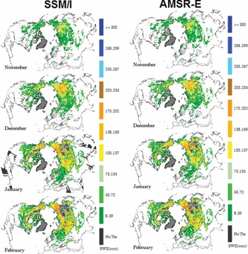
Figure 2.14 Northern Hemisphere monthly average snow water equivalent (SWE) derived from SSM/I (left) and AMSR-E (right), November 2003–February 2004
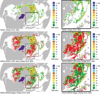
Figure 2.15 (a) shows Northern hemisphere snow water equivalent (SWE) map derived from NSIDC Global Monthly EASE-Grid SWE Climatology, with enlarged area in Northern Europe and Western Russia for October 24–31, 2003; (b) shows additional snow-covered area (red), determined from at least 25% of component MODIS CMG pixels indicating snow cover; (c) shows improvement in shallow snow SWE estimates by combining 89 GHz data with MODIS snow-covered area (select day w/ max diff 37 − 85 GHz)
Reference Gan, Kalinga and SinghGan et al. (2009) retrieved the SWE for the Red River basin of North Dakota and Minnesota using SSM/I, physiographic and atmospheric data by MCPN, a Projection Pursuit Regression (PPR) and a nonlinear regression. They used the airborne gamma-ray measurements of SWE as the observed SWE. They screened the SSM/I data for the presence of wet snow, large water bodies like lakes and rivers, and depth hoar. They found MCPN to produce encouraging results in both calibration and validation stages (R2 was about 0.9 for both calibration (C) and validation (V)), better than PPR (R2 was 0.86 for C and 0.62 for V), which in turn was better than the multivariate nonlinear regression at the calibration stage (R2 was 0.78 for C and 0.71 for V). MCPN is probably better than the linear and nonlinear regression counterparts because of its parallel computing structure and its ability to learn and generalize information from the SWE-SSM/I relationships.
Reference TakalaTakala et al. (2011) developed an algorithm assimilating synoptic snow depth data of weather stations with passive microwave radiometer data to produce a 30-year time-series of seasonal SWE for the NH, which was validated against independent SWE data from Russia, the former Soviet Union, Finland and Canada. The results show an overall strong performance in the SWE retrieved with root mean square errors below 40 mm when SWE <150 mm, but the retrieval uncertainty increases when SWE is above 150 mm. The SWE estimates obtained by this assimilation approach are better than SWE obtained from typical stand-alone retrieval algorithms shown above.
Active microwave data
In contrast to passive microwave data, active microwave data acquired by synthetic-aperture radar (SAR) sensors can attain much higher spatial resolutions. SWE can also be estimated using active microwave data such as the SIR-C/X-SAR data by Reference Shi and DozierShi and Dozier (2000), or possible future data from the dual-frequency (X-/Ku-band) synthetic aperture radar (SAR) satellite proposed by the Cold Land Processes Working Group (CLPWG) of NASA. Active and passive microwave sensors have different sensitivities to the same snowpack properties, and so they can provide complementary information. With improved resolution (about 10 km), passive microwave measurements can help supporting the high-resolution radar measurements, make linkages across process scales, and help relating future, dual-frequency SAR missions such as the Snow and Cold Land Process (SCLP) mission to the long-term microwave record of snow.
2.10 Snowmelt modeling
Spring snowmelt forms a major hydrological event of the year and it is the major source of fresh water for municipal and industrial water supply, irrigation, and hydropower generation over regions of mid- and upper latitudes. Globally more than one billion people depend on melting snow or glaciers for their primary water resource. The amount of snowmelt depends upon the energy available at the snow surface and the SWE present in the basin. An accurate estimate of the highly variable, basin to regional scale melt process is still a great challenge. This problem is more severe in open environments where blowing snow is a dominant winter phenomenon that prevents the computation of an accurate annual water balance. On the other hand, in a forest environment, it is also found that as canopy density increases, penetration of radiation and snowmelt rate decreases. However, under some conditions, snowmelt had been found to increase under dense canopy due to decreased terrestrial radiative losses (Reference Yamazaki and KondoYamazaki and Kondo, 1992). Under leafless deciduous canopies, the net radiation alone is a good predictor of snow ablation (Reference PricePrice, 1988) but it is not adequate to estimate snowmelt under the influence of canopy in the boreal forest (Reference Metcalfe and ButtleMetcalfe and Buttle, 1995).
The principles behind snowmelt modeling are first described below, then the intercomparisons of snowmelt models conducted in recent years are discussed. Snowmelt models developed for open and/or forest sites vary over a wide range of complexity, ranging from simple models such as the SNOW-17 of Reference AndersonAnderson (1976) which uses the degree-day method and a simple approach to consider canopy’s hindrance to snowfall, to land surface schemes in GCMs of intermediate complexity, for example, SSiB3 of Reference Xue, Sun, Kahan and JiaoXue et al. (2003), to complex canopy-atmosphere-soil models, for example, ACASA of Reference Pyles, Weare and PawuPyles et al. (2000). Modeling snow processes has been identified as an area of continuing weakness in global land surface models (Reference DirmeyerDirmeyer et al., 2006), because large discrepancies remain in albedo for forests under snowy conditions, due to difficulties in estimating the extent of masking of snow by vegetation (Reference Solomon, Qin, Manning, Chen, Marquis, Averyt, Tignor and MillerIPCC, 2007; Reference EsseryEssery et al., 2009).
Empirical snowmelt-runoff models
Empirical or statistical models (Equation 2.8) such as linear (all γi = 1, i = 1, 2, …, n) or nonlinear (at least one or more of γi ≠ 1, i = 1, 2, …, n) regressions based on SWE measured using snow pillows or snow course samplers at selected sites and/or baseflow measured for winter months such as November to March, as independent variables, for example, B1, B2, …, Bn, have been popularly used to forecast spring snowmelt of river basins. These models assume that under average snowpack conditions, empirical relationships derived between spring snowmelt runoff and measured snowpack data in the past are applicable in future years.
 (2.21)
Another statistical method for predicting spring snowmelt runoff is to relate SCA with spring snowmelt.
Degree-day or temperature index (TI) method
Many operational snowmelt runoff models use the degree day (temperature index) approach that estimates the snowmelt rate M (mm d−1) as the difference between the mean daily air temperature (Ta) and a melt-threshold or base temperature (Tthm) adjusted by some optimized melt factors mf in mm d−1 °C−1, and a depletion curve that relates how of the original snow cover remains versus mean areal extent of snow cover (e.g., WMO, 1986). mf depends on vegetation types, the slope and aspect of the land surface, percent of snow cover, time of the year and the climatic regime (Reference Frank and LeeFrank and Lee, 1966). So in applying Equation (2.22) to each basin zone, a different mf is usually used to reflect the vegetation characteristics and climate of each zone. The TI method has been widely used in operational snowmelt forecasting because by adjusting the degree-day, (Ta − Tthm), with an appropriate mf, it can approximately represent the daily energy supply for melting snowpack on a regional basis.
 (2.22)
In addition, mf has been found to vary seasonally, and tends to increase as the season progresses because of a decrease in snow albedo, and an increase in incoming solar radiation; in some cases the melt factor is allowed to vary through the melt season, such as a form of sinusoidal function in Equation 2.23,
 (2.23)
where mfmax and mfmin are the maximum and minimum melt rate, and n is the Julian date.
Even though the degree-day approach may work well in mid-latitude or temperate environments when there is a strong correlation between Ta and the dominant energy responsible for snowmelt, it does not adequately account for many climatic factors related to snowmelt. For example, Reference Male and GrangerMale and Granger (1981) showed that in open, non-forested areas the short wave radiation exchange is a dominant melt-producing energy flux, but it generally does not correlate well with air temperature. Moreover, the consideration of a uniform snow accumulation in the whole elevation range followed by a snowmelt process based on an assumed areal depletion curve is hardly imaginable in a mountain basin (Reference MartinecMartinec, 1980). Some newer models use satellite images to update its areal snow cover distribution and do not solely rely on an areal depletion curve. Examples of more widely used degree-day models are such as the NWSRFS (National Weather Service River Forecast System) (Reference AndersonAnderson, 1976), SRM (Snowmelt Runoff Model) (Reference Martinec, Rango, Roberts, Baumgartner and ApflMartinec et al., 1998), HBV (Swedish Meteorological and Hydrological Model) (Reference Bergström and SinghBergström, 1995; Reference Seibert and VisSeibert and Vis, 2012), and others.
Modified degree-day or modified temperature index (MTI) method
Reference Singh, Gan and GobenaSingh et al. (2005) introduced a modified degree-day method that includes the near-surface soil temperature (Tg) as an additional predictor,
 (2.24)
where mrf is an adjustment factor for mf so as to better capture the onset of initial snowmelt and is estimated from
 (2.25)
where β1, β2, β3, and ψ are model parameters derived through calibration (see Reference Singh, Gan and GobenaSingh et al., 2005). As a tangent function, mrf is relatively small when Tg < 0 °C, and reaches an upper limit of one when Tg ≥ 0 °C. The effect of mrf is “felt” mostly during the onset of snowmelt because its value approaches 1.0 when Tg approaches 0 °C. The desired rate of change of mrf can be achieved by adjusting the parameter ψ. Tr is a reference temperature computed as a weighted average of Tg and Ta,
 (2.26)
where χ is also a model parameter. The rationale for the proposed modification comes from past studies that pointed out the importance of Tg as an indicator of spring snowmelt (Reference Woo and ValverdeWoo and Valverde, 1982), as well as the analysis of data observed at the Paddle River Basin (PRB) in central Alberta by Reference Singh, Gan and GobenaSingh et al. (2005). Analysis of hourly data observed for 6 years during the spring season (March 1–April 30) at PRB shows that there is a significant correlation between net radiation (Rn) and Tg at daily time step. Moreover, the data revealed that Pearson’s correlation coefficient between Tg and Rn (ranging from 0.62 to 0.89) was mostly higher than that between Ta and Rn (ranging from 0.47 to 0.87). Since Rn generally dominates the energy balance during spring snowmelt in the Canadian Prairies (Reference ShookShook, 1995), adding Tg as another predictor should improve the performance of Equation 2.22.
Modeling snowmelt by energy balance method (EBM)
A more physically based snowmelt modeling approach is an one-dimensional (1-D) mass and energy balance model, such as the US Army Cold Regions Research and Engineering Laboratory (CRREL) model, SNTHERM developed by Reference JordanJordan (1991) for predicting snowpack properties and temperature profiles (Figure 2.16). SNTHERM calculates energy exchange at the surface and bottom of the snowpack, grain growth, densification and settlement, melting and liquid water flow, heat conduction and vapor diffusion, and solar absorption. The model’s surface boundary conditions require incoming solar and longwave radiation; wind speed, air temperature and humidity at some reference height; and precipitation. Lower boundary conditions include soil textural properties (currently clay or sand used as defaults), wetness and temperature profile.
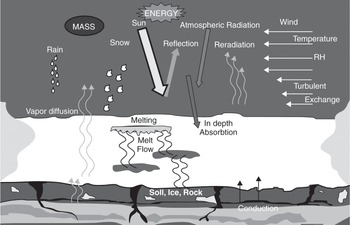
Figure 2.16 Energy fluxes considered in SNTHERM, a physically based 1-D energy balance model for snow and soil by Reference JordanJordon (1991)
SNTHERM accounts for changes in albedo due to grain growth, sun angle and cloud cover but it does not account for the decrease in effective albedo when the snow depth is shallow and when radiation penetrates through the snowpack to the underlying soil. It is expected that the snow albedo decreases exponentially to the soil albedo when the radiation penetrates through the snowpack to the underlying soil, and in a forest environment, the accumulation of forest litter could reduce snow albedo. In the energy balance approach, which is mostly considered in the vertical direction only, both the energy content of the snowpack plus a soil layer underneath that interacts thermally with the snowpack should be considered. This procedure provides a simple approximation of the effects of frozen ground, or snow falling on warm ground. The model output provides snow depth, profiles of snow temperature, water content, density, grain size, and surface fluxes of sensible heat and evaporation. Reference ShiShi et al. (2009) used SNTHERM to simulate the snow profiles of a 1,200-km transect of snow stratigraphy measured in Alaska. SNTHERM has been extensively tested for the prediction of temperature, snow depth, SWE, and snow-covered sea ice in sites such as the California Sierra Nevada (Reference MarksMark, 1988), Greenland (Reference Rowe, Kuiven and JordanRowe et al., 1995), the Canadian Boreal forest (Reference HardyHardy et al., 1998), the Arctic (Reference Jordan, Andreas and MakshtasJordan et al., 1999), Antarctic (Reference Andreas, Jordan and MakshtasAndreas et al., 2005), southern Finland (Reference Koivusalo and BurgesKoivusalo and Burges, 1996), and other Nordic environments (Reference KotlyakovLanglois et al., 2009).
A comparative study of three snow models with different complexities was carried out by Reference JinJin et al. (1999) to assess how a physically detailed snow model can improve snow modeling within general circulation models. The three models were (a) SNTHERM; (b) a simplified three-layer model, Snow–Atmosphere–Soil Transfer (SAST), which includes only the ice and liquid-water phases; and (c) the snow submodel of the Biosphere-Atmosphere-Transfer-Scheme (BATS), which calculates snowmelt from the energy budget and snow temperature by the force–restore method. SNTHERM gave the best match to observations with the SAST simulation being close. BATS captured the major processes in the upper layers of a snowpack where solar radiation is the main energy source and gave satisfactory seasonal results.
CROCUS is a model of the Centre d’Etudes de la Neige, Grenoble (Reference BrunBrun et al., 1992). It is a 1-D physical model that determines mass and energy balance for a snow cover and is used for operational avalanche forecasting. The snow cover is represented as a pile of layers parallel to the ground. Energy exchanges are projected orthogonally to the slope. The model describes the evolution of the internal state of the snow cover as a function of meteorological conditions. The variables describing the snow cover are temperature, density, liquid water content, and snow type of each layer. To match the natural layers, the thickness and number of layers are adjusted by the model. The model simulates the heat conduction, melting/refreezing of snow layers, settlement, metamorphism, and percolation. It simulates dry and wet snow metamorphism with experimental laws derived from laboratory data. Snow grains are characterized by their size and type. This allows an accurate albedo of the snow cover to be calculated.
Reference Bartelt and LehningBartelt and Lehning (2002) presented a 1-D physical model of the snowpack (SNOWPACK) with equations for heat transfer, water transport, vapor diffusion, and mechanical deformation. In their model, new snow, snow drift, and ablation are considered, and the snow layers are treated in terms of height, density, and microstructure (grain size, shale, and bonding). The model is used for avalanche warnings in Switzerland. Reference LangloisLanglois et al. (2009) simulated the SWE in southern Quebec using SNOWPACK, CROCUS, and SNTHERM models driven by local and reanalysis meteorological data, which are in agreement with ground measurements of SWE in winter seasons of 2004/2005, 2005/2006, and 2007/2008, with correlation coefficients ranging between 0.72 and 0.99.
One-dimensional vertical EBM
A 1-D energy balance snowmelt model developed by Reference Singh, Gan and GobenaSingh et al. (2009), which they refer to as SDSM-EBM, is briefly described. The model incorporates processes for snow interception by forest canopy, separate snowpack energy and mass balance for open and forested areas, separate water balance for liquid and ice phases, snow sublimation, compaction, refreezing, and so on. The snow interception capacity at different levels of canopy is estimated as a function of LAI, forest types (Reference Hardy and Hansen-BristowHardy and Hansen-Bistow, 1990), tree species, and prevailing forest structure (Reference Golding and SwansonGolding and Swanson, 1986). Reference PomeroyHedstrom and Pomeroy (1998) tested the snow interception model for the Canadian southern boreal forest, which Reference Singh, Gan and GobenaSingh et al. (2009) implemented in SDSM-EBM.
The transfer of energy at the snow surface and the snow/soil interface governs the snowmelt. The amount of energy available for melting snow is determined from the 1-D, energy equation (Equation 2.27) applied to a control volume of snow having upper and lower interfaces with air and ground, respectively. During melting, the snowpack is isothermal at 0 °C (
 = 0 °C) and the heat for snowmelt, Qo, can be calculated as
 (2.27)
where
Qn = Net radiation (short-wave and long-wave) absorbed by the snow,
Qh = Convective or turbulent sensible heat flux exchanged at the surface due to a difference in temperature at the snow-air interface,
Qe = Convective or turbulent latent heat exchanged at the surface due to vapor movement as a result of a difference in vapor pressure (evaporation, sublimation, condensation) at the snow-air interface,
Qg = Ground heat flux at snow-interface by conduction,
Qv = Advective heat of precipitation,
Qf = Energy released by freezing of liquid water content, and
Part of Qo may be used to overcome the cold content of the snowpack, Qcc (see Equation 2.37). All fluxes are computed in terms of W m−2 or older units such as langley per min. The net shortwave radiation (Qsn = Qsi − Qso) can either be measured by a net radiometer or by two pyrometers measuring the incoming short wave radiation (Qsi) and the reflected short wave radiation (Qso) which depends on the albedo of the snow-covered area, and the net longwave radiation (Qln = Qli − Qlo) can be similarly measured using two pyrgeometers with one inverted. By knowing the air temperature and the surface temperature of snowpack, and the emissivity of the atmospheric medium, it is also possible to estimate Qli and Qlo using the Stefan-Boltzmann’s constant and the blackbody theory.
 (2.28)
Qs can also be converted to Qsn [= Qs(1 − α)] as a function of the areal albedo of a partially ablated snow cover (α), which can be taken as the larger of that retrieved from satellite images such as that of NOAA-AVHRR or MODIS, or computed from
 (2.29)
where αsn is the snow albedo that can be estimated from an albedo decay function (Reference Riley, Israelsen and EgglestonRiley et al., 1972), αg is the albedo of the ground surface and Asn is the fraction of snow-covered area, which can be tracked using either a linear,
 , or a non-linear, parameterizing the SWE probability distribution based on the basin’s topography and vegetation in a dimensionless form,
 , depletion curve. SD (D) is the snow depth (SWE), and h (Dmax) is the depth (SWE) at which snow cover is complete (or the depth (SWE) below which bare patches start to emerge). In computing Asn,
 is replaced by
 . From snow data collected at the Paddle River Basin (PRB), Reference Singh, Gan and GobenaSingh et al. (2009) found that h ranges between 0.07 and 0.1 m as the cutoff for a partial snow cover. In forest-covered areas, αsn can be further modified to account for the effect of litter fall fraction (Reference HardyHardy et al., 1998).
Qs can also be estimated empirically (e.g., Reference BrasBras, 1990) but it is subjected to errors because of possible cloud cover effects and air pollution problems. Instead of measuring snow albedo, it can also be estimated from the age of the last snowfall since αsn declines with age and αsn ranges from about 0.9 or higher for freshly fallen snow to less than 0.4 for shallow, dirty, and wet snow. Snowpack albedo has also being related to the cumulative maximum air temperature (US Army Corps of Engineers, 1956), snow grain size, or snow surface density which tends to increase with time.
The other important components of energy balance are Qh, Qe and Qv. Qg, usually being the smallest, is often ignored. The sensible heat, Qh, is due to the turbulent flux of energy exchanged at the snow surface, as the result of a difference in temperature between air (Ta) and snow surface (Ts), in contrast to Qe that is caused by the vapor pressure difference between air and the snow surface. As a turbulent heat transport through convection (like Qe), Qh is affected by wind, such that
 (2.30)
where k2 = 0.00357 cm m1/3 hr day−1 oC−1 km−1, Po (Pa) is the standard (actual) atmospheric pressure,
 is the wind speed (m s−1), za and zb = heights where air temperature and wind speed are measured respectively, and lv ≈ 250 kJ kg−1. A simpler way to estimate Qh transported through convection is
 (2.31)
where ρa is the air density, Cp is the specific heat of air (1,004 J kg−1 oC−1), and Ch is a bulk transfer coefficient that depends on displacement, roughness height, and atmospheric stability. An even simpler expression to estimate Qh is
 (2.32)
where Bh is the bulk transfer coefficient that replaces ChρaCp given in Equation (2.31). In SDSM-EBM, Ts is computed using one of three simplified heat flow models, namely the force-restore method, the surface conductance method, and the Kondo and Yamazaki method (Reference Singh and GanSingh and Gan, 2005).
The latent heat flux (Qe) is the sum of surface sublimation/condensation (Qe,surf) and blowing snow sublimation (Qe,bss). When water vapor is transported to the snow surface, it changes phase to either liquid or solid, releasing Qe,surf at the snow surface,
 (2.33)
where E is the rate of vapor transfer, Ce the bulk transfer coefficient for water vapor, le is the latent heat of sublimation (2,836 kJ kg−1) or the latent heat of vaporization (2,501 kJ kg−1), ea and es are the actual and snow surface vapor pressure (assumed saturated at Ts) in Pascal, respectively, and Po is the standard atmospheric pressure at sea level (≈101.33 kPa). es is estimated as
 (2.34)
The bulk transfer coefficient under neutral condition is computed from Reference BrutsaertBrutsaert (1982),
 (2.35)
where κ is the von Karman constant, zr is the reference height, d0 is the zero displacement height and z0 is the roughness height. The model can be run assuming neutral conditions or one of three options, namely that of Reference Price and DunnePrice and Dunne (1976), Reference LouisLouis (1979), and Reference MorrisMorris (1989) can be used to adjust Ce.
If the precipitation is rainfall, there is positive advective heat Qv that contributes toward melting the snowpack, Qo, given as
 (2.36)
where R = intensity of rainfall in cm hr−1, T = temperature of rainfall in °C, and cs = specific heat (2.093 kJ kg−1 oC−1 for snow, 4.186 kJ kg−1 oC−1 for water).
The cold content of a snowpack is the heat required to raise the temperature of the snowpack to 0 °C, if the temperature of the snowpack, Tp, which can be different from the snowpack surface temperature Ts, is less than 0 °C.
 (2.37)
where ρp is the snowpack density, cs is the snowpack specific heat, D is the snowpack depth in cm, and Tp is the snowpack temperature in °C. If Dcc is the cold content expressed in terms of the equivalent depth of ice at 0 °C that can be melted to water at 0 °C,

In computing Qcc, the heat capacity of the entrapped air is neglected, and the snowpack temperature Tp may be assumed as Ts if no information is available. In other words, Tp is assumed to be independent of depth below snow surface (z).
After overcoming the cold content of the snowpack, Qcc, the depth of snowmelt, M, due to Qo acting for a time interval Δt, is then
 (2.39)
where ρw is the density of water and θ is the thermal quality of snow, which is the fraction of ice in a unit mass of wet snow, or the ratio of the heat necessary to produce a given amount of water from snow to the amount of heat needed to produce the same quantity of melt from pure ice at 0 °C. θ usually ranges between 0.95 and 0.97.
The total energy needed to melt a snowpack is QoΔt = ρpDlms + Qcc, where lms is the actual latent heat to melt the snowpack of depth D. If Q is the amount of energy needed to produce the same amount of melt from pure ice at 0 °C, such that Q = ρpDlfs then by definition, the thermal quality of snow, θ is given by
 (2.40)
In theory θ can also be estimated if we know the liquid water content (Wliq) of a snowpack since by knowing that we can calculate lms (Equation 2.7), which will be easier than trying to measure lms. Among various methods available to determine Wliq of a snowpack, a popular approach is to measure Wliq by a time-domain reflectometry because of the large difference in dielectric constant between water and ice (Reference SchneebeliSchneebeli et al., 1998).
Given the insulating effect of vegetation cover, Qg, the exchange of energy between the snowpack and the underlying ground by conduction is often ignored except where the ground is frozen, or in tundra. If Qg needs to be accounted for, it can be computed as
 (2.41)
where λg, the thermal conductivity of soil, is about 0.4–2.1 W m−1 °C−1 for unfrozen silt and clay, and Tg is the ground temperature that changes with elevation z.
Snowpack water balance
The water balance equations can be expressed in terms of water and ice at both canopy and ground levels as

Here, Wt+Δt accounts for both the addition of precipitation (Pr or Ps) during the time step and the change in water and ice mass due to Qe (sublimation or freezing) depending on whether
 is isothermal at zero or less than zero,
 (2.43)
 (2.44)
The net energy exchange in the snowpack (Q*) is then equal to
 (2.45)
If Q* < 0, the snowpack is losing energy to the atmosphere (cooling), and some liquid water (if available) may be re-frozen. The amount of energy released to the snowpack (positive value) by re-freezing liquid water is given by
 (2.46)
The resulting changes in the liquid and ice phases are given by
 (2.47)
 (2.48)
 (2.49)
The negative snowpack temperature,
 (associated with its cold content), is then updated from Equation (2.42). If Q* > 0, the snowpack is gaining energy from the atmosphere (heating), and in the process the negative
 will increase until it just reaches the isothermal condition (
 → 0). When
 becomes positive, it is set equal to zero and Qo is computed by Equation (2.46) and applied to Equation (2.47) and Equation (2.48) to compute the new liquid and ice components of SWE.
At each time step, the compaction of snowpack, Scomp is based on the present snowpack density ρsp (=Wt+Δt / SDt+Δt), maximum ρs,max, and a settlement constant, cs (Reference Riley, Israelsen and EgglestonRiley et al., 1972), as

The depth of snowpack after compaction is the difference between SD and Scomp. ρs,max and cs are manually calibrated such that the simulated SD matches the corresponding snow course data for a given land-use. The effect of rain compaction on snow is also based on Equation (2.50), where SDt replaces SDt+Δt when precipitation is in the form of rain.
During melt (positive Qo) and
 is isothermal at 0 °C, water is removed as meltwater (Mij) when the liquid phase increases beyond the current liquid water holding capacity (LWHC) of the snowpack at the expense of the ice phase, or Mij is held within the pack when snowmelt first appears at the bottom of the snowpack.
 (2.51)
where i is the sub-basin number and j is the land use type, and recommended values for LWHC, a function of snowpack properties and the presence of depth hoar, are 0.02W to 0.05W (US Army Corps of Engineers, 1956), and 0.05W for ρsp < 400 kg m−3 (Reference Riley, Israelsen and EgglestonRiley et al., 1972). As meltwater contributes runoff at the bottom of snowpack, the new
 ,
,
 (2.52)
The final SWE is computed from Equation (2.49). Routing the meltwater through the snowpack is usually neglected because the routing time for moderately deep snow covers is usually less than the hourly time step of the 1-D energy balance snowmelt model.
Reference Singh, Gan and GobenaSingh et al. (2009) tested the standard and modified temperature index methods, and the 1-D EBM on a small watershed called the Paddle River Basin (PRB) (53º 52′ N, 115º 32′ W), a sub-basin of the Mackenzie River basin, in a semi-distributed approach whereby PRB was divided into units that have similar drainage patterns identified from digital elevation model data. This semi-distributed approach provides a trade-off between modeling resolution, complexity and data availability (Reference Biftu and GanBiftu and Gan, 2001) so that the snowmelt (Mi) for sub-basin i and at each time step is the sum of melt from each land cover, weighted by its corresponding areal fraction ϕj as
 (2.53)
where n is the total number of land cover classes considered. They found that both EBM and MTI models show good agreements between their simulated and observed values of PRB of 2006/2007 based on ρs,max of 250 kg m−3 for the deciduous forest (DF) areas (Figure 2.17a) and the coniferous forest (CF) (Figure 2.17b), respectively. Apparently better simulations of the snow depth could be achieved by varying ρs,max with time, which is in line with the anticipated increase in snow density with time. ρs,max continues to change due to interaction of the snowpack with freshly fallen snow and settlement, and usually reaches the highest value at the end of snow accumulation period. When compared to the snow pillow data collected, EBM reproduced the snow accumulation between January 1, 2007 and March 13, 2007 almost perfectly. After March 13, the model overestimated snow accumulation and similarly lagged the ablation by about 2 days. On the other hand, MTI slightly overestimated snow accumulation up to the beginning of March and then reproduced the late season accumulation and ablation almost perfectly. Similarly, the time series of SWE estimated from the daily snow depth averaged from hourly automated snow depth measurements and the mean measured ρs from bi-weekly snow surveys conducted for the BERMS (Boreal Ecosystem Research and Monitoring Sites) sites located within the southern boreal forest of Saskatchewan for 2006/2007 shown in Figure 2.17c, and for 2007/2008 in Figure 2.17d, respectively, are compared with SWE retrieved by the GlobSnow project (Reference LuojusLuojus et al. 2010). Despite of snow interactions with mixed vegetation and relatively dense forest, the BERMS data generally compare well with the GlobSnow data.
Figure 2.17 Comparison of observed SWE and snow depth (SD) to those obtained by EBM (dashed line) and MTI (solid line) of a sub-basin of PRB for 2006/2007 for (a) the deciduous forest (DF) and (b) the coniferous forest (CF) with daily snow pillow data, respectively; and comparison of observed SWE for the BERMS sites located within the southern boreal forest of Saskatchewan for (c) 2006/2007 and (d) for 2007/2008, respectively with the GlobSnow data
As an energy balance model, EBM accounts for the Qcc explicitly but as an empirical model, MTI does not account for the Qcc of the snowpack and so occasional warm air masses occurring in the winter may cause MTI to over-simulate snowmelt runoff. This is the limitation of the temperature index (TI) approach, where without considering the effect of Tg, the model performance could be rather poor in both the calibration and the validation stages, as shown in Figure 2.17c, when the effect of Tg in the MTI model (Equation 2.23) was completely ignored by setting χ to 1 and ψ to 0, making it a standard TI model (Equation 2.21). In order to appreciate better the improvement achieved by introducing Tg and also to perform a fair comparison between TI and MTI, Reference Singh, Gan and GobenaSingh et al. (2009) re-calibrated the mf of TI (Equation 2.21) based on Ta only. It was necessary to use an artificially low mf for TI to perform well at the calibration stage (figure not shown), for example, mf of 0.04 mm hr−1 °C−1 for DF, which is a very low melt factor. However, the model performance decreased considerably when these mf values were used for all validation stages (Figure 2.17c). Apparently in a Prairie environment where the seasonal snow cover is shallow to moderately deep, where Tg is found to have a fairly strong correlation with net radiation (Qn), and the onset of major snowmelt usually happens when Tg approaches 0 °C, using both Tg and Ta in a temperature index approach (e.g., MTI) should generally lead to more accurate results than using Ta alone, which is much less data demanding compared to the EBM model.
Reference Singh, Gan and GobenaSingh et al. (2009) further assessed the three snowmelt models in terms of hourly simulated runoff at the outlet of the PRB within the framework of the semi-distributed hydrologic model DPHM-RS (Reference Biftu and GanBiftu and Gan, 2001). At the calibration stage (figure not shown), EBM (R2 = 0.85, and RMSE = 1.01) and MTI (R2 = 0.79, RMSE = 1.24) performed reasonably well even though in terms of the timing of peak flows, both EBM and MTI show a tendency to somewhat lag the peak flows observed. At the validation stage, they found the results to be less satisfactory (R2 = 0.5 for both EBM and MTI) partly because of errors in the lapse rate and gradient used to distribute point temperature and precipitation measurements to sub-basins, errors in the rating curve-discharge relationships due to icing, and the “regulatory” effects of beaver dams in PRB’s streamflow.
Even though the degree-day or temperature index (TI) approach has been a popular tool in modeling the spring snowmelt in temperate climates, it seems that either the data intensive, energy balance or the modified TI approach of Reference Singh, Gan and GobenaSingh et al. (2009) should be applied to watersheds of northern climates. More extensive research on modeling the snowmelt processes in the cryosphere using the MTI approach should be done since the energy balance approach is generally not practical because its data requirements are usually not met except in watersheds chosen for intensive research studies.
Most energy based snowmelt models consider energy balance in the vertical direction only which may not be sufficient in a mountainous watershed where the effects of terrain features can be important. A snowpack may receive radiation reflected from a surrounding slope or shielded from the incoming radiation by adjacent terrains. For example, if the diffused radiation from the atmosphere to a horizontal plane is QD, the diffused radiation received by a slope of inclination angle Ź from the atmosphere will be 0.5QDcos2Ź where 0.5cos2Ź is the sky-view factor (Reference Dewalle and RangoDeWalle and Rango, 2008). If there is an adjacent terrain of albedo α, the incoming shortwave radiation reflected by the adjacent terrain and received by this slope will be Qsiα(1 − 0.5cos2Ź).
The effects of forest cover on snowmelt processes can be approximately accounted for by estimating the amount of shortwave radiation penetrated through the canopy, which, similar to the interception of snow by canopy, is a function of the LAI. If the incoming short wave radiation is Qsi, then the amount of radiation reaching the snowpack becomes Qsiexp(−ξLAI) where ξ is the extinction coefficient for shortwave radiation in a forest. Values of ξ depend on the forest types, for example, Reference Baldocchi, Matt, Hutchison and McMillenBaldocchi et al. (1984); Reference Chen, Rich, Gower, Norman and PlummerChen et al., (1997). The incoming longwave radiation, Qli, for a snowpack under forest cover will be the weighted sum of incoming longwave radiation that penetrated through the overhead canopy and the longwave radiation emitted by the forest.
Two-dimensional energy balance approach
The energy balance model presented above and most if not all energy balance models do not directly account for the effects of the distribution of two-dimensional (2-D) patchy snowcover on the local advective energy of melt processes. This limits their application in a shallow snow cover (<60 cm) environment particularly in late melting periods when beside radiative fluxes, turbulent fluxes should also be accounted for. It has been found that the maximum snowmelt rate occurs when the land is only partially snow-covered, and often when it is slightly less than 60% (Reference Schmidt, Grise and PaceShook and Grey, 1997). Because of lower albedo, the bare ground absorbs a larger amount of solar radiation than the adjacent snow patches. The energy imbalance induces an advective, turbulent transfer of latent and sensible heat from the bare ground to snow patches, enhancing the melt rate. Since advective melting is the greatest along the leading edge of a snowfield, under constant climatic conditions, the melt rate of a patchy snow cover should be related to the perimeter of the patches (Reference ShookShook, 1993), or linearly relate the effective patch size for a regular pattern to the average patch size of a complex snow-cover pattern (Reference EsseryEssery et al., 2006).
Besides radiative, sensible and latent heat fluxes, there can be local advection (turbulent energy) due to large area of bare patches within a snow field, which may significantly alter the energy balance, and becomes increasingly important to melt as the snow cover dwindles. The proportion between radiation and turbulent energy sources to melt depend on the size of the snowfield. The smaller snowpatches will be dominated by turbulent melt throughout the season, or until they disappear. For large snowfields, melting is dominated by radiative melt early in the season and turbulent melt late in the season as they decrease in area (Reference Shook and GrayShook and Gray, 1997). Near the leading edge of an alpine snowfield, Reference Olyphant and IsardOlyphant and Isard (1988) found that advection may contribute more than 30 MJ m−2 d−1 of melt energy on a very windy day and more than 12 MJ m−2 d−1 on a relatively windless day. They also found that the corresponding advective energy at 1 km from the leading edge decreases to 5 and 2 MJ m−2 d−1 on windy and windless days, respectively. Further, the effects of wind on a snowpack are more pronounced on the windward than on the leeward slopes.
The sensible heat and latent heat fluxes are primarily related to wind speed, atmospheric stability, temperature and vapor pressure of air and snow surfaces, when they are considered as 1-D flux elements. However, near the edge of patchy snow cover, such simplification may not give good estimation and thus requires the use of a 2-D model that considers the development of the boundary layer beginning at the edge of the snowpack. A 2-D turbulent diffusion model, proposed by Reference WeismanWeisman (1977), considers this aspect of energy exchange when air flows over a snow cover. The model assumes a steady turbulent flow of warm moist air mass moving from a homogeneous surface onto a ripe snowpack (isothermal at 0 °C), no change in albedo over the snowpack and so no change of the radiation terms from point to point. Also the model assumes that albedo does not vary over the snowpack, and so Qn remains constant. This assumption implies that only Qe and Qh vary over the snowpack. The model, therefore, considers the 2-D aspect of Qe and Qh, and quantify the snowmelt M′, due to condensation or sublimation and sensible heat, as,
 (2.54)
The steady-state equations that describe the mean airflow over the snow are continuity, conservation of momentum, sensible heat and water vapor.
 (2.55)
 (2.56)
 (2.57)
 (2.58)
where u, w are mean wind components in the x and z directions, T is temperature, q is specific humidity, ρ is air density, cp is specific heat of air at constant pressure, and
 , H and V are the turbulent fluxes of momentum, sensible heat, and water vapor, respectively. The molecular diffusion, lateral and forward turbulent diffusion, and the pressure term in x-momentum equation have all been neglected. The problem of airflow over a sudden change in surface temperature and humidity has been solved using the mixing length theory. A vapor diffusion equation is included in the set of conservation equations and a vapor buoyancy term is included in the stability length.
Reference WeismanWeisman (1977) found that a stable atmospheric condition dampens the turbulent diffusion of fluxes, and the melt rate is at a maximum near the leading edge and decreases by one-third approximately 15–20 m from the leading edge. He provides an approximation for the advection of energy that relates the dimensionless melt energy at a point (
 ) and total average melt over the snowpack
 as a function of dimensionless horizontal downwind distance (
 ) and dimensionless snowpack fetch
 , respectively.
 (2.59)
 (2.60)
The constants a, b, c and d depend on the stability parameters, A*, which is associated with temperature change, and B*, which is associated with specific humidity change. The snow surface temperature Ts can be retrieved from NOAA-AVHRR, MODIS or Landsat-TM data. Once the dimensionless melt is known, it can be converted to dimensional melt energy M′ by multiplying
 by the energy gradient at the leading edge of the snowpack. Tables 2.2 and 2.3 list some typical values. The above equation underestimates the melt flux for values of
 less than 104, which comes out to be about 25 m from the leading edge for an average roughness of snow (0.002 m).
Table 2.3 Values of constants c and d (Reference WeismanWeisman, 1977)
| A* | B*=0 | B*=0 | B* = 0.001 | B* = 0.001 |
|---|---|---|---|---|
| C | d | c | d | |
| 0 | 0.516 | 0.110 | 0.317 | 0.106 |
| 0.0001 | 0.346 | 0.105 | 0.316 | 0.100 |
The stability parameters, A* is associated with temperature change and B* is associated with specific humidity change, given as
 (2.61)

where k = von Karman constant, 0.4, zo roughness height (m),
 = frictional velocity upwind of the leading edge of sow (m s−1), To = temperature of snow surface (0 °C),
 = temperature of soil surface upwind of leading edge (0 °C), qo= surface specific humidity at snow surface temperature (assume saturation) and
 = surface specific humidity at the soil surface temperature, upwind of leading edge. The knowledge of soil surface temperature upwind of the leading edge of the snow patch can also be obtained from the empirical equations for vapor pressure deficit and psychrometric equations.
Once the dimensionless melt is known, it can be converted to dimensional melt energy M′ by multiplying
 by the energy gradient at the leading edge of the snowpack.
 (2.63)
where ρ is air density (kg m−3), and cp is specific heat of air (J kg−1 °C−1).
Reference Olyphant and IsardOlyphant and Isard (1988) found that Equation (2.27) does not provide a good estimate near the leading edges of discontinuous melting snow surfaces where the advective heat contributes greatly to the energy balance of late-lying snow, and they introduced a modified version of Reference WeismanWeisman (1977)’s 2-D boundary layer model. The model pertains to a unit width of snow surface aligned with the prevailing wind. The horizontal pressure gradient is assumed to be negligible, as is the forward component of turbulent diffusion. Time derivatives have been added to the momentum and heat flux equations in an effort to simulate time-dependent responses to the diurnal variation of ambient forcing. The relevant boundary layer equations include one continuity and three conservation equations (momentum, sensible heat and latent heat). The estimation of fetch length, which fluctuates with the wind direction, and the irregular shape of snow patches can be attempted empirically. So far, there have been limited attempts at 2-D snowmelt modeling, which is predominantly 1-D.
Intercomparison of snowmelt models
Since the intercomparison project by the World Meteorological Organization (WMO) on snowmelt runoff models conducted in 1986, some other model intercomparison studies have been conducted, ranging from small scale, individual studies, to international effort, of which the latest and most comprehensive is the SnowMIP2 (Reference Rutter and EsseryRutter et al., 2009). Reference Singh, Gan and GobenaSingh et al. (2009), for example, compared three semi-distributed snowmelt models, namely, a temperature-Index or degree-day model based on air temperature (Ta), a modified temperature index model based on Ta and near ground-surface temperature (Tg), and an energy-balance model that considers liquid and ice phases separately. For the Canadian Prairies where snowpack is shallow to moderately deep, and winter is relatively severe, apparently the modified temperature index model based on Ta and Tg can perform comparably well with the more complex energy balance model, because the advantage of using both Ta and Tg is partly attributed to Tg showing a stronger correlation with solar radiation than Ta during the spring snowmelt season, and partly to the onset of major snowmelt which usually happens when Tg approaches 0 °C.
In the SnowMIP2 project, thirty-three snowpack models of varying complexity were compared across a wide range of hydrometeorological and forest canopy conditions, for up to two winter snow seasons applied to five northern sites in the NH: Alptal of Switzerland; Boreal Ecosystem Research and Monitoring Sites (BERMS) of Canada; Fraser of USA; Hitsujigaoka of Japan and Hyytiȁlȁ of Finland (see Figure 2.11). As expected, Reference Rutter and EsseryRutter et al. (2009) concluded that it is easier to model SWE at open than at forested sites, where precipitation phase and duration of air temperatures >0 °C are key factors to the divergence and convergence of modeled estimates of the sub-canopy snowpack, and more consistent results are found between open than forested sites (Figure 2.18). Furthermore, a model that estimates snowpack accurately at a forest site may not do well at an open site and vice versa. Calibrated models at forest sites perform better than uncalibrated models, though the benefits of calibration may not translate to subsequent years, nor to open conditions, which is expected since forests have large influences on snow dynamics and many recent models have included vegetation canopy (e.g., Reference Niu and YangNiu and Yang, 2004; Reference Bartlett, MacKay and VerseghyBartlett et al., 2006).
Reference ChenChen et al. (2014) evaluated the snowpack simulated by six LSMs against one year of SWE data at 112 SNOw TELemetry (SNOTEL) sites in the Colorado River Headwaters region and 4-year flux tower data at two AmeriFlux sites. While all models captured the key characteristics of the seasonal SWE evolution well at all SNOTEL sites, no single model was the best capturing the combined features of the peak SWE, the timing of peak SWE, and the length of snow season. The models responded differently to different forest coverage, and deficient in the treatment of snow albedo and its cascading effects on surface energy deficit, surface temperature, stability correction, and turbulent fluxes, for all models substantially overestimated (underestimated) radiative flux (heat flux). There are also significant intermodel differences in modeling snowmelt and sublimation efficiency, for models with high snow accumulation and melt rates were able to reproduce the observed seasonal evolution of SWE. It seems the parameterization of cascading effects of snow albedo and below-canopy turbulence and radiation transfer is critical to simulate the SWE and the winter land-atmosphere interactions correctly.

Figure 2.18 Observed SWE (black dots) and the average of thirty-three modeled estimates for (a) (gray line) of forest site at Hyytiȁlȁ (61° 51′ N, 24° 17′ E) of Finland (taken from Reference Rutter and EsseryRutter et al., 2009), and (b) (green line) of open and forest site at Alptal (47° 03′ N, 8° 48′ E) of Switzerland
An integrated approach to modeling snow accumulation and ablation processes
With the availability of geographical information systems (GIS), digital terrain elevation (DTED) data, snow products such as that of NOHRSC, re-analysis data, spatially distributed remotely sensed (RS) data to augment our limited ground-based, point observations, and an exponential growth in computing power, it will be desirable to integrate distributed, physically based snow accumulation and ablation processes with RS data, and ground measurements of snowpack to better model snowmelt processes. The idea is to progress from empiricism (e.g., degree-day method) to a discipline of applied science, and to model hydrological processes from measurable causative factors. The building and applications of distributed snow models depend largely on our ability to retrieve useful snow accumulation and snowmelt information of reasonable resolution from RS data in order to augment limited ground measurements.
Ideally, such distributed models should be developed in the direction of sub-grid parameterizations rather than the traditional quest for refining the resolution of small-scale parameterizations. This means finding a trade-off between the resolution of processes modeled, the types of data available and the information contained in the data, and the accuracy required. Otherwise, such models may be difficult to apply because of excessive data demand and the difficulty in obtaining the parameters required at all grid elements. On the other hand, some distributed snow models are based on rectangular or square grid elements of constant size without considering sub-grid parameterization, irrespective of the terrain features. This means that process descriptions may become “artificial,” since nature does not behave as a system of symmetrical grids placed side by side.
There have also been developments in land surface schemes using existing Surface Vegetation Atmosphere Transfer Schemes (SVATS), such as the Land Data Assimilation
Systems (LDAS) (http://ldas.gsfc.nasa.gov/) which are forced with gauged precipitation, RS data, radar precipitation, and output from numerical weather prediction models. Then in situ or remotely sensed measurements of LDAS storages (such as snow), water and energy fluxes will be used to validate and constrain the LDAS predictions using certain data assimilation techniques. However, one of the possible drawbacks of LDAS is the discretization of grids symmetrically without including sub-grid parameterization. Even with subgrid parameterizations in distributed models, ideally it may be more desirable to develop semi-distributed models that discretize river basins according to terrain characteristics, and that are designed to model snow, water, and energy dynamics with practical details under the forcing of fluxes and the influence of terrain and vegetation characteristics, in a framework that mimics nature as much as possible.
2.11 Recent observed changes in snowpack and snow cover
In spite of uncertainties associated with snow maps derived from passive microwave images, the detection of large scale changes to snowpack in higher latitude regions in relation to possible global warming is only possible through satellite images. Due to their effects on energy and moisture budgets, and surface temperature being highly dependent on snow cover, snow cover trends serve as key indicators of climate change (Reference Armstrong and BrunArmstrong and Brun, 2008). Observational records from satellites indicate that the annual SCA in the NH has been decreasing since 1960s due to increasing air temperature. The decline in seasonal snow cover is marked in spring and summer, but fall and winter snow cover has increased. The observed changes in the hemispheric snow cover correspond to warming and the feedback effects on the energy balance (Reference Barry, Cuff and GoudieBarry, 2009). Global-warming tends to affect winter temperatures, and in high latitudes, warmer winters may be snowier as a result of increased atmospheric moisture content.
Snowmelt in Greenland and Antarctic
About 20 years of SSM/I passive microwave data has been used to monitor the regional snowmelt of Greenland since 1988 (Reference TedescoTedesco, 2007; Reference TedescoTedesco et al., 2008). Defining a melting index (MI) as melting area multiplied by melting days, 2005 was the year with the highest MI, followed by 2002, 1998, 2004, and 2007. In 2007, areas higher than 2,000 m in southern Greenland experienced about 30 more days of melting than the study period of 1988–2007, and 53% higher MI than the average, even though overall Greenland had a MI about 20% higher than the average. In contrast, in 2008 northern Greenland experienced record melting, and they attributed record melting of snow in different parts of Greenland to warmer surface temperature.
Snow cover extent
Based on the 12-month running means, the monthly SCE over NH lands (including Greenland), Eurasia and NA for about 40 years (1966–2006) mainly show negative snow cover anomalies since the late 1980s, with the exception of 1996 and 2002 for NH and Eurasia, and 1997 for Eurasia and NA (Reference RobinsonRobinson, 2008). The SCE over NA has been shown to increase during autumn and early winter (November–January), but decrease over early spring (Reference Frei and RobinsonFrei and Robinson, 1999; Reference Dyer and MoteDyer and Mote, 2006), which indicates an earlier onset of the spring snowmelt. Reference Burn and KokeljCallaghan et al. (2011b) found Arctic snow cover showing different regional responses to climate warming and increasing winter precipitation that has characterized the Arctic climate in recent decades, with the largest and most rapid decreases in SWE and snow cover duration (SCD) observed over maritime regions of the Arctic with the highest precipitation amounts. Eurasian Arctic region has experienced larger declines in SCD (12.6 days), compared to the North American Arctic region (6.2 days) between 1982 and 2011 (Reference Barichivich, Briffa and MyneniBarichivich et al., 2013). Further, the North American sector of the Arctic exhibiting decreases in SCE and snow depth when in situ observations became available since 1950s, while widespread decreases in SCE are only apparent over Eurasia in the Arctic after 1980s, but snow depths are increasing in many regions of Eurasia. Warming and more frequent winter thaws are contributing to changes in snowpack structure.
Even though the SCE in January 2008 of 50.1 × 10⁶ km2 was the largest recorded SCE for January in the last 40 years, the 2008 annual SCE over NH lands averaged 24.4 × 10⁶ km2, which is 1.1 million km2 less than the 39-year average, putting 2008 as the fourth least extensive snow cover on record, and the 12-month running means ran below the long-term average throughout 2008, following the generally lower than average extents in 2007. The SCE in January has been declining consistently since the notable minimum in the late 1980s and early 1990s over Eurasia, even though in North America, the SCE anomalies have somewhat rebounded over the course of 2008 from a 2005–2007 minimum. From a snow model that generated monthly SCE of NH from 1905 to 2002, Reference McCabe and WolockMcCabe and Wolock (2010) found a substantial decrease in the March SCE of NH since 1970s attributed to an increase in the mean winter temperature and a contraction of the circumpolar vortex and a poleward movement of storm tracks, which resulted in decreased precipitation (and snow) in the low- to mid-latitudes and an increase in precipitation (and snow) in high latitudes.
Are these generally negative snow cover anomalies since the late 1980s an indication of the warming trends detected for North America, Europe, and Asia in NH? From the Mann–Kendall’s trend analysis of SCE of NH over 1972–2006, Reference Déry and BrownDery and Brown (2007) found significant declines in SCE during spring over North America and Eurasia, with lesser declines during winter and evidence of a poleward amplification of decreasing SCE trends during spring over Eurasia and North America, which is consistent with an enhanced snow-albedo feedback over northern latitudes that act to reinforce an initial anomaly in the cryospheric system.
In recent years, the fraction of precipitation in mid- and higher-latitude regions falling as snow has decreased, the fall accumulation has been occurring later while the spring ablation earlier, and the northern hemisphere’s (NH) SCE and snow depth have decreased, which would have significant socioeconomic consequences as more than one-sixth of the world’s population depend on meltwater for their water supply. Climate warming has been the dominant factor in the observed decrease in winter SCE and earlier spring ablation over North America (NA) (Reference Dyer and MoteDyer and Mote, 2006), given air temperature anomalies over NH’s mid-latitude land areas has been shown to explain about 50% of the observed variability in SCE (Reference Brown and RobinsonBrown and Robinson, 2011).
Numerous observations have shown that the SCE of NH has been decreasing rapidly in recent decades, especially in spring, and in warmer locations where SCE are closely linked to temperature variability, for example, March–April SCE of NH is decreasing at 3.4%±1.1% per decade (1979–2005) (Reference Brown and RobinsonBrown and Robinson, 2011; Reference Hernández-Henríquez, Déry and DerksenHernández-Henríquez et al., 2015). Over 1967–2012, the annual mean SCE has significantly decreased, with the largest change, −53% [−40 to −66%], occurred in June. Over 1922–2012, a much smaller 7% [4.5–9.5%] decline for March–April was found. Majority of climate stations show decreasing trends, and stations at lower elevation or higher average temperature were the most liable to show a decrease.
The satellite-based visible SCE of National Oceanic and Atmospheric Administration (NOAA) climate data record (CDR) developed from weekly Northern Hemisphere SCE data span from October 4, 1966 to the present. Satellite data incorporated into the NH SCE CDR at various starting dates include platforms of the Environmental Science Services Administration (ESSA) series, NOAA Polar-orbiting Operational Environmental Satellites (POES), NOAA Geostationary Operational Environmental Satellites (GOES), the Defense Meteorological Satellite Program (DMSP) series, the Meteosat series, Geostationary Meteorological Satellites (GMS), Aqua, Terra, and the Multi-functional Transport Satellites (MTSAT) (Reference Estilow, Young and RobinsonEstilow et al., 2015). Starting in June 1999 the CDR is completely derived using the Interactive Multisensor Snow and Ice Mapping System (IMS) involving a diverse set of products: satellite imagery, snow and ice analysis maps, National Centers for Environmental Prediction (NCEP) model data, and surface observations, and improved discrimination between snow and cloud covers. With an 89 × 89 Cartesian grid laid over an NH polar stereographic projection and a cell size of 190.6 km × 190.6 km, cell areas range from ~10,700 km2 near the Equator to ~41,800 km2 near the pole.
Despite of many up and down cycles in snowfall that had occurred over the NH in last five decades, Figure 2.19 of the Rutgers University Snow Lab based on this CDR data set, the NH SCE exhibits an overall increasing trend since the late 1980s, in contrast to the overall decreasing trend observed between late 1960s and 1980s. The increasing trend in the SCE of the NH observed in the last three decades are attributed to increasing SCE in the Fall and winter seasons, especially the Fall season, which together had offset the overall decreasing trend in the spring SCE of the NH shown in Figure 2.19d. Trend estimates for annual precipitation of the 1951–2008 time series of CRU TS 3.10.01 (updated from Reference Mitchell and JonesMitchell and Jones, 2005) are 5.82 ± 2.72 and 1.13 ± 2.01, for GHCN V2 (updated through 2011; Reference VoseVose et al., 1992) are 4.52 ± 2.64 and 1.39 ± 1.98, and for GPCC V6 (Reference BeckerBecker et al., 2013) are 2.69 ± 2.54 and 1.50 ± 1.93 mm yr−1, for both latitudinal bands 30° N–60° N and 60° N–90° N, respectively (Reference HartmannHartmann et al., 2013). Even though confidence in precipitation change is medium for the years after 1950 because of insufficient data, the non-significant positive annual precipitation trends over both latitudinal bands of the NH should have contributed to increasing trends in the Fall and Winter SCE of NH of the last five decades. However, likely because of more rainfall than snowfall in spring and earlier onset of spring snowmelt, the Spring SCE of NH generally show decreasing trends despite of positive annual precipitation trends at latitudinal bands north of 30° N.

Figure 2.19 (a) Twelve-month running anomalies of monthly snow extent plotted on the seventh month using values from November 1966 to December 2018 for NH (https://climate.rutgers.edu/snowcover/chart_anom.php?ui_set=0&ui_region=nhland&ui), and seasonal snow cover extent of NH for (b) Fall, (c) Winter, and (d) Spring. The mean 1981–2010 SCE for the NH in Fall, Winter, and Spring are 18,912, 45,480, and 29,788 km2, respectively
Snow water equivalent
SWE of snowpacks, the depth of liquid water produced by a snowpack after complete melting, can be estimated from in situ depth (d) and density (ρs) in kg m−3 measurements, SWE = d(ρs/ρw), where the density of water ρw is about 1,000 kg m−3. So far passive microwave radiometry is the only spaceborne technique proven useful in extracting SWE data (Reference Walker and SilisWalker and Silis, 2002). SWE has been estimated from the brightness temperature (TB) of microwave frequency and polarization (H or V) of the TIROS-N sensor, the Scanning Multichannel Microwave Radiometer (SMMR) from the Nimbus 7 satellite with data between October 25, 1978 to August 20, 1987; the Special Sensor Microwave/Imager (SSM/I) data from the Defense Meteorological Satellite Program (DMSP) satellite with data available since September 7, 1987 (Reference Armstrong, Brodzik, Savoie and KnowlesArmstrong et al., 2006), and succeeded by the Special Sensor Microwave Imager/Sounder (SSMIS) in 2005, and the Advanced Microwave Scanning Radiometer‐Earth Observing System (AMSR-E) data from the Aqua satellite with data available between 2002 and 2011 or the Advanced Microwave Scanning Radiometer 2 (AMSR2) on the JAXA GCOM W1 spacecraft, launched May 18, 2012 and is still operating. Limitations to such SWE data are a coarse resolution (typically 25 km), underestimated in forests which mask the snow cover and vegetation suppresses the scattering signal, as does liquid water (wet snow). From retrievals of SMMR-SWE over Canada, Reference Dong, Walker and HouserDong et al. (2005) concluded that for practical applications, the uncertainty of such SWE data is acceptable for regions more than 200 km away from large open water bodies, daytime air temperatures lower than 2 °C, and SWE values are above 100 mm.
Reference MeisterMote et al. (2005) detected widespread declines in modeled April 1 SWE over the Western United States and Canada between 1950 and 1997. Reference Gan, Barry, Gobena and RajagopalanGan et al. (2013) detected significant decreasing trends in SWE in NA over 1979–2007, which are more extensive in Canada than in the United States where such decreasing trends are mainly found along the Rocky Mountains. However, because of uncertainties associated with SWE data retrieved from passive microwave data, results obtained for mountainous or forested areas of NA, the tundra in Arctic Canada with many frozen lakes or snow packs that consist of depth hoar and wind slab, should be treated with caution. To assess the possible impact of climatic change to the snowpack of North America, Reference Gan, Barry, Gobena and RajagopalanGan et al. (2013) analyzed the trends of temperature and precipitation data and then the SWE-air temperature and SWE-precipitation relationships. Using the gridded, 2-m air temperature data of the North American Regional Reanalysis (NARR) (Reference MesingerMesinger et al., 2006) and that of the University of Delaware (Reference Willmott and RobesonWillmott and Robeson, 1995), they detected statistically significant temperature trends for 1979–2007 (January–April) mainly in the southern states of USA. They also detected significant decreasing precipitation trends from the University of Delaware and the NARR data but there are limited agreements between the locations of significant decreasing precipitation trends and significant decreasing SWE trends. However, extensive areas of negative correlations between SWE and temperature exist both across the United States and Canada, and the distribution of these areas of negative correlation closely follows the areas of the decreasing trends detected from the SWE data, which for Canada is mainly east of the Canadian Rocky Mountains, while for the United States is mainly on the American Rocky. Apparently, extensive decreasing trends in SWE data of passive microwave detected in Canada and parts of USA are caused more by increasing temperatures than by decreasing precipitation. Higher air temperature means more rainfall and less snowfall especially in areas and seasons where the average air temperature is close to 0 °C, earlier onset of spring snowmelt, and generally less snowpack.
From SWE estimated from satellite measurements for October to April over 1979–2007 in NA, Reference Gan, Barry, Gobena and RajagopalanGan et al. (2013) found that about 25–30% of the pixels covered with snow showed statistically significant negative trends, compared with 5–10% that showed increasing trends. The overall mean trend magnitudes estimated are about −0.4 to −0.5 mm a−1 which means the overall SWE of NA had decreased by about 10–13 mm or possibly more, or in terms of snow depth could range from about 4 to 13 cm (depending on the snow density) over 1979–2007. The detected changes should have significant impacts on the spring snowmelt of, say, the Canadian Prairies and the Washington Cascades. Using a combination of satellite data, in situ data and land surface model simulations, Reference Park, Yabuki and OhataPark et al. (2012) found negative trends in snow depth more pronounced in North America than in Eurasia between 1948 and 2006. Reference Dyer and MoteDyer and Mote (2006) found significant (>1 cm yr−1) negative regional snow depth trends in central Canada along a southeast line from the Yukon Territory to the Great Lakes using in situ snow depth data for 1960–2000 for North America.
Global Cryosphere Watch (2015) has compiled a comprehensive snow data set from passive-microwave, in situ, and analysis/reanalysis products for non-alpine regions of the NH. The data set at 25 km resolution is available at daily, weekly and monthly time steps since 1979. By combining different data sources, GlobSnow is probably better than SWE data derived from stand-alone remote sensing data sets (Reference Frei, Tedesco, Lee, Foster, Hall, Kelly and RobinsonFrei et al., 2012).
Based on the non-parametric Mann–Kendall test at 0.05 significant levels, more snow-covered pixels of the monthly GlobSnow SWE data set of NH for November–April (1988–2017) show decreasing than increasing trends (Figure 2.20). From the total number of snow-covered pixels analyzed, up to 15.5% (7.7%) of the pixels show statistically significant decreasing (increasing) trends. December has the largest SCE and the greatest percentage of statistically significant decreasing trends, of which the majority are located north of 55° latitude. April exhibits the greatest percentage of statistically significant positive trends and most of these pixels are located in Asia.

Figure 2.20 Northern Hemisphere monthly snow cover for December–March of GlobSnow SWE data set of 1988–2017 that exhibit increasing (red) and decreasing (black) trends statistically significant at the 0.05 level using Mann–Kendall test
Figure 2.21 shows spatial distributions of grids of the Northern Hemisphere with significant SWE (5-day averages) trends at p < 0.05 significant level over 1988–2017 using the Mann–Kendall test. There are more statistically significant negative than positive SWE trends especially across Canada, the high Arctic, and Europe, with scatterered positive trends in Russia.

Figure 2.21 Spatial distributions of grids of the Northern Hemisphere GlobSnow data set with significant SWE (5-day averages) trends at p < 0.05 significant level over December–March of 1988–2017 using the Mann–Kendall test, with more statistically significant negative than positive SWE trends especially across Canada, the high Arctic, and Europe, while scatted positive trends in Russia
As expected, based on the Mann–Kendall’s test applied to the ERA-Interim reanalysis data, Figure 2.22 shows predominantly warming trends over the Northern Hemisphere in the last 30 years (1988–2017). On the other hand, some scattered cooling trends are still detected in the northern Pacific Ocean in January and March, over some eastern parts of Siberia in February, and a small part of the north Atlantic Ocean in March.

Figure 2.22 The spatial distribution of grids with statistically significant (p < 0.05) temperature Pentad (5-day averages) trends by the Mann–Kendall test in the Northern Hemisphere based on the 1988–2017 ERA-Interim reanalysis temperature data
The Spearman’s rank correlation between SWE and air temperature across the Northern Hemisphere is predominantly negative, which is expected because under the effect of climate warming, there should be an overall less snowpack partly attributed to more rainfall than snowfall, if the total precipitation will remain unchanged or even higher (Figure 2.23).

Figure 2.23 Spatial distributions of grids of the Northern Hemisphere with significant Spearman’s rank correlation between SWE and air temperature over 1988–2017 at p < 0.05 significant level
The Self Organizing Map (SOM) (Kohonen, 2001) is an artificial neural network developed to uncover an underlying structure in a data set through an unsupervised learning to produce a 2-D array of nodes, called a map, that are organized in such a way that similar items are placed close to each other. By applying the SOM and K-means clustering analysis, Northern Hemisphere grids were grouped into 20 different clusters based on the SWE niveograph of November–March for 1988–2017, for example, one grid can be assigned to a different cluster in different years. Figure 2.24 shows that grids in snow-dominated areas of Canada, Siberia, and northern Europe are generally assigned to more clusters (up to 20) than other regions of NH that also experience snowfall.

Figure 2.24 (a) Number of different clusters derived from the SOM and K-means clustering analysis that each grid in Northern Hemisphere is assigned over 1988–2017, and an example of (b) the SWE in boxplots for all grids of NH assigned to Cluster #5
Figure 2.25 shows some limited statistically significant Spearman’s rank correlation between SWE of the Northern Hemisphere and large-scale climate anomalies such as AO, PNA, NAO, and PDO, respectively. There are more negative (black) than positive (red) correlation especially between PNA and SWE, which means less snowpack during the warm than the cold phase of PNA. For example, in western Canada, Reference Gan, Gobena and WangGan et al. (2007) show that El Niño (La Niña) leads to a 14% decrease (20% increase) in the mean winter precipitation, strong positive (negative) PNA leads to a 12% decrease (9% increase) in mean winter precipitation, and PDO is associated with an 8% decrease (9% increase) in mean winter precipitation. The detected teleconnections could occur at interannual or interdecadal levels depending on the climate anomaly, and their strength changes in time and space.

Figure 2.25 The spatial distribution of grids with significant (p < 0.05) positive (red) and negative (black) Spearman’s rank correlation between cluster areas, AO, PNA, NAO, and PDO, respectively
Climate indices significantly correlated with any of the first four PCs of the SWE of NH at 0.05 significance level are shown in Table 2.4. Apparently AO, NAO and PNA exert a stronger influence on the snowpack of the NH between January and April. PC1 is more strongly correlated with AO and NAO, while PDO and PNA are more correlated with PC2 to PC4 in some months. Therefore, some of the observed changes in SWE are partly attributed to the influence of large-scale climate anomalies but climate warming has undoubtedly played a bigger role, especially in the detected negative trends of SWE of NH.
Table 2.4 Climate indices statistically significantly correlated to PC1 to PC4 of November–April 1979–2014 SWE of Northern Hemisphere
| Nov | Dec | Jan | Feb | Mar | Apr | |
|---|---|---|---|---|---|---|
| PC1 | AO, NAO, PNA | AO, NAO | AO, NAO | AO | ||
| PC2 | PDO | PDO | PNA | PNA | ||
| PC3 | PDO | AO | PNA | PDO | ||
| PC4 | PNA | SOI | PDO |
Reference Wu, Che, Li, Wang and YangWu et al. (2018) found slower snowmelt rates over the entire NH over 1980–2017, but with higher ablation rates in locations with large SWE, because of the reduction of SWE in deep snowpack regions. However, moderate and high snow ablation rates show a decreasing trend. Reference Kapnick and HallKapnick and Hall (2012) detected significant losses of spring mountain snowpack at western United States over past several decades. For Canada, there has been extensive decreasing snow depths and snow cover duration and extent since the mid-1970s, with the largest declines in western Canada and proportionally greater changes later in winter and spring (Reference DeBeer, Wheater, Carey and ChunDeBeer et al., 2016). Reference Berghuijs, Woods and HrachowitzBerghuijs et al. (2014) show that in conterminous USA, catchments with a higher fraction of precipitation falling as snow tends to have higher mean streamflow, which is likely to decrease in catchments that experience significant reductions in the fraction of precipitation falling as snow because of a warmer climate.
Most studies also show negative trends in snow depth and snow duration over past decades in the mountain cryosphere of Europe (Reference Beniston, Farinotti, Stoffel, Andreassen, Coppola and EckertBeniston et al., 2018), with less pronounced changes at high elevations (Reference Terzago, Fratianni and CremoniniTerzago et al., 2013). Spring SWE shows a decreasing trend in Alps (Reference Marty, Tilg and JonasMarty et al., 2017). However, there were positive trends of maximum snow depth and SWE in higher and colder parts of the Fennoscandian Mountains although it turns out to be negative trends in recent years (Reference Kivinen and RasmusKivinen and Rasmus, 2015). Reference Matti, Dahlke, Dieppois, Lawler and LyonMatti et al. (2017) show that the flood seasonality for snowmelt‐dominated Scandinavian catchments have changed over the twentieth century with statistically significant decreasing (increasing) trends in summer (winter and spring) maximum and mean daily flows in some catchments. Changes in annual flood occurrences generally point toward a shift from snowmelt‐dominated to rainfall‐dominated flow regimes in some regions, with flood peaks due to spring snowmelt consistently occurring earlier, often at the expense of the much needed summer streamflow for growing crops (Reference Kerkhoven and GanKerkhoven and Gan, 2011).
There are other cryospheric observations also support the effect of a warmer climate in the recent past. For example, the number of snow days in Switzerland decreased abruptly at the end of the 1980s. Reference MartyMarty (2008) found that records at 34 long-term stations between 200 m and 1,800 m asl for 1948–2007 show an unprecedented series of low winter snow in the last 20 years. The abrupt change in 1988 resulted in a loss of 20–60% of the total number of snow days with no clear trend since then. The decrease is shown to be correlated with an increase in winter temperatures.
SCE over North America has been shown to increase during autumn and early winter (November-January), although it also decreased in early spring (Reference Frei and RobinsonFrei and Robinson, 1999; Reference Dyer and MoteDyer and Mote, 2006), which indicates an earlier onset of the spring snowmelt. Some parts of the Canadian Arctic stretching from western Hudson’s Bay to the North Slope of Alaska shows a persistent pattern of high SWE (Reference Armstrong and BrodzikArmstrong and Brodzik, 2002; Reference Andreadis and LettenmaierAndreadi and Lettenmaier, 2006). However, as noted earlier, SWE data derived from passive microwave for the tundra in Arctic Canada should be treated with caution (Reference DerksenDerksen et al., 2009). Less snowfall has been observed in the lower Missouri River Basin (Reference BensonBerger et al., 2002) and in New England (Reference HuntingtonHuntington et al., 2004).
Reference MoteMote et al. (2005) found evidence of declining snowpack in the western United States, except in the southern Sierra Nevada. Reference Bedford and DouglassBedford and Douglass (2008) analyzed daily SWE from 28 SNOTEL stations in the Great Salt Lake Basin for 1982–2007. They found an advance of about 15 days in the date of peak SWE as well as (less robust) evidence of a decrease in peak and April 1 SWE amounts.
Through three spring indicators – lilacs, honeysuckles, and streamflow – Reference CayanCayan et al. (2001) found earlier onset of the spring season by up to three weeks in the western North America since the 1970s. By simulating the snow energy balance to climatic changes projected by nine regional climate models to the end of the twenty-first century in the Pyrenees, Moreno et al. (2008) concluded that the most significant changes to future snowpack processes are related to temperature. Reference TedescoTedesco (2007) concluded that record melting of snow in southern Greenland in 2007 was caused by higher surface temperature. The above documented observations about the cryosphere agree with the enhanced increasing trends of surface air temperature anomaly changes over other continents, especially enhanced temperature trends occurred in the last several decades since 1960s reported by IPCC (2013) (see Figure 2.26 adapted from Reference Jones, Stott and ChristidisJones et al., 2013). In Figure 2.26, multi-model means are shown as thick lines, and 5–95% ranges shown as thin light lines, and as black lines for HadCRUT4. Mean temperatures are shown for Antarctica and six continental regions. Temperatures are shown with respect to 1880–1919 for all regions apart from Antarctica where temperatures are shown with respect to 1950–2010.

Figure 2.26 Global, land, ocean, and continental annual mean temperatures anomaly with respect to 1880–1919 for CMIP3 and CMIP5 historical (red) and historicalNat (blue) simulations, and Hadley Centre/Climatic Research Unit gridded surface temperature data set 4 (HadCRUT4, black). Weighted model means shown as thick dark lines and 5–95% ranges shown as shaded areas