1. Introduction
Water is a vital resource on the planet and an indispensable input in crop production and almost every other activity. At the same time, agriculture represents the primary water user, mainly for irrigation, and has a central role in sustaining the growth of rural areas. As the world population grows and the total demand for food increases, the rivalry from other economic activities surges, and as a consequence, the water availability for crop production, in many regions, decreases [
1,
2]. Therefore, water conservation in agriculture attracts ever-increasing attention under the pressure of climate change and intense competition for the limited freshwater resources between the various users, especially in semi-arid and arid regions [
3,
4,
5,
6]. Additionally, the importance of water management practices to conserve freshwater ecosystems and biodiversity [
7] highlights the complexity of such an endeavour. In this framework, the sustainable management of water resources is a crucial step in preserving not only agricultural production, but the vast majority of activities that sustain contemporary societies [
8].
However, the lack of policy initiatives and widespread use of inefficient irrigation practices present significant threats for water resources and food security [
9]. Indicatively, extensive research on effective agricultural water management practices in the last decades includes research on new irrigation technologies, deficit irrigation, cultivation of drought-resistant crops and optimisation of crop patterns avoiding water-intensive crops [
9,
10,
11,
12,
13]. Recent technological developments in sensors, communication and automation technologies also provide a sound basis for efficient irrigation management based on environmental measurements such as soil moisture, evapotranspiration or crop stress [
3,
4,
14,
15].
Agriculture, therefore, is an essential driving force in the management of water use. Therefore, it has a central role in the Rural Development Programme (RDP) of the European Union and the Common Agricultural Policy (CAP) objective of “ensuring sustainable management of natural resources and climate action”. Progressively, the CAP has embraced environmental goals [
16,
17]. These goals, undoubtedly, are the primary source of funding and the critical form of public intervention influencing natural resources and environmental management [
18,
19]. The primary policy tool in pursuing CAPs’ environmental objectives are the Agri-Environment Measures (AEMs) [
18]. The AEMs target water savings directly or indirectly. For example, the AEMs which attempt to control the use of nutrients also target irrigation water savings. These measures set aside a proportion of the farm’s land and reduce the use of nutrients and water on the rest. As a result, such AEMs alter the agricultural land use pattern in the areas where they operate. At the same time, other measures aiming at securing crop production and increasing competitiveness align with the overall environmental objectives [
20,
21].
The evaluation of rural development policy holds a key role in safeguarding RDP efficiency in achieving the CAP objectives. Evaluation makes use of specific questions (Common Evaluation Questions—CEQ) and impacts indicators that are common among all EU member states. CEQs and impact indicators are part of the EU’s Common Monitoring and Evaluation Framework (CMEF). Monitoring and evaluation are indispensable to adaptive policy design and management [
22]. Proper indicators play a critical role in policy evaluation as well as in supporting actors in making well-informed decisions based on timely, contextualised, and actionable information [
1,
23]. In this context, academic research attempts to elaborate on robust indicators that will unravel the impact of policy measures on issues related to water use. These issues refer to total water abstraction, water-use efficiency in terms of “crop to drop”, and the water footprint of production. As such, addressing them is highly essential for decision-makers in water-for-food governance from the local to the global level [
24,
25,
26].
The leading impact indicator related to water is I.10—“Water abstraction in agriculture” and its complementary result indicator is R.13—“Increase in efficiency of water use in agriculture in RDP supported projects”. The related CEQ is “To what extent has the RDP contributed to the CAP objective of ensuring sustainable management of natural resources and climate action?” To this end, the European Commission (EC) provided a set of detailed, nonbinding guidelines for “Assessing RDP achievements and impacts in 2019” through the European Evaluation Helpdesk for Rural Development [
27]. The guidelines present several alternative methodologies which can fulfil the evaluation quality criteria of rigorousness, reliability, robustness, validity, transparency, credibility, practicability and cost-effectiveness.
The indicator I.10—“Water abstraction in agriculture” refers to the volume of surface and groundwater applied to soils for irrigation purposes. According to the definition adopted in Regulations (EC) No. 1166/2008 and (EC) No. 1200/2009 on farm structure surveys and the survey on agricultural production methods correspondingly: “the volume of water cubic metres used for irrigation per year is defined as the volume of water that has been used for irrigation on the holding during the 12 months prior to the reference date of the survey, regardless of the source (VIII. Irrigation, Annex II of Commission Regulation (EC) No 1200/2009). The estimation may be produced by means of a model (art. 11 of Council Regulation (EC) No 1166/2008)”.
According to the guidelines [
27], the most appropriate data source so far is the “Survey on Agricultural Production Methods” provided by Eurostat; however, relevant data are available only for 2010. Besides, the data sources used in many countries to make these estimations are unclear, given the absence of appropriate monitoring infrastructure in local water distribution authorities or metering devices on individual farms. The quality of the information collected will improve in the future since this is an “ex-ante conditionality” for funding, i.e., a precondition for providing funds. Hence, at this moment, the use of models that can estimate the volume of water used in agriculture based on agricultural land use recorded by Integrated Administration and Control System (IACS), meteorological data and annual crop statistics seems to be the most suitable methodology for countries facing data sparseness. Models are widely used in every aspect of planning and management of water resources in agriculture [
5,
28,
29,
30,
31,
32] as well as in evaluating various economic and environmental impacts of RDP effects [
8,
17,
18,
33,
34,
35].
A hydrological model is a computer-based simplified representation of a real-world hydro system that enables researchers to understand, predict and manage water resources. There are several types of models according to the application, the modelled processes, the method and the time and space scales. Specific purposes and specific scales necessitate the use of various modelling approaches [
36]. Also, advances in hydrological knowledge and the increasing abundance of computer power facilitate the development of more sophisticated and more efficient models. Hydrological models are characterised as lumped, distributed and semi-distributed, according to the spatial scale in which they represent the hydrological processes. Lumped models describe a watershed as a single entity and simulate storages and fluxes into and out of the basin as a whole. Distributed models consider the spatial variability of physiographic characteristics, hydrological processes, meteorological conditions and boundary conditions, by dividing the watershed into many finely discretised entities (grid cells). Each discretised entity represents small, generally homogeneous, parts of the watershed, and the storages and fluxes between them are determined across the watershed. Semi-distributed models lay somewhere in between lumped and distributed models [
37]. Concerning their simulation basis, models can be physical, conceptual or empirical. The most hydrological models in the international literature are ‘‘conceptual,’’ using a priori relationships to simulate fluxes and storages [
37]. The development of Geographical Information Systems (GIS) and the increasing availability of vast volumes of spatial data have also promoted the closer integration of GIS and hydrological models [
36,
38,
39,
40].
Hydrological modelling is a useful tool for the estimation of irrigation water needs at several scales [
5,
32,
41]. As an example, spatial distributed hydrological modelling has supported the estimate of irrigation water needs at the country scale [
5] as well as the estimation of the water footprint of crops to establish alternative management plans for more sustainable water use [
9]. During the last decades, Remote Sensing (RS) has provided data with excessive spatial resolution, systematic revisit times and synoptic view of the Earth’s surface [
42]. The multispectral and multitemporal earth observation satellites are an accurate and prompt tool for mapping land use/cover (LULC) and crop types (CT) [
43,
44]. Additionally, RS classification techniques can create accurate CT maps.
This study proposes an evaluation procedure developed for Greece. However, since Greek agriculture is characterised by small-sized and fragmented farms, vast spatial and temporal variability, and severe data scarcity, this study can be valuable to many other southern EU countries. The proposed model-based approach is directly relevant to the evaluation of the impact of agricultural policy measures on irrigation water use, because it provides a reliable estimation of the impact indicators and supports the statistical estimate of the policy’s net effects. To achieve this objective, the proposed evaluation approach utilises the information included in the IACS spatial database. Such information includes, among others, the adoption of agri-environmental measures, irrigation and water source. Remote sensing data and techniques validated the information related to crop patterns. Finally, based on the obtained results, the study estimates the net effect of the RDP on irrigation water savings.
2. Materials and Methods
2.1. Developed Solution Characteristics
This work developed and applied a modelling approach which addresses the challenges related to the small size and fragmentation of the Greek farm landscape. It also takes account of the vast spatial and temporal variability and the severe data scarcity. This modelling approach is relevant to the evaluation of agricultural water policies, because it facilitates the static and dynamic estimation of the gross and net impact indicators. The proposed methodology uses a fully spatially distributed, continuous hydrological model able to provide a gridded output of the main hydrological balance components, vegetation water deficit and irrigation water needs on a daily temporal step for the whole country. The developed solution is an integral part of a specially designed geo-information system planned to include all the data and methods which are essential for the application of the hydrological model and the incorporation of the model’s results to the spatial database of IACS. Furthermore, it supports the analysis of the obtained results, for the estimation of the indicators’ gross and net values and of their change. Also, the geo-information system comprises a knowledge base which holds all the information for pre-processing the spatial data and for estimating model parameters. Such information may refer to the Curve Number data layer, the soil hydraulic properties, or the vegetation characteristics (planting dates, rooting depth, coefficients needed for actual evapotranspiration calculation, and others).
The base of the developed modelling approach is AgroHydroLogos model [
5,
36,
39,
40,
45]. The model operates as an extension of the GIS software package ArcGIS (Environmental Systems Research Institute-ESRI, Redlands, CA, USA). As such, it facilitates the entirely spatially distributed calculation of the main hydrological balance components and the irrigation water requirements, and makes use of the capabilities of ArcGIS in editing, analysing, managing and visualising geospatial data. The model can calculate, on a daily or monthly basis, the indispensable hydrological balance components, such as soil moisture, actual evapotranspiration, runoff and deep infiltration. Additionally, it may also calculate other important variables, including vegetation water deficit and irrigation water requirements, in order to facilitate agro-hydrological analysis. The hydrological model development utilises object-oriented programming techniques which facilitate adaptation and further development. The Graphical User Interface (GUI) of the model follows the typical ArcGIS software extensions form. The hydrological model is flexible and simple, because its conceptual scheme draws on well-established but simplified methods for the simulation of the involved hydrological processes.
The main reasons behind selecting the AgroHydroLogos model in this study were that: (i) the use of an in-house developed simulation model may provide better insight and, at the same time, more flexibility in adapting the model to the peculiarities of the present application (e.g., compatibility with the IACS spatial database); (ii) the model has been already applied and tested under Greek conditions, in the entire country taking into account the strict time and financial limitations of the current study; and (iii) the model can be applied in various forms (e.g., daily and monthly temporal steps, spatial resolutions) depending on the input data availability, and therefore, it can be applied at a first stage using the currently limited available data, but it can be further improved as more detailed data become available in the future or also adapted to additional scenarios.
This application selects the daily temporal discretisation to describe with reasonable detail the hydrological processes and to allow the detailed simulation of irrigation. Furthermore, this time step allows the simulation of long periods and the utilisation of readily available meteorological data. At the same time, it may also exploit reanalysis data or data related to future climate scenarios.
The spatial resolution of the hydrological model was set to 300 × 300 m. This spatial resolution is a compromise between the required resolution to represent the typically very small farms and the high spatial variability (e.g., soils and relief) on the one hand and the limitations posed by the computational requirements and data storage capacity considering the size of the study area.
A key characteristic of Greece, as well as of many other South European countries, is the extensive spatial variability of meteorological conditions within short distances, mainly due to the considerable differences in elevation, the very long coastline and the significant number of peninsulas and islands [
46]. At the same time, in most cases, the meteorological information available is sparse and representative of lower altitudes or coastal locations [
21]. In order to overcome these limitations, the applied modelling approach uses interpolation techniques incorporating adjustments depending on topography. In the applied methodology, the weights of the available weather stations for each grid cell of the simulated area were calculated before each execution of the model, according to the Inverse Distance Weight method. The values of the meteorological variables were then calculated on a cell-by-cell and day-by-day basis during run time, using the previously calculated weights and considering the topographic conditions additionally in each grid cell. This methodology requires a negligible cost concerning storage or computational power in comparison to other techniques, such as the spatial interpolation of the meteorological data before running the model, or the application of the entire spatial interpolation algorithm at each time step that may affect the model’s performance and use considerable storage space.
Several studies provide a more thorough description of the AgroHydroLogos simulation model [
5,
36,
39,
40,
45].
2.1.1. Conceptual Scheme
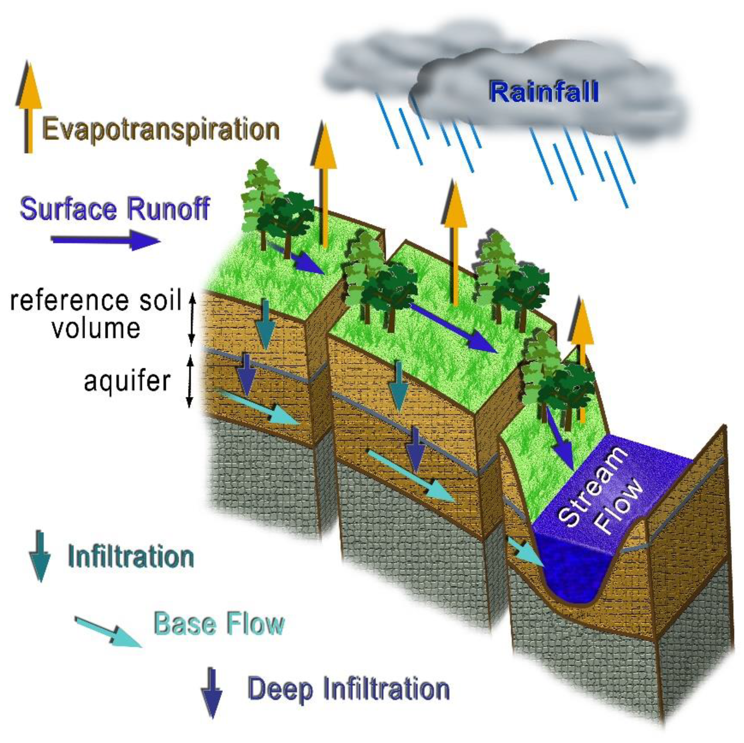
The design of the conceptual scheme of the model accomplishes the following targets: (i) makes use of well-established but simplified methods for the simulation of the involved hydrological processes, (ii) requires readily available or easy-to-obtain spatial data and parameters, (iii) adapts to Mediterranean conditions, (iv) efficiently describes vegetation-water dynamics, and (v) simulates crops irrigation.
Figure 1 presents the core of the conceptual scheme and the involved storages and flows.
The water content of the reference soil volume is directly involved in the calculation of most water balance components such as actual evapotranspiration, infiltration, direct runoff and deep infiltration, as well as in the estimation of crop water requirements. Thus, the following equation that describes the water balance of the reference soil volume (
Figure 1) has a central role in the hydrological model operation.
In this equation, RSWCi−1 and RSWCi (mm) are the reference soil volume water contents of the previous and the current day, respectively, and Pi (mm), Qi (mm), αETi (mm) and DΙi (mm) are the total precipitation depth, the direct runoff depth, the actual evapotranspiration depth and the deep infiltration depth of the current day, correspondingly. The reference soil volume is defined as the topsoil layer. In very deep soils, it is limited by the rooting depth.
In wet periods RSWC may increase up to a maximum value, which equals to the water holding capacity of the reference soil volume (RSWHC). Increased RSWC values result in reduced infiltration rates, increased actual evapotranspiration rates and increased deep infiltration rates. In contrast, in dry periods when soil becomes very dry, actual evapotranspiration, deep infiltration and effective rainfall are limited. The initial value of RSWC is the primary initial condition for the application of the model; however, its determination is challenging. For this reason, the model’s application requires a warm-up period, during which RSWC is adjusted by the success of very wet winter periods or very dry summer periods when RSWC equals to the RSWHC or zero, respectively.
2.1.2. Simulation of Hydrological Processes
Direct runoff is calculated using the Soil Conservation Service Curve Number (SCS-CN) method, which is very well documented and one of the most widely used conceptual methods for the estimation of runoff response [
44,
47,
48,
49,
50,
51,
52,
53,
54]. This simple but effective method directly accounts for most of the factors affecting runoff generation, such as land use/cover and soil by using only one parameter.
Specifically, the following equation calculates the direct runoff depth:
where
P is the total rainfall depth (mm) (in this case the daily rainfall depth),
λ is the initial abstraction ratio,
Q is the direct runoff depth (mm), and
S is the potential maximum retention depth (mm) expressed in terms of a dimensionless curve number (
CN) parameter as follows:
In this study, the initial abstraction ratio is set to the typical value (
λ = 0.2) in order for
CN to be the only unknown parameter of the method and to maintain the compatibility with the method documentation. In order to account for the effect of the soil’s antecedent moisture conditions (AMC) on runoff response, the estimated
CN values are adjusted according to the reference soil volume water content of each processed cell. Initially, the
CN values corresponding to dry (
CNI) and wet (
CNIII) conditions are estimated using the equations described in the method’s documentation based on
CN value for the typical conditions (
CNII) as described in the method’s documentation [
54]. Then, the
CN value is adjusted each day linearly between
CNI and
CNIII depending on the actual soil water content of the reference soil volume. More details on the SCS-CN method are present in [
44,
47,
48,
49,
50,
51,
52,
53,
54].
The estimation of the deep infiltration through the soil profile is through the Brooks and Corey [
55] equation assuming free drainage (zero pressure head) boundary condition at the bottom of the reference soil volume:
where
K represents the unsaturated soil hydraulic conductivity when soil moisture equals
θ,
Ks represents the saturated soil hydraulic conductivity,
θs is the soil moisture in saturation and
n is a shape factor. Base flow simulation uses the method of Arnold et al. [
56] and Hattermann et al. [
57]:
where
Qb,ι (mm) is the base flow in the day
i,
Qb,ι − 1 (mm) is the base flow in day
i − 1,
αb is the base flow reduction,
Wrch (mm) is the aquifer recharge in the day
i,
aq (mm) is the water quantity stored in the aquifer in the day
i, and
aqq (mm) is the limit of stored water, below which there is no base flow.
The calculation of the actual Evapotranspiration rate (
aET) draws on meteorological conditions, land cover and water availability in the reference soil volume. In this application, meteorological conditions are considered through the reference evapotranspiration (
ETo), which is a climatic variable computed from meteorological data. Reference evapotranspiration is calculated with the Food and Agriculture Organization (FAO) Penman–Monteith method [
58], which is a physically based method that closely approximates
ETo and explicitly incorporates both physiological and aerodynamic parameters. The meteorological data required are daily values of air temperature, solar radiation, air relative humidity and wind speed. Land cover characteristics (e.g., aerodynamic properties, albedo, stomatal characteristics, leaf anatomy) are considered through the crop coefficient (
Kc). In this way, potential evapotranspiration
ETp is calculated from
ETo as follows:
The
aET is finally calculated based on a water stress coefficient
Kst expressing the effect of water availability in the reference soil volume.
The values of Kc and Kst are determined for each grid cell and each day, depending on the vegetation characteristics of each place, based on the knowledge base, which contains information for a wide range of land cover types.
Irrigation water needs (
IRR) are calculated for the irrigated agricultural areas and for each time step as the difference between the evapotranspiration rate for standard optimal irrigated crop conditions that do not induce significant crop yield reduction and the actual evapotranspiration rate without irrigation of Equation (10).
The adjustment coefficient (
Sc) is the acceptable
ETp reduction rate without significant yield reduction [
58]. Typically, a value of
Sc equal to 0.90 is considered acceptable and was used in this application. However, the acceptable crop stress threshold can be adjusted for drought-tolerant crops or the simulation of deficit irrigation. Irrigation water application and distribution losses are considered on a later stage of the geospatial analysis as it is explained below. Finally, snow accumulation and snowmelt processes also are considered for higher altitudes through air temperature [
59].
2.1.3. Runoff Routing
Daily discharge for each grid cell of the stream network, for every time step, is estimated by adding the accumulated surface runoff for this time step to the accumulated base flow. Runoff routing through hillslopes (overland flow) and the stream network is carried out with a travel time approach [
45]. Travel times for the hillslopes (overland flow) and the channel network (channel flow) of the modelled area are calculated based on the flow velocity on each grid cell [
60]. To this end, the flow velocity grids for the overland flow and the channel flow are generated based on the land cover, the slope along the flow paths and the drainage network grids. The following equation computes flow velocity for overland flow (
Vo) as:
which is derived from the Manning equation assuming
. The coefficient
k is associated with land cover characteristics and the values corresponding to each land cover class estimated according to McCuen [
61]. The hydraulic gradient (
J) is considered equal to the slope along the flow paths (mm
−1). The flow velocity for channel flow (
Vc) is calculated using Manning’s equation:
where the roughness coefficient (
n) ranges from 0.055 to 0.025, according to the stream order of each segment [
62]. The hydraulic radius (
R) for each grid cell of the drainage network is determined by a power law relationship [
63], which relates hydraulic radius to the upstream area and provides a representation of the average behaviour of the channel geometry:
where (
Ad) is the drained area upstream of the cell in square kilometres, which is determined by the flow accumulation routine of the GIS, (
a) is a network constant and (
b) a geometry scaling exponent, both depending on the discharge frequency. The parameters
a and
b usually set equal to 0.07 and 0.43, respectively, to correspond to regular storm events [
62]. The hydraulic gradient (
J) is again considered equal to the slope along the flow paths (mm
−1).
The two flow velocity grids (for overland and channel flow) are overlayed, and the final flow velocity grid for each catchment is calculated. The final flow velocity grid is expressed in time per unit length units, which is the time necessary for the water to cross a distance of one meter, to facilitate the calculation of the travel time for each grid cell.
This methodology does not aim at producing very detailed hydrographs, but it is sufficient for water balance modelling at a daily time step.
2.1.4. Geospatial Analysis
The results of the model are aggregated for each year. They are stored to a specially designed geo-information system that includes all the data and the methods essential for the analysis of the results, the estimation of the impact indicator values and the estimation of the net effect of the RDP on the reduction of water abstraction in agriculture.
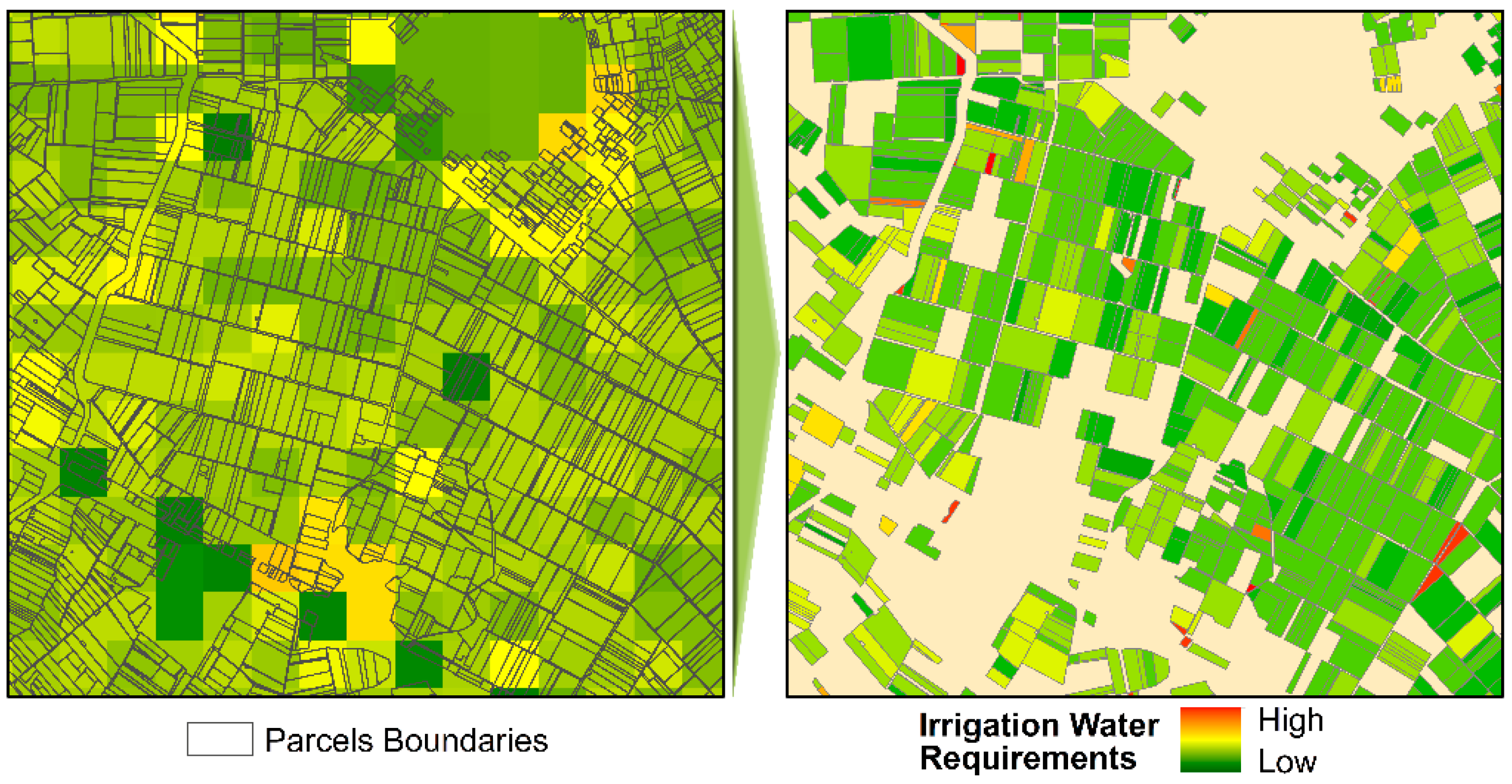
The significant problem is that even if the model can operate in very fine spatial resolutions, the resolution required for the accurate representation of the typically tiny farms would be prohibited in terms of computational requirements (
Figure 2). To overcome this problem, a larger cell size of 300 m sounds like a suitable compromise. Then, a unique algorithm was developed to link the polygon of each parcel in the IACS spatial database, with the nearest corresponding grid cell of the model having the same crop and the same conditions (e.g., soil, weather) (
Figure 2). In this way, the developed approach can provide information at the parcel level, and therefore facilitate the further analysis of the results and the estimation of water abstractions in agriculture by considering the precise boundaries of the irrigated parcels and all the relevant information included in the IACS database (e.g., crop, applied agri-environmental measures, irrigation system, water source).
Following the estimation of the irrigation water needs depth for each parcel and each year, the corresponding irrigation water volumes for each field are estimated considering the area of each parcel. Then, the distribution network losses and the irrigation water application losses are estimated. The distribution network losses are estimated based on the water source described in IACS database and the reported losses percentages (
Table 1). The corresponding irrigation water application losses were also estimated based on average losses percentages for the various irrigation systems categories described in the IACS database (
Table 1).
The total water abstractions for each parcel were finally calculated by summing all the abovedescribed factors. The obtained results were analysed, and various statistics were calculated for the studied years. Water abstractions also were aggregated at various administrative levels boundaries and for the different crop types.
2.2. Application
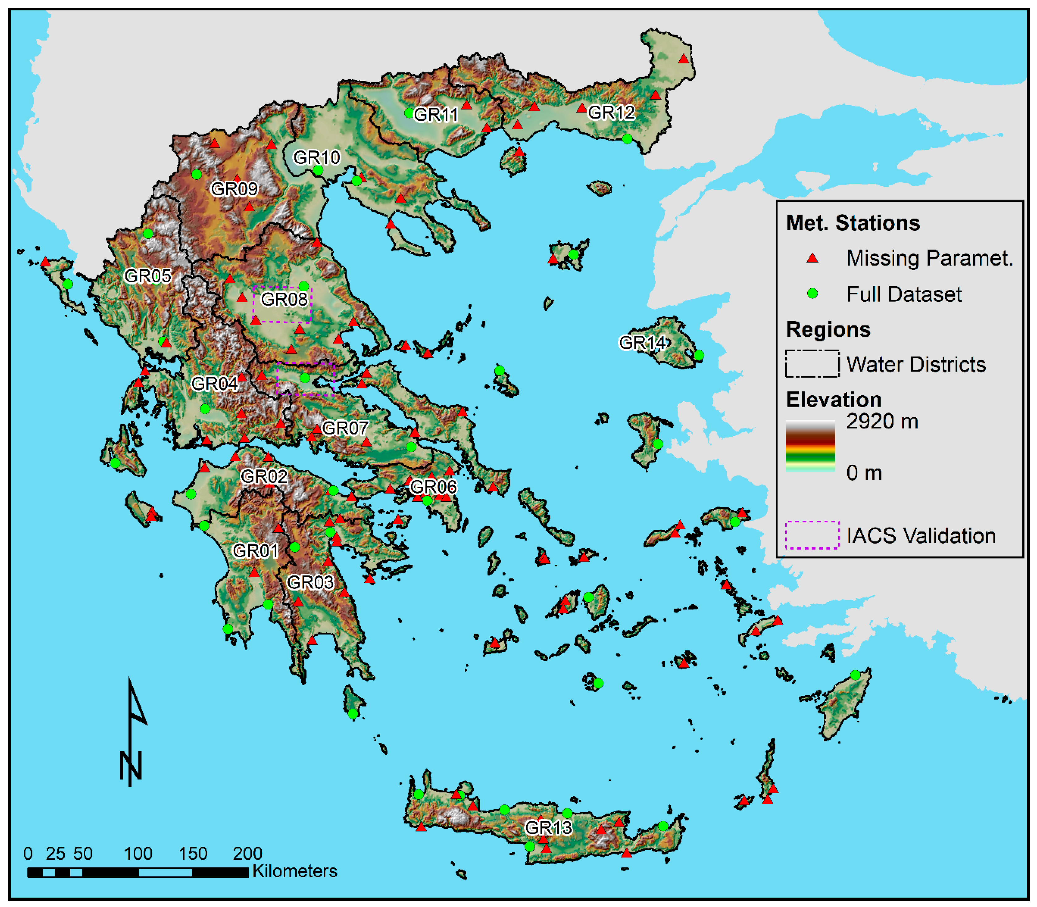
The model was applied for 34 years (1971–2004) all over Greece (country scale, area ≅ 131,940 km
2,
Figure 3), using a different setup for each modelled case. Specifically, it was applied using as input a land cover dataset consisting of the IACS database for the base year (2015) and the evaluated year (2018) in order to evaluate the effect of the implementation of RDP from 2015 to 2018 on water abstractions in agriculture. The model used the latest CORINE land cover (2018) for the nonagricultural areas that are not covered by the IACS database. In this way, the total water abstractions for each parcel were estimated for the crop patterns and cultivation practices existing in 2015 and 2018 for the reference meteorological conditions (1971–2004) and included as information in the IACS database for each year. The obtained results were analysed to estimate the values of the common impact indicators and answer to the common evaluation questions (CEQ).
Finally, it should be mentioned that the first year of the simulation period was used as a warm-up period in order to initialise the soil moisture spatial distribution, which is an initial condition that is not feasible to be directly estimated.
2.2.1. Input Data
The study used meteorological data from 140 meteorological stations of the Hellenic National Meteorological Service (HNMS) [
64] distributed over the whole country (
Figure 3) [
21]. The number of meteorological stations is adequate, considering the size of the study area. However, the vast spatial variability of meteorological conditions in Greece and the uneven density of stations across the country made necessary the use of specially adapted interpolation techniques as explained previously in the description of the methodology. Furthermore, most of the 140 meteorological stations’ data series had gaps or did not record all the required weather parameters (
Figure 3). Accordingly, the available datasets were assessed for integrity and consistency, and a gap-filling algorithm was applied as described in [
21]. The data used in this study consist of a daily data series for precipitation (
P) as well as for minimum, maximum, and average temperature, mean relative humidity, wind speed at 2 m height, and solar radiation or sunshine hours for the estimation of
ETo with the FAO Penman–Monteith method [
58].
The land use and land cover for the two studied years was based on the Integrated Administration and Control System (IACS) spatial database for the base year (2015) and the evaluated year (2018). IACS provides detailed spatial information at farm level (one polygon for each parcel) for all agricultural land each year and also contains detailed information on the cultivated crop in each parcel, the irrigation and the agri-environmental measures. The model used the CORINE land cover 2018 for the non-agricultural areas which are not covered by the IACS spatial database [
65].
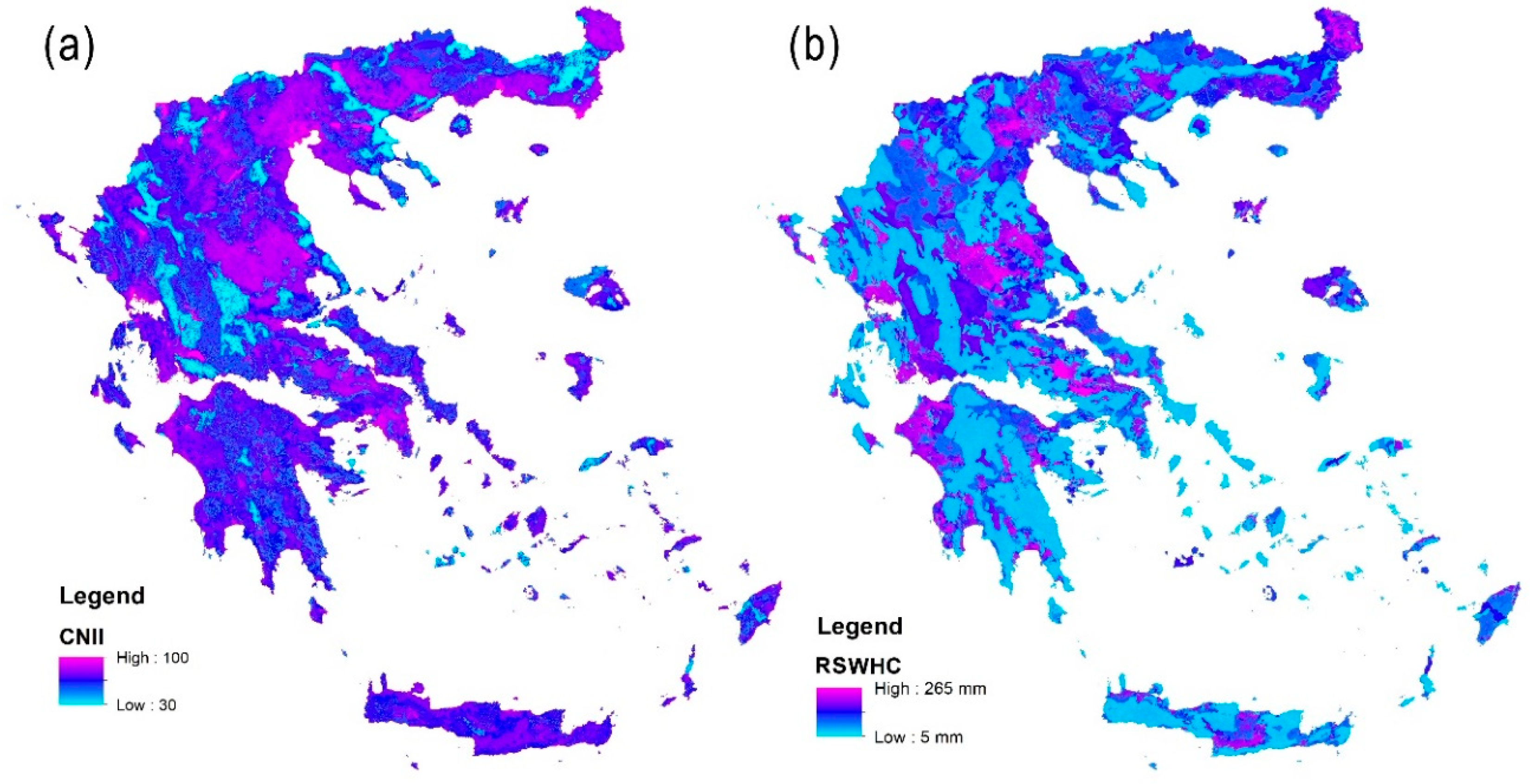
The study combined soil data from various sources in order to define the Hydrologic Soil Groups (HSG) required for the determination of
CN values and the required soil hydraulic properties (
Figure 4). The basic information was the soil map of Greece (scale 1:30,000) [
66], which covers most of the cultivated areas. For the remaining areas, the study made use of data sources like the European Soil Database (European Soil Database v2.0, scale 1:1,000,000) [
67] and the topsoil physical properties for Europe based on Land Use/Cover Area frame Survey (LUCAS) topsoil data [
67,
68].
The spatial distribution of the curve number for the typical conditions (
CNII) was determined based on the soil and the land use/cover (LULC) layers described above. To this end, the HSG spatial distribution was determined based on the soil data. The HSG layer was then combined with the LULC layer to determine the soil—land use/cover complexes for each grid cell of the study area. The determination of the
CN value for each grid cell (
Figure 4a) utilised an adapted lookup table based on the SCS-CN method’s documentation [
54] to comply with the IACS and the CORINE LULC classes.
Finally, the digital elevation model (DEM) used in this application came from the Shuttle Radar Topography Mission (SRTM) [
69]. The original spatial resolution of the DEM was 90 m × 90 m, resampled to 300 m × 300 m, which is the spatial resolution used in the model, like the rest of the data.
2.2.2. Remote Sensing
Although IACS data are considered very reliable, they can still contain errors, e.g., due to false claims or digitisation errors or some farmers might not apply for any subsidies [
70]. Therefore, the study used Sentinel-2 (S2) data for crop mapping and the validation of IACS’ declared parcels, for two characteristic water districts of Greece, namely GR08 (Thessaly) and GR07 (E. Sterea Ellas) (
Figure 3).
The Sentinels are satellites developed to support the Community’s Copernicus program. The S2 mission of the European Space Agency (ESA) provides imagery of very high spatial (10 m) and temporal (5 days cycle) resolution. Given its Multi-Spectral Imager (MSI) sensor, it operates on 13 different spectral bands covering the Visible (VIS, 4 bands: 1-2-3-4), Near Infrared (NIR, 5 bands: 5-6-7-8-8A, four of them are red edge bands) and Short-Wave Infrared (SWIR, 4 bands: 9-10-11-12) portions of the electromagnetic spectrum. Thus, it can deliver innovative and continuous data, and it is a unique tool for monitoring crop conditions, seasonal changes and crop classification, etc. [
71].
To distinguish the existing crop types for the evaluation of the declared parcels dataset, the study acquired (via the ESA Open Access Hub,
https://scihub.copernicus.eu, accessed on 29 March 2020) four freely available, cloud-free S2 images, geometrically and atmospherically corrected (Bottom-Of-Atmosphere, 2A processing level), representative of the 2018 agronomic season.
The data pre-processing involved image resampling (10 m, since S2 images have different pixel sizes), subset and masking (excluding pixels outside those selected). Finally, the stack (collocation) of 10 spectral bands for each date was executed by excluding bands 1 (coastal aerosol), 9 (water vapour) and 10 (cirrus). Subsequently, mapping the target classes relied on supervised classifications using the Random Forest (RF) classifier, a non-parametric decision tree machine learning algorithm. Contrary to parametric classifiers, RF examines the association between the training and the response dataset. It is a predictive model that recursively splits a dataset into regions by using a set of binary rules to compute a target value for classification purposes. Multiple decision trees (forming an RF) are created during training, after which the mode of the provided classes of the individual trees sets the output class of the forest [
71,
72,
73,
74]. RF requires the adjustment of two parameters, the number of trees which will be created by randomly selecting records from the training samples and the number of variables used for tree nodes. In the present research, RF run used the RF classification toolbox of the Sentinel Application Platform (SNAP) provided by the European Space Agency (
http://step.esa.int/main/toolboxes/snap, accessed on 9 January 2020).
The classification training samples included 140 and 120 points for the two regions, respectively. The reference samples were split into two sets of separate training (70%) and validation reference samples (30%). A two-step classification procedure used the first training set, and 6 classes (summer-fodder crops, winter crops, set aside-bare soils, orchards-olives, artificial surfaces and water). The first step comprised a broad distinction among crops and forest, water and built-up classes. The second step further classified the crops.
2.2.3. Calibration Validation
As regards to the hydrological balance, the model has been already successfully calibrated and validated in previous studies [
5,
36]. Also, it has been tested for specific parts of the studied region [
39,
40]. The model was also tested based on the current configuration and input data providing similar performance with the previous applications [
5,
36]. It should be noted though that, due to the acute scarcity of reliable hydrological data and the vast study region as compared to the time and financial constraints of the current study, a thorough calibration and validation of the applied hydrological model was not feasible at this stage. Considering also that the most critical information for this application is the water abstractions in agriculture, model testing focused on the estimation of irrigation water needs. The key parameters that may influence the irrigation water needs are the soil hydraulic properties, the crop-related coefficients (
Kc,
Kst,
Sc) and the losses percentages. To check if the selection of percentage losses and crop coefficients is appropriate, the model’s result was tested on specific case studies (e.g., using data from local water distribution authorities for collective irrigation networks water abstractions, and estimations from case study farms). Generally, the obtained results were comparable with the estimations mentioned above except for some specific crops like olive groves or vineyards, where a systematic overestimation was observed, possibly because deficit irrigation is the norm in these crops. Thus, future work should focus on the detailed calibration of the
Sc parameter specifically for each crop. Furthermore, a more detailed calibration/estimation of losses should be made in pilot case studies with diverse characteristics and with various water sources, distribution networks and irrigation systems. Also, it should be noted that the same approach and parameters were used in both examined scenarios; therefore, the expectation is that the estimation of changes will be more accurate because of the elimination of possible systematic errors.
It should be underlined that the available water abstraction data are minimal. When they exist, their documentation and metadata are weak, and they mostly concern the recent few years, and so it is hard to make critical, safe comparisons. Accordingly, the next step is the more exhausting calibration, and validation of the model as more detailed data are becoming available.
2.3. Counterfactual Analysis
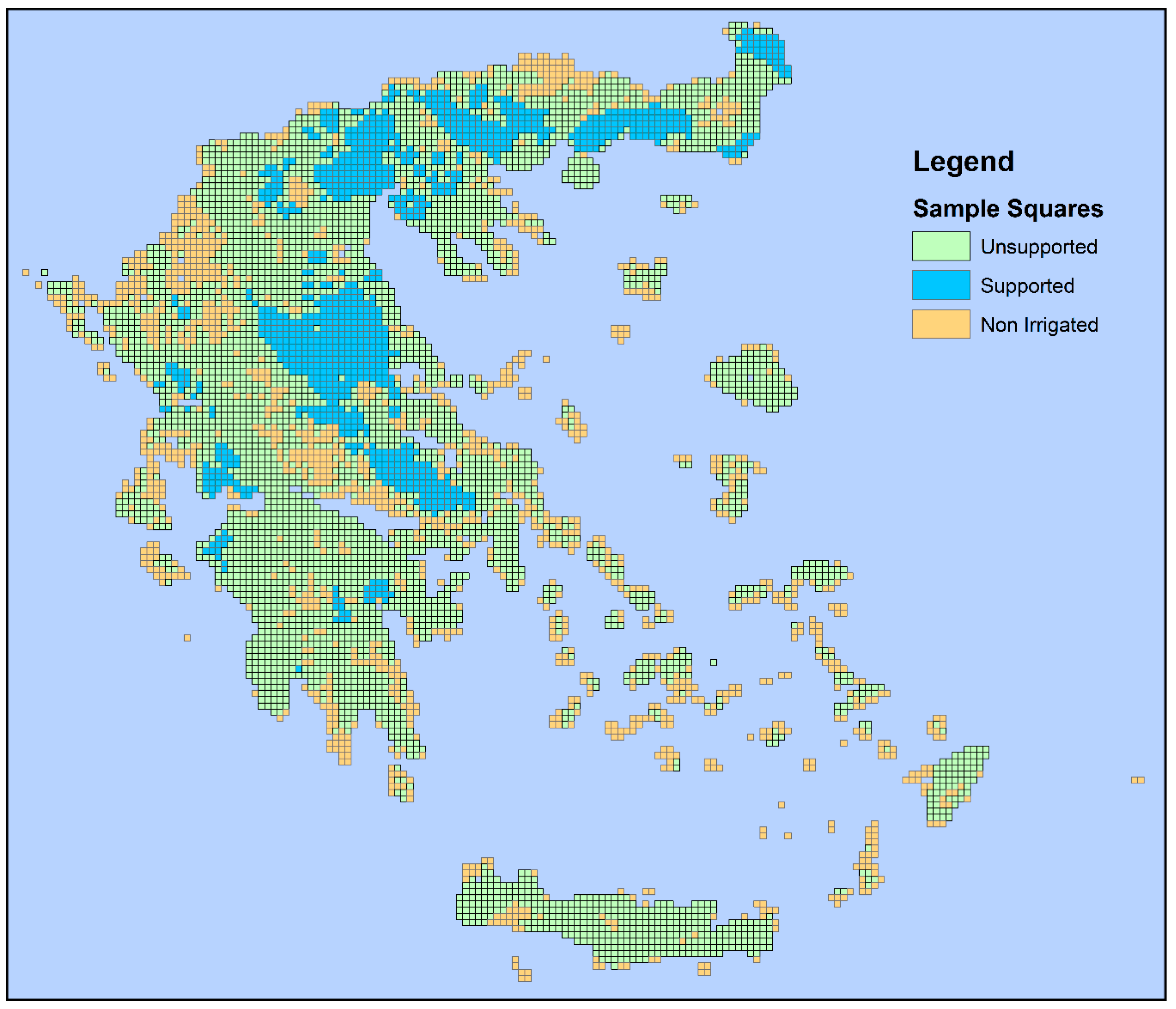
The evaluation aims at determining the policy’s net effects on irrigation water savings. In essence, evaluation establishes the real impacts of a CAP measure. There are many factors, beyond the operation of AEMs, which can have an impact on agricultural land use patterns and, consequently, on water savings. For example, taking into account the high cost of irrigation, a cost-minimising farmer may choose a mix of cultivations that minimises energy for irrigation costs under expected yields and prices. This decision will, inevitably, produce considerable water savings without the influence of a policy measure. Thus, evaluation attempts to isolate the influence of a policy’s measure on the values of water savings from the influence of other contextual factors or interventions. What would have happened to beneficiaries in the absence of the AEMs is called the “counterfactual”. The net effect of the measure compares the counterfactual outcomes, i.e., outcomes without AEMs, to those observed under the AEMs. Evaluators compare a sample of units that are under the influence of the measure (policy on) with a corresponding sample of units which is not influenced by the measure (policy off). In evaluation terminology, the former is the “treatment” group or the group of “policy beneficiaries”, and the latter is the “control” group or the group of “policy non-beneficiaries”.
In similar evaluations, the farm is the primary statistical unit, because this is the level at which farmers consider their alternatives and make their optimisation decisions. However, the IACS database provides information only at the farm parcel level, and it does not link the parcels of land farmed by the same decision-maker. The evaluators overcome this significant data limitation by creating a canvas of 5 × 5 km (25 km
2) squares which cover the entire national territory. In this perspective, each square is a large farm whose land-use allocation is the outcome of the simultaneous decisions made by farmers cultivating parcels within the square boundaries. For each square, the hydrological model provides estimates of the needs for crop irrigation water. Besides, for each square, the evaluators know the area under AEMs and a range of physical and agronomic characteristics. The latter include the square’s average height, its mean slope, prevailing soil conditions, average rainfall, mean evaporation, and others. In total, 6418 squares cover the whole territory, of which 4897 contain plots with irrigated land and form the population of the evaluation study. From the population of 4897 squares, a stratum of 1044 squares contains parcels operating under the AEMs, i.e., squares that contain “beneficiaries”. From this stratum, the evaluation can draw the “treatment” sample of squares. The rest of the 3853 squares do not contain any parcels operating under the AEMs and thus are squares of “non-beneficiaries”. From this stratum of “non-beneficiaries”, the evaluation can draw the “control” sample of squares.
Figure 5 shows the distribution of the sample squares.
One of the methods available to avoid biased comparisons between “control” and “treatment” squares is to match each “treatment” square with a similar, if not identical, “control” square. Matching pairs ensures that the evaluation compares pairs of almost identical subjects that differ only by the operation of the measure. After a successful matching, the mean values of a range of matching variables between “control” and “treatment” groups are not statistically different. Among the available matching pairs algorithms, this evaluation uses the propensity score matching.
3. Results
The model was applied for 34 years (1971–2004) using a different setup for each modelled case, and it allowed the estimation of the different components of water balance all over Greece as well as vegetation water deficit and crop water needs. Specifically, the model was applied using as input the IACS database for the base year (2015) and the evaluated year (2018), correspondingly. In this way, the total water abstractions for each parcel were estimated for the crop patterns and cultivation practices existing in 2015 and 2018 for the reference meteorological conditions (1971–2004) and included as information in the IACS database for each case.
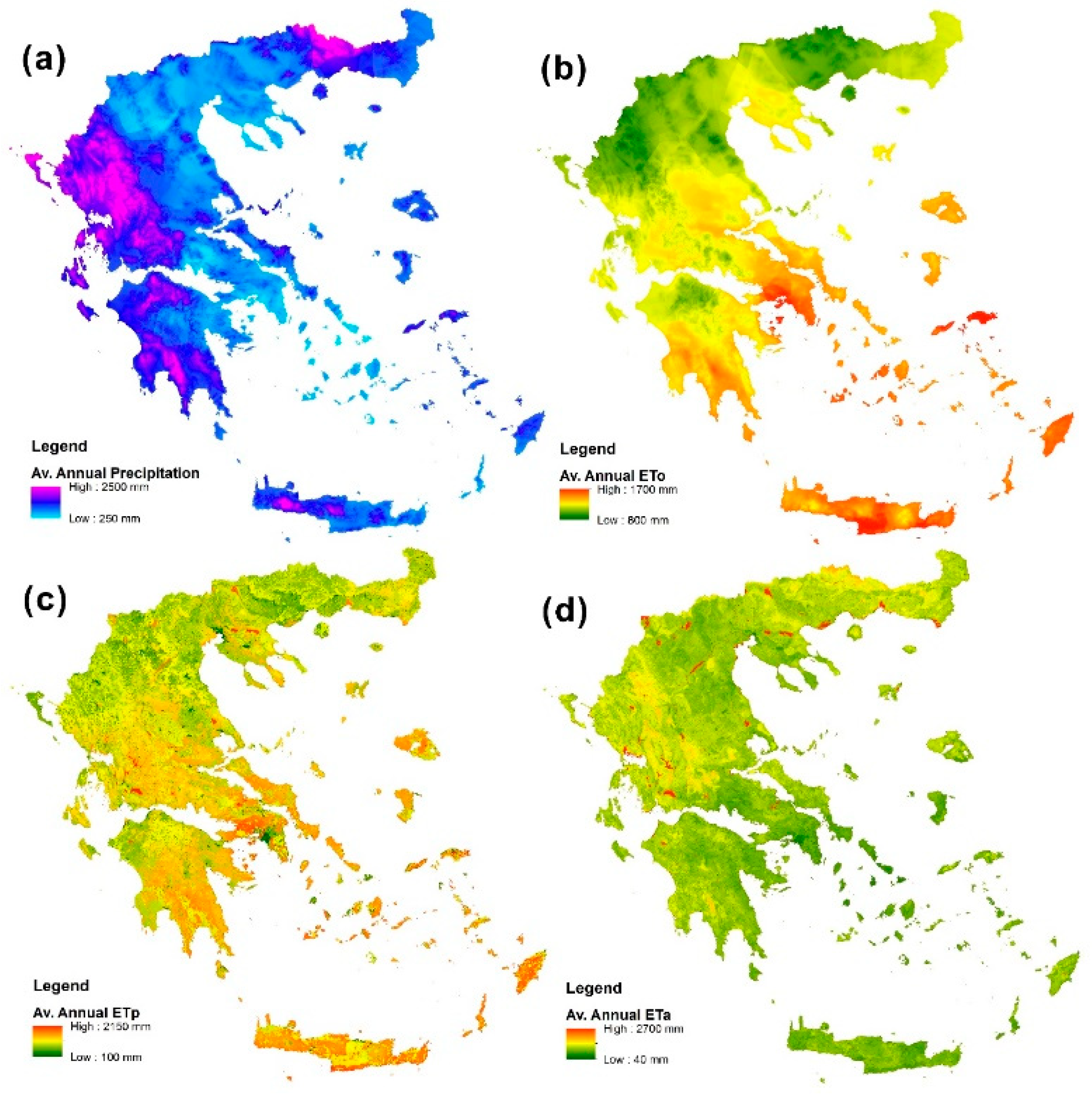
In
Figure 6a, the average annual precipitation depth spatially distribution for the study period is illustrated. The extensive spatial variability of the annual precipitation depth ranges from well above 2000 mm/year at the northwest mountainous areas to below 300 mm/year at the eastern part of the country and especially in the central Aegean islands. The extensive spatial variability in comparison to the relatively small size of the country may be due to the massive sierra with a north–south direction that divides the mainland of the country and to the very long coastline [
21,
36]. The spatial distributions of average annual reference, potential and actual evapotranspiration depths are presented in
Figure 6b–d, correspondingly. It is evident that
ETo spatial distribution is not correlated with the spatial distribution of precipitation and many areas with low precipitation have at the same time high
ETo. Potential evapotranspiration is more diverse, as also it is influenced by land cover properties (
Figure 6c). Interestingly, areas with high
ETo and
ETp values are characterised by low actual evapotranspiration depths (
Figure 6d). In dryer areas,
ETa is controlled by soil water availability, which is limited by lower precipitation depths and smaller soil water holding capacities.
The high temporal variability of precipitation (not shown here) is an additional important factor affecting water availability as most of the water abstractions take place in the dry season (May to September) [
36].
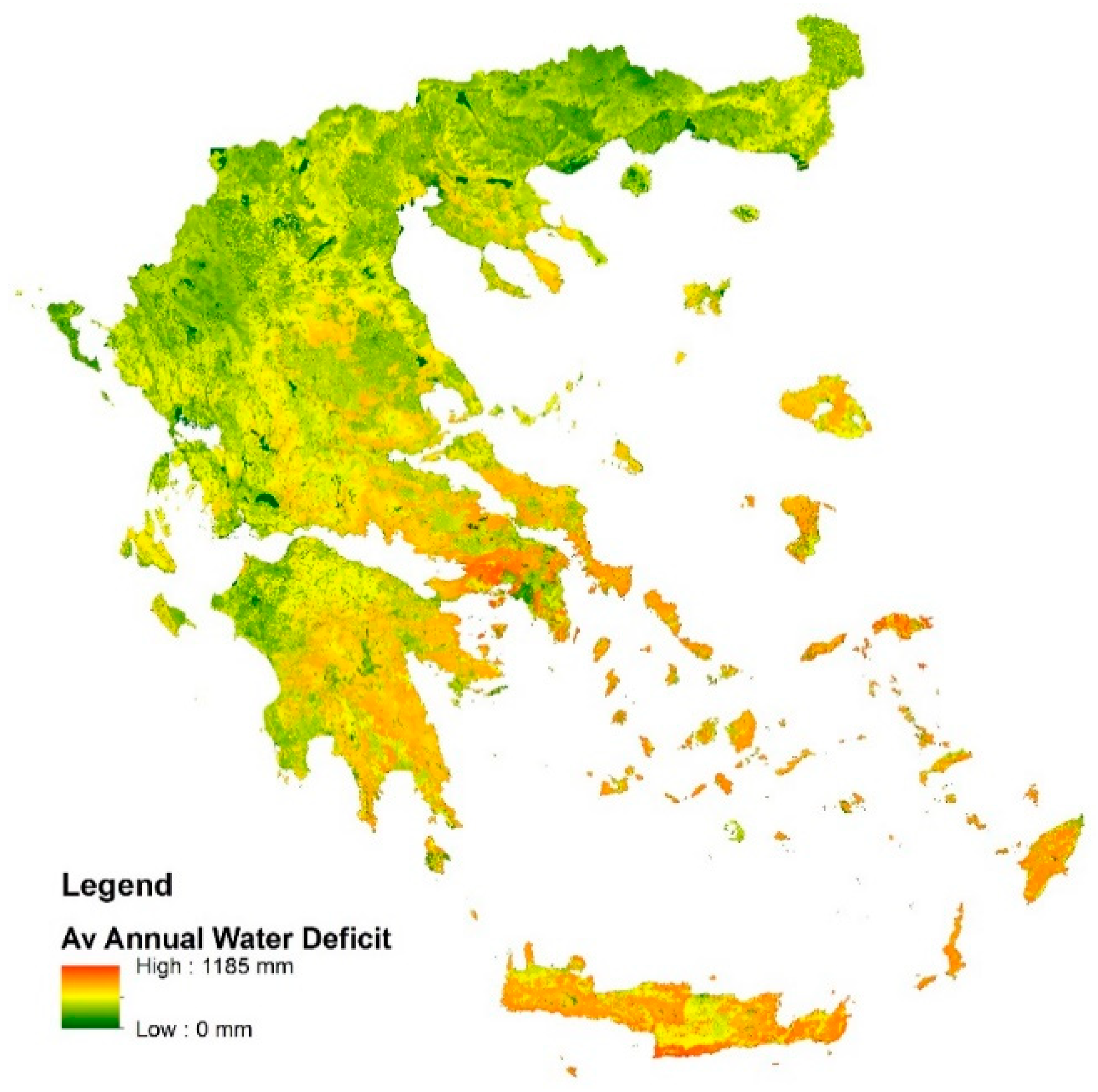
The spatial distribution of the average annual vegetation water deficit (
Figure 7) is related more to
ETp than to precipitation. The most significant part of water deficits is observed during the dry season, when precipitation is meagre in all areas; thus, in areas with higher
ETp, higher deficits are observed. Increased water deficits indicate areas with higher desertification risk [
75,
76,
77]. The same figure shows that irrigation water needs are higher in southern Greece and mostly in the southeast part of the country.
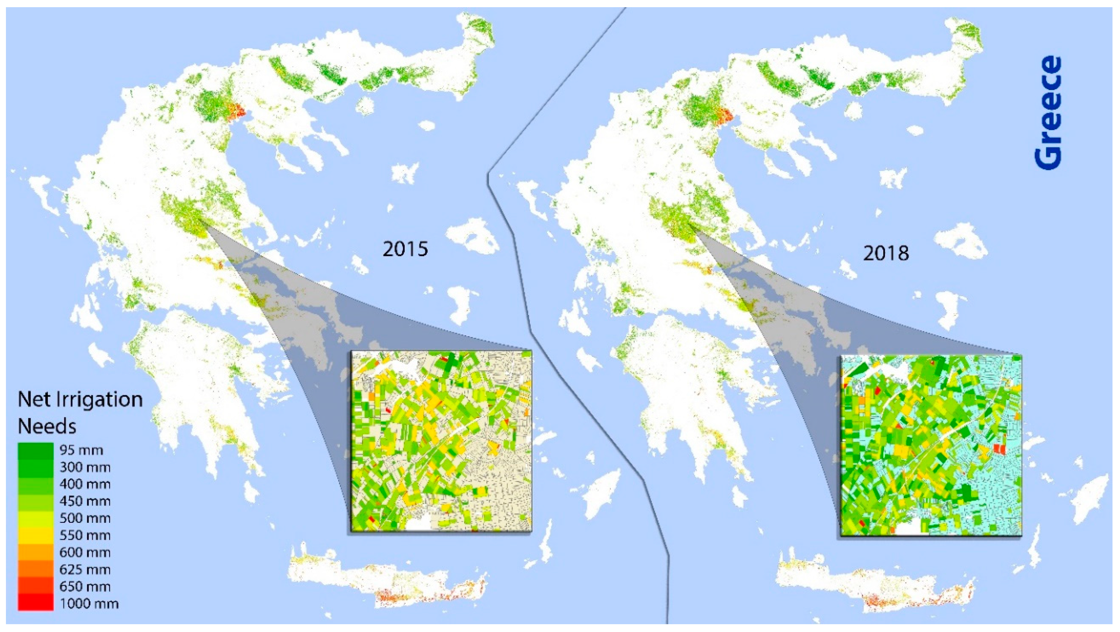
The above results were linked with the parcel polygons of the IACS spatial database (about 6,000,000 polygons) and integrated into the database mentioned above. In this way, it was made possible to estimate more precisely the total water abstractions for each parcel and to investigate the effect of the agri-environmental measures on agricultural water use as these measures applied on each farm. As an example,
Figure 8 shows the net irrigation needs for each irrigated parcel for the 2015 and 2018 scenarios.
The obtained results were then analysed to estimate the values of the common impact indicators and answer to the common evaluation questions.
Table 2 presents summary results of irrigation water requirements and the corresponding total water abstractions in agriculture for the scenarios corresponding to the years 2015 and 2018. The total water abstractions for irrigation are higher in 2018 due to the increase in the irrigated area. In contrast, the water abstractions per cultivated area hectare are slightly lower in 2018.
The estimated total water abstractions for irrigation were also aggregated to the boundaries of the water districts of Greece to allow the comparison with the information included in the corresponding Master Plans on Water Resources Management [
78] for each water district and with other data sources and previous studies. As can be seen in
Table 3, the estimated total water abstractions are generally lower than the estimations included in the master plans for both scenarios. However, the difference is not considerable. Also, it is interesting to highlight that the total water abstractions calculated for the two scenarios are between the corresponding figures estimated by Soulis and Tsesmelis [
5] based on land cover data coming from CORINE Land Cover (CLC) 2000 and 2012 and statistics for the irrigated areas coming from ELSTAT (Hellenic Statistical Authority). It should be noted though that there are some more profound differences when specific water districts are considered. There is a general agreement though in the estimated abstractions for the larger plains of the eastern part of the country (e.g., Thessaly and Central Macedonia). Also, it can be seen that the irrigation needs in western Greece are considerably lower as the climate there is much wetter. On the other hand, it is worth noting that all estimations of total water abstractions in agriculture are considerably lower than the corresponding estimations presented in Eurostat for the annual water abstractions by source and sector [
79]. Specifically, for the years 2011 to 2015, the total water abstractions in agriculture reported in Eurostat are 8282.54 hm
3, while with the current methodology were equal to 6387.98 hm
3 for 2015 and 6634.03 hm
3 for 2018.
Table 4 presents a summary of the total irrigation water abstractions for the main irrigated crops. Cotton is the leading irrigation water consumer in Greece, followed by fodder crops and olive groves. As regards olive groves, however, results may be significantly overestimated. Specifically, the reported net irrigation needs depth (
Table 4) seems to be very high in comparisons with the water amounts used in typical farms. The high net irrigation needs depth can be attributed to the fact that olives are typically cultivated in the drier parts of the country. On the other hand, deficit irrigation or application of specific amounts of water at predefined development stages is the usual irrigation strategy in olive groves [
80,
81,
82,
83,
84,
85]. Still, it is an important observation that, even with deficit irrigation olive groves, that typically do not attract any attention when it comes to water consumption, they consume a large amount of water due to the extensive irrigated area (180,090 ha in 2018). The irrigated area is the third largest following cotton and fodder crops with a small difference. It should also be noted that this irrigation water is mostly consumed in the drier part of the country.
In order to investigate the quantification of the impact of RDP measures in the improvement of water use efficiency in agriculture, at first, the following approach applied. Initially, the measures that potentially have a direct or indirect impact in the water use efficiency in agriculture were identified. To analyse the changes in water use over time and under the RDP’s influence, the study identified the parcels that were supported by these measures in 2018 but were not supported in 2015. It was observed that these parcels had slightly higher total water abstractions (≅10 hm3) due to the larger irrigated area. However, they have slightly lower average irrigation needs depths (≅12 mm) and lower total water abstractions per hectare (≅152 m3/ha) or 2.7%. As regards the comparison of the cultivation patterns, there is a reduction in the areas cultivated with cotton and an increase in the areas cultivated with beans.
A more elaborate counterfactual analysis described in the methodology section shows that the net effects are considerable. The Average Treatment Effect (ATE) is the difference in average per hectare irrigation requirements between 1042 matched “treatment” and “control” squares (
Table 5). In treatment squares, irrigated land uses 852.46 m
3/ha less water. If we upscale this ATE estimate to the 142,331 ha under the AEM 10.1.4, we derive total net water savings of 121.3 million m
3. The net irrigation needs for 2018 are 4866.74 million m
3 (
Table 2). Thus, the net effect of 121.3 million m
3 corresponds to net proportional water savings of 2.5%.
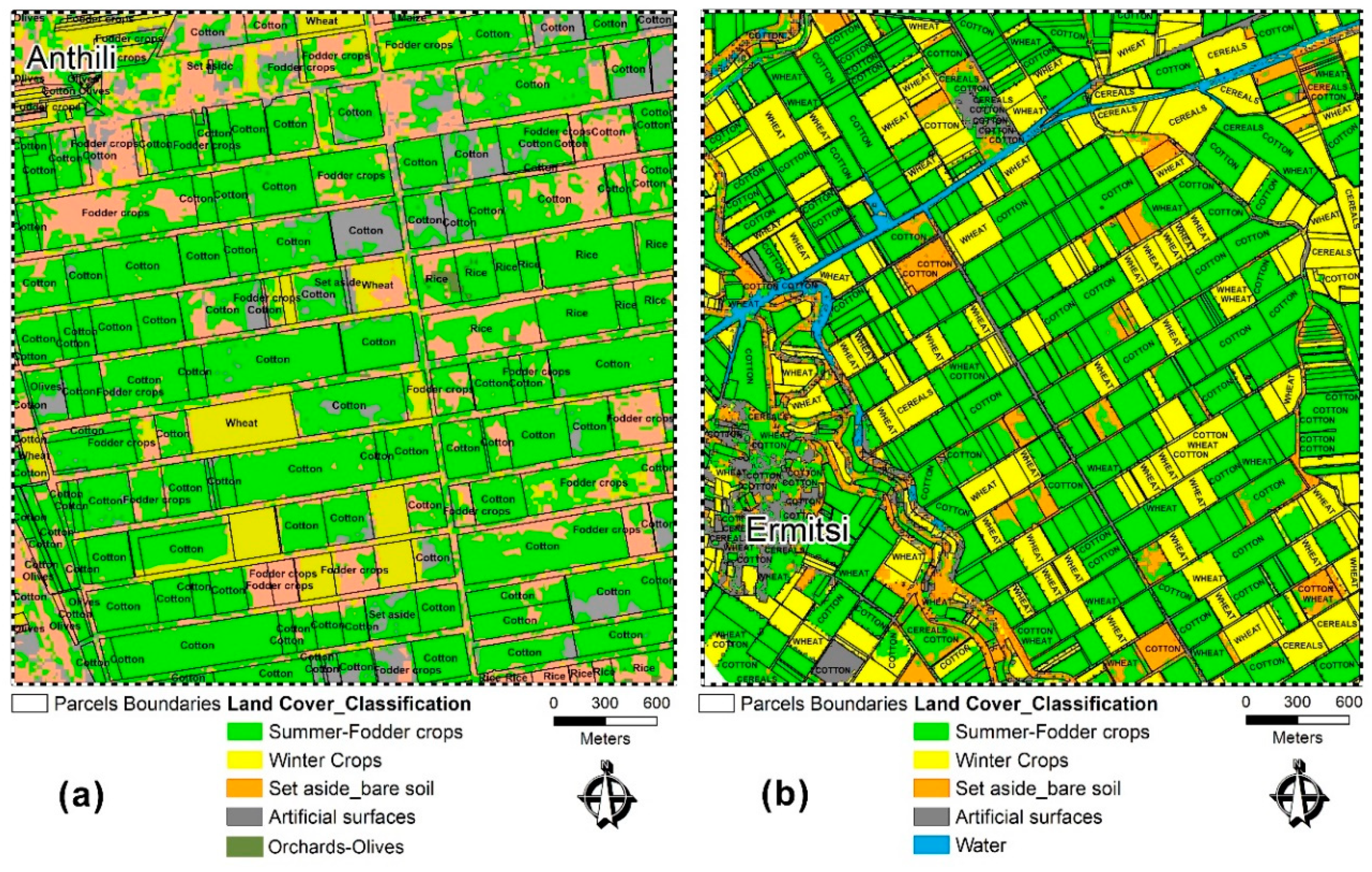
Finally, as regards the accuracy of the farmers’ declared crops database, the classification images of the two selected regions (Thessaly and Sterea Hellas) were used for its validation (
Figure 9). The accuracy assessment was accomplished using the second validation set. The results were evaluated using overall accuracy (OA), producer’s accuracy, user’s accuracy metrics [
86], and the Kappa coefficient [
87]. The classification OA and Kappa coefficient, for the Thessaly and Sterea Hellas regions, were estimated at 89.4% and 90.2%, and 0.71 and 0.74, respectively. The results indicate high accuracy in the farmland declaration process.
4. Discussion and Conclusions
Environmental objectives have recently become an integral part of CAP [
16,
17], which represents the critical form of public intervention influencing natural resources and environmental management [
18,
19]. The primary policy tool in CAPs environmental objectives are the agri-environment measures (AEMs) [
18]. Accordingly, efficient monitoring and evaluation of the impact of the agri-environment measures supported by the RDP on water resources are crucial for efficient policy design and adaptation.
According to the guidelines [
27], the most appropriate source so far is the Eurostat—Survey on Agricultural Production Methods. However, the data included in Eurostat for the annual water abstractions by source and sector [
79] are of questionable accuracy, and the corresponding data sources behind these data are unclear. Specifically, for the years 2011 to 2015, the total water abstractions in agriculture reported in Eurostat are 8282.54 hm
3, which are considerably higher from the estimations of the current study (6387.98 hm
3 for 2015 and 6634.03 hm
3 for 2018) as well as from the estimations included in the Master Plans on Water Resources Management [
78] (6875.7 hm
3) or from other previous studies [
5] (6447.7 hm
3). There is also a significant delay in the available data in the Eurostat database regarding agri-environmental indicators, and data collection level is, in most cases, only national.
Previous studies indicated that policy-driven monitoring and evaluation usually does not match the ideals of what is needed to inform adaptive management and that there is a tendency to focus on understanding state and trends rather than tracking the effect of interventions [
88].
For the present study, a specially developed model-based approach using multisource data, which is directly relevant to the evaluation of agricultural water policies, was applied to overcome the problems of small-sized and fragmented farms, vast spatial and temporal variability, and severe data scarcity. The study also developed an algorithm that links each parcel in the spatial database of IACS (over 6,000,000 polygons) with the nearest corresponding grid cell of the simulation model with the same crop and the same conditions. In this way, the proposed approach can provide detailed information at parcel level and facilitates the precise estimation of water abstractions in agriculture utilising all the pertinent information included in the IACS database (e.g., applied agri-environmental measures, irrigation system, water source). Hydrological modelling has also been proven to be a useful tool for the estimation of irrigation water needs in previous studies [
5,
32,
41].
The obtained results indicated that even if specific water abstractions per hectare of irrigated land were lower in 2018 after the implementation of the supported agri-environmental measures, the total water abstractions were higher. This result was due to the increase in the irrigated area. This fact should be taken into account in the design of future policies targeting a reduction in the footprint of agriculture on water resources. An important observation is also that total water abstractions for irrigation were much higher at the eastern and more dry part of the country, which should also be considered in future management plans. In general, the results of this study highlight the significant problem caused by the high spatial and temporal variability of available water resources and water requirements. As an example, even in the water district with the biggest total water abstractions for irrigation (Thessaly), these abstractions represent about 50% of the theoretical annual available water resources [
78]. Previous studies highlighted that optimising cropping patterns of the existing crops can result in an improvement of irrigation settings and in significant water savings [
9].
The applied methodology is efficient and fast, and it provides considerable flexibility that allows the investigation of several crop distribution patterns and climate scenarios. It produced valuable information concerning agricultural water use. It may additionally act as a useful assessment tool for the evaluation of land use or climate change impacts, and the assessment of adaptation and mitigation strategies. The provision of detailed information at the parcel level for the entire country makes it a powerful tool for policy design and evaluation.
Precise information on cultivated and irrigated area as well as on crop patterns is a crucial requirement for any detailed irrigation water abstractions assessment. IACS was proven to be a valuable database on this matter. It provides detailed information on the exact boundaries of all cultivated parcels in the country (more than 6,000,000 parcels) and detailed information on the cultivated crop, the applied agri-environmental measures and other relevant information. The results of the validation of the farmers’ declared crops database also indicate a high accuracy in the farmland declaration process. However, the current study also highlighted some remaining significant problems in the IACS spatial database that hinder its broader utilisation. The main problems are:
The IACS spatial database in Greece provides information only at the parcel level without any information on how parcels link to farms. Typically, the farm is the decision-making unit because farmers optimise the farm’s resource use by taking into account constraints on a parcel basis. This lack of information caused additional difficulty.
Different polygons and codes for the parcels are used by the IACS database each year. Therefore, direct interannual comparisons are not feasible.
Some agricultural areas are not included in the IACS database, and thus, the area included in the IACS differs each year.
There is a lack of metadata/documentation for the IACS spatial database. For this reason, it was difficult to interpret some of the cultivation codes, the meaning of more than one cultivation codes for one parcel, or some additional information on irrigation.
Even though, the main alternative, which is CORINE land cover, does not provide sufficient resolution and accuracy on agricultural areas. Additionally, a very high percentage of the area is characterised by complex patterns (e.g., crops/natural vegetation).
The more prominent use of secondary data and more transparency in data-sharing are essential in enabling adaptive management to safeguard socioecological systems [
88].
A limitation of the current study is due to the lack of available water abstractions data with adequate documentation and metadata that would allow a more detailed calibration and validation of the model. Future research should focus on exhaustive calibration and validation to specific pilot sites as more detailed data are becoming available. These detailed data are crucial, especially for crops like olive groves or vineyards, where deficit irrigation is the norm as well as for the estimation of “conveyance” and on-farm losses.


