Spatiotemporal Change Analysis and Future Scenario of LULC Using the CA-ANN Approach: A Case Study of the Greater Bay Area, China

Abstract

Land use land cover (LULC) transition analysis is a systematic approach that helps in understanding physical and human involvement in the natural environment and sustainable development. The study of the spatiotemporal shifting pattern of LULC, the simulation of future scenarios and the intensity analysis at the interval, category and transition levels provide a comprehensive prospect to determine current and future development scenarios. In this study, we used multitemporal remote sensing data from 1980–2020 with a 10-year interval, explanatory variables (Digital Elevation Model (DEM), slope, population, GDP, distance from roads, distance from the city center and distance from streams) and an integrated CA-ANN approach within the MOLUSCE plugin of QGIS to model the spatiotemporal change transition potential and future LULC simulation in the Greater Bay Area. The results indicate that physical and socioeconomic driving factors have significant impacts on the landscape patterns. Over the last four decades, the study area experienced rapid urban expansion (4.75% to 14.75%), resulting in the loss of forest (53.49% to 50.57%), cropland (21.85% to 16.04%) and grassland (13.89% to 12.05%). The projected results (2030–2050) also endorse the increasing trend in built-up area, forest, and water at the cost of substantial amounts of cropland and grassland.

1. Introduction

Landscape change is based on the natural ecosystem and the structure of human society. The process of landscape change results from changes in the physical environment and socioeconomic factors [1]. Fast economic development and population growth results in rapid urbanization and land-use changes. These changes significantly affect LULC dynamics and the cycle and structure of the ecosystem [2]. Anthropogenic influence on landscapes is one of the fundamental driving forces of regional LULC change mechanisms [3,4]. Human exploitation of the natural environment, such as urban expansion, fragmentation of agricultural land and green spaces, expressively disturbs the local environment [5]. Among these activities, rapid urban growth is considered the leading driver of cropland and green area losses [6], which may greatly influence climatic changes and human life [7,8]. The dynamics of socioeconomic development and industrialization have led to a drastic expansion of built-up areas in periurban regions. Such an increase in impervious surfaces affects the urban environment [9].

Global LULC trends are divided into two categories: intensification, such as deforestation, agricultural and urban expansion; and extensification, such as afforestation and land protection. Intensification refers to the rapid urban and agricultural expansion in the natural landscape, whereas extensification is the proposed strategies to control the rapid LULC transition and its impacts on natural environment [10,11]. Globally, the level of urbanization is estimated to be approximately 55% [12]. More than half of the global population lives in urban areas, and this value will reach approximately 70% by 2050 [13]. However, urbanization is increasing at double the pace of global population growth [14,15]. The urbanization process in developed countries is more synchronized, and most of these countries stabilize the urbanization level [16]. Developing countries are experiencing over or under-urbanization [17]. Urbanization and socioeconomic development are closely correlated, as socioeconomic development stimulates urbanization [18]. Nearly 80% of the global GDP is generated in cities [19], and activities related to economic growth persuade migration, which is one of the major driving forces of urbanization [20]. Additionally, urban poverty is increasing globally, which is mainly attributed to rapid migration (www.unfpa.org/urbanization, accessed on 10 August 2020). Consequently, unprecedented urban expansion and population growth trigger LULC changes, which can potentially cause ecological consequences such as substantial soil erosion, carbon emissions, climate change and groundwater resource degradation [21,22,23]. Furthermore, tremendous urban expansion and socioeconomic development have placed enormous pressure on natural resources, ecosystems [24] and the fragmentation of agricultural land, becoming significant reasons for environmental disruptions, food security issues and impacts on human health around the globe [25]

The urbanization rate in China increased from 17.9% in 1978 to 56.7% in 2016 [26], and the urban population increased by 500 million from 1980 to 2011 [27]. It is expected that the urbanization rate will reach 70% by 2050 [28], and is projected to add 255 million urban dwellers by 2050 [18]. Over the last four decades, China’s cropland area has experienced uneven changes [29], especially in the Pearl River Delta, due to rapid urban expansion [30]. Although the rapid increase in built-up land promoted the local economy, it also brought severe concerns to meet sustainable development targets [31]. Therefore, the LULC change mechanism becomes an essential aspect for studying and understanding the complicated relationship between humans and the natural environment.

Since its economic reforms, China has been experiencing rapid urban expansion resulting in the loss of substantial agricultural land [32] and green spaces. The Chinese government introduced a series of land administration policies to minimize the fragmentation of cultivated land and green space, but as urbanization is the driving force for economic growth [33], it is a challenge to enforce the policy by compromising economic growth [27]. Additionally, urbanization influences atmospheric pressure, evaporation, the absorption of heat, and solar radiation, and can significantly change the surface temperature conditions [34]. Hence, anthropogenic modifications tend to experience comparatively higher environmental degradation than the surrounding LULC categories [35]. All these issues make LULC change analysis a paramount concern of sustainable development. It plays a vital role in addressing and studying natural resources, the environment, and urban planning [36,37]. Several studies have shown that LULC changes, especially urban expansion, forest and biodiversity loss, fragmentation of agricultural land, water quality depletion, increased carbon emissions and temperature, are substantially related to the degradation of the natural environment [38,39,40,41,42]. Therefore, monitoring and detecting LULC change dynamics from the past to the future [43], especially under the influence of anthropogenic and physical factors and their contributions to local landscape changes, are critical for maintaining and integrating the ecosystem and sustainable development.

Spatiotemporal modeling, simulation and change transition potential techniques have evolved rapidly to study the LULC mechanism [44]. Simulation models of LULC transition and prediction are effective and replicable techniques for evaluating both the causes and the significance of past, present and future scenarios under possible situations [45,46]. Many spatially explicit models have been proposed by researchers to analyze and project the LULC, such as Dinamica [47], FLUS [45], SLEUTH [48], Artificial Neural Network-Markov Chain [49], CA-ANN [50], CLUE-S [51] and SERGoM [52]. Every model has its own specialty for addressing the composite issues of LULC. Among these models, cellular automata are common approaches to simulate LULC and can effectively represent nonlinear spatially stochastic land-use change processes [53]. Cellular Automata are powerful approaches for understanding land-use systems and their integral dynamics [54,55], especially when integrated with other tools, such as ANNs [56,57]. The Cellular Automata-Artificial Neural Network works on what-if scenarios; therefore, it can be useful for planning [58] and land-use change simulation studies [49].

Standard techniques for evaluating the spatial extent of LULC changes start with revealing the transitions and change detection mechanism [59]. In collaboration with geospatial technologies and remote sensing, aerial imagery and historical maps [60] have been used to characterize landscape dynamics [61] and deliver scientifically reliable results and action plans that have helped policymakers and planners advance sustainable development, especially in rapidly increasing urban environments [62]. As a result, the techniques of transition potential modeling and projecting future LULC under the influence of spatial variables attempt to detect where the change have occurred and will potentially occur in the future [37,63,64]. Most of these models use temporal land-use data to assess the LULC transitions, which in combination with spatial variables can predict future LULC scenarios [65].

Researchers mostly use several models to assess the LULC change mechanism along with GIS and remote sensing techniques. The most prevalent techniques are models based on equations [66], statistics [67], Markov chains [68], and cellular models [69]. We used intensity analysis based on the transition probability matrix, a mathematical framework based on equations, to analyze the LULC categories’ transition intensities over time. Intensity analysis is a unique technique that combines the transition intensity at three levels: interval, category and transition. Moreover, it compares the pace of overall annual change intensity, the stability of classes, and each category’s transition intensity with uniform intensity across the study period [70].

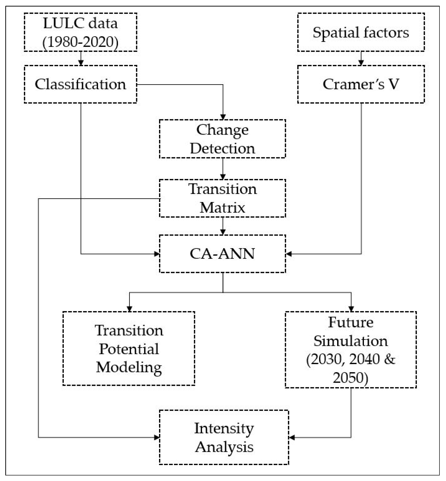
The Greater Bay Area is one of China’s rapidly developing regions and has become an international economic, educational, and technological hub. Under rapid regional socioeconomic development and urban mechanisms, the GBA experienced a transformation that has had a tremendous impact on the spatial pattern of LULC changes [71,72]. In this study, we modeled the spatiotemporal transition potential and future scenario of LULC with the help of the Modules for Land-Use Change Simulation (MOLUSCE) plugin within QGIS software [73,74,75]. The MOLUSCE plugin incorporates some well-known algorithms, such as artificial neural networks (ANNs) and Monte Carlo cellular automata (CA) modeling approaches [76]. We used remote sensing data from 1980 to 2020 with a 10-year interval, spatial variables, DEM, slope [45,77,78], population [45,74], GDP [45], distance from roads [45,78], distance from streams [74], distance from a city [77] and the CA-ANN approach for spatiotemporal transition potential modeling and future LULC simulation for 2030, 2040, and 2050. After the simulation and prediction of LULC, we used an intensity analysis approach at three levels, i.e., interval level, category level and transition level, and further engaged indices to quantify the annual rate of change in LULC classes. Considering all these aspects, we designed our study with the following objectives.

• Modeling spatiotemporal LULC patterns to analyze the magnitude and direction of change over the last 4 decades.
• Predicting future LULC under the influence of physical and socioeconomic factors.
• Identifying current LULC change intensity and potential impacts of LULC change on the spatial pattern.
• Analyzing the predicted LULC intensity scenario.

2. Materials and Methods

2.1. Study Area

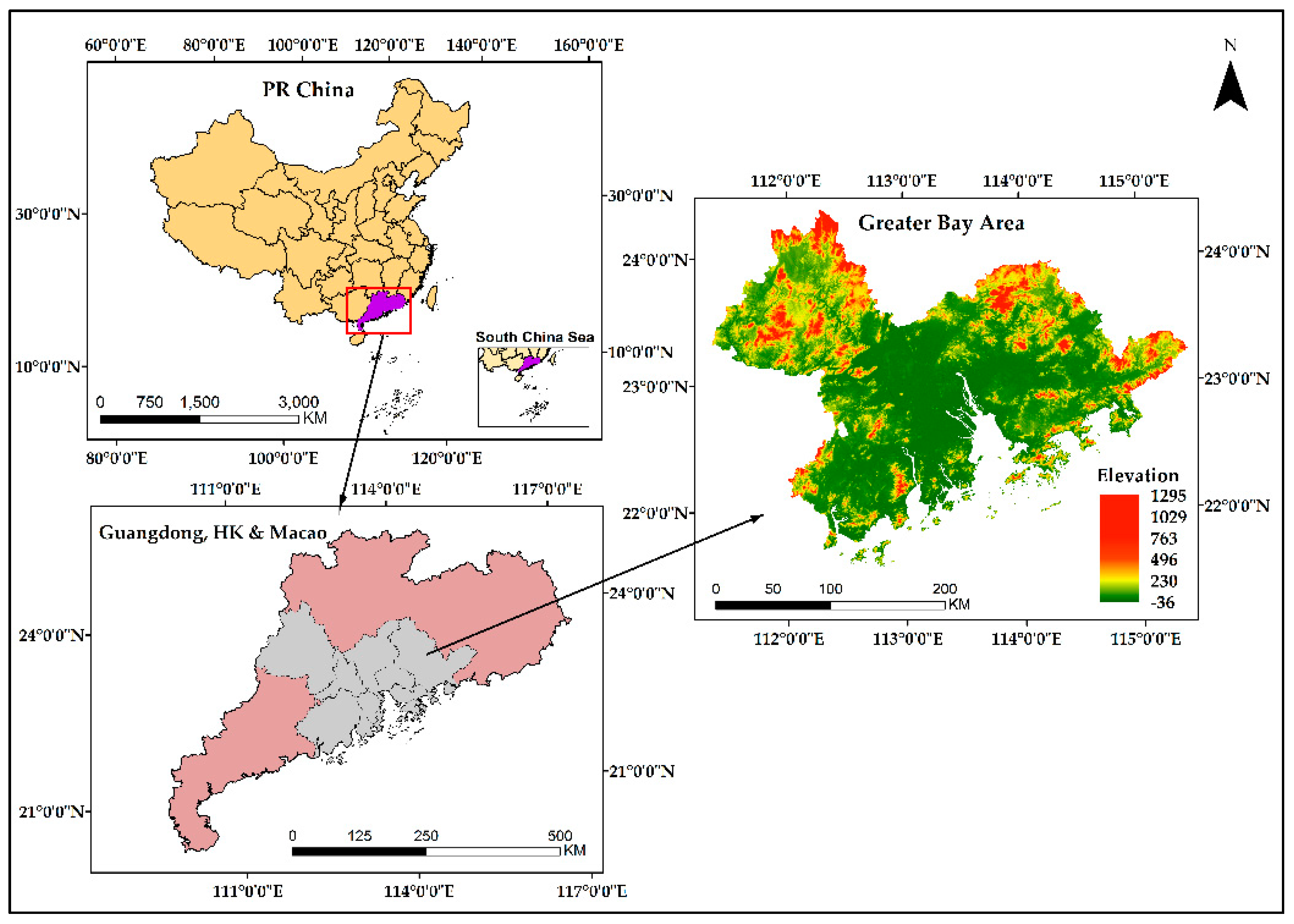
The Guangdong Hong Kong Macao Greater Bay Area, also known as the Pearl River Delta (PRD), is located between 111°–115°–240° E and 22°–25° N (Figure 1) and has a total area of approximately 56,000 km², a population of over 71 million, and a GDP of over 10 trillion RMB [79]. The Guangdong Hong Kong Macao Greater Bay Area is a concept introduced by the Chinese government as a part of the 13th Five-Year Plan for Socioeconomic Development in 2017. The GBA consists of nine cities in Guangdong Province, including Zhaoqing, Foshan, Guangzhou, Dongguan, Jiangmen, Zhongshan, Zhuhai, Shenzhen, Huizhou, and the two Special Administrative Regions (SARs) of Hong Kong and Macao. As one of the largest bay areas in the world, and an economic and industrial symbol of China, the GBA experienced a dramatic LULC change phenomenon and socioeconomic development, especially in terms of the expansion of built-up land and rapid population growth. Rapid urban expansion is mainly attributed to population growth and socioeconomic development. Subsequently, the rapid increase in population and impervious surfaces resulted in many environmental changes in the region [80].

2.2. Data Collection

The LULC data for the Guangdong Hong Kong Macao Greater Bay Area from 1980, 1990, 2000, 2010 and 2020, and the socioeconomic variables, i.e., GDP and population data (1995–2015), were downloaded from the Resources and Environment Science Data Center (RESDC), Chinese Academy of Sciences. China’s land use remote sensing monitoring database is a multitemporal land use database covering the land area of the whole country. Data production is based on temporal Landsat (MSS/TM/ETM+/OLI) images generated through artificial visual interpretation. The data include six primary and 23 secondary land-use types, including arable land, woodland, grassland, water, residential and barren land, with a 30 m spatial resolution. To maintain the accuracy of LULC classification, random sampling methods, GPS field surveys and kappa coefficient tests are engaged. The accuracy rate of cultivated land, urban and rural areas is not less than 95%, and that of grassland, woodland and water area is not less than 90%; that of barren land is not less than 85%. Socioeconomic data are based on national subcounty statistics and the multifactor weight distribution method (www.resdc.cn, accessed on 28 July 2020). The digital elevation model (DEM) was obtained from WorldClim with a spatial resolution of 30 arc-seconds and was derived from the SRTM elevation data (https://www.worldclim.org/, accessed on 16 August 2020). The slope was calculated from the DEM, the road network was obtained from the Socioeconomic Data and Application Center (SEDAC NASA) from 1980 to 2010 (gROADS V1) and the stream network was downloaded from Diva-GIS (https://www.diva-gis.org/, accessed on 16 August 2020). Proximity factors such as distance from roads, distance from streams and distance from the city center, were calculated using the Euclidean distance method in ArcGIS 10.4 (

Table 1. Data Sources.

Category	Description	Year	Source	Accessed on
Multitemporal Data	LULC	1980–2020	https://www.resdc.cn	28 July 2020
Socioeconomic Factors	Population	1995–2015	https://www.resdc.cn	10 August 2020
	GDP	1995–2015
	Road Network	1980–2010	https://sedac.ciesin.columbia.edu
	Distance from Roads		Calculated from road network
	Distance from City		Calculated from city center
Physical Factors	DEM		https://worldclim.org/	16 August 2020
	Slope		Calculated from DEM
	Stream Network		https://www.diva-gis.org/
	Distance from streams		Calculated from stream network

). After data collection, the study area was clipped and projected to WGS_1984_UTM_Zone_49N. Figure 2 represents the methodological workflow of the study.

2.3. Collection of Spatial Variables

Researchers mainly consider the physical and socioeconomic factors responsible for LULC changes, as their contribution to the LULC change mechanism is more significant. Physical factors such as topography and climate are considered the most influential factors that encourage anthropogenic activities [81]. Socioeconomic factors, such as population and GDP, have a potential influence on LULC change [82], and proximity factors, e.g., proximity to roads, distance from the city center and distance from stream network, help in analyzing the driving causes of the landscape pattern [83]. We used a collection of physical, socioeconomic, and proximity factors (Table 1).

The MOLUSCE plugin offers some well-known methods, such as Pearson’s correlation and Cramer’s coefficient, to evaluate the correlation between LULC data and spatial variables. Cramer’s V is a numerical measure of association that ranges from 0 to 1, where 1 indicates a ‘perfect association’ between LULC and the spatial driver and 0 indicates ‘no association’ [15]. The values are not considered ultimate, and they can only help determine whether to include transition potential modeling or not, but generally, a value higher than 0.1 is considered useful [5,84].

2.4. LULC Classification

After extraction and projection of the study area, we grouped the subtypes of land-use data to obtain five categories: urban land, rural settlements, and other construction land as built-up area; woodland, and shrubs as forest; paddy fields, dry land, and cultivated land as cropland; pasture, parks, and green spaces as grassland; and rivers, lakes, reservoirs, and canals as water (

Table 2. LULC classification scheme.

LULC Type	Description
Built-up Area	Impervious surface, residential, commercial and other infrastructure
Forest	All types of forest cover land
Cropland	Agricultural and farmland
Grassland	Parks, green spaces and pasture
Water	Rivers, lakes, ponds and dams

) using the reclassifying tool in ArcGIS 10.4. Furthermore, Google Earth high-resolution images from 2000 were used to interpret and verify the LULC categories. To use the data for transition potential modeling and prediction, we used resampling techniques in ArcGIS to fix the spatial resolution differences between the LULC data and spatial variables.

2.5. Change Analysis and Transition Potential Modeling

We used the Modules for Land-Use Change Simulation (MOULSCE) plugin within QGIS to determine the spatiotemporal changes and calculate the LULC transition between the study intervals (1980 to 1990, 1990 to 2000, 2000 to 2010, and 2010 to 2020) and produced four LULC change maps. Based on the LULC data and explanatory variables, we acquired an area change and transition probability matrix, which comprised rows and columns of landscape categories in the initial and final years. We employed the ANN multilayer perception method for transition potential modeling. The DEM, slope, GDP, population, distance from roads, distance from the city, and distance from streams were employed as explanatory variables (Table 1). These variables are commonly used for LULC change analysis and provide replicable information about the physical and anthropogenic impacts on LULC dynamics.

2.6. Prediction and Model Validation

The purpose of simulation models is to simplify the dynamics of composite urban structures and interpret them in an easily understandable way. We applied the CA-ANN approach within the MOLUSCE plugin for transition potential modeling and future simulation, as many researchers believe that the CA-ANN approach is more potent than linear regression [85,86]. The MOLUSCE plugin effectively computes land-use change analysis [87] and is well suited to analyzing spatiotemporal forest and land-use changes, transition potential modeling and simulating future scenarios [86].

Based on the LULC data of 2000 and 2010, explanatory variables, and transition matrix, we projected the LULC for 2020. To validate the model and prediction accuracy, the MOLUSCE plugin offers a kappa validation technique and comparison of actual and projected LULC images. In the ANN learning process, 100 iterations and a neighborhood value of 3×3 pixels, a learning rate of 0.001, 12 hidden layers, and 0.05 of momentum, were chosen to project the LULC for 2020. After obtaining satisfactory results from the model validation, we employed LULC data from 2010 and 2020 to forecast the LULC in 2030, the LULC of 2000 and 2020 for 2040, and the predicted data for 2030 and 2040 were used to forecast LULC for 2050 (Figure 2).

2.7. Intensity Analysis

Intensity analysis is a statistical framework for expressing variations within various categories over multiple time intervals [88]. This approach analyzes a cross tabulation matrix and examines the transition variation among categories and the persistence of each category across the time intervals. Intensity analysis consists of three-level analysis: interval, category and transition. The interval-level analysis defines the time in which the overall annual change rate is comparatively fast or slow. The category-level analysis examines the changing intensity among LULC categories, and at this level, the intensity of gains and losses for each category are calculated and compared with the uniform intensity. The transition-level analysis compares the changes in terms of size and intensity during each time interval. It compares each category’s gain and loss under the influence of other classes during each time interval. The interval level addresses the question of in which time intervals the annual rate of overall change is relatively fast versus slow, and the category level elaborates which categories are relatively dormant versus active in a given time interval. Based on the above two level analysis, the transition level answer the question of which transitions are intensively avoided versus targeted by a given category in a given time interval [70].

This study used an open-source Microsoft Excel program downloaded from the Intensity Analysis website (https://sites.google.com/site/intensityanalysis/, accessed on 10 August 2020). This program was developed by Safaa Zakaria Aldwaik and Robert Gilmore Pontius Jr., and is based on statistical equations for intensity analysis [70].

We further used the following equation to assess the spatiotemporal magnitude and rate of change in LULC categories:

$$ARC (\%)=\frac{A_2-A_1}{A_1\times t}\times 100$$

(1)

where ARC is the annual rate of change in LULC categories, A₁ and A₂ are the initial and final year areas, respectively, and t is the time interval.

3. Results

3.1. Spatiotemporal Change Analysis

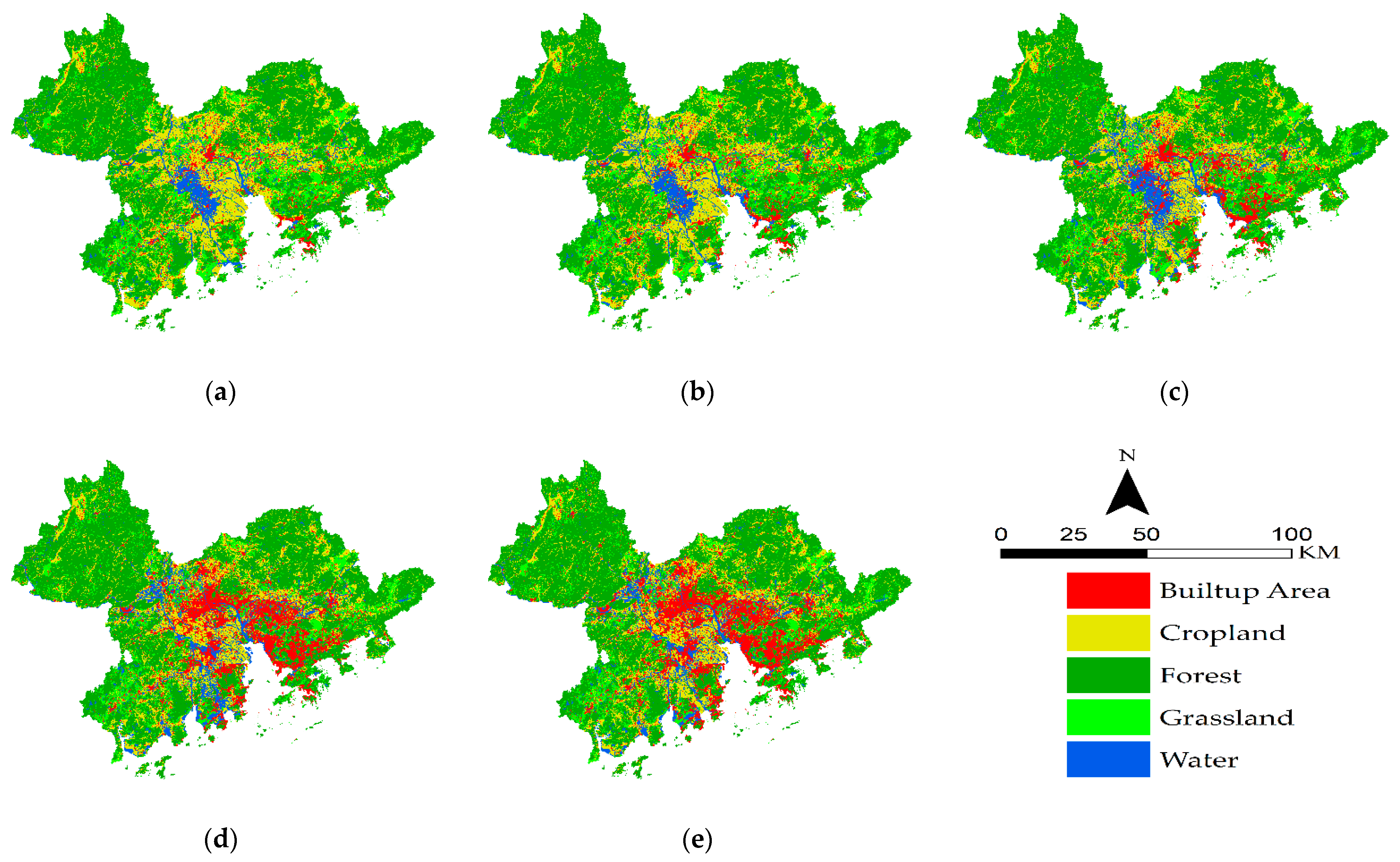
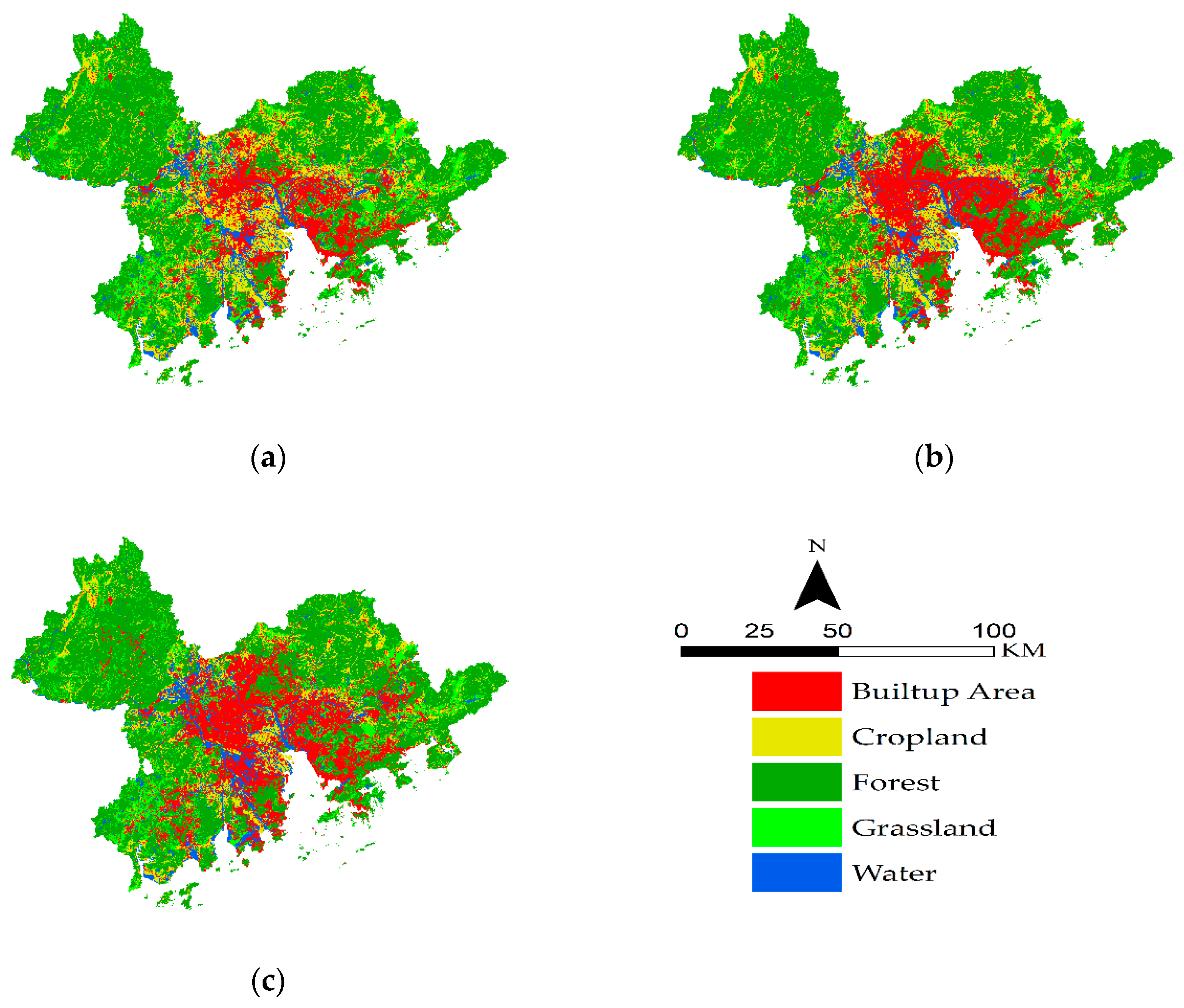
The LULC maps, area statistics and annual rate of change are shown in Figure 3 and

Table 3. LULC area from 1980–2020 (km²) and annual rate of change (ARC).

LULC Type	1980		1990		2000		2010		2020		ARC
	km2	%	km2	%	km2	%	km2	%	km2	%	km2	%
Built-up Area	2600.79	4.75	3072.56	5.59	4520.93	8.22	7237.63	13.16	8114.33	14.75	137.84	5.30
Forest	29,289.12	53.49	29,243.47	53.20	28,865.46	52.49	28,230.72	51.33	27,813.80	50.57	−36.88	−0.13
Cropland	11,967.39	21.85	11,275.30	20.51	10,059.50	18.29	8967.08	16.30	8821.90	16.04	−78.64	−0.66
Grassland	7603.48	13.89	7743.51	14.09	7299.74	13.27	6611.77	12.02	6629.05	12.05	−24.36	−0.32
Water	3299.09	6.02	3629.52	6.60	4244.95	7.72	3949.09	7.18	3618.54	6.58	7.99	0.24

. During the study period, we observed an uneven shift in land use, especially a continuous increase in built-up area from 2600.79 km² to 8114.33 km² (4.75–14.75%), with an annual growth rate of 5.30%; a linear decrease in forest and cropland from 29,289.12 km² to 27,813.80 km² (53.49–50.57%), with an annual decrease rate of −0.13% and −0.66%, respectively, and an area of 11,967.39 km² to 8821.90 km² (21.85–16.04%), respectively. In contrast, grassland and water had mixed results during the study period. Grassland decreased (14.09–12.02%) during 1990–2010, while it increased from 12.02–12.06% during 2010–2020; additionally, water increased from 6.02% to 6.60% during 1980–1990 and from 6.60% to 7.71% during 1990–2000, while it decreased from 7.71% to 7.18% from 2000–2010 and from 7.18% to 6.58% during 2010–2020. The growth and decrease rates during each time interval were different, i.e., during 1980–1990, the urban growth rate was 0.45%, and the forest and cropland decrease rates were 0% and −0.14%, respectively. The grassland and water growth rates were 0.05% and 0.25%, respectively. During the second interval (1990–2000), the urban growth rate was 1.18%, the decreasing rates for forest, cropland, and grassland were −0.03%, −0.27%, and −0.14%, respectively, and the growth rate for water was 0.42%.

During 2000–2010, the urban growth rate was 1.50%, and the decreasing rates for forest, cropland, grassland, and water were −0.05%, −0.27%, −0.24%, and −0.17%, respectively. During 2010–2020, the urban growth was 0.30%, the decreasing rate for forest and cropland was −0.04%, the grassland growth rate was 0.01%, and the water category’s decreasing rate was −0.21%.

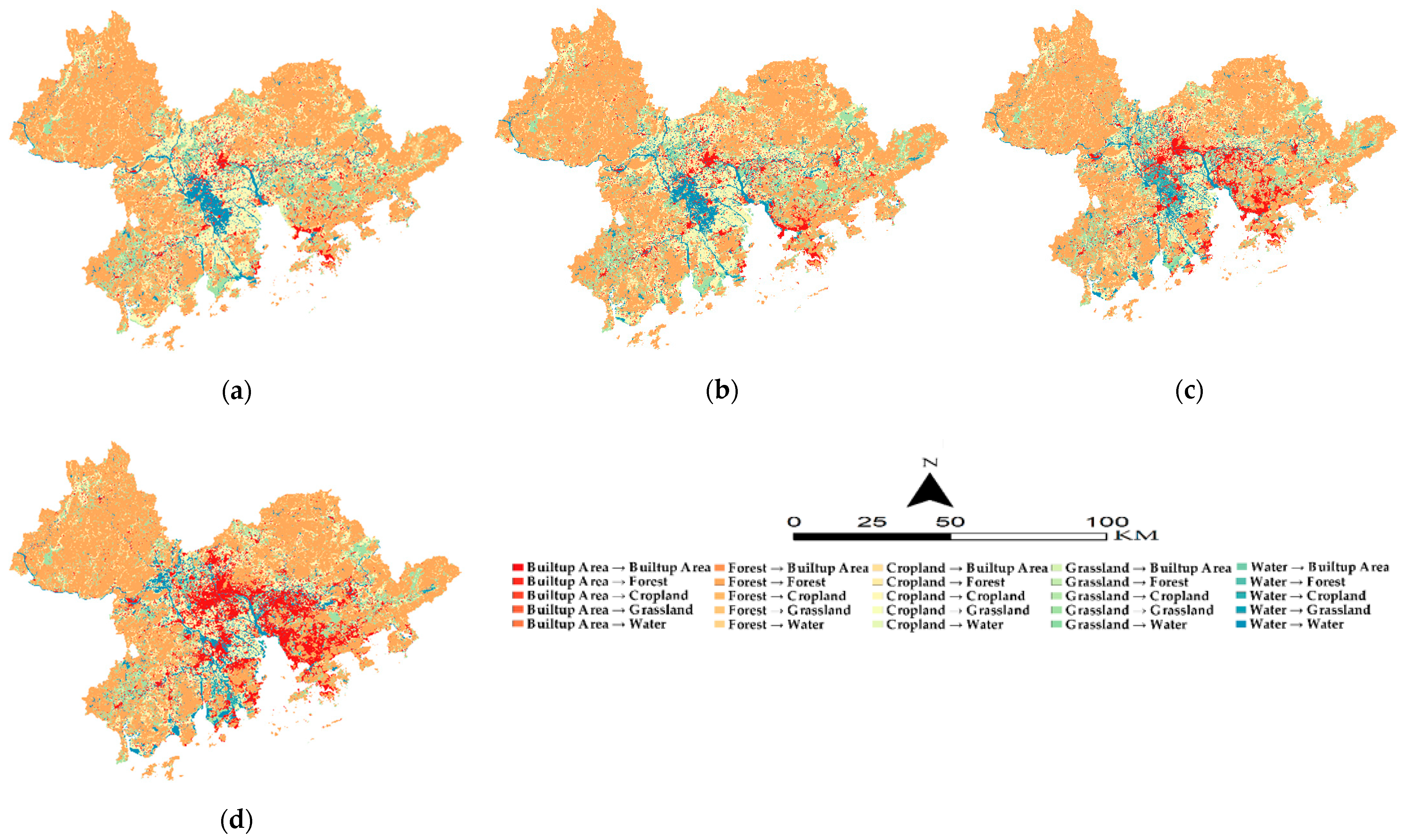
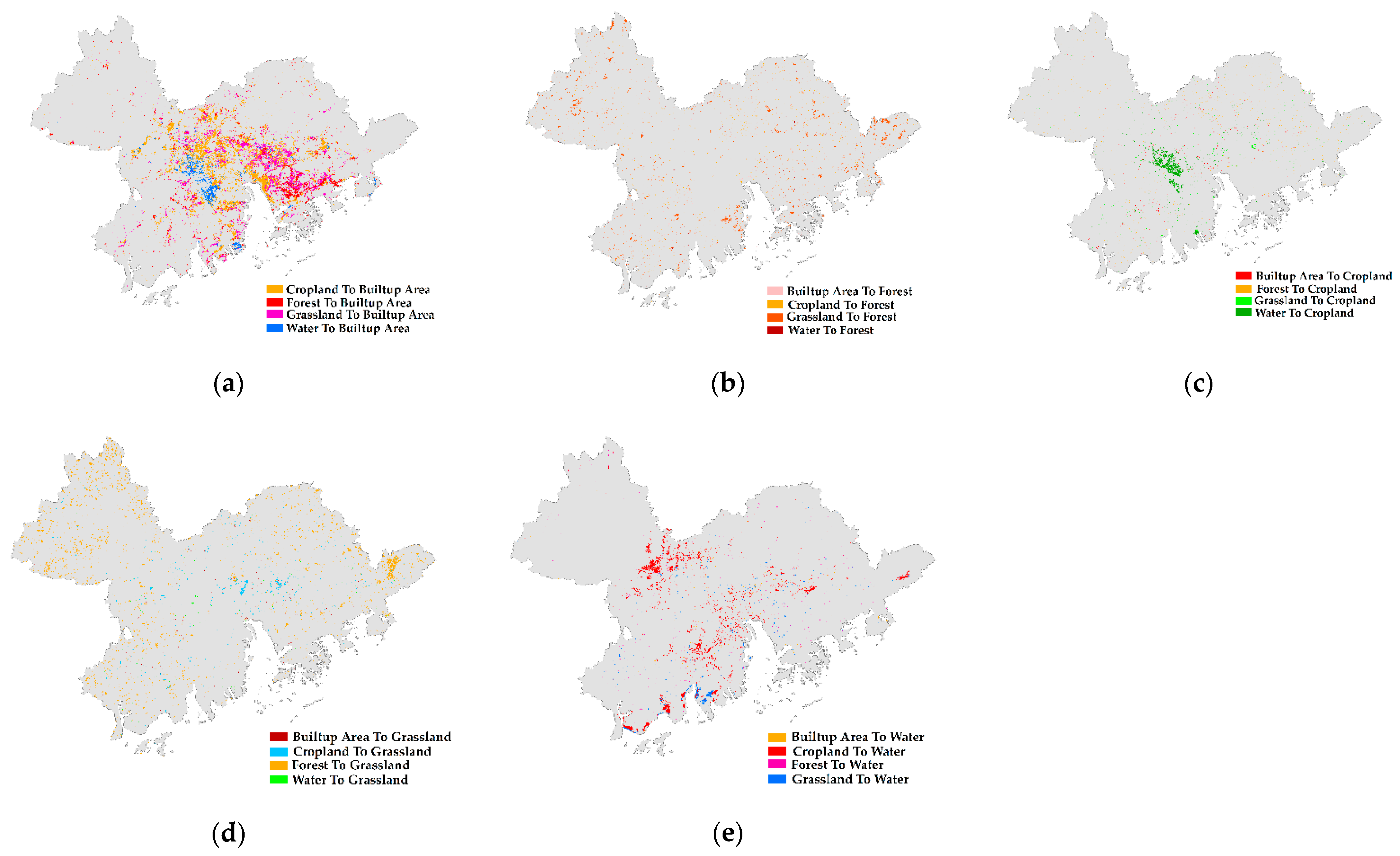
The LULC change analysis explored the spatial dynamic variations in the LULC pattern during the study period. The results from 1980 to 2020 showed a notable expansion in urban areas and a shrinking phenomenon in the forest and cropland. Figure 4 and

Table 4. Temporal changes in 1980–2020.

LULC Category	1980–1990		1990–2000		2000–2010		2010–2020
	km2	%	km2	%	km2	%	km2	%
Built-up Area	471.77	0.84	1448.38	2.63	2716.69	4.94	876.70	1.59
Forest	−45.65	−0.28	−378.01	−0.71	−634.74	−1.16	−416.92	−0.76
Cropland	−692.9	−1.34	−1215.79	−2.22	−1092.42	−1.99	−145.18	−0.26
Grassland	140.03	0.20	−443.77	−0.81	−687.97	−1.25	17.28	0.03
Water	330.43	0.58	615.43	1.12	−295.86	−0.54	−330.55	−0.60

show the spatiotemporal area and percentage change in all LULC categories. Cropland, grassland, forest and water contributed 25.47%, 14.35%, 9.93%, and 5.09% to the built-up area, respectively. Figure 5 and

Table 5. Contribution of LULC categories to change.

LULC Category	Built-Up Area	Forest	Cropland	Grassland	Water
Built-up Area	0.00%	0.52%	0.94%	0.54%	0.48%
Forest	9.93%	0.00%	1.58%	12.07%	0.73%
Cropland	25.47%	1.79%	0.00%	1.77%	9.63%
Grassland	14.35%	7.02%	1.09%	0.00%	1.87%
Water	5.09%	0.46%	4.20%	0.48%	0.00%

represent the inter-transition and contribution of LULC categories to changing phenomena from 1980 to 2020. Cropland was the largest contributor to the change from 1980–2020, with 25.47% to built-up area, 9.63% to water, and 1.79% to forest, while forest contributed 9.93% to built-up area, 1.58% to cropland, 12.07% to grassland and 0.73% to water. Grassland contributed 14.35% to built-up land and 7.02% to forest, and water contributed 5.09% to built-up land and 4.20% to cropland.

3.2. LULC Transition Analysis

The transition matrix plays an essential role in analyzing temporal changes within a set of LULC categories. The rows of the matrix table represent the categories in the initial year, while the columns show the same order of LULC categories in the final year. The diagonal entries show the size of class stability, and each off-diagonal entry represents the size of the transition from one class to different classes. Values close to 1 in diagonal entries represent the stability of a category. Researchers mostly use transition matrices to compare the temporal changes in different regions. To show how each LULC type was projected to change in our study area, we calculated the transition potential matrix with the help of the MOLUSCE plugin during the periods of 1980–1990, 1990–2000, 2000–2010, and 2010–2020 based on the existing LULC conditions and explanatory variables.

Table 6. Transition Matrix from 1980–1990.

Year	1990
1980	Category	Built-Up Area	Forest	Cropland	Grassland	Water
	Built-up Area	0.954	0.008	0.020	0.010	0.007
	Forest	0.003	0.982	0.004	0.011	0.001
	Cropland	0.035	0.009	0.914	0.011	0.032
	Grassland	0.009	0.041	0.008	0.937	0.005
	Water	0.007	0.009	0.022	0.013	0.949

shows the transition potential matrix during 1980–1990, in which built-up area, forest, and water were the most stable categories with probabilities of 0.954, 0.982, and 0.949, respectively, while cropland and grassland decreased with transition probabilities of 0.914 and 0.937, respectively, and contributed 0.035 and 0.009, respectively, to built-up land. During 1990–2000 (

Table 7. Transition Matrix from 1990–2000.

Year	2000
1990	Category	Built-Up Area	Forest	Cropland	Grassland	Water
	Built-up Area	0.930	0.015	0.029	0.017	0.009
	Forest	0.010	0.966	0.007	0.015	0.002
	Cropland	0.060	0.018	0.843	0.010	0.069
	Grassland	0.066	0.038	0.017	0.859	0.019
	Water	0.043	0.016	0.037	0.014	0.890

), the transition values of built-up land and forest were 0.930 and 0.966, respectively, those of cropland and grassland were 0.843 and 0.859, respectively, and that of water was 0.890. Cropland and grassland again contributed 0.060 and 0.066 to the built-up area, respectively. Accordingly, during 2000–2010 (

Table 8. Transition Matrix from 2000–2010.

Year	2010
2000	Category	Built-Up Area	Forest	Cropland	Grassland	Water
	Built-up Area	0.918	0.022	0.026	0.017	0.016
	Forest	0.018	0.949	0.003	0.029	0.002
	Cropland	0.116	0.009	0.809	0.010	0.056
	Grassland	0.123	0.084	0.012	0.761	0.020
	Water	0.119	0.007	0.126	0.012	0.736

), built-up area and forest were stable with values of 0.918 and 0.949, respectively, and cropland, grassland, and water had values of 0.809, 0.761, and 0.736, respectively. Here, cropland, grassland, and water contributed 0.116, 0.123, and 0.119, respectively, of the transition to built-up land. During 2010–2020 (

Table 9. Transition Matrix from 2010–2020.

Year	2020
2010	Category	Built-Up Area	Forest	Cropland	Grassland	Water
	Built-up Area	0.988	0.003	0.002	0.006	0.001
	Forest	0.008	0.984	0.000	0.008	0.000
	Cropland	0.040	0.001	0.958	0.000	0.000
	Grassland	0.034	0.002	0.001	0.961	0.001
	Water	0.035	0.000	0.052	0.002	0.910

), built-up land and forest class areas stabilized again with transition probabilities of 0.988 and 0.984, respectively, and those of cropland and grassland were 0.958 and 0.961, respectively.

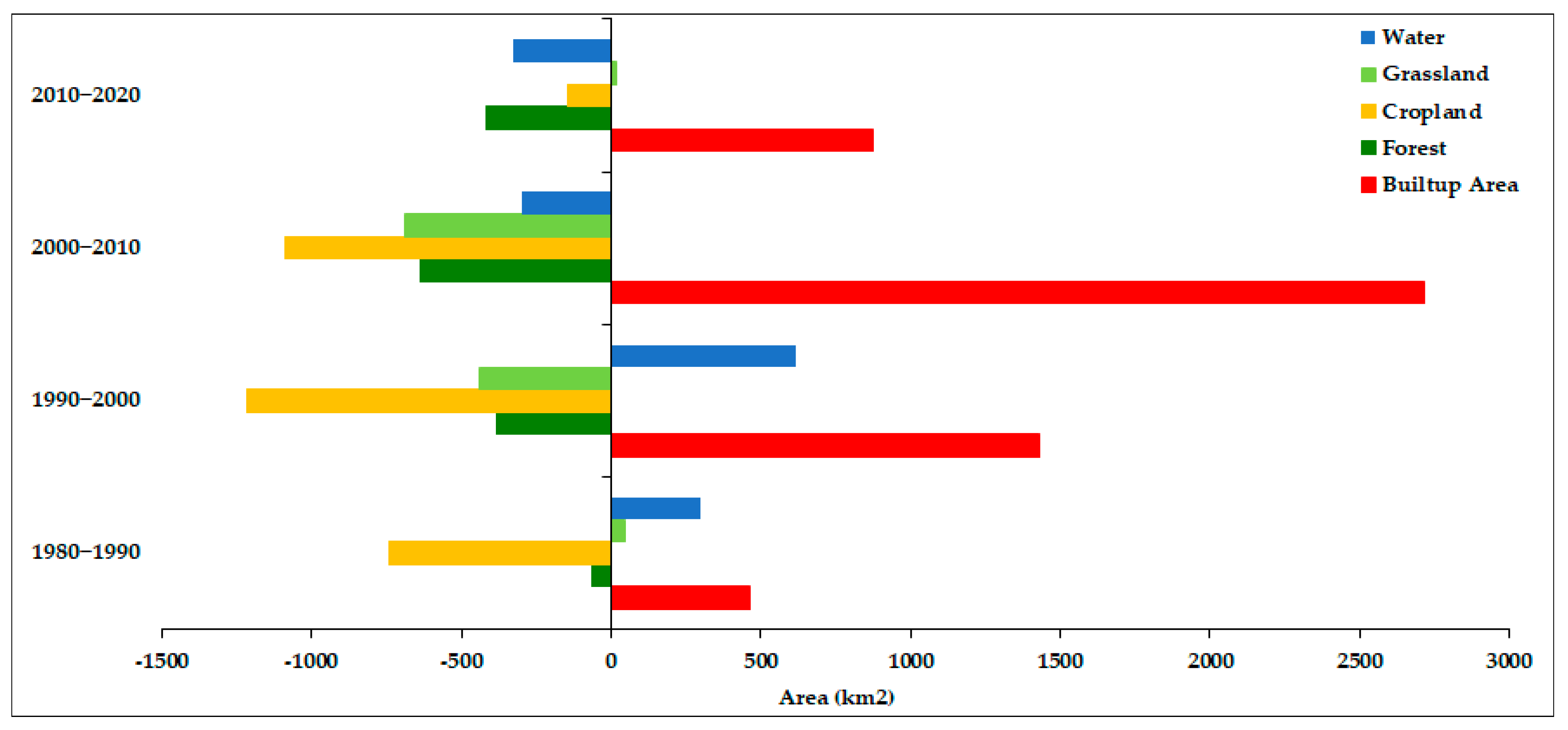
Moreover, as we used LULC data from 2000–2020 along with spatial factors for the prediction of 2040 and the transition probability matrix, the transition matrix between 2000 and 2020 (

Table 10. Transition Matrix from 2000–2020.

Year	2020
2000	Category	Built-Up Area	Forest	Cropland	Grassland	Water
	Built-up Area	0.931	0.018	0.021	0.015	0.015
	Forest	0.025	0.936	0.003	0.035	0.002
	Cropland	0.146	0.009	0.799	0.009	0.036
	Grassland	0.146	0.081	0.012	0.742	0.019
	Water	0.154	0.006	0.122	0.011	0.706

) showed that built-up area and forest were still stable with values of 0.931 and 0.936, respectively, while cropland, grassland and water had fragmentation values of 0.799, 0.742 and 0.706, respectively. During 2030–2040, cropland will still experience a decreasing phenomenon (

Table 11. Transition Matrix from 2030–2040.

Year	2040
2030	Category	Built-Up Area	Forest	Cropland	Grassland	Water
	Built-up Area	0.958	0.013	0.029	0.000	0.000
	Forest	0.003	0.997	0.000	0.000	0.000
	Cropland	0.187	0.001	0.808	0.000	0.004
	Grassland	0.009	0.000	0.007	0.973	0.012
	Water	0.018	0.000	0.002	0.001	0.978

), while other classes will show comparatively stable behavior.

Table 12. Transition Matrix from 2040–2050.

Year	2050
2040	Category	Built-Up Area	Forest	Cropland	Grassland	Water
	Built-up Area	1.00	0.00	0.00	0.00	0.00
	Forest	0.00	1.00	0.00	0.00	0.00
	Cropland	0.27	0.00	0.732	0.00	0.00
	Grassland	0.00	0.00	0.00	1.00	0.00
	Water	0.00	0.00	0.00	0.00	0.998

represents the transition probability matrix during 2040–2050. Here, we observed that built-up land, forest, grassland, and water were the most stable categories, with transition values of 1.0, 1.0 1.0, and 0.99, respectively, while cropland will experience rapid fragmentation, with a value of 0.732. During the study period, along with the built-up area, the forest was stable because of the conservation, afforestation, and reforestation policy of the Chinese government, but the significant pressure was on cropland, which donated the largest share to other LULC categories.

Table 13. Gains and losses of each category (km²).

Category	1980–1990	1990–2000	2000–2010	2010–2020
Built-up Area	459.66	1428.18	2714.59	875.79
Forest	−61.92	−384.43	−635.45	−417.13
Cropland	−739.72	−1216.14	−1092.54	−145.17
Grassland	45.85	−441.56	−688.83	17.23
Water	296.13	613.95	−297.76	−330.72

and Figure 6 elaborate the gained and lost areas of each category over each time interval.

3.3. Selection of Spatial Variables

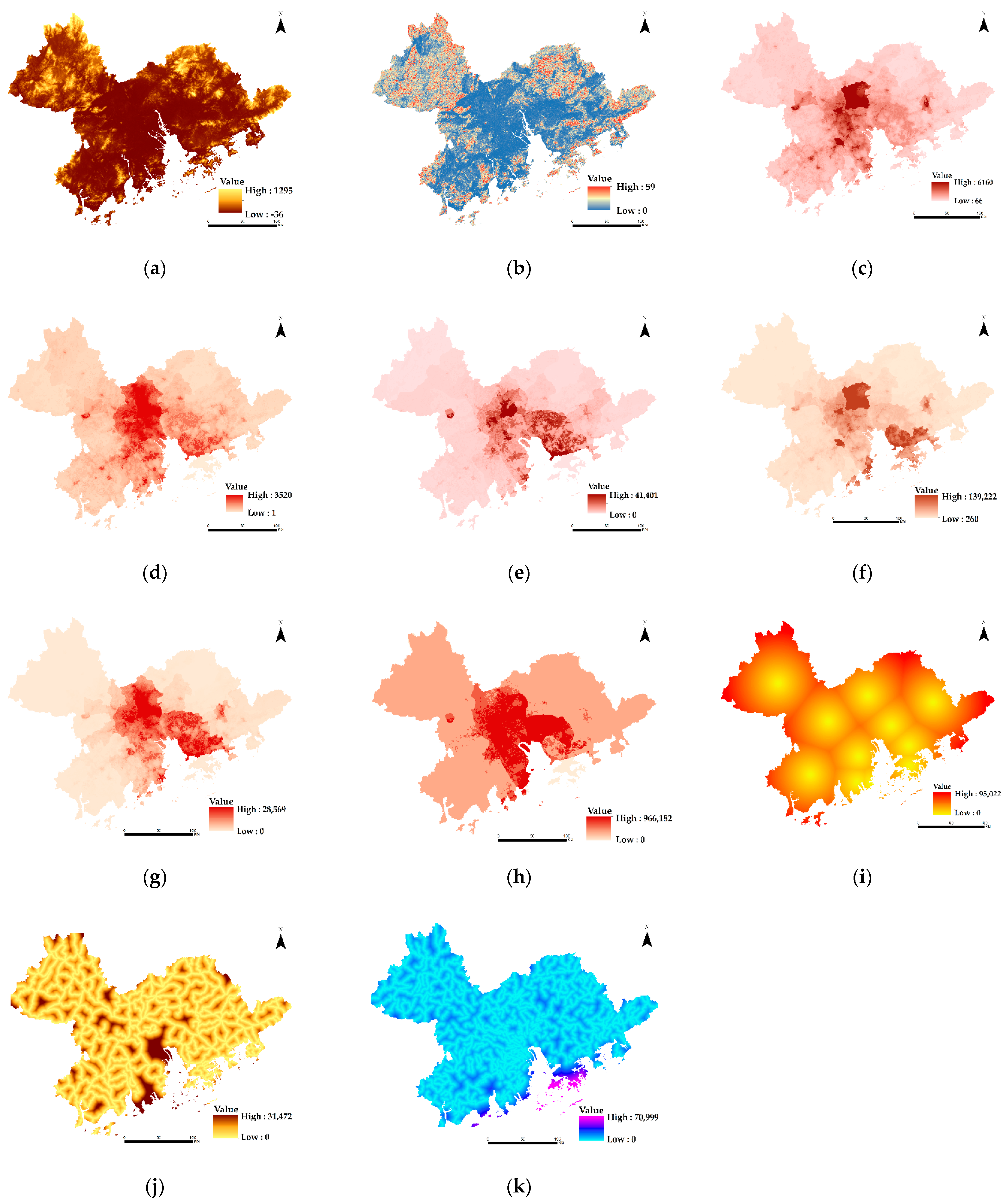
According to transition matrix analysis, we observed that the significant growth in built-up land was mainly due to cropland fragmentation. All these transitions were based on physical and socioeconomic driving factors. Researchers mostly use these spatial factors to investigate LULC dynamics.

Table 14. Cramer’s V value of spatial variables.

Spatial Variables	Cramer’s V
DEM	0.35
Slope	0.33
Population	0.30
GDP	0.28
Distance from City	0.15
Distance from Roads	0.12
Distance from Streams	0.08

shows the prospective Cramer’s V value of each spatial variable. The Cramer’s V value suggests that the variables are ideal for transition potential modeling, as their values are more significant. According to the values, the selection of physical and socioeconomic explanatory variables is more effectual, i.e., DEM: 0.35; slope: 0.33; population: 0.30; and GDP: 0.28. Figure 7 shows the spatial variables used in this study.

3.4. Transition Potential Modeling and Model Validation

The MOLUSCE plugin integrates some well-known algorithms for transition potential modeling, such as the ANN (multilayer perception), weights of evidence, multicriteria evaluation, logistic regression, and CA algorithm, for future simulation. The spatial variables for model calibration were chosen based on their relatively strong association with LULC, as measured by Cramer’s coefficient.

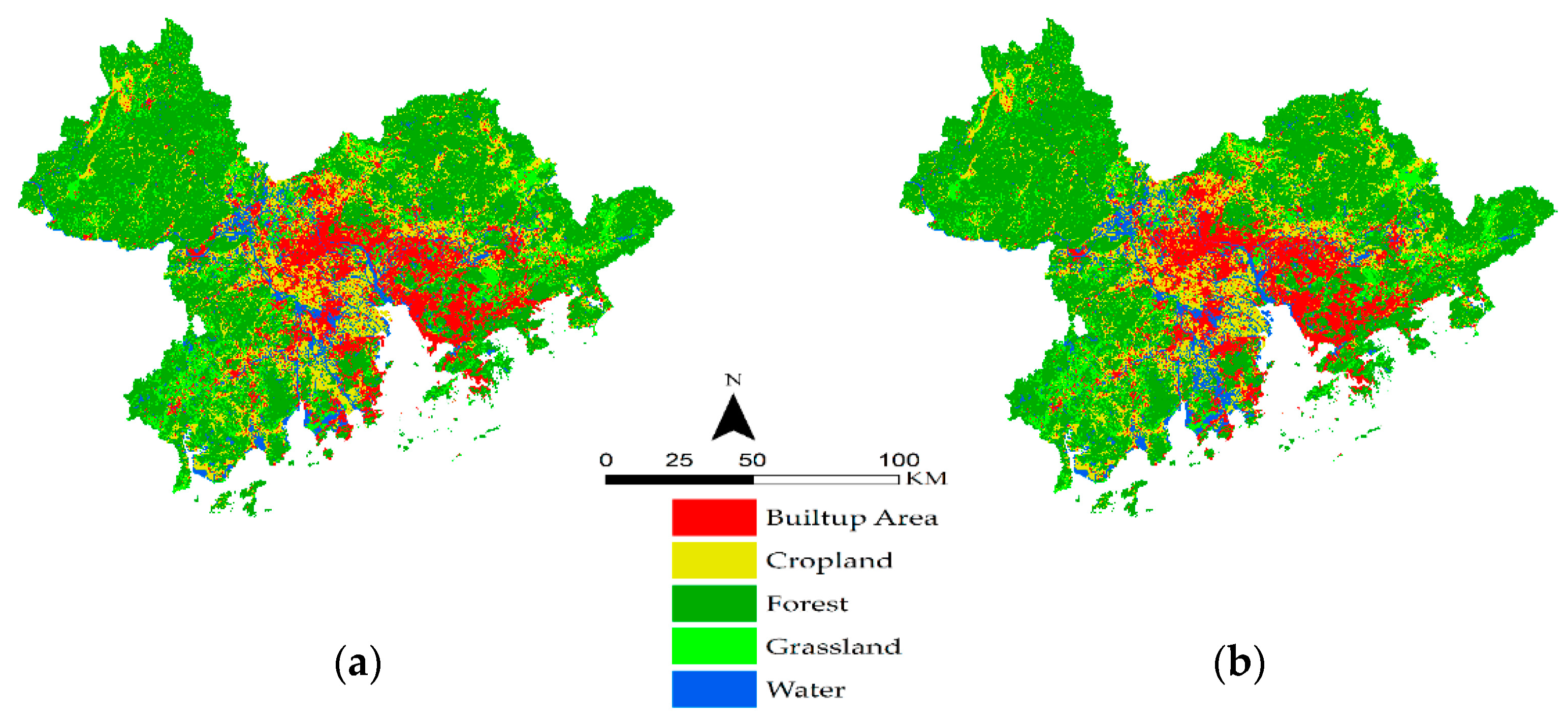
We used the CA-ANN approach for transition potential modeling and prediction. We employed LULC data from 2000–2010 along with spatial variables to projected LULC for 2020 and obtained a validation kappa value of 0.76. After obtaining the projected LULC, we compared the actual LULC of 2020 with the projected data and obtained an overall accuracy of 96.25% and an overall kappa value of 0.94. Figure 8 and

Table 15. Actual and projected LULC of 2020.

LULC Category	Actual		Projected		Accuracy	Kappa Value
	km2	%	km2	%		ANN	Validation
Built-up Area	8114.33	14.75	7681.33	13.97	96.25%	0.77	0.94
Forest	27,813.80	50.57	28,427.66	51.69
Cropland	8821.90	16.04	8964.28	16.30
Grassland	6629.05	12.05	6001.82	10.91
Water	3618.54	6.58	3921.20	7.13

show the actual and forecasted maps and statistics for 2020.

3.5. Prediction of LULC

After obtaining satisfactory results from model validation, we predicted the LULC for 2030, 2040 and 2050. We employed the temporal LULC data from 2010 and 2020, the spatial variables, and the transition probability matrix (Table 9) to predict the LULC for 2030 and obtained a kappa value of 0.95. Furthermore, the LULC of 2000 and 2020, including the explanatory variables and transition matrix (Table 10), were used for the prediction of 2040, and we obtained a kappa value of 0.78. Finally, we predicted the LULC for 2050 based on the projected data for 2030–2040 and the transition matrix (Table 11) and obtained a kappa value of 0.91. Figure 9 and

Table 16. Predicted area statistics (2030, 2040 and 2050).

Category	2030			2040			2050
	km2	%	Kappa	km2	%	Kappa	km2	%	Kappa
Built-up Area	8119.53	14.76	0.95	9909.48	18.02	0.78	11,642.31	21.17	0.91
Forest	27,812.45	50.57		28,549.20	51.91		27,832.26	50.61
Cropland	8858.20	16.11		7956.07	14.47		5460.55	9.93
Grassland	6628.51	12.05		5126.01	9.32		6452.83	11.73
Water	3578.92	6.51		3456.85	6.29		3609.67	6.56

represent the map, area statistics, and overall validation kappa of the predicted LULC of 2030, 2040, and 2050.

3.6. Intensity Analysis

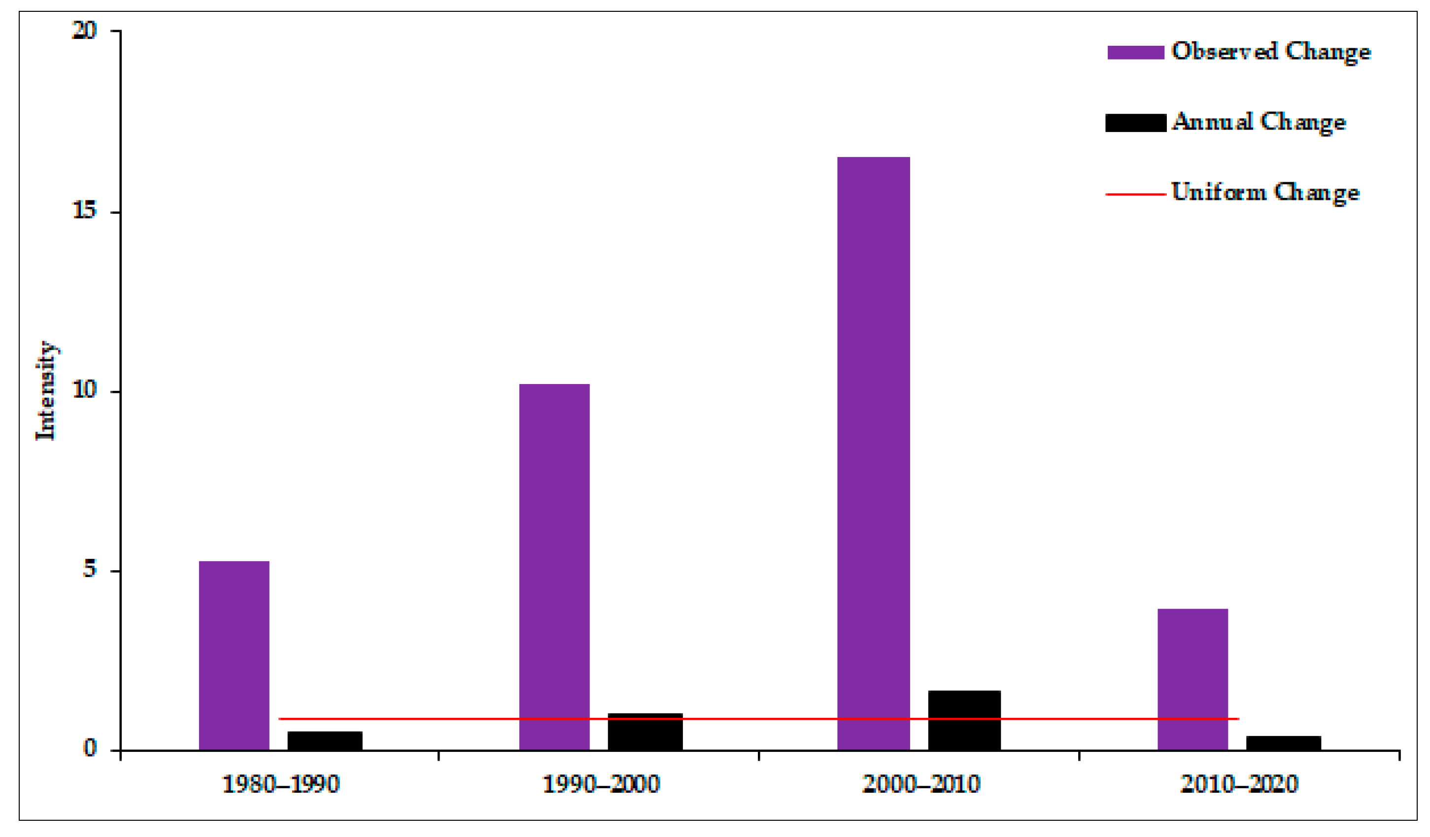
After change detection, transition analysis and prediction, we analyzed the change in terms of intensity at three levels, i.e., interval level, category level, and transition level [70].

Table 17. Interval-level Change Intensity.

Interval	Observed Change	Annual Change Intensity	Uniform Change Intensity
1980–1990	5.28	0.53	0.90
1990–2000	10.23	1.02	0.90
2000–2010	16.54	1.65	0.90
2010–2020	3.96	0.40	0.90

and Figure 10 show the change intensity at the interval level in which we observed that the uniform intensity was 0.90. The annual changes during 1980–1990 and 2010–2020 were smaller than the uniform intensity, i.e., 0.53 and 0.40, indicating that the change intensity was slow compared with the uniform intensity. During the second and third intervals (1990–2000 and 2000–2010), the annual change intensity was greater than the uniform change intensity, which supported the fast change during these intervals.

We analyzed each category’s intensity in category-level analysis and compared the gain and loss intensity with the uniform intensity during each interval.

Table 18. Category-level Gain Intensity.

Interval	1980–1990		1990–2000		2000–2010		2010–2020
Category	Gain Intensity	Uniform Intensity	Gain Intensity	Uniform Intensity	Gain Intensity	Uniform Intensity	Gain Intensity	Uniform Intensity
Built-up Area	0.53	0.53	1.62	1.02	2.9	1.65	1.07	0.4
Forest	0.65	0.53	0.83	1.02	1.14	1.65	0.06	0.4
Cropland	0.55	0.53	0.96	1.02	1.71	1.65	0.54	0.4
Grassland	0.46	0.53	0.62	1.02	0.82	1.65	0.16	0.4
Water	0.45	0.53	1.00	1.02	1.13	1.65	0.03	0.4

represents the gains and uniform intensity of each category during each interval. Except for the first interval, the built-up area had the largest size compared with uniform intensity and other categories, which indicated the fast gain in the built-up area as a result of the fragmentation of other categories.

Table 19. Category-level Loss Intensity.

Interval	1980–1990		1990–2000		2000–2010		2010–2020
Category	Loss Intensity	Uniform Intensity	Loss Intensity	Uniform Intensity	Loss Intensity	Uniform Intensity	Loss Intensity	Uniform Intensity
Built-up Area	0.46	0.53	0.7	1.02	0.82	1.65	0.12	0.4
Forest	0.18	0.53	0.34	1.02	0.51	1.65	0.16	0.4
Cropland	0.86	0.53	1.57	1.02	1.91	1.65	0.42	0.4
Grassland	0.63	0.53	1.41	1.02	2.39	1.65	0.39	0.4
Water	0.51	0.53	1.10	1.02	2.64	1.65	0.90	0.4

shows the category-level loss intensity. During the first and second intervals, the loss intensity value of cropland was the highest (0.86 and 1.57, respectively), while during the third interval, cropland, grassland and water lost the most, as their lost intensities were larger than uniform intensity, with values of 1.91, 2.39, and 2.64, respectively. During the final interval, the cropland, grassland, and water intensities were greater than uniform intensity, which indicated a fast fragmentation in these categories and eventually the contribution to other categories, especially to built-up area, which was further described in the transition-level intensity section.

Table 20. Transition to Built-up Area.

Interval	1980–1990		1990–2000		2000–2010		2010–2020
Category	Transition Intensity	Uniform Intensity	Transition Intensity	Uniform Intensity	Transition Intensity	Uniform Intensity	Transition Intensity	Uniform Intensity
Forest	0.03	0.13	0.10	0.45	0.18	0.94	0.08	0.30
Cropland	0.35	0.13	0.60	0.45	1.16	0.94	0.40	0.30
Grassland	0.09	0.13	0.66	0.45	1.23	0.94	0.34	0.30
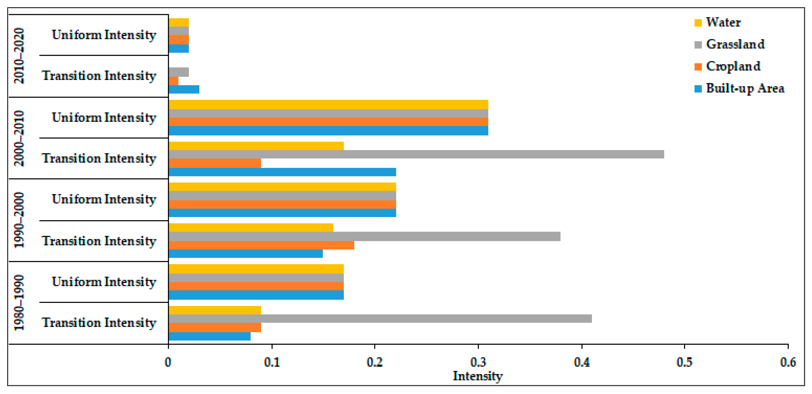
Water	0.07	0.13	0.43	0.45	1.19	0.94	0.35	0.30

and Figure 11 show the transition of other categories to built-up area during the study period. Overall, cropland and grassland contributed the most considerable amounts to built-up area. During the first interval transition, the intensity of cropland was 0.35, and the uniform intensity was 0.13. Hence, the transition intensity was greater than the uniform intensity, indicating fast fragmentation of cropland to built-up area. During 1990–2000, cropland and grassland transition intensities were greater than those of other categories, i.e., 0.60 and 0.66, respectively, while the uniform intensity during this period was 0.45. During 2000–2010, the uniform intensity was 0.94, and the cropland, grassland, and water transition intensities were 1.16, 1.23, and 1.19, respectively. During the last interval, the uniform intensity was 0.30, and the transition intensities of cropland, grassland, and water were 0.40, 0.34, and 0.35, respectively. Therefore, the gain in built-up land from cropland means that cropland’s transition intensity was greater than the uniform intensity during the study period.

Table 21. Transition to Forest.

Interval	1980–1990		1990–2000		2000–2010			2010–2020
Category	Transition Intensity	Uniform Intensity	Transition Intensity	Uniform Intensity	Transition Intensity	Uniform Intensity	Transition Intensity	Uniform Intensity
Built-up Area	0.08	0.17	0.15	0.22	0.22	0.31	0.03	0.02
Cropland	0.09	0.17	0.18	0.22	0.09	0.31	0.01	0.02
Grassland	0.41	0.17	0.38	0.22	0.48	0.31	0.02	0.02
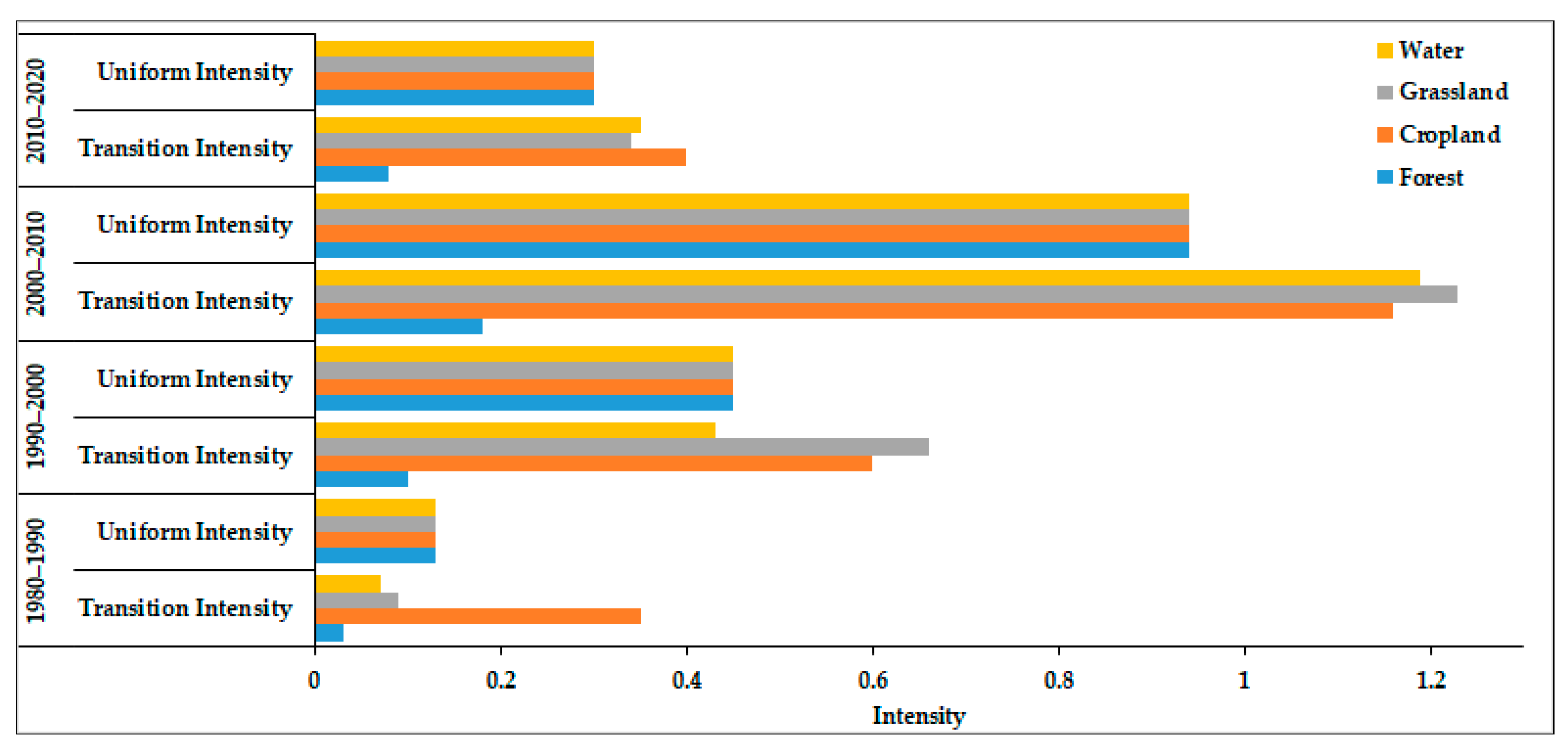
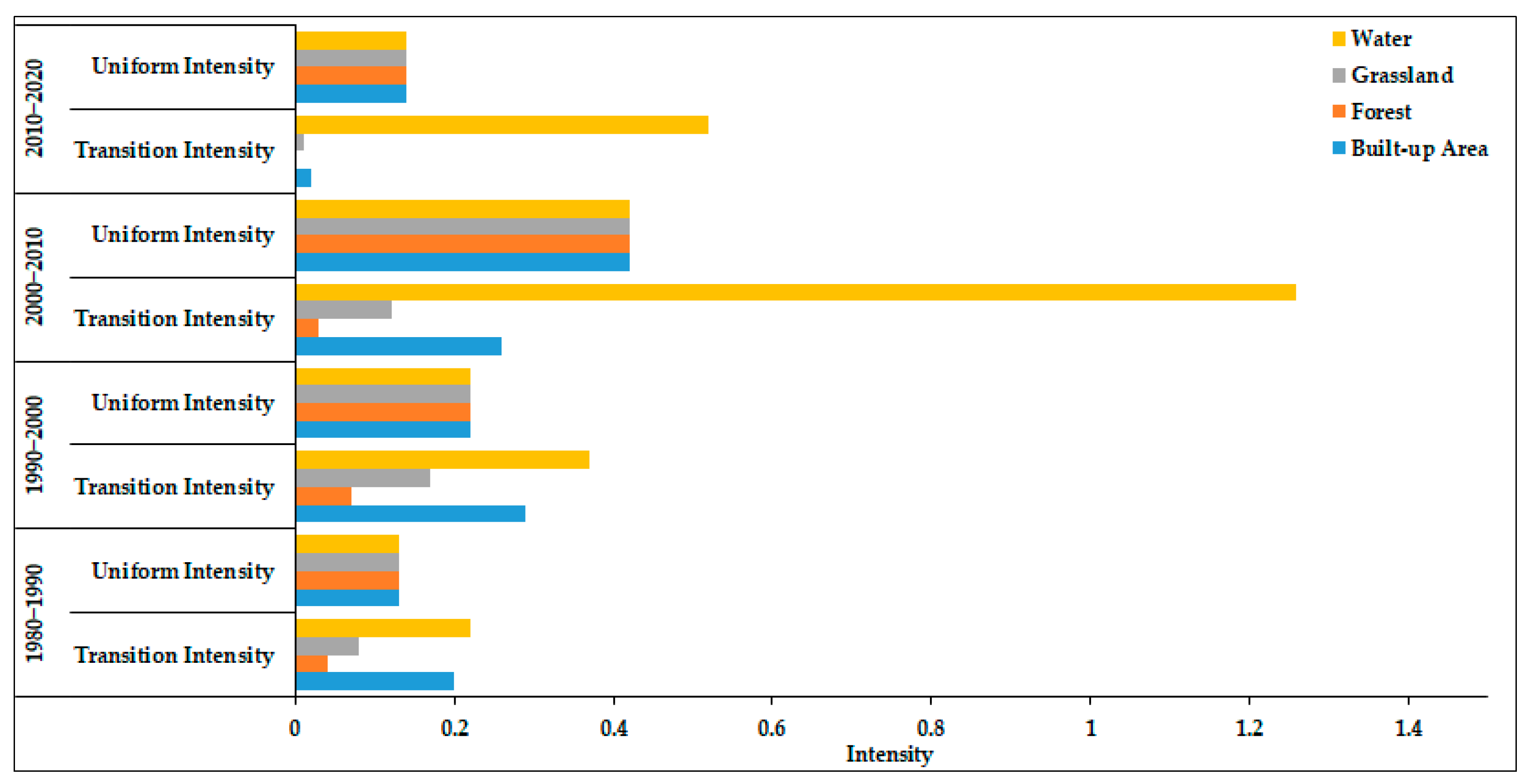
Water	0.09	0.17	0.16	0.22	0.17	0.31	0.00	0.02

and Figure 12 represent the size of transition intensity of other categories to forest against the uniform intensity, indicating that grassland contributed more than the other classes to forest during the first three intervals. In contrast, during the last interval, the built-up area donated more than the other categories. During the first three intervals, the grassland transition intensity was 0.41, 0.38, and 0.48, respectively, and the uniform intensity was 0.17, 0.22, and 0.31, respectively. During 2010–2020, the built-up land and grassland transition intensities were 0.03 and 0.02, respectively, while the uniform intensity was 0.02. Hence, forest gains would cause a transition in grassland as grassland donated more than the other categories.

Table 22. Transition to Cropland.

Interval	1980–1990		1990–2000		2000–2010		2010–2020
Category	Transition Intensity	Uniform Intensity	Transition Intensity	Uniform Intensity	Transition Intensity	Uniform Intensity	Transition Intensity	Uniform Intensity
Built-up Area	0.20	0.13	0.29	0.22	0.26	0.42	0.02	0.14
Forest	0.04	0.13	0.07	0.22	0.03	0.42	0.00	0.14
Grassland	0.08	0.13	0.17	0.22	0.12	0.42	0.01	0.14
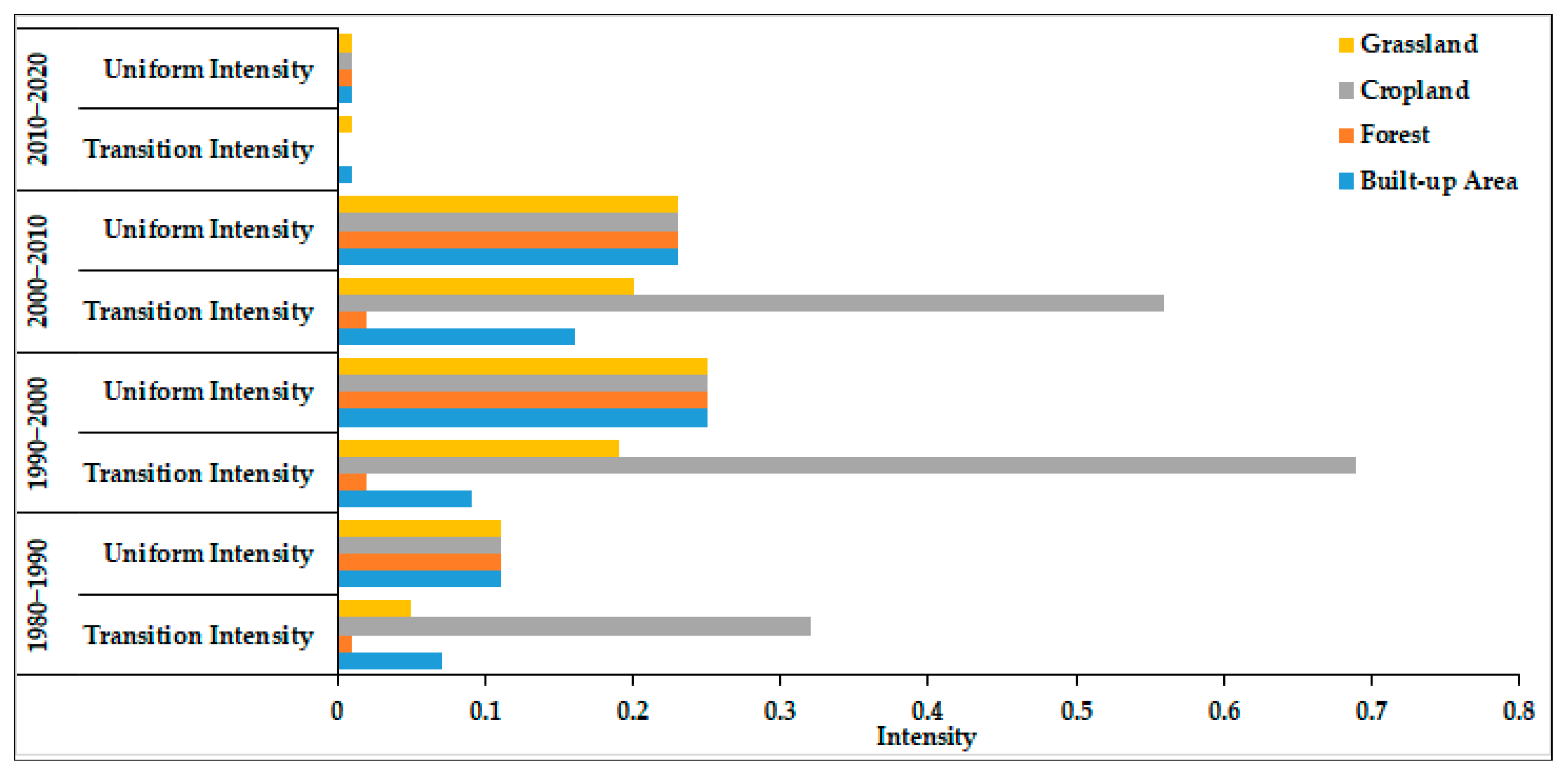
Water	0.22	0.13	0.37	0.22	1.26	0.42	0.52	0.14

and Figure 13 show the transition intensity of other categories to cropland. We observed that the water transition intensity was more significant than the uniform intensity throughout the study period, i.e., 0.22, 0.37, 1.26 and 0.52, while the uniform intensity was 0.13, 0.22, 0.42 and 0.52, respectively.

Table 23. Transition to Water.

Interval	1980–1990		1990–2000		2000–2010		2010–2020
Category	Transition Intensity	Uniform Intensity	Transition Intensity	Uniform Intensity	Transition Intensity	Uniform Intensity	Transition Intensity	Uniform Intensity
Built-up Area	0.07	0.11	0.09	0.25	0.16	0.23	0.01	0.01
Forest	0.01	0.11	0.02	0.25	0.02	0.23	0.00	0.01
Cropland	0.32	0.11	0.69	0.25	0.56	0.23	0.00	0.01
Grassland	0.05	0.11	0.19	0.25	0.20	0.23	0.01	0.01

and Figure 14 show the transition to water from other categories. During the first three intervals, cropland’s transition intensity was more significant than the uniform intensity, which indicated that the transition of cropland to water was faster than other categories, i.e., 0.32, 0.69 and 0.56, respectively, while the uniform intensity was 0.11, 0.25 and 0.23, respectively. During the last interval, as we discussed earlier, the water size decreased, so the other categories did not contribute to water.

Table 24. Interval-level Change Intensity (2030–2050).

Interval	Observed Change	Annual Change Intensity	Uniform Change Intensity
2030–2040	5.72	0.57	0.56
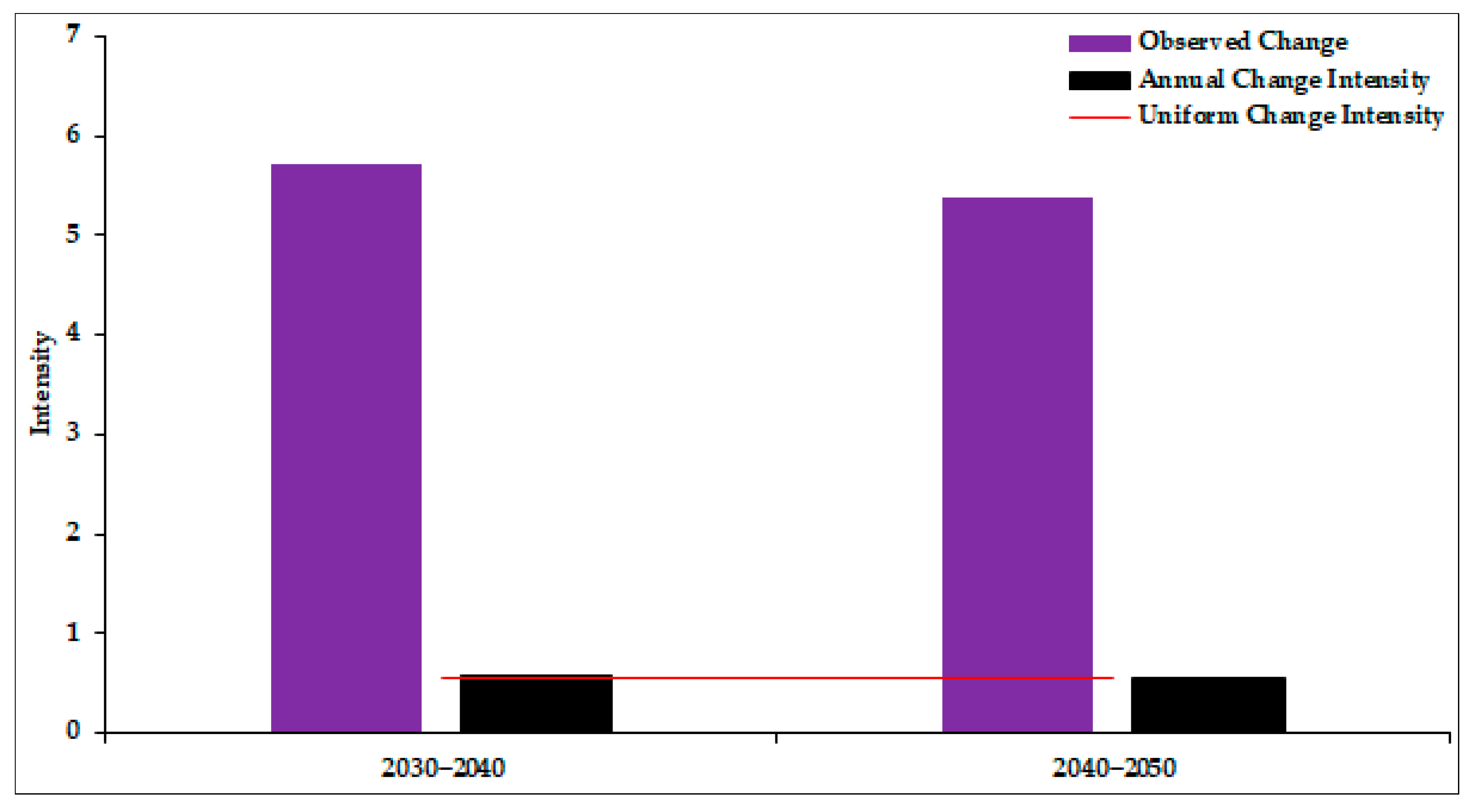
2040–2050	5.39	0.54	0.56

and Figure 15 represent the expected change intensity during 2030–2050. According to the results, during 2030–2040, the annual change intensity was greater than the uniform change intensity, i.e., 0.57 and 0.56, respectively, while during 2040–2050 the annual change intensity was smaller than the uniform intensity (0.54 and 0.56, respectively). The observed change during 2030–2040 was 5.72 and that during 2040–2050 was 5.39.

Table 25. Category-level Gain Intensity.

Interval	2030–2040		2040–2050
Category	Gain Intensity	Uniform Intensity	Gain Intensity	Uniform Intensity
Built-up Area	1.85	0.57	2.12	0.54
Forest	0.14	0.57	0.00	0.54
Cropland	0.45	0.57	0.00	0.54
Grassland	0.01	0.57	0.00	0.54
Water	0.16	0.57	0.00	0.54

and

Table 26. Category-level Loss Intensity.

Interval	2030–2040		2040–2050
Category	Loss Intensity	Uniform Intensity	Loss Intensity	Uniform Intensity
Built-up Area	0.42	0.57	0.00	0.54
Forest	0.03	0.57	0.00	0.54
Cropland	1.92	0.57	2.68	0.54
Grassland	0.27	0.57	0.00	0.54
Water	0.22	0.57	0.02	0.54

show the gain and loss intensity at the category level. According to the projected results, our study area will experience a rapid expansion in built-up area in the future, i.e., the gain intensity of the built-up area will be greater than the uniform intensity during both intervals (1930–1940 and 1940–1950). The uniform intensity during 2030–2040 and 2040–2050 will be 0.57 and 0.54, respectively, while the built-up area’s gain intensity will be 1.85 and 2.12, respectively. Accordingly, cropland will still experience rapid fragmentation in the future. During 2030–2040, the loss intensity of cropland will be 1.92 against a uniform intensity of 0.57, while during 2040–2050, cropland will experience a loss intensity of 2.68 against a uniform intensity of 0.54.

4. Discussion

Unprecedented urban expansion has transformed the natural environment and landscape patterns worldwide, especially in the twenty-first century [89]. Physical and socioeconomic factors such as geography, population and economic growth are considered the most significant driving forces of urbanization [3]. However, socioeconomic development has a greater impact on urban expansion than population growth [90]. The extent and pace of urban expansion and fragmentation of landscape patterns have led to concerns about climatic changes, food security and scarcity of natural resources.

LULC changes are closely linked to geographical location and development policies. After the ‘opening up’ policy of China in the late 1970s, the economic reforms resulted in massive migration, immigration and urban expansion, especially in the southern part of the country. Based on the spatiotemporal LULC data and physical and socioeconomic driving factors, we analyzed the change from 1980 to 2020 and created a transition probability matrix for each interval using the MOLUSCE plugin within QGIS software. Furthermore, with the help of the CA-ANN multilayer perception approach within the MOLUSCE plugin, we projected the LULC for 2030, 2040, and 2050.

Our results indicate that physical and socioeconomic factors significantly affected landscape patterns during the study period. Generally, areas with lower elevations are associated with rapid LULC changes, as the geography of such areas is more suitable for anthropogenic activities. The highest changes occurred in the plain areas of the GBA, especially along the coast of the Pearl River, as the slope of this part is comparatively lower than that of other parts. The northern, eastern, and western portions, which consist of mountains, hills, and forest, do not experience rapid fragmentation.

The concept of GBA embodies broader goals to achieve market-oriented reforms and cooperation among the eleven cities in the socioeconomic sector, education, innovation, international business, and technological advancement. According to the “Outline Development Plan for the Guangdong-Hong Kong-Macao Greater Bay Area”, by 2035, the GBA will become a globally competitive modern economic and industrial system; however, increasing the population and scarcity of land resources is one of the major challenges in the GBA [79]. Many studies have indicated that population growth and economic development are the driving forces of built-up expansion [91]. The increasing built-up area negatively impacts the natural environment, water quality and biodiversity [14]. According to our results, the GBA has experienced a dramatic conversion of LULC during the last four decades, especially in the rapid transition of cropland into built-up area. From 1980 to 2020, the built-up area increased from 4.75% to 14.75%, and cropland contributed 25.47%, grassland contributed 14.35%, forest contributed 9.93% and water bodies contributed 5.09%. Additionally, the future simulation results endorse that built-up land will continue to increase from 2030 to 2050 with percentages of 14.76% to 21.17%, and cropland will continue to decrease from 16.11% to 9.93%.

Furthermore, intensity analysis helps in analyzing and understanding the size and intensities of the transition at the interval, category, transition levels and the change patterns [70]. In this study, the intensity analysis reflected the rapid transition phenomenon in the LULC categories during past and future scenarios. During the first and fourth time intervals, the rate of annual change intensity was slower than that during the second and third time intervals, which indicated that the impacts of socioeconomic driving factors during the four decades were different. Furthermore, except for the first time interval, the gain intensity in the built-up area was more significant than the uniform intensity. The loss intensity of cropland was greater than the uniform intensity, which supports the result that the overall gain in the built-up area and the overall loss in cropland were greater than other categories. Similarly, the transition intensity of cropland to built-up area was greater than the uniform intensity. Hence, the gain in built-up area targets cropland more than other categories throughout the study period.

Ultimately, the drastic changes in LULC, especially urban sprawl and cropland fragmentation, could endanger natural resources, the environment, and food security. Therefore, the spatiotemporal and projected LULC simulation results will help policymakers analyze the change intensity of LULC and the impacts of socioeconomic factors and help with the promotion of environmental conservation and sustainable development strategies. Moreover, we considered only the physical and socioeconomic factors in LULC modeling and prediction. However, development policies and climatic factors can also be considered in future studies.

5. Conclusions

Based on four decades of data and physical and socioeconomic factors, we used the CA-ANN model within the MOLUSCE plugin in QGIS software to quantify the transition, patterns, and future simulation of LULC in the Greater Bay Area. Along with the CA-ANN approach, we used an intensity analysis technique to analyze the size and intensity of land change over time. The results show that the cropland and grassland in the GBA are facing enormous pressure and will face further pressure in the future. The spatial variables, including population, GDP, DEM, slope, and proximity factors, are the most critical driving factors, as they significantly affected the LULC change mechanism.

Due to the rapid urban growth and fragmentation of cropland, forest, and grassland, the GBA faces a shortage of agricultural land, environmental degradation and water quality depletion. These issues are creating challenges in maintaining regional development and environmental protection. In this study, we considered only physical and socioeconomic factors for modeling and prediction, but development policies, migration, immigration and climatic factors may also influence landscape patterns. Furthermore, agricultural policies and development strategies can be interconnected to promote sustainable urbanization. It is recommended that future studies consider the data and more variables to explore their impacts on landscape patterns.

References

- Butler, C.D.; Corvalan, C.F.; Koren, H.S. Human Health, Well-Being, and Global Ecological Scenarios. Ecosystems 2005, 8, 153–162. [Google Scholar] [CrossRef] [PubMed]
- Zhang, P.; Li, Y.; Jing, W.; Yang, D.; Zhang, Y.; Liu, Y.; Geng, W.; Rong, T.; Shao, J.; Yang, J.; et al. Comprehensive Assessment of the Effect of Urban Built-Up Land Expansion and Climate Change on Net Primary Productivity. Complexity 2020, 2020, 1–12. [Google Scholar] [CrossRef]
- Yin, J.; Yin, Z.; Zhong, H.; Xu, S.; Hu, X.; Wang, J.; Wu, J. Monitoring urban expansion and land use/land cover changes of Shanghai metropolitan area during the transitional economy (1979–2009) in China. Environ. Monit Assess 2011, 177, 609–621. [Google Scholar] [CrossRef]
- Khawaldah, H.A. A Prediction of Future Land Use/Land Cover in Amman Area Using GIS-Based Markov Model and Remote Sensing. J. Geogr. Inf. Syst. 2016, 8, 412–427. [Google Scholar] [CrossRef] [Green Version]
- Gibson, L.; Munch, Z.; Palmer, A.; Mantel, S. Future land cover change scenarios in South African grasslands—Implications of altered biophysical drivers on land management. Heliyon 2018, 4, e00693. [Google Scholar] [CrossRef] [PubMed] [Green Version]
- Liu, J. China’s changing landscape during the 1990s: Large-scale land transformations estimated with satellite data. Geophys. Res. Lett. 2005, 32. [Google Scholar] [CrossRef] [Green Version]
- Wang, R.; Derdouri, A.; Murayama, Y. Spatiotemporal Simulation of Future Land Use/Cover Change Scenarios in the Tokyo Metropolitan Area. Sustainability 2018, 10, 2056. [Google Scholar] [CrossRef] [Green Version]
- Qiao, Z.; Liu, L.; Qin, Y.; Xu, X.; Wang, B.; Liu, Z. The Impact of Urban Renewal on Land Surface Temperature Changes: A Case Study in the Main City of Guangzhou, China. Remote Sens. 2020, 12, 794. [Google Scholar] [CrossRef] [Green Version]
- Silva, J.S.; Silva, R.M.d.; Santos, C.A.G. Spatiotemporal impact of land use/land cover changes on urban heat islands: A case study of Paço do Lumiar, Brazil. Build. Environ. 2018, 136, 279–292. [Google Scholar] [CrossRef]
- Jogun, T.; Lukić, A.; Gašparović, M. Simulation model of land cover changes in a post-socialist peripheral rural area: Požega-Slavonia County, Croatia. Hrvat. Geogr. Glas./Croat. Geogr. Bull. 2019, 81, 31–59. [Google Scholar] [CrossRef] [Green Version]
- Díaz, G.I.; Nahuelhual, L.; Echeverría, C.; Marín, S. Drivers of land abandonment in Southern Chile and implications for landscape planning. Landsc. Urban Plan. 2011, 99, 207–217. [Google Scholar] [CrossRef]
- Gu, C. Urbanization: Processes and driving forces. Sci. China Earth Sci. 2019, 62, 1351–1360. [Google Scholar] [CrossRef]
- Bloom, D.E. 7 billion and counting. Science 2011, 333, 562–569. [Google Scholar] [CrossRef] [Green Version]
- Seto, K.C.; Guneralp, B.; Hutyra, L.R. Global forecasts of urban expansion to 2030 and direct impacts on biodiversity and carbon pools. Proc. Natl. Acad. Sci. USA 2012, 109, 16083–16088. [Google Scholar] [CrossRef] [PubMed] [Green Version]
- Rimal, B.; Sloan, S.; Keshtkar, H.; Sharma, R.; Rijal, S.; Shrestha, U.B. Patterns of Historical and Future Urban Expansion in Nepal. Remote Sens. 2020, 12, 628. [Google Scholar] [CrossRef] [Green Version]
- Chan, K.W. Fundamentals of China’s urbanization and policy. China Rev. 2010, 10, 63–93. [Google Scholar]
- Yang, Q.; Ding, Y.; de Vries, B.; Han, Q.; Ma, H. Assessing Regional Sustainability Using a Model of Coordinated Development Index: A Case Study of Mainland China. Sustainability 2014, 6, 9282–9304. [Google Scholar] [CrossRef] [Green Version]
- United Nations, Department of Economic and Social Affairs, Population Division. World Urbanization Prospects: The 2018 Revision (ST/ESA/SER.A/420); United Nations: New York, NY, USA, 2019. [Google Scholar]
- Grübler, A.; Fisk, D.; Fisk, D.J. Energizing Sustainable Cities: Assessing Urban Energy; Routledge: London, UK, 2013. [Google Scholar]
- Dewan, A.M.; Corner, R.J. Spatiotemporal analysis of urban growth, sprawl and structure. In Dhaka Megacity; Springer: Berlin/Heidelberg, Germany, 2014; pp. 99–121. [Google Scholar]
- Tong, S.T.Y.; Sun, Y.; Ranatunga, T.; He, J.; Yang, Y.J. Predicting plausible impacts of sets of climate and land use change scenarios on water resources. Appl. Geogr. 2012, 32, 477–489. [Google Scholar] [CrossRef]
- ManojJha, M.S.A. Modeling of future land cover land use change in North Carolina using markov chain and cellular automata model. Am. J. Eng. Appl. Sci. 2014. [Google Scholar] [CrossRef]
- Song, X.P.; Hansen, M.C.; Stehman, S.V.; Potapov, P.V.; Tyukavina, A.; Vermote, E.F.; Townshend, J.R. Global land change from 1982 to 2016. Nature 2018, 560, 639–643. [Google Scholar] [CrossRef]
- Vitousek, P.M.; Mooney, H.A.; Lubchenco, J.; Melillo, J.M. Human domination of Earth’s ecosystems. Science 1997, 277, 494–499. [Google Scholar] [CrossRef] [Green Version]
- Nor, A.N.M.; Corstanje, R.; Harris, J.A.; Brewer, T. Impact of rapid urban expansion on green space structure. Ecol. Indic. 2017, 81, 274–284. [Google Scholar] [CrossRef]
- Li, F.; Zheng, W.; Wang, Y.; Liang, J.; Xie, S.; Guo, S.; Li, X.; Yu, C. Urban Green Space Fragmentation and Urbanization: A Spatiotemporal Perspective. Forests 2019, 10, 333. [Google Scholar] [CrossRef] [Green Version]
- Du, S.; Shi, P.; Van Rompaey, A. The Relationship between Urban Sprawl and Farmland Displacement in the Pearl River Delta, China. Land 2013, 3, 34–51. [Google Scholar] [CrossRef] [Green Version]
- Shen, L.; Cheng, S.; Gunson, A.J.; Wan, H. Urbanization, sustainability and the utilization of energy and mineral resources in China. Cities 2005, 22, 287–302. [Google Scholar] [CrossRef]
- Gao, X.; Cheng, W.; Wang, N.; Liu, Q.; Ma, T.; Chen, Y.; Zhou, C. Spatio-temporal distribution and transformation of cropland in geomorphologic regions of China during 1990–2015. J. Geogr. Sci. 2019, 29, 180–196. [Google Scholar] [CrossRef] [Green Version]
- Gong, J.Z.; Jiang, C.; Chen, W.L.; Chen, X.Y.; Liu, Y.S. Spatiotemporal dynamics in the cultivated and built-up land of Guangzhou: Insights from zoning. Habitat Int. 2018, 82, 104–112. [Google Scholar] [CrossRef]
- Pucher, J.; Peng, Z.r.; Mittal, N.; Zhu, Y.; Korattyswaroopam, N. Urban Transport Trends and Policies in China and India: Impacts of Rapid Economic Growth. Transp. Rev. 2007, 27, 379–410. [Google Scholar] [CrossRef]
- The Ministry of Land and Resources, P.R. China. Report of China’s Land Resources 2001; Geology Publication: Beijing, China, 2002. [Google Scholar]
- Bai, X.; Chen, J.; Shi, P. Landscape urbanization and economic growth in China: Positive feedbacks and sustainability dilemmas. Environ. Sci. Technol. 2012, 46, 132–139. [Google Scholar] [CrossRef]
- Weng, Q.; Lu, D.; Schubring, J. Estimation of land surface temperature–vegetation abundance relationship for urban heat island studies. Remote Sens. Environ. 2004, 89, 467–483. [Google Scholar] [CrossRef]
- Weng, Q. Local impacts of the post Mao development strategy the case of the Zhujiang Delta Southern China. Int. J. Urban Reg. Res. 1998, 22, 425–442. [Google Scholar] [CrossRef]
- Loveland, T.S.T.; Stehman, S.; Gallant, A.; Sayler, K.; Napton, D. A Strategy for Estimating the Rates of Recent United States Land-Cover Changes. Photogramm. Eng. Remote Sens. 2002, 68, 1091–1099. [Google Scholar]
- Wang, S.W.; Gebru, B.M.; Lamchin, M.; Kayastha, R.B.; Lee, W.-K. Land Use and Land Cover Change Detection and Prediction in the Kathmandu District of Nepal Using Remote Sensing and GIS. Sustainability 2020, 12, 3925. [Google Scholar] [CrossRef]
- Fu, Y.; Lu, X.; Zhao, Y.; Zeng, X.; Xia, L. Assessment Impacts of Weather and Land Use/Land Cover (LULC) Change on Urban Vegetation Net Primary Productivity (NPP): A Case Study in Guangzhou, China. Remote Sens. 2013, 5, 4125–4144. [Google Scholar] [CrossRef] [Green Version]
- Liping, C.; Yujun, S.; Saeed, S. Monitoring and predicting land use and land cover changes using remote sensing and GIS techniques-A case study of a hilly area, Jiangle, China. PLoS ONE 2018, 13, e0200493. [Google Scholar] [CrossRef] [PubMed]
- Basnou, C.; Alvarez, E.; Bagaria, G.; Guardiola, M.; Isern, R.; Vicente, P.; Pino, J. Spatial patterns of land use changes across a Mediterranean metropolitan landscape: Implications for biodiversity management. Environ. Manag. 2013, 52, 971–980. [Google Scholar] [CrossRef] [PubMed]
- Jianchu, X.; Fox, J.; Vogler, J.B.; Yongshou, Z.P.; Lixin, Y.; Jie, Q.; Leisz, S. Land-use and land-cover change and farmer vulnerability in Xishuangbanna prefecture in southwestern China. Environ. Manag. 2005, 36, 404–413. [Google Scholar] [CrossRef] [PubMed]
- Gamboa-Badilla, N.; Segura, A.; Bagaria, G.; Basnou, C.; Pino, J. Contrasting time-scale effects of land-use legacy on species richness, diversity and composition in Mediterranean scrubland communities. Landsc. Ecol. 2020, 35, 2745–2757. [Google Scholar] [CrossRef]
- Azizi, A.; Malakmohamadi, B.; Jafari, H.R. Land use and land cover spatiotemporal dynamic pattern and predicting changes using integrated CA-Markov model. Glob. J. Environ. Sci. Manag. 2016. [Google Scholar] [CrossRef]
- Verburg, P.H.; Schot, P.P.; Dijst, M.J.; Veldkamp, A. Land use change modelling: Current practice and research priorities. GeoJournal 2004, 61, 309–324. [Google Scholar] [CrossRef]
- Liu, X.; Liang, X.; Li, X.; Xu, X.; Ou, J.; Chen, Y.; Li, S.; Wang, S.; Pei, F. A future land use simulation model (FLUS) for simulating multiple land use scenarios by coupling human and natural effects. Landsc. Urban Plan. 2017, 168, 94–116. [Google Scholar] [CrossRef]
- Han, H.; Yang, C.; Song, J. Scenario Simulation and the Prediction of Land Use and Land Cover Change in Beijing, China. Sustainability 2015, 7, 4260–4279. [Google Scholar] [CrossRef] [Green Version]
- Sloan, S.; Zamora Pereira, J.C.; Labbate, G.; Asner, G.P.; Imbach, P. The cost and distribution of forest conservation for national emissions reductions. Glob. Environ. Chang. 2018, 53, 39–51. [Google Scholar] [CrossRef]
- Liu, X.; Wei, M.; Zeng, J. Simulating Urban Growth Scenarios Based on Ecological Security Pattern: A Case Study in Quanzhou, China. Int. J. Environ. Res. Public Health 2020, 17, 7282. [Google Scholar] [CrossRef]
- Pahlavani, P.; Askarian Omran, H.; Bigdeli, B. A multiple land use change model based on artificial neural network, Markov chain, and multi objective land allocation. Earth Obs. Geomat. Eng. 2017, 1, 82–99. [Google Scholar]
- Yang, X.; Chen, R.; Zheng, X.Q. Simulating land use change by integrating ANN-CA model and landscape pattern indices. Geomat. Nat. Hazards Risk 2015, 7, 918–932. [Google Scholar] [CrossRef] [Green Version]
- Verburg, P.H.; Overmars, K.P. Dynamic Simulation of Land-Use Change Trajectories with the Clue–s Model. Modell. Land Use Chang. 2007, 90, 321–335. [Google Scholar] [CrossRef]
- Theobald, D.M. Landscape patterns of exurban growth in the USA from 1980 to 2020. Ecol. Soc. 2005, 10, 34. [Google Scholar] [CrossRef] [Green Version]
- Batty, M.; Couclelis, H.; Eichen, M. Urban Systems as Cellular Automata; SAGE Publications Sage UK: London, UK, 1997. [Google Scholar]
- Batty, M. Urban evolution on the desktop: Simulation with the use of extended cellular automata. Environ. Plan. A 1998, 30, 1943–1967. [Google Scholar] [CrossRef]
- Wu, F. Calibration of stochastic cellular automata: The application to rural-urban land conversions. Int. J. Geogr. Inf. Sci. 2002, 16, 795–818. [Google Scholar] [CrossRef]
- Basse, R.M.; Omrani, H.; Charif, O.; Gerber, P.; Bódis, K. Land use changes modelling using advanced methods: Cellular automata and artificial neural networks. The spatial and explicit representation of land cover dynamics at the cross-border region scale. Appl. Geogr. 2014, 53, 160–171. [Google Scholar] [CrossRef]
- Li, X.; Yeh, A.G.-O. Neural-network-based cellular automata for simulating multiple land use changes using GIS. Int. J. Geogr. Inf. Sci. 2002, 16, 323–343. [Google Scholar] [CrossRef]
- Araya, Y.H.; Cabral, P. Analysis and Modeling of Urban Land Cover Change in Setúbal and Sesimbra, Portugal. Remote Sens. 2010, 2, 1549–1563. [Google Scholar] [CrossRef] [Green Version]
- Macleod, R.D.; Congalton, R.G. A quantitative comparison of change-detection algorithms for monitoring eelgrass from remotely sensed data. Photogramm. Eng. Remote Sens. 1998, 64, 207–216. [Google Scholar]
- Statuto, D.; Cillis, G.; Picuno, P.J.L. Using historical maps within a GIS to analyze two centuries of rural landscape changes in Southern Italy. Land 2017, 6, 65. [Google Scholar] [CrossRef] [Green Version]
- Liu, D.; Toman, E.; Fuller, Z.; Chen, G.; Londo, A.; Zhang, X.; Zhao, K. Integration of historical map and aerial imagery to characterize long-term land-use change and landscape dynamics: An object-based analysis via Random Forests. Ecol. Indic. 2018, 95, 595–605. [Google Scholar] [CrossRef]
- Appeaning Addo, K. Urban and Peri-Urban Agriculture in Developing Countries Studied using Remote Sensing and In Situ Methods. Remote Sens. 2010, 2, 497–513. [Google Scholar] [CrossRef] [Green Version]
- Rogan, J.; Chen, D. Remote sensing technology for mapping and monitoring land-cover and land-use change. Prog. Plan. 2004, 61, 301–325. [Google Scholar] [CrossRef]
- Coppin, P.; Jonckheere, I.; Nackaerts, K.; Muys, B.; Lambin, E. Review ArticleDigital change detection methods in ecosystem monitoring: A review. Int. J. Remote Sens. 2010, 25, 1565–1596. [Google Scholar] [CrossRef]
- Eastman, J.R. IDRISI Guide to GIS and Image Processing; Accessed in IDRISI Selva 1; Clark University: Worcester, MA, USA, 2009. [Google Scholar]
- Shamsi, S.F. Integrating linear programming and analytical hierarchical processing in raster-GIS to optimize land use pattern at watershed level. J. Appl. Sci. Environ. Manag. 2010, 14, 81–85. [Google Scholar] [CrossRef]
- Hyandye, C. GIS and Logit Regression Model Applications in Land Use/Land Cover Change and Distribution in Usangu Catchment. Am. J. Remote Sens. 2015, 3, 6. [Google Scholar] [CrossRef] [Green Version]
- Yang, X.; Zheng, X.-Q.; Lv, L.-N. A spatiotemporal model of land use change based on ant colony optimization, Markov chain and cellular automata. Ecol. Model. 2012, 233, 11–19. [Google Scholar] [CrossRef]
- Mohamed, A.; Worku, H. Simulating urban land use and cover dynamics using cellular automata and Markov chain approach in Addis Ababa and the surrounding. Urban Clim. 2020, 31, 100545. [Google Scholar] [CrossRef]
- Aldwaik, S.Z.; Pontius Jr, R.G. Intensity analysis to unify measurements of size and stationarity of land changes by interval, category, and transition. Landsc. Urban Plan. 2012, 106, 103–114. [Google Scholar] [CrossRef]
- Hasan, S.; Shi, W.; Zhu, X.; Abbas, S. Monitoring of Land Use/Land Cover and Socioeconomic Changes in South China over the Last Three Decades Using Landsat and Nighttime Light Data. Remote Sens. 2019, 11, 1658. [Google Scholar] [CrossRef] [Green Version]
- Yang, C.; Zhang, C.; Li, Q.; Liu, H.; Gao, W.; Shi, T.; Liu, X.; Wu, G. Rapid urbanization and policy variation greatly drive ecological quality evolution in Guangdong-Hong Kong-Macau Greater Bay Area of China: A remote sensing perspective. Ecol. Indic. 2020, 115, 106373. [Google Scholar] [CrossRef]
- Perovic, V.; Jaksic, D.; Jaramaz, D.; Kokovic, N.; Cakmak, D.; Mitrovic, M.; Pavlovic, P. Spatio-temporal analysis of land use/land cover change and its effects on soil erosion (Case study in the Oplenac wine-producing area, Serbia). Environ. Monit. Assess. 2018, 190, 675. [Google Scholar] [CrossRef] [PubMed]
- Buğday, E.; Buğday, S.E. Modeling and Simulating Land Use/Cover Change Using Artificial Neural Network from Remotely Sensing Data. Cerne 2019, 25, 246–254. [Google Scholar] [CrossRef]
- Yatoo, S.A.; Sahu, P.; Kalubarme, M.H.; Kansara, B.B. Monitoring land use changes and its future prospects using cellular automata simulation and artificial neural network for Ahmedabad city, India. GeoJournal 2020, 5, 1–22. [Google Scholar] [CrossRef]
- Asia Air Survey; Next GIS. MOLUSCE-Quick and Convenient Analysis of Land Cover Changes. Available online: https://nextgis.com/blog/molusce (accessed on 10 August 2020).
- Chen, Y.; Li, X.; Liu, X.; Ai, B.; Li, S. Capturing the varying effects of driving forces over time for the simulation of urban growth by using survival analysis and cellular automata. Landsc. Urban Plan. 2016, 152, 59–71. [Google Scholar] [CrossRef]
- Saputra, M.H.; Lee, H.S. Prediction of Land Use and Land Cover Changes for North Sumatra, Indonesia, Using an Artificial-Neural-Network-Based Cellular Automaton. Sustainability 2019, 11, 3024. [Google Scholar] [CrossRef] [Green Version]
- Zhang, J.; Yu, L.; Li, X.; Zhang, C.; Shi, T.; Wu, X.; Yang, C.; Gao, W.; Li, Q.; Wu, G. Exploring Annual Urban Expansions in the Guangdong-Hong Kong-Macau Greater Bay Area: Spatiotemporal Features and Driving Factors in 1986–2017. Remote Sens. 2020, 12, 2615. [Google Scholar] [CrossRef]
- Wu, Q.; Li, H.-Q.; Wang, R.-S.; Paulussen, J.; He, Y.; Wang, M.; Wang, B.-H.; Wang, Z. Monitoring and predicting land use change in Beijing using remote sensing and GIS. Landsc. Urban Plan. 2006, 78, 322–333. [Google Scholar] [CrossRef]
- Reducing Inequality for Shared Growth in China Strategy and Policy Options for Guangdong Province; The World Bank: Washington, DC, USA, 2011; ISBN 9780821384848.
- Li, X.; Wang, Y.; Li, J.; Lei, B. Physical and Socioeconomic Driving Forces of Land-Use and Land-Cover Changes: A Case Study of Wuhan City, China. Discret. Dyn. Nat. Soc. 2016, 2016, 1–11. [Google Scholar] [CrossRef] [Green Version]
- Serneels, S.; Lambin, E.F. Proximate causes of land-use change in Narok District, Kenya: A spatial statistical model. Agric. Ecosyst. Environ. 2001, 85, 65–81. [Google Scholar] [CrossRef] [Green Version]
- Islam, K.; Rahman, M.F.; Jashimuddin, M. Modeling land use change using Cellular Automata and Artificial Neural Network: The case of Chunati Wildlife Sanctuary, Bangladesh. Ecol. Indic. 2018, 88, 439–453. [Google Scholar] [CrossRef]
- Rahman, M.T.U.; Tabassum, F.; Rasheduzzaman, M.; Saba, H.; Sarkar, L.; Ferdous, J.; Uddin, S.Z.; Islam, A.Z. Temporal dynamics of land use/land cover change and its prediction using CA-ANN model for southwestern coastal Bangladesh. Environ. Monit. Assess. 2017, 189, 1–18. [Google Scholar] [CrossRef] [PubMed]
- El-Tantawi, A.M.; Bao, A.; Chang, C.; Liu, Y. Monitoring and predicting land use/cover changes in the Aksu-Tarim River Basin, Xinjiang-China (1990–2030). Environ. Monit. Assess. 2019, 191, 1–18. [Google Scholar] [CrossRef]
- Gismondi, M. MOLUSCE-an Open Source LAND Use Change Analyst. 2013. Available online: http://2013.foss4g.org/conf/programme/presentations/107 (accessed on 18 January 2021).
- Quan, B.; Pontius, R.G.; Song, H. Intensity Analysis to communicate land change during three time intervals in two regions of Quanzhou City, China. GISci. Remote Sens. 2019, 57, 21–36. [Google Scholar] [CrossRef]
- Seto, K.C.; Kaufmann, R.K.J.L.E. Modeling the drivers of urban land use change in the Pearl River Delta, China: Integrating remote sensing with socioeconomic data. Land Econ. 2003, 79, 106–121. [Google Scholar] [CrossRef] [Green Version]
- Guangjin, T.; Xinliang, X.; Xiaojuan, L.; Lingqiang, K. The Comparison and Modeling of the Driving Factors of Urban Expansion for Thirty-Five Big Cities in the Three Regions in China. Adv. Meteorol. 2016, 2016, 1–9. [Google Scholar] [CrossRef] [Green Version]
- Li, G.; Sun, S.; Fang, C. The varying driving forces of urban expansion in China: Insights from a spatial-temporal analysis. Landsc. Urban Plan. 2018, 174, 63–77. [Google Scholar] [CrossRef]
Figure 1.
Study Area. Guangdong Hong Kong Macao, Greater Bay Area, China.
Figure 2.
Methodological Workflow Chart.
Figure 3.
GBA LULC maps (a) 1980, (b) 1990, (c) 2000, (d) 2010, and (e) 2020.
Figure 4.
Change maps (a) 1980–1990, (b) 1990–2000, (c) 2000–2010, and (d) 2010–2020.
Figure 5.
LULC transition from 1980–2020 (a) transition to built-up land, (b) transition to forest, (c) transition to cropland, (d) transition to grassland, and (e) transition to water.
Figure 6.
LULC Gains and Losses (1980–2020).
Figure 7.
Spatial Variables: (a) DEM, (b) slope, (c–e) population 1995–2015, (f–h) GDP 1995–2015, (i) distance from city, (j) distance from roads, and (k) distance from streams.
Figure 8.
(a) Actual LULC 2020 and (b) projected LULC 2020.
Figure 9.
LULC prediction; (a) 2030, (b) 2040, and (c) 2050.
Figure 10.
Interval-level change intensity.
Figure 11.
Transition to Built-up Area.
Figure 12.
Transition to Forest.
Figure 13.
Transition to Cropland.
Figure 14.
Transition to Water.
Figure 15.
Change intensity from 2030–2050.