One-Dimensional Gas Flow Analysis of the Intake and Exhaust System of a Single Cylinder Diesel Engine


1
Training Ship Management Center, Pukyong National University, Busan 48513, Korea
2
Department of Mechanical System Engineering, Graduate School, Pukyong National University, Busan 48513, Korea
*
Author to whom correspondence should be addressed.
J. Mar. Sci. Eng. 2020, 8(12), 1036; https://doi.org/10.3390/jmse8121036
Submission received: 1 December 2020
/
Revised: 17 December 2020
/
Accepted: 18 December 2020
/
Published: 20 December 2020
(This article belongs to the Special Issue Marine Engines Performance and Emissions)
Abstract
:In order to design a diesel engine system and to predict its performance, it is necessary to analyze the gas flow of the intake and exhaust system. Gas flow analysis in a three-dimensional (3D) format needs a high-resolution workstation and an enormous amount of time for analysis. Calculation using the method of characteristics (MOC), which is a gas flow analysis in a one-dimensional (1D) format, has a fast calculation time and can be analyzed with a low-resolution workstation. However, there is a problem with poor accuracy in certain areas. It was assumed that the reason was that 1D could not implement the shape. The error that occurs in the shape of the bent pipe used in the intake and exhaust ports of the diesel engine was analyzed and to find a solution to the low accuracy, the results of the experiment and 1D analysis were compared. The discharge coefficient was calculated using the average mass flow rate, and as a result of applying it, the accuracy was improved for the maximum negative pressure by 0.56–1.93% and the maximum pressure by 3.11–7.86% among the intake pipe pressure results. The difference in phase of the exhaust pipe pressure did not improve. It is considered as a limitation of 1D analysis that does not improve even by applying the discharge coefficient. In the future, we intend to implement a bent pipe that cannot be realized in 1D using a 3D format and to prepare a method to supplement the reliability by using 1D–3D coupling.
1. Introduction
The intake and exhaust system of a diesel engine is related to the performance of the engine [1]. In a four-stroke engine, the gas exchange process releases combustion gases at the end of the power stroke, bringing more air into the next intake stroke [2]. The volumetric efficiency of an engine appears in a form similar to torque and is affected by the mass flow rate. It may be affected by various variables such as engine speed, air–fuel ratio, compression ratio, intake and exhaust valve geometries, and intake and exhaust pipe length [3]. Diesel engines are designed to maximize engine performance at the commercial speed; if the engine was operating outside of the commercial speed, the volumetric efficiency decreases and a lot of environmental pollutants are discharged. However, research is required to improve the performance and emission of environmental pollutants during operation, and not just at the commercial speed [4,5,6].
Regulations on the emission of environmental pollutants from marine diesel engines have been strengthened. Greenhouse gases, sulfur oxides, and nitrogen oxides are regulated and more regulation will be tightened in the future [7]. Scrubber, exhaust gas recirculation (EGR), selective catalytic reduction (SCR), etc., are used as devices to reduce the emission of environmental pollutants [8]. Gas flow analysis of the intake and exhaust system is required for the design of a diesel engine, such as when installing environmental pollution reduction devices and calculating the kinetic energy of exhaust gas acting on a turbine for turbocharger matching [9]. If only the components of the diesel engine are separated and the gas flow is analyzed, it is difficult to determine the effect of the components on a diesel engine [10].
Gas flow analysis of the entire diesel engine system in three-dimensional (3D) format is inefficient because it requires a high-resolution workstation and an enormous amount of time for the analysis [11,12,13]. It is indicative the fact that to carry out 3D gas flow analysis of the intake and exhaust gas exchange process of a single cylinder diesel engine without a combustion reaction using Ansys Fluent R15.0, a commercial flow analysis program, takes approximately 61 hours (based on a 16-core central processing unit) [14]. Therefore, the method of characteristics (MOC) approach has been used for one-dimensional (1D) format gas flow analysis with a fast calculation time and a low-resolution workstation [15].
The MOC is a method of calculating a pressure wave using Riemann variables called characteristic curves. It is a method with a fast calculation time and a high accuracy in a straight pipe, nozzle, and orifice. However, there is a disadvantage of low accuracy in complex geometries such as branches and bent pipes [16].
Diesel engines are designed according to the effects of reflected waves in the flow areas of intake and exhaust pipes, underscoring the need for numerical analysis based on reflected waves [17]. For 1D flow analysis using the MOC, the calculation includes the influence of reflected waves [18]. In this study, MOC was used to perform unsteady 1D gas flow analysis on a single cylinder diesel engine.
This 1D gas flow analysis was performed under the same boundary conditions as the experiment and the results were compared. The object of comparison was the average mass flow rate of the intake air and the intake and exhaust pipe pressure. The discharge coefficient was calculated using the average mass flow rate of the intake air and was applied to the 1D gas flow analysis. The results of the intake and exhaust pipe pressure of the gas flow analysis applying the discharge coefficient were compared with those of the experiment.
Previous studies using 1D gas flow analysis have focused on merits and verification. The purpose of the study is to analyze the errors in the 1D gas flow analysis caused by not realizing the shape as it is. By evaluating the validity of the results, we tried to determine the cause of the low accuracy of the 1D gas flow analysis, and to find a way to solve the problem in diesel engine intake and exhaust system.
2. Experimental Apparatus
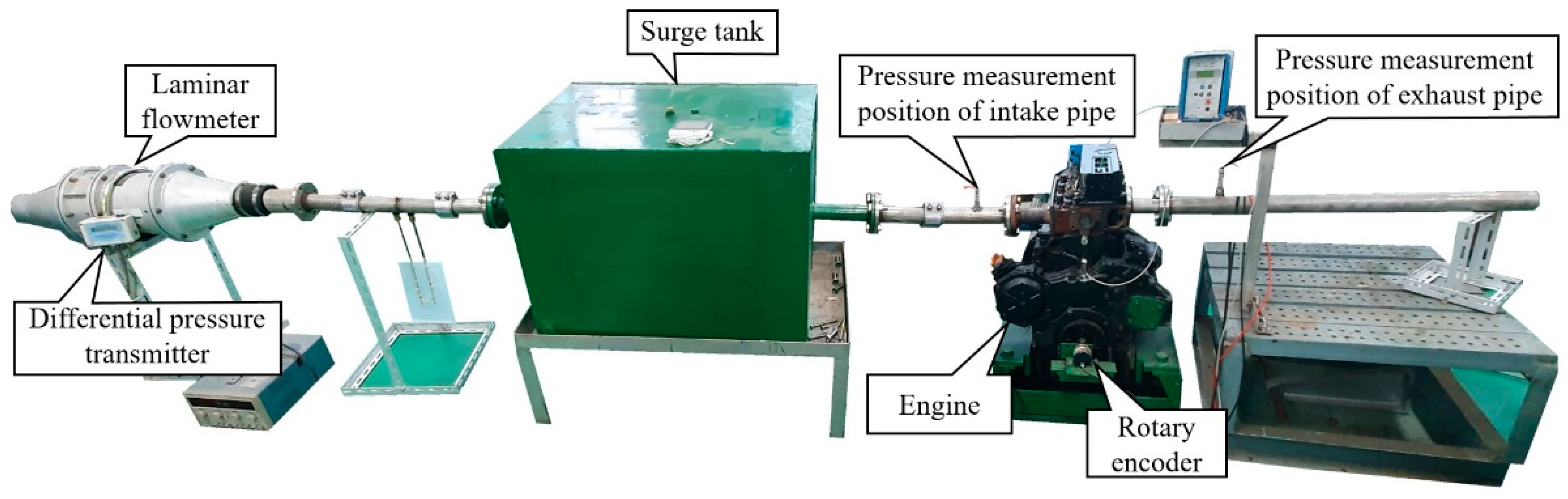
Figure 1 representing the experimental apparatus. The engine was a 35 kW three-cylinder direct injection four-stroke diesel engine. Intake and exhaust pipes were installed only in the No.1 cylinder to measure the intake and exhaust pipe pressure of a single cylinder. To observe the intake and exhaust gas flow in a cold flow state where no combustion reaction occurred, an electric motor was connected to a fly wheel in order to rotate. The mass flow rate was measured by installing a laminar flowmeter (LFE-100B, Tsukasa Sokken, Tokyo, Japan) at the starting point of the intake pipe, and the differential pressure of the laminar flowmeter was measured using a differential pressure transmitter (FCO332, Furness Controls, Bexhill-on-Sea, England) [19].
Table 1 provides the specifications of the experimental apparatus. The intake air method was in a naturally aspirated state, and the experimental data were measured at intervals of 200 rpm in the range of 700–1500 rpm of engine speed. The intake pipe from the surge tank to the cylinder head was a straight pipe with a diameter of 0.04 m and a length of 0.5 m. The exhaust pipe was a straight pipe with a diameter of 0.04 m and a length of 1.0 m, and the end of the exhaust pipe was an open-end through which the exhaust gas was released into the atmosphere. CA° refers to the crank angle degrees.
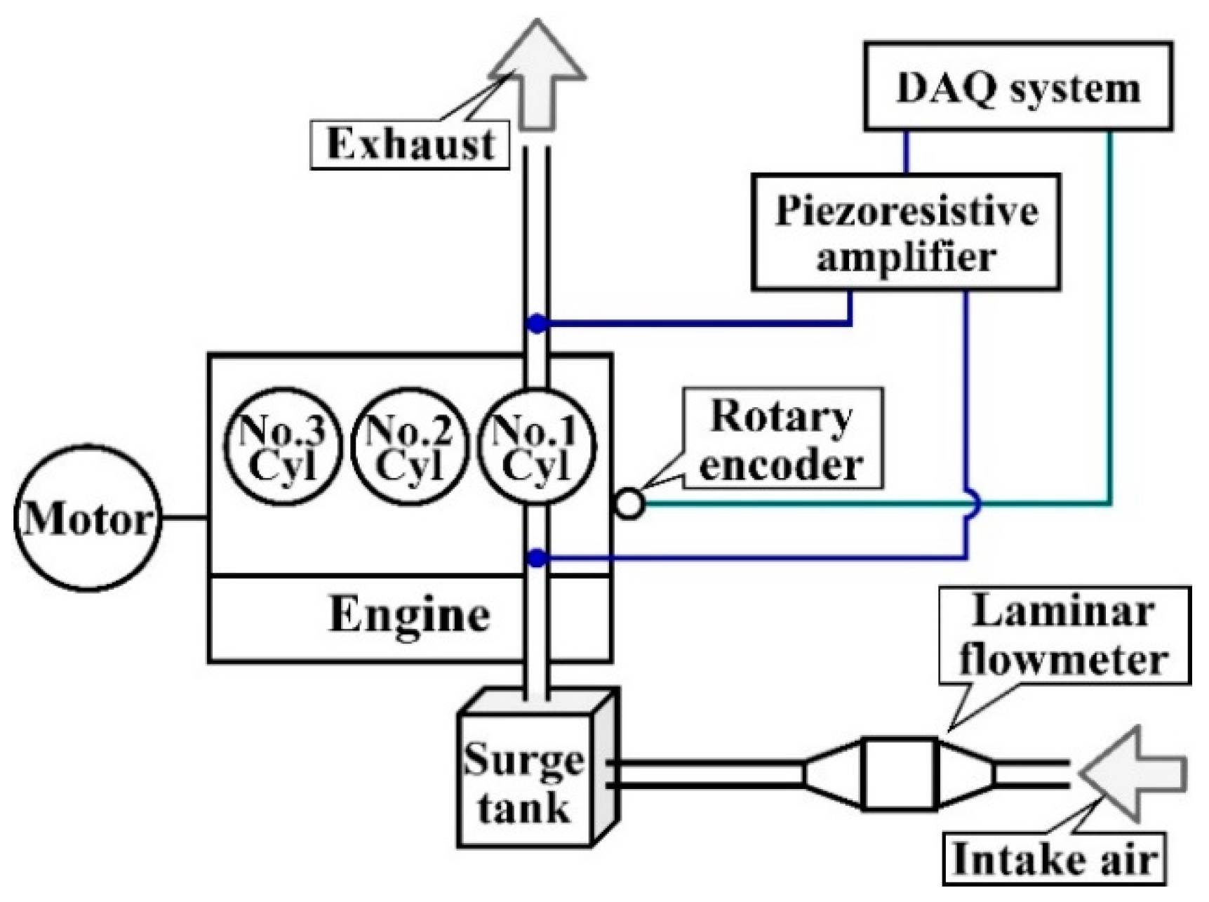
Figure 2 shows a block diagram of the experimental system. The intake and exhaust pipe pressure was measured using a data acquisition (DAQ) system consisting of a piezoresistive amplifier and a rotary encoder (E6C2-CWZ3E, Omron, Kyoto, Japan) [20]. The pressure sensors were piezoresistive (4045A5, Kistler, Winterthur, Switzerland) and the measurement point was the intake and exhaust pipe 0.15 m away from the cylinder head. The data were acquired at intervals of 0.5 CA° during 100 revolutions while the engine was stable. In order to obtain an accurate measurement, the ensemble average was applied to measured data. The ensemble average was used as a method of calculating the average of remaining values excluding the top 10% and the bottom 10% of the measured data [21]. The pressure results of the intake and exhaust pipe obtained by the ensemble average were used to verify the results of the 1D gas flow analysis.
3. Theoretical Interpretation
3.1. Average Mass Flow Rate
The equations for calculating the experimental mass flow rate to obtain the discharge coefficient is as follows. The average mass flow rate of the intake air was measured with a laminar flowmeter using Equation (1) [22].
where is the volumetric flow rate and calculated using Equation (2).
where is the laminar coefficient under standard conditions, is the viscosity depending on the air temperature, and is the differential pressure of the laminar flowmeter measured using a differential pressure meter. The average value measured during 100 revolutions for each engine speed was used, and the values are shown in Table 2.
is the density of moist air and was calculated using Equation (3).
where is the density of dry air, is the absolute humidity, and the values of each coefficient are shown in the Table 3.
3.2. Method of Charateristics
The equations for calculating the mass flow rate in 1D model to obtain the discharge coefficient is as follows.
The mass flow rate of the intake air was calculated using the MOC, as follows [18]:
where the subscript 2 refers to the downstream conditions.
The air density can be calculated with equation related to pressure, specific heat ratio and speed of sound. is the air density under downstream conditions and was calculated using Equation (5).
where subscript 01 refers to the upstream stagnation conditions.
The speed of sound was calculated using the energy equation.
Using Equations (5) and (6), Equation (4) can be expressed as follows:
to obtain the characteristics, nondimensional form is required:
Equation (8) can be computed directly from the pressure ratio across the valve or port depending on the direction of flow. When the flow is choked in the throat, Equation (8) becomes:
where subscript 0 refers to the stagnation conditions.
4. One-Dimensional Gas Flow Analysis
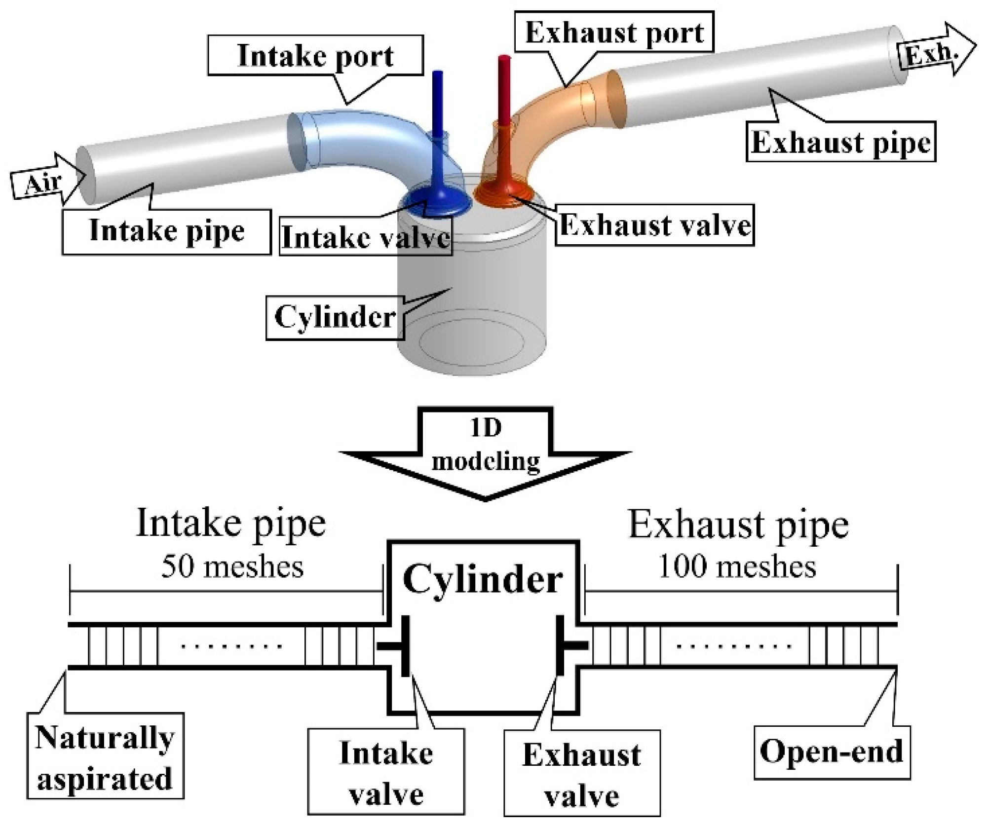
Figure 3 shows the 1D modeling of the gas flow analysis of a single cylinder diesel engine. The intake and exhaust ports are bent pipes and cannot be modeled in 1D [18,25]. Therefore, the geometry of the intake and exhaust ports was excluded from the modeling, and the length of the intake and exhaust ports was included in the intake and exhaust pipes. The only difference between the experimental and 1D modeling is the intake and exhaust ports. The purpose is to observe the errors caused by such differences, and all other boundary conditions were modeled in the same as in the experiment.
The number of meshes was 50 meshes in the intake pipe and 100 meshes in the exhaust pipe. Benson et al. verified the mesh independence in more than 12 meshes of the exhaust pipe [18], and this study confirmed the mesh independence in more than 15 meshes.
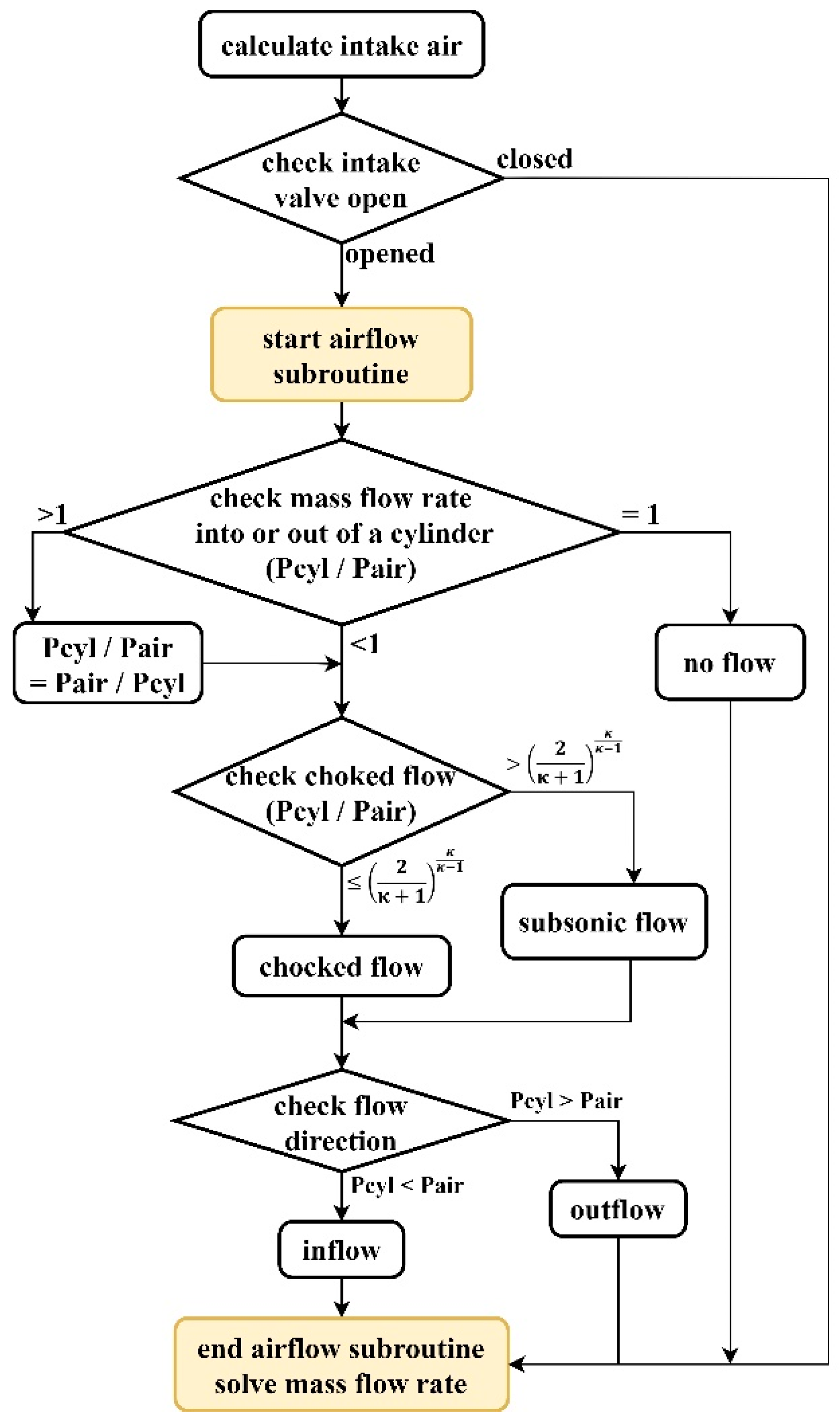
The 1D gas flow analysis of a single cylinder diesel engine was programmed using the C language. The structure of the program consisted of a main program for applying the initial conditions and calculating the pressure, velocity, and time, and a subroutine function for calculating the cylinder and intake and the exhaust gas flow [18]. Figure 4 shows the algorithm for calculating the intake air mass flow rate among the subroutine functions.
The calculation of the intake subroutine function came after the cylinder subroutine function, which calculated the pressure and mass flow rate of the cylinder. If the intake valve was open, the intake subroutine function was started. Through the cylinder pressure and intake pressure ratio, it was possible to determine the choked flow, and to calculate whether the type of flow from the cylinder was inflow or outflow. When the characteristics of the flow are determined through the calculation algorithm, the mass flow rate can be calculated using Equation (8) or Equation (9).
5. Results
5.1. Average Mass Flow Rate and Discharge Coefficient
The discharge coefficient was used to correct the difference between the 1D gas flow analysis and the measurement results. The reason is to use the gas flow analysis results to predict the performance of the experimental apparatus.
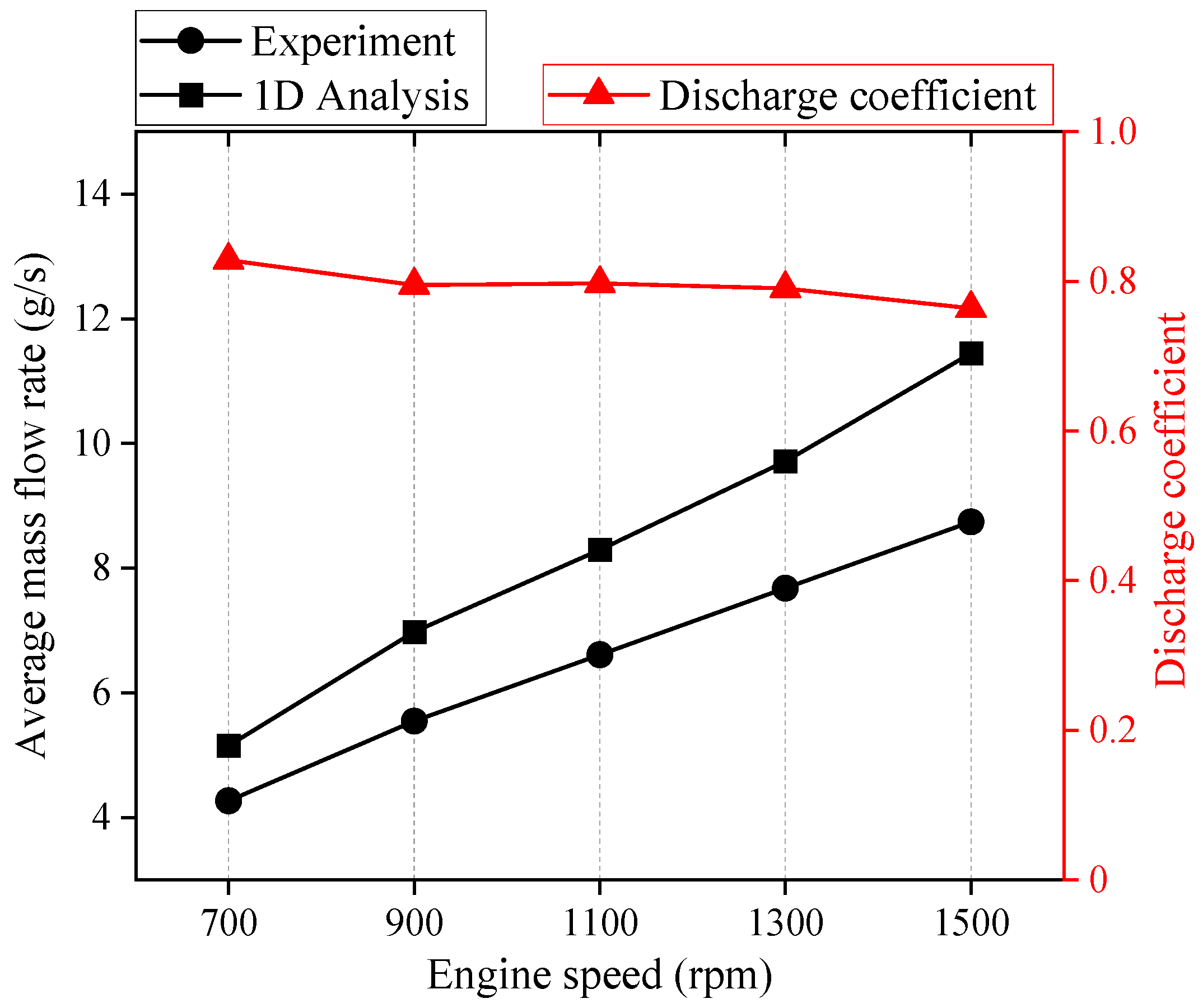
Figure 5 and Table 4 show the average mass flow rate and the discharge coefficient of the intake air according to the engine speed.
The experimental results refer to the average mass flow rate measured using a laminar flowmeter. In order to compare the average mass flow rate, the mass flow rate calculation results of the 1D gas flow rate analysis were converted to the average mass flow rate [26].
The volumetric efficiency associated with the average mass flow rate did not continue to increase in proportion to the engine speed due to valve overlap, the influence of the reflected waves, etc. However, in terms of the engine of this study, it was confirmed through a previous study that the volumetric efficiency increases in proportion to the engine speed up to 1700 rpm [22]. As the engine speed increased to 1500 rpm, the average mass flow rate increased, and the difference between the experiment and the 1D flow analysis results also increased. The reason for the difference in the average mass flow rate is the difference between the actual physical phenomena and the theoretical calculations [27,28]. The higher engine speed is the larger flow rate into the cylinder, so the difference is thought to have occurred because of this. In order to correct the differences in the results of the 1D gas flow analysis, the discharge coefficient was calculated using Equation (10). The discharge coefficient obtained in this way is a correction method for the difference between the experiment and 1D gas flow analysis. Therefore, it can be used to predict the performance of the experimental apparatus through the results of 1D gas flow analysis in the future.
5.2. Mass Flow Rate in One-dimensional Gas Flow Analysis
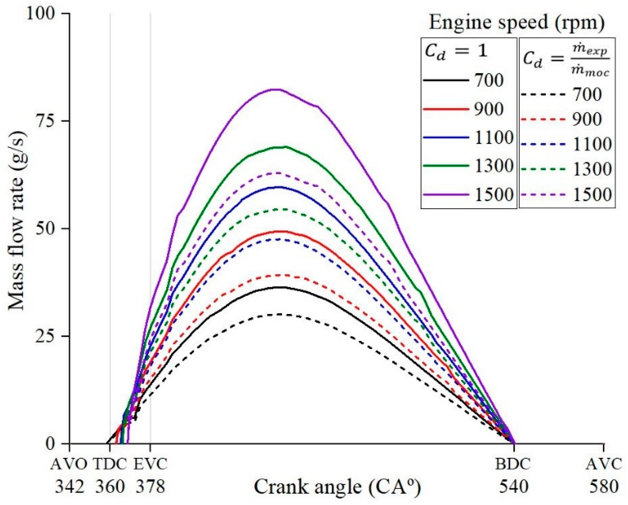
One-dimensional gas flow analysis can calculate the mass flow rate over time [18]. Figure 6 shows the intake air mass flow rate during the intake period compared to the case where the discharge coefficient was applied.
The mass flow rate does not increase as soon as the intake valve was opened [29]. This is because, during the valve overlap period (342~378 CA°), the outflow from the cylinder exits through the exhaust port. The higher engine speed is the larger gas exchange flow rate, so the timing at which the mass flow rate increases is delayed. The mass flow rate increases after the top dead center (TDC; 360 CA°), and the intake air enters the cylinder until the bottom dead center (BDC; 540 CA°). If the mass flow rate is large, the corrected value due to the application of the discharge coefficient also increases. Therefore, the correction of the result through the application of the discharge coefficient has more influence on the results of the gas exchange process in the valve open state than in the valve closed state.
5.3. Intake Pipe Pressure
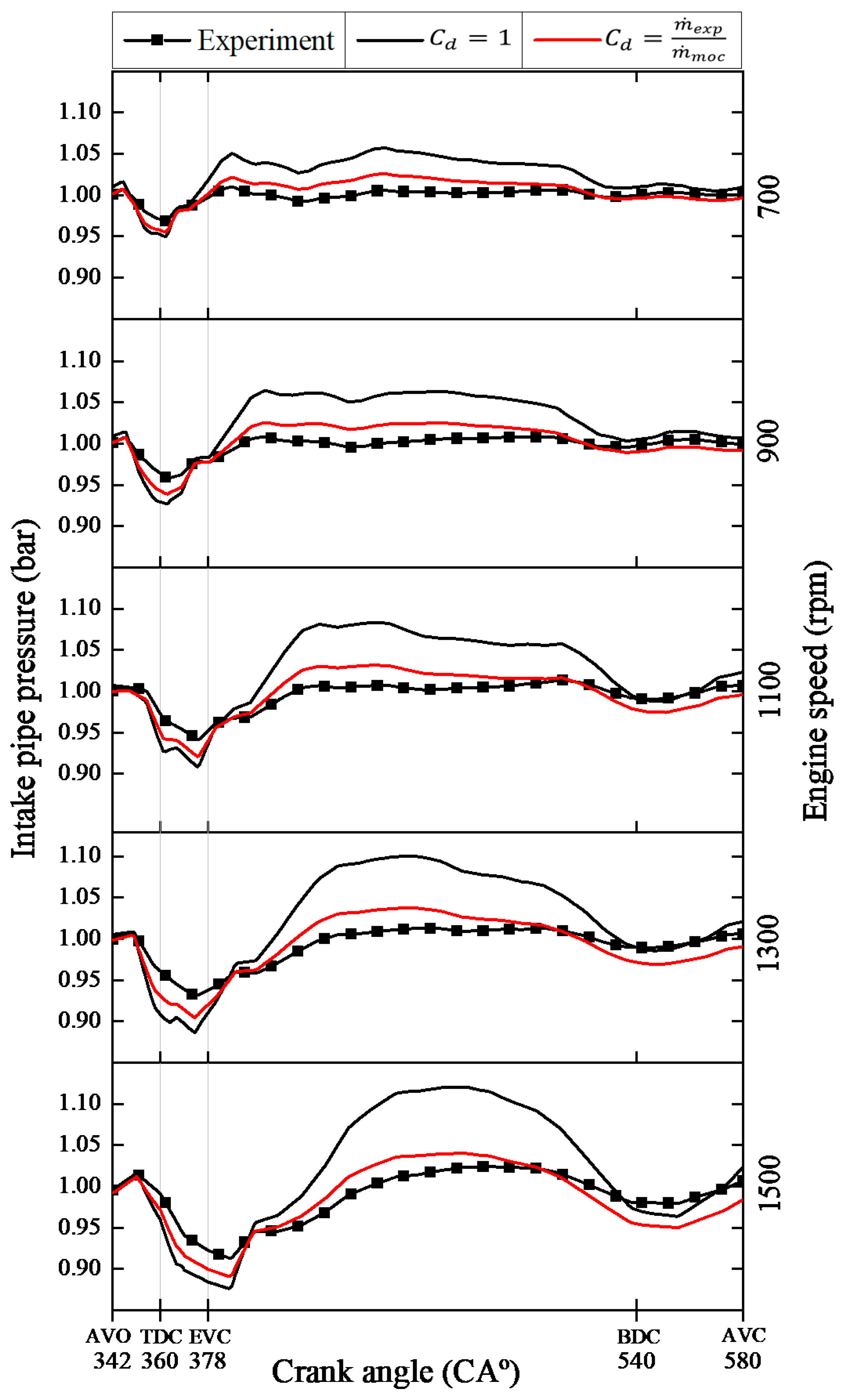
Figure 7 shows the intake pipe pressure results during the intake period. The higher engine speed is the greater negative pressure [30], and the time when the greatest negative pressure occurred was the same as in the experiment and in the 1D gas flow analysis. The phase difference occurred within 0.5 CA°.
After the exhaust valve closes (EVC; 378 CA°), there is no flow from the cylinder to the exhaust, and the flow enters the cylinder through the intake system. The time it takes for the pressure to rise to atmospheric pressure appeared later as the engine speed increased, which is thought to be due to the large flow rate that entered the cylinder.
By applying a discharge coefficient, errors within the experimental results were reduced. Even when the discharge coefficient was applied, the negative pressure and the pressure change were larger in the 1D gas flow analysis compared to the experiment [31]. The error of the maximum negative pressure decreased by 0.56–1.93% after applying the discharge coefficient and the maximum pressure error decreased by 3.11–7.86%. This is expected to be an error caused by modeling the intake and exhaust ports as straight pipes. When the piston goes down from TDC to BDC, the amount of intake is more in a straight pipe and more gas exchanged in intake and exhaust because there is less loss compared to bent pipes due to an eddy through the pipe [32,33].
In straight pipes, reflected waves are generated at the end of the pipe. However, in bent pipes, reflected waves are generated passing through the bent area [34]. The error in the 1D gas flow analysis is thought to have been caused by not calculating the influence of the reflected wave in bent pipes, as in the experiment [35]. It is expected that errors can be reduced if the geometry of bent pipes, which cannot be modeled in 1D, such as intake ports, are analyzed in 3D and are coupled [36,37].
5.4. Exhaust Pipe Pressure
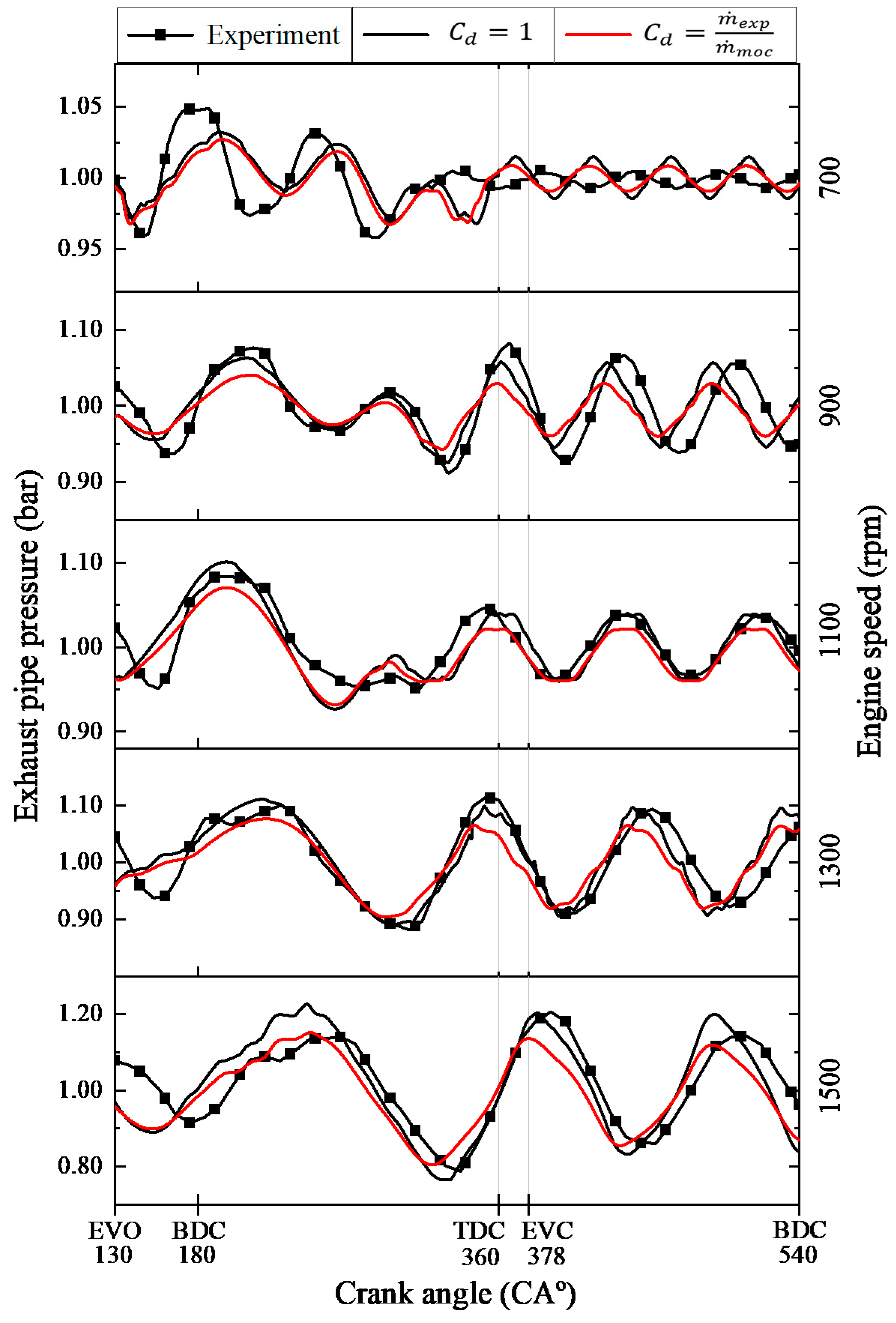
Figure 8 shows the exhaust pipe pressure results from the exhaust period to the BDC. Comparing the 1D gas flow analysis results at 700 rpm with those of the experiment, it can be seen that the amount of pressure change was small during the exhaust period (130~378 CA°). The phase difference occurred after the EVC. The reason for the phase difference is that the engine speed is slow and the reflected wave affects it many times [38]. In the case of 700 rpm, the fourth reflected wave was reached during EVC to BDC. At 900 rpm or more, the third or less reflected waves were reached. As the 1D gas flow analysis did not model the exhaust port of bent geometry, it is expected that more errors would have occurred as the influence of the reflected wave increased.
In the results above 900 rpm, the amount of pressure change was similar or large during the exhaust period. The phase difference occurred after the peak of the pressure wave appeared, which was smaller than that of 700 rpm. The peak of the pressure wave occurred due to the influence of the reflected wave [39]. In all of the results, as the influence of the reflected wave increased, a larger error occurred.
As a result of the calculation by applying the discharge coefficient, the size of the pressure change was reduced, and the phase was not affected. The reason for the phase difference likely occurred because the effect of the reflected wave generated at the open end of the exhaust pipe reached the exhaust port and affected the calculation. For the same reason as the intake port, the exhaust port could not be modeled in the same geometry as in the experiment. It is necessary to reduce the error in the 1D gas flow analysis caused by bent pipes not only for the intake system, but also for the exhaust system.
When the discharge coefficient was applied, the error of the minimum pressure increased by 0.46–6.14%. In addition, the error of the maximum pressure increased by 0.53–5.03% at 900 rpm or higher. Applying the discharge coefficient was not effective in reducing the error of the exhaust pipe pressure.
Summarizing the intake and exhaust pipe pressure results, the error of the intake pipe pressure is improved. However, since it is a result of reducing the difference in the intake mass flow rate, it is not a fundamental improvement method for the error occurring in the 1D gas flow analysis. Also, the error of the exhaust pipe pressure was not improved even when the discharge coefficient was applied. It is expected that such errors will be improved only when a method to improve errors occurring in complex shapes, which is a disadvantage of 1D, is used.
6. Conclusions
A 1D gas flow analysis was performed using the MOC for a single cylinder diesel engine, and the results of comparing the average mass flow rate and the intake and exhaust pipe pressure with the results of the experiment are summarized as follows:
- (1)
- The average mass flow rate of the 1D gas flow analysis was larger than that of the experimental results, and the discharge coefficient was calculated using this.
- (2)
- The 1D gas flow analysis was performed by applying the discharge coefficient, and the accuracy of the intake pipe pressure results was improved.
- (3)
- In the exhaust pipe result of the 1D gas flow analysis, there was a difference in pressure and phase, and there was no improvement even when the discharge coefficient was applied.
- (4)
- Applying the discharge coefficient is not a fundamental method to improve the error of 1D gas flow analysis, and the error that occurs due to the complex shape must be improved.
- (5)
- If the shortcomings of the 1D gas flow analysis, which cannot model the bent pipe geometry of the intake and exhaust ports, are compensated, the error is expected to decrease.
As a result of the experiment and verification, there was a limit to increasing the accuracy, even when applying the discharge coefficient obtained using the average mass flow rate. This error is thought to be due to the disadvantage of 1D gas flow analysis, which cannot calculate complex geometries. In the future, it is expected that this problem can be solved by analyzing the complex geometries in 3D and using 1D–3D coupling gas flow analysis.
Author Contributions
Conceptualization and methodology, K.-J.K.; experimental system configuration and data curation, K.-H.K.; software, K.-J.K.; writing and validation, K.-J.K. and K.-H.K.; supervision, K.-J.K. and K.-H.K. All authors have read and agreed to the published version of the manuscript.
Funding
This research received no external funding.
Acknowledgments
The authors would like to acknowledgment the Turbo Engine Lab, Department of Mechanical System Engineering, Pukyong National University for purchasing and supporting the use of the experimental apparatus.
Conflicts of Interest
The authors declare no conflict of interest.
References
- Abdullah, N.R.; Shahruddin, N.S.; Mamat, R.; Mohd, A.; Mamat, I.; Zulkifli, A. Effects of air intake pressure on the engine performance, fuel economy and exhaust emissions of a small gasoline engine. J. Mech. Eng. Sci. 2014, 6, 949–958. [Google Scholar] [CrossRef]
- Schulten, P.J.M.; Stapersma, D. Mean value modelling of the gas exchange of a 4-stroke diesel engine for use in powertrain applications. SAE Tech. Pap. 2003. [Google Scholar] [CrossRef]
- Kocher, L.; Koeberlein, E.; Van Alstine, D.G.; Stricker, K.; Shaver, G. Physically based volumetric efficiency model for diesel engines utilizing variable intake valve actuation. Int. J. Engine Res. 2012, 13, 169–184. [Google Scholar] [CrossRef]
- Lu, X.-C.; Yang, J.-G.; Zhang, W.-G.; Huang, Z. Effect of cetane number improver on heat release rate and emissions of high speed diesel engine fueled with ethanol–diesel blend fuel. Fuel 2004, 83, 2013–2020. [Google Scholar] [CrossRef]
- Papagiannakis, R.G.; Rakopoulos, C.D.; Hountalas, D.T.; Rakopoulos, D.C. Emission characteristics of high speed, dual fuel, compression ignition engine operating in a wide range of natural gas/diesel fuel proportions. Fuel 2010, 89, 1397–1406. [Google Scholar] [CrossRef]
- Kopac, M.; Kokturk, L. Determination of optimum speed of an internal combustion engine by exergy analysis. Int. J. Energy 2005, 2, 40–54. [Google Scholar] [CrossRef] [Green Version]
- International Maritime Organization (IMO). Effective date of implementation of the fuel oil standard in regulation. Marpol Annex VI Resolut. MEPC 2016, 280, 1. [Google Scholar]
- Johnson, B.T. Diesel Engine Emissions and Their Control. Platin. Met. Rev. 2008, 52, 23–37. [Google Scholar] [CrossRef]
- Davies, P.O.A.L. Piston engine intake and exhaust system design. J. Sound Vib. 1996, 190, 677–712. [Google Scholar] [CrossRef]
- Albarbar, A. Diesel engine fuel injection monitoring using acoustic measurements and independent component analysis. Measurement 2010, 43, 1376–1386. [Google Scholar] [CrossRef] [Green Version]
- Onorati, A.; Montenegro, G.; D’Errico, G.; Piscaglia, F. Integrated 1d–3d fluid dynamic simulation of a turbocharged diesel engine with complete intake and exhaust systems. SAE Tech. Pap. 2010. [Google Scholar] [CrossRef]
- Wurzenberger, J.C.; Wanker, R. Multi-Scale Scr Modeling, 1d Kinetic Analysis and 3d System Simulation; SAE International: Warrendale, PA, USA, 2005. [Google Scholar] [CrossRef]
- Zinner, C.; Jandl, S.; Schmidt, S. Comparison of different downsizing strategies for 2- and 3-cylinder engines by the use of 1d-cfd simulation. In Proceedings of the SAE/JSAE 2016 Small Engine Technology Conference & Exhibition, Charleston, SC, USA, 15–17 November 2016. [Google Scholar]
- Kim, K.H.; Kong, K.J. Validation of diesel engine gas flow one-dimensional numerical analysis using the method of characteristics. J. Korean Soc. Fish Ocean Technol. 2020, 56, 230–237. [Google Scholar] [CrossRef]
- Brown, G.L. Determination of two-stroke engine exhaust noise by the method of characteristics. J. Sound Vib. 1982, 82, 305–327. [Google Scholar]
- Winterbone, D.E.; Pearson, R.J. Theory of Engine Manifold Design: Wave Action Methods for IC Engines; Wiley-Blackwell: Hoboken, NJ, USA, 2000; pp. 179–274. [Google Scholar]
- Winterbone, D.E.; Pearson, R.J. Design Techniques for Engine Manifolds: Wave Action Methods for IC Engines; Wiley-Blackwell: Hoboken, NJ, USA, 1999; pp. 27–150. [Google Scholar]
- Benson, R.S.; Horlock, J.H.; Winterbone, D.E. The Thermodynamics and Gas Dynamics of Internal-Combustion Engines; Oxford University Press: Oxford, UK, 1982; Volume 1, pp. 73–313. [Google Scholar]
- Ohtsubo, H.; Yamauchi, K.; Nakazono, T.; Yamane, K.; Kawasaki, K. Influence of compression ratio on performance and variations in each cylinder of multi-cylinder natural gas engine with pcci combustion. SAE Trans. 2007, 116, 396–404. [Google Scholar]
- Han, B.; Guan, X.; Ou, J. Electrode design, measuring method and data acquisition system of carbon fiber cement paste piezoresistive sensors. Sens. Actuators A 2007, 135, 360–369. [Google Scholar] [CrossRef]
- Amann, C.A. Cylinder-pressure measurement and its use in engine research. SAE Trans. 1985, 94, 418–435. [Google Scholar]
- Lee, S.D.; Kang, H.Y.; Koh, D.K.; Ahn, S.K. The effect of intake and exhaust pulsating flow on the volumetric efficiency in a diesel engine. J. Korean Soc. Power Syst. Eng. 2006, 9, 19–25. [Google Scholar]
- Borghei, S.M.; Jalili, M.R.; Ghodsian, M. Discharge coefficient for sharp-crested side weir in subcritical flow. J. Hydraul. Eng. 1999, 125. [Google Scholar] [CrossRef]
- Chu, C.R.; Chiu, Y.-H.; Chen, Y.-J.; Wang, Y.-W.; Chou, C.-P. Turbulence effects on the discharge coefficient and mean flow rate of wind-driven cross-ventilation. Build. Environ. 2009, 44, 2064–2072. [Google Scholar] [CrossRef]
- Hufnagel, L.; Canton, J.; Örlü, R.; Marin, O.; Merzari, E.; Schlatter, P. The three-dimensional structure of swirl-switching in bent pipe flow. J. Fluid Mech. 2018, 835, 86–101. [Google Scholar] [CrossRef] [Green Version]
- Tabaczynski, R.J.; Heywood, J.B.; Keck, J.C. Time-resolved measurements of hydrocarbon mass flowrate in the exhaust of a spark-ignition engine. SAE Tech. Pap. 1972. [Google Scholar] [CrossRef]
- Ramezanizadeh, M.; Alhuyi Nazari, M.; Ahmadi, M.H.; Chau, K. Experimental and numerical analysis of a nanofluidic thermosyphon heat exchanger. Eng. Appl. Comput. Fluid Mech. 2019, 13, 40–47. [Google Scholar] [CrossRef]
- Kim, S.J.; Jang, S.P. Experimental and numerical analysis of heat transfer phenomena in a sensor tube of a mass flow controller. Int. J. Heat Mass Transf. 2001, 44, 1711–1724. [Google Scholar] [CrossRef]
- Harrison, M.F.; Stanev, P.T. Measuring wave dynamics in ic engine intake systems. J. Sound Vib. 2004, 269, 389–408. [Google Scholar] [CrossRef] [Green Version]
- Ceccarani, M.; Rebottini, C.; Bettini, R. Engine misfire monitoring for a v12 engine by exhaust pressure analysis. SAE Tech. Pap. 1998. [Google Scholar] [CrossRef]
- Takahashi, H.; Ogino, S.; Nishimura, T.; Okuno, Y. Experimental analysis for the improvement of radiator cooling air intake and discharge. SAE Tech. Pap. 1992. [Google Scholar] [CrossRef]
- Lu, J.-T.; Hsueh, Y.-C.; Huang, Y.-R.; Hwang, Y.-J.; Sun, C.-K. Bending loss of terahertz pipe waveguides. Opt. Express 2010, 18, 26332–26338. [Google Scholar] [CrossRef]
- Simizu, Y.; Sugino, K.; Kuzuhara, S. Hydraulic losses and flow patterns in bent pipes. Bull. JSME 1982, 25, 24–31. [Google Scholar] [CrossRef] [Green Version]
- Ohyagi, S.; Obara, T.; Nakata, F.; Hoshi, S. A numerical simulation of reflection processes of a detonation wave on a wedge. Shock Waves 2000, 10, 185–190. [Google Scholar] [CrossRef]
- Parker, K.H.; Jones, C.J.H. Forward and Backward Running Waves in the Arteries: Analysis Using the Method of Characteristics. J. Biomech. Eng. 1990, 112, 322–326. [Google Scholar] [CrossRef]
- Kong, K.-J.; Jung, S.-H.; Jeong, T.-Y.; Koh, D.-K. 1d–3d coupling algorithm for unsteady gas flow analysis in pipe systems. J. Mech. Sci. Technol. 2019, 33, 4521–4528. [Google Scholar] [CrossRef]
- Coghe, A.; Brunello, G.; Tassi, E. Effects of Intake Ports on the In-Cylinder Air Motion under Steady Flow Conditions. SAE Tech. Pap. 1988. [Google Scholar] [CrossRef]
- HeyWood, J. Internal Combustion Engine Fundamental; McGraw-Hill Book Company: New York, NY, USA, 1988; pp. 748–8161. [Google Scholar]
- Khir, A.W.; Parker, K.H. Measurements of wave speed and reflected waves in elastic tubes and bifurcations. J. Biomech. 2002, 35, 775–783. [Google Scholar] [CrossRef]
Figure 1.
Photograph of the experimental apparatus.

Figure 2.
Block diagram of the experimental system. DAQ: data acquisition.

Figure 3.
One-dimensional (1D) modeling of the gas flow analysis of a single cylinder diesel engine.
Figure 3.
One-dimensional (1D) modeling of the gas flow analysis of a single cylinder diesel engine.

Figure 4.
Algorithm for calculating the intake mass flow rate of the one-dimensional gas flow analysis program.
Figure 4.
Algorithm for calculating the intake mass flow rate of the one-dimensional gas flow analysis program.

Figure 5.
Average mass flow rate and discharge coefficient of intake air.

Figure 6.
One-dimensional analysis results of the mass flow rate. AVC, air–intake valve closes; AVO, air–intake valve opens; BDC, bottom dead center; EVC, exhaust valve closes; TDC, top dead center.
Figure 6.
One-dimensional analysis results of the mass flow rate. AVC, air–intake valve closes; AVO, air–intake valve opens; BDC, bottom dead center; EVC, exhaust valve closes; TDC, top dead center.

Figure 7.
Comparison of the experiment and 1D gas flow analysis results of the intake pipe pressure during the intake period.
Figure 7.
Comparison of the experiment and 1D gas flow analysis results of the intake pipe pressure during the intake period.

Figure 8.
Comparison of the experiment and 1D gas flow analysis results of the exhaust pipe pressure during the exhaust period to the BDC.
Figure 8.
Comparison of the experiment and 1D gas flow analysis results of the exhaust pipe pressure during the exhaust period to the BDC.


Table 1.
Specifications of the experimental apparatus.
| Parameter | Value | Unit |
|---|---|---|
| Engine speed | 700, 900, 1100, 1300, 1500 | rpm |
| Cylinder bore × stroke | 0.10 × 0.11 | m |
| Compression ratio | 17.6 | - |
| Intake air method | Naturally aspirated | - |
| Volume of intake port | 94.25 | cm³ |
| Length of exhaust pipe | 0.5 | m |
| Diameter of exhaust pipe | 0.04 | m |
| Air–intake valve opens (AVO) | 342 | CA° |
| Air–intake valve closes (AVC) | 580 | CA° |
| Volume of exhaust port | 32.96 | cm³ |
| Length of exhaust pipe | 1.0 | m |
| Diameter of exhaust pipe | 0.04 | m |
| Exhaust valve opens (EVO) | 130 | CA° |
| Exhaust valve closes (EVC) | 378 | CA° |
Table 2.
Differential pressure according to the engine speed.
| Engine Speed (rpm) | Px (mmH2O) |
|---|---|
| 700 | 2.0 |
| 900 | 2.6 |
| 1100 | 3.1 |
| 1300 | 3.6 |
| 1500 | 4.1 |
Table 3.
Values of coefficients.
| Coefficient | Value |
|---|---|
| ( | |
| ( | 1.2250 |
| (kg/kg) | 0.01062 |
Table 4.
Comparison of the average mass flow rate and the discharge coefficient according to the engine speed.
Table 4.
Comparison of the average mass flow rate and the discharge coefficient according to the engine speed.
| Engine Speed (rpm) | Average Mass Flow Rate (g/s) | Discharge Coefficient | |
|---|---|---|---|
| Experiment | 1D Analysis | ||
| 700 | 4.2684 | 5.1533 | 0.8283 |
| 900 | 5.5480 | 6.9780 | 0.7951 |
| 1100 | 6.6140 | 8.2969 | 0.7972 |
| 1300 | 7.6797 | 9.7150 | 0.7905 |
| 1500 | 8.7451 | 11.4471 | 0.7640 |
Publisher’s Note: MDPI stays neutral with regard to jurisdictional claims in published maps and institutional affiliations. |
© 2020 by the authors. Licensee MDPI, Basel, Switzerland. This article is an open access article distributed under the terms and conditions of the Creative Commons Attribution (CC BY) license (http://creativecommons.org/licenses/by/4.0/).
Share and Cite
MDPI and ACS Style
Kim, K.-H.; Kong, K.-J. One-Dimensional Gas Flow Analysis of the Intake and Exhaust System of a Single Cylinder Diesel Engine. J. Mar. Sci. Eng. 2020, 8, 1036. https://doi.org/10.3390/jmse8121036
AMA Style
Kim K-H, Kong K-J. One-Dimensional Gas Flow Analysis of the Intake and Exhaust System of a Single Cylinder Diesel Engine. Journal of Marine Science and Engineering. 2020; 8(12):1036. https://doi.org/10.3390/jmse8121036
Chicago/Turabian StyleKim, Kyong-Hyon, and Kyeong-Ju Kong. 2020. "One-Dimensional Gas Flow Analysis of the Intake and Exhaust System of a Single Cylinder Diesel Engine" Journal of Marine Science and Engineering 8, no. 12: 1036. https://doi.org/10.3390/jmse8121036
Note that from the first issue of 2016, this journal uses article numbers instead of page numbers. See further details here.