Tsunami Damage Detection with Remote Sensing: A Review


1
International Research Institute of Disaster Science, Tohoku University, Sendai 980-8572, Japan
2
Japan-Peru Center for Earthquake Engineering Research and Disaster Mitigation, National University of Engineering, Lima 15333, Peru
3
Center for Applied Statistics, School of Statistics, Renmin University of China, Beijing 100872, China
*
Author to whom correspondence should be addressed.
†
Current address: International Research Institute of Disaster Science, Tohoku University, Aoba 468-1, Aramaki, Aoba-ku, Sendai 980-8572, Japan.
Geosciences 2020, 10(5), 177; https://doi.org/10.3390/geosciences10050177
Submission received: 17 April 2020
/
Accepted: 30 April 2020
/
Published: 12 May 2020
(This article belongs to the Special Issue Remote Sensing Application for Earthquake and Tsunami Damage Assessment)
Abstract
:Tsunamis are rare events compared with the other natural disasters, but once it happens, it can be extremely devastating to the coastal communities. Extensive inland penetration of tsunamis may cause the difficulties of understanding its impact in the aftermath of its generation. Therefore the social needs to technologies of detecting the wide impact of great tsunamis have been increased. Recent advances of remote sensing and technologies of image analysis meet the above needs and lead to more rapid and efficient understanding of tsunami affected areas. This paper provides a review of how remote sensing methods have developed to contribute to post-tsunami disaster response. The evaluations in the performances of the remote sensing methods are discussed according to the needs of tsunami disaster response with future perspective.
1. Introduction
The word Tsunami comes from a Japanese term derived from the characters “tsu” (meaning harbor) and “nami” (meaning wave), and is now widely common in the world. Physically, tsunami is defined as a series of water waves caused by the sudden displacement of a large volume of water, usually in the sea or even in a large lake. Tremendous volumes of water displacement makes a tsunami and devastate coastal regions, sometimes across the ocean. Earthquakes, volcanic eruptions, landslides, underwater landslides, and large mass impact into the ocean (meteorite/asteroid impacts or similar impact events) all have potentials to generate tsunamis.
Tsunami events are rare compared with the other natural disasters but can be extremely devastating. In total, 16 major tsunamis killed 250,900 people in 21 countries between 1996 and 2015 [1,2], and it averages more than 15,600 deaths per single event. This rate is likely to be high compared with other natural disasters including storms (such as cyclones or typhoons), floods, and earthquakes. It is also true that this rate is significantly contributed by two catastrophic events; the 2004 Sumatra–Andaman earthquake tsunami (hereafter, Indian Ocean tsunami) and the 2011 Great East Japan earthquake tsunami (hereafter, Tohoku tsunami), but it characterizes a tsunami as a devastating natural disaster [3].
In the aftermath of catastrophic tsunami disasters, our society is confronted with significant difficulties of understanding impacts with the limited time, resources, and information. For instance, in the 2004 Indian Ocean tsunami that propagated the entire Indian Ocean and caused extensive impacts to 12 countries. As a result of the vast damage on structures, infrastructures, communication networks, and the failure of emergency response system, whole picture of the impact could not be addressed for months.
Thanks to recent advances and improvements in satellite sensors, data accessibility, applications, and services, many space agencies support data-sharing policies that facilitate access to remotely-sensed data for more efficient use in disaster management [4]. Tremendous progress has been made with sophisticated methods to analyze imageries and geospatial data in near real-time via geo-web-services and crowd-sourcing [5], and those can be used in disaster management and emergency response. Satellite earth observations achieved consistent and repeated coverage of the world, and that makes it possible to understand and share the information on disaster impacts among the countries, regardless of time and weather conditions.
This paper aims to provide a review of the advances of remote sensing methods and its applications to detecting the tsunami impacts, and to evaluate their performances in post-disaster response point of view with some discussions of future perspective. The paper is organized as follows. Section 2 describes the physical characteristics of tsunamis and summarizes the features that can be acquired by remote sensing. Section 3 focuses on the consequences of tsunami’s inland penetration and discusses the tsunami damage interpretation by various sensors and platforms. Section 4 and Section 5 introduce recent advances of machine/deep learning to detect tsunami damage and discusses its performances. Section 6 discusses future perspectives of machine/deep learning to enhance tsunami damage detection capability. Section 7 presents our conclusions.
2. Tsunami Physics and Acquisition of Tsunami Features with Remote Sensing
What tsunami features can be acquired by remote sensing platforms and sensors during its generation, propagation and after inland penetration? This is an interesting question, since tsunamis are unpredictable phenomena. Table 1 summarizes the remote sensing platforms and sensors that have acquired tsunami features during and after the events.
Tsunami is categorized as long wave in water surface waves, and its wave length is much longer than the water depth where a tsunami propagates [3]. In general, when , a wave has the characteristics of long wave. Consider a tsunami is generated offshore at depths of several thousand meters by a sudden sea bottom deformation due to an earthquake. The wavelength of a traveling tsunami varies from tens to hundreds of kilometers according to the fault rupture scale and the sea surface height varies from several centimeters to several meters. In many cases, tsunamis in such deep water are much smaller in amplitude than those near the coasts, then are amplified enormously as approaching the coasts. This makes tsunamis difficult to detect over deep water, where ships are unable to feel their passage, and it has been believed that only some offshore sensors, e.g., ocean bottom pressure sensors [6], can detect the tsunami’s passage.
However, there was probably only an exception in 2004. The tsunami passage in the Indian Ocean, generated by the 2004 Sumatra–Andaman earthquake, was measured by Jason–1 satellite. Jason–1 was a mission satellite launched by National Aeronautics and Space Administration (NASA, United States) and Centre National d’études Spatiales (CNES, France) and has measured the sea surface height of traveling tsunami along the track approximately two hours after the earthquake. This was probably the first example for satellite remote sensing to detect the traveling tsunami in mid–ocean [7]. Figure 1 illustrates the track of Jason–1 (track 109) on 26 December 2004 and the extracted tsunami height along the track [8]. In the figure, the snapshot of modeled tsunami at 2 h after the earthquake is shown to explain how Jason–1 measured the sea surface height along tsunami propagation direction. Jason–1 clearly detected the sea surface of tsunami front and its peak propagating southward from S to S in latitude, which is critical to determine the tsunami source model [9], i.e., tsunami generation mechanism.
As a tsunami approaches the coast and the water depth becomes shallower, reducing the tsunami’s traveling speed compresses the tsunami’s wave length, and its amplitude increases enormously. When a tsunami penetrates on land, its characteristic changes significantly, from that of a water wave to a strong inundation flow [3].
To describe the overland flow of a tsunami, there are some important quantities that can be measured with remote sensing, e.g., tsunami inundation extent (how far tsunami penetrates inland) and flow velocities. The aerial videos can help with understanding how the tsunami would penetrate inland. Immediately after the 2011 Tohoku tsunami occurred, NHK (Japan Broadcasting Corporation) sent a crew to Sendai coast on a helicopter to broadcast the tsunami attack. The tsunami attacked Sendai coast approximately 1 h after the earthquake and NHK crew succeeded to shoot the moment of tsunami inundation on the Sendai coast (e.g., https://www.youtube.com/watch?v=zxm050h0k2I). The video includes scientific information of the process of tsunami’s inland penetration. Figure 2 shows the procedure for mapping tsunami front [10]. The continuously recorded video was divided into individual frames to be calibrated and rectified by 2-D projective transformation with ground control points which could be identified in pre-event maps and images.
As shown in Figure 2c, the time series of tsunami front on land could be identified with the timestamps of the video. When the distance between two tsunami front lines is divided by the time between the frames, the “tsunami front velocity” can be estimated. In addition, when we focus on the movement of floating objects in the video, the “tsunami flow velocity” is measured [11]. This information is significantly valuable to understand the physical process of tsunami inland penetration, e.g., tsunami flow velocity, hydrodynamic forces on structures.
3. Tsunami Damage Interpretation in Remote Sensing
Identifying tsunami-induced building damage have been conducted in recent years with increasing interest as a response by scientists due to the devastating events and the need for rapid damage assessment to support disaster relief efforts. This section summarizes the methodologies for detecting tsunami impacts and its effects in the built-up areas recognizable as tsunami damage. Table 2 presents a list of events and related literature focusing on the tsunami-induced damage.
While remote sensing has been applied to monitoring and understanding physical processes of tsunami hazards, the impacts to the societies and damage caused by disasters need to be addressed for disaster response [12,13]. In this sense, satellite remote sensing is advantageous when the impact is of large-scale and a wide area is needed to be grasped rapidly [14]. Satellite data acquisition and fast data processing has increased through these years due to technological advances in the constellation of satellites and the interest in archiving and sharing the information gathered by multiple sensors. Thus, remote sensing has been used to estimate possible damage after major disasters [15,16].
A comprehensive review of earthquake-induced building damage detection with remote sensing was provided by past studies [17]. For instance, two approaches were discussed; multi-temporal techniques and mono-temporal techniques. A multi-temporal technique uses a pre- and post-event image to evaluate the changes between images and interpret them as possible damage. A mono-temporal method applies only post-event data. In the case of building damage induced by a tsunami, its characteristics are different from the damage mechanisms due to earthquake, therefore, some techniques follow similar principles but need further treatment to adequately interpret the level of tsunami damage [18].
First, it is important to recognize that most of the methods used for damage interpretation or damage recognition need urban-based maps (i.e., building footprint data). Sometimes also building height is required to conduct damage estimation [19,20]. Official cadastral information, open data sources (e.g., OpenStreetMap), reference sources (e.g., Google Street Map, Google Earth), and built-up area extraction methods [21,22] are used to overcome this first step in the damage assessment and damage estimation process. Otherwise, land cover classification, performed from remote sensing data collected before the disaster in question, would be necessary.
In the case of tsunami damage estimation, aerial photos [23], and optical satellite images were used first to classify tsunami affected-areas and extract inundation areas [24]. Similarly, visual interpretation of pre- and post-images of high-resolution optical images are used to classify building damage in the aftermath of a disaster [25]. Currently, this method is still conducted after many types of disasters, including meteorological hazards, geophysical hazards, deliberate and accidental man-made disasters, and other humanitarian disasters as rapid mapping efforts by emergency operational frameworks (e.g., Copernicus Emergency Management Service - European Commission [26], the UN-SPIDER [27], and the Sentinel Asia initiative in the Asia-Pacific [28]).
3.1. Extracting Tsunami Inundation Zone
3.1.1. Using Optical Images
A unique feature of tsunami inundation zone is caused by the sea water penetration on land and cascading effects. Thus, the optical satellite remote sensing for mapping tsunami affected areas focuses on extracting the changes in spectral features related to vegetation, soil, and water observed in a pair of optical satellite images.
Changes in the normalized difference vegetation index (NDVI), soil index (NDSI), and water index (NDWI) are used to extract the inundated areas. In particular case of NDWI, many uses of the spectral bands are verified when looking for land surface changes in particular water body, water level or flooding [15,24,57,58,59,60]. The use of these indices require a careful comparison of their indices between the pre- and post-event images (or between affected and non affected areas) to decide a threshold of classification. The value of this threshold maximizes the difference between cumulative frequency distributions in order to define at least two classes [24]. Theoretically, NDWI varies from to 1 according to the spectral features of ground surface. Especially, water strongly absorbs near-infrared (NIR) band of light and it indicates higher value of NDWI. Therefore, the analysis for extracting tsunami inundation is performed on the assumption that the NDWI values in the inundated areas are higher because of the existence of water, and they suddenly decrease on the dry land across the inundation limit. This is the basic idea to determine the threshold value of NDWI to extract the inundated zones.
Figure 3 shows an example of the extraction of the tsunami inundation zone after the 2011 Tohoku tsunami using ALOS/AVNIR-2 image. ALOS of Japan Aerospace eXploration Agency (JAXA) captured whole part of Sendai plain, approximately 500 from Sendai city to the south of Yamamoto town, Miyagi Prefecture. JAXA released a set of pre and post-event image of AVNIR-2 sensor immediately after the acquisition, 14 March 2011. This image significantly contributed on quick understanding of the tsunami inundation extent [10,61].
Visual inspection of the optical images in affected areas has also been studied with Digital Elevation Model (DEM) to determine tsunami run-up heights [16,62], however it might overestimate the heights due to limited resolution and accuracy of DEM used. In addition, in other areas, tsunami run-up might have been higher than interpreted through visual inspection, because the water limit was not visible due to the lack of debris or other hints of tsunami inundation. An example of inundation limit extraction using Advanced Spaceborne Thermal Emission and Reflection Radiometer (ASTER) data and Shuttle Radar Topography Mission (SRTM) data is shown in Figure 4.
3.1.2. Using Synthetic Aperture Radar (SAR) Data
Since microwaves can penetrate through clouds and can operate in day or night conditions, Synthetic Aperture Radar (SAR) is widely used for monitoring the earth surfaces. The advantage of using SAR data is well-known for detecting surface changes and displacement [63], and has been recognized to be useful for post-disaster damage assessment [30]. Since the first launch of high-resolution SAR satellites in 2007, i.e., TerraSAR-X and CosmoSkyMed, archives of high-resolution SAR data have been constructed, and these data are promising for improving the methods in damage detection.
Lower sigma naught values (strength of the reflected signal, i.e., backscattering coefficient) in SAR data indicate the areas are covered by water due to the specular reflection mechanism of the microwaves on smooth surface. Other backscattering mechanisms, such as double bounce in urban areas and volumetric scattering in forest areas, might be present as well. However, the effect of the acquisition conditions (i.e., sensor depression angle and ascending/descending satellite path) must be taken into account. Radar shadowing, layover and foreshortening are such examples. Semi-automated methods to extract tsunami inundation zone were developed using change detection in SAR data similar to optical image approaches [44,64]. Backscattering coefficients from water body and land cover areas are sampled from pre-event data. Next, a threshold value of back scattering intensity histograms is chosen so water bodies and other features can be classified reliably. Figure 5 shows an example of tsunami inundation areas extracted from TerraSAR-X images in the case of the 2011 Tohoku tsunami [64].
3.2. Interpretation of Tsunami-Induced Building Damage
Building damage interpretation is a part of the damage assessment and emergency mapping processes conducted immediately after a disaster. Several satellite-based emergency mapping (SEM) systems have been deployed by local, national and international agencies to carry out this task [65,66]. Mapping the damage helps improving disaster relief effectiveness and reduce suffering and fatalities. The Copernicus Programme [26], the UN-SPIDER [27], and the Sentinel Asia initiative in the Asia-Pacific [28] are some of the earth observation systems supporting disaster response using remote sensing technology.
To identify tsunami-induced building damage one can use optical pre- and post-event images to visually inspect the affected area and observe changes in buildings. It is also used in earthquake-induced [17] or hurricane-induced damage assessments [25,67]. Unfortunately optical images require free cloud conditions to clearly observe the earth surface. To overcome the limitation of these passive sensors (optical image), active sensors (radar satellite image) are used to identify built-up-areas [68,69] and building damage [43,70,71].
3.2.1. Using Optical Images
High-resolution satellite images and aerial photos can be used to detect individual building damage. For instance, post-tsunami satellite imagery of IKONOS was used by the Japan International Cooperation Agency (JICA) after the 2004 Indian Ocean tsunami to visually inspect the damage in Banda Aceh of Sumatra island, Indonesia [72]. This information was then used to develop tsunami fragility functions [9] as a measure to estimate the structural damage due to tsunami attack.
In case of the 2011 Tohoku tsunami, visual inspection of building damage was conducted [23] using aerial photos acquired on the following days (12, 13, 19 March and 1, 5 April of 2011) by Geospatial Information Authority of Japan (GSI). In this case, the missing roof was the proxy of classification as “washed-away” or “surviving”. While the accuracy of this method depends on quality of the image and the expert/user having a keen eye to spot changes, the time-consuming task becomes a drawback in disaster response stages (see Figure 6). Optical images would also be applied to monitor the recovery and reconstruction process after a disaster [32,33].
In addition, the use of Unmanned Aerial Vehicles (UAV) are becoming popular to obtain high-resolution images from the disaster areas. Despite its limited coverage compared to satellite images, it offers fast deployment and multiple angle footage providing valuable information for 3D mapping and higher accuracy on damage assessment for localized areas [73,74,75].
3.2.2. Using LiDAR data
Applications of Light Detection And Ranging (LiDAR) for damage detection are still few compared with other remote-sensing technologies. The main reason is the lack of LiDAR data before a disaster. Some attempts exist to monitor the tsunami affected areas focusing on accumulation of debris generated by the tsunami inundation by three dimensional mapping [42]. The authors proposed a fusion of feature extraction [40] with optical sensor data (aerial photos, satellite images) and volumetric estimation with LiDAR data. An object-based analysis of optical sensor data was used to classify/extract the debris area in the earth surface, while a digital surface model (DSM) of LiDAR data was used to estimate the volume of such debris to be used as the observation of debris removal efforts [76]. Figure 7 shows three-dimensional mapping of debris performed by integration of optical image analysis to extract tsunami debris area with the height information of objects on the ground obtained from LiDAR analysis.
A similar approach using LiDAR data can be used to estimate building damage, an example from earthquake-induced building damage can be found [77]. An example of building damage interpretation using LiDAR data is shown in Figure 8. Collapsed buildings were detected using a pair of digital surface models (DSMs), taken before and after the main shock by airborne LiDAR flights. The change in average elevation within a building footprint was found to be the most important factor.
3.2.3. Using Synthetic Aperture Radar (SAR) Data
The radar signal is primarily sensitive to surface structure. Figure 9 shows considerable patterns of land surfaces in tsunami affected area [46]. Change of signal properties in the radar data would be used to detect and evaluate the building damage. Man-made structures reveal high backscattering, i.e., high sigma naught values in the SAR data, because of double bounce, and completely washed-away or collapsed structures indicate lower backscattering. It is inferred that the change ratio in areas with high backscattering varies as washed-away or structurally destroyed. Several exceptions may be expected to characterize tsunami damage. For instance, the case shown in Figure 9B, high backscattering in slightly-damaged buildings with surrounding tsunami debris may result in false positive errors. The cases in Figure 9D,F may not reveal changes in areas with high backscattering, since the movement of buildings and accumulation of debris induce double-bounce scattering. These damage patterns may cause false negative errors. These considerable damage patterns are utilized to discuss the reasons for errors.
A number of methods have been proposed for estimating building damage caused by tsunami disasters in recent decades [41,46,48,78]. Following the 2011 Tohoku tsunami disaster, approaches using high-resolution SAR data have been proposed to detect building damage at the building unit scale. Some new approaches were proposed to classify tsunami-induced building damage into multiple classes using pre- and post-event high-resolution radar (TerraSAR-X) data. To exploit the relationships of backscattering features in the tsunami affected areas, the methods for classifying tsunami-induced building damage into multiple classes were developed by analyzing the statistical relationship between the change ratios in areas with high backscattering and in areas with building damage. Figure 10 shows an example of building damage classification in the affected areas of the 2011 Tohoku tsunami [46]. The results provided an overall accuracy of 67.4%. It can be said that the method shows a good performance for classifying damaged buildings, but more discussion has to be done to consider if this performance is acceptable in the disaster response efforts.
3.3. From Change Detection to Machine Learning Algorithms
As described in the above sections, change detection is the basis for damage interpretation using remote sensing. Change detection determines the differences in the ground surface from images acquired at different time phases. Two kinds of change detection methods are generally applied [79]; (1) Post-classification comparison and (2) comparative analysis. In the first one, the result of classification of each image is then compared to identify changed and unchanged portions [24]. The latter, however, constructs a difference image from multiple time phases and then detects the change through analysis [80]. In both methods there is a “classification” task. High accuracy of classification is required to ensure the method gives suitable results. However, classifying objects in an image through visual inspection is impractical for rapid damage assessment due to the time consuming task. An alternative is to use real-time collaborative systems and produce classification by multiple experts at the same time. This is how some of the mapping products in the Copernicus Emergency Management System are built. This will help reduce production time, however it might incorporate bias in classifications due to the differences in expertise from different producers. Another option, to overcome previous limitations, is to automatize the whole classification process via machine learning algorithms.
Incorporated supplemental GIS information and human expert knowledge into digital image processing was performed in wetland classification [81]. They describe a two stage process: (1) training and (2) learning. The processes generate a “knowledge base” which is a set of rules that can be used by the expert to perform a final image classification.
In the next section, we will discuss how machine learning and deep learning algorithms are used to support the tsunami hazard and damage assessment.
4. Application of Machine Learning to Tsunami Damage Detection
This section summarizes the machine learning (ML) algorithms applied to identify the consequences of tsunamis attack to the coast. Here we report the type of remote sensing data used, describe the feature space, and a glimpse of the ML algorithms.
Consider a set of samples computed from remote sensing, where is an n-dimensional vector, hereafter referred as feature vector. A machine learning algorithm refers to any procedure that assigns the samples a distinctive label/class. The reported methods are divided into two groups; unsupervised machine learning and supervised machine learning. In unsupervised learning, the algorithm learns only from the data. On the other hand, a supervised learning algorithm is calibrated from a subset of samples whose correct class is known beforehand.
4.1. Unsupervised Machine Learning
4.1.1. Thresholding
Thresholding is a procedure used to segment an input image into two classes [12]. A framework is implemented to select automatically samples from which the threshold is defined [78]. Here, a one-dimensional feature vector is used. Each feature represents either a difference or a log-ratio image pixel computed from a pair of images acquired before and after a tsunami. The discriminant function can be expressed as follows;
where T is the threshold value that needs to be calibrated.
With this objective, the image is split into N subimages and sorted according to their standard deviation. It is expected to find large standard deviation in subimages that contains changed pixels. Therefore, a fraction of the subimages with the largest standard deviation are used to define T. By applying standard thresholding procedures [82,83], the method was successfully used to identify damages induced by the tsunami occurred on 26 December 2004 off the north of Sumatra Island, Indonesia. Two microwave intensity images obtained from the RADARSAT-1 satellite were used. The pre and post-event images were acquired respectively in April 1998 and January 2005. Both have the same acquisition parameters and were filtered to reduce the speckle noise. The seaside pixels were masked as a preprocessing step. Then, log-ratio between the images was computed. The image was divided into 272 subimages ( pixels each), from which only 149 were used for further analysis. A total of six subimages were used to set the threshold T, where the Kittler and Illingworth algorithm, extended to a generalized Gaussian model [83] was used.
4.1.2. K-Means Clustering
The algorithm assigns a class to a sample by the following expression;
where denotes the average samples assigned to class k, and is tuned from an iterative procedure termed as maximization step. The number of classes is defined beforehand. In summary, given any starting value, the following two steps are repeated consecutively until reach convergence. First, a sample is assigned using Equation (2). Second, re-estimate the mean as the average of samples assigned to k. Convergence is guaranteed with the maximization step algorithm.
There is an example that applied k-cluster to characterize the surface tsunami effects due to the 2011 Tohoku tsunami [53]. is composed of radiance pixels extracted from visible and near-infrared (VNIR) images from ASTER satellite. The resolution of the imagery was 15 m. Four components belonged to the bands of VNIR acquired on 24 February 2011; and the other four components to that acquired on 19 March 2011. A total of 30 different classes were set, from which 6 of them were identified as flooding debris, building damage, mud, stressed, and non stressed vegetation.
4.1.3. Expectation-Maximization (EM) Algorithm
While k-means algorithm updates under a euclidean distance criterion, the expectation- maximization algorithm updates parameters of a distribution model. Here the distribution of X is assumed to represent a mixture of distributions.
where k is the number of classes defined beforehand. denotes a class and are the mixture proportions. The distributions are defined from an iterative optimization. For instance, assuming Gaussian distributions, the calibration of their parameters is as follows;
where and denote the vector mean and variance. Further reading on EM algorithm can be found in [84,85].
The EM-algorithm is employed to evaluate the performance of features computed from fully polarimetric SAR images to identify damaged areas due to the 2011 Tohoku tsunami [86]. The images were acquired at 21 November 2010 and 8 April 2011, respectively. Three groups of polarimetric features were tested. The first group is composed of the difference of surface, double-bounce, and volume scattering computed from a decomposition method [87]. The second group of features is composed of entropy, anisotropy, and average scattering angle; all computed from an eigenvalue-eigenvector decomposition [88]. The third group includes the polarimetric orientation angle, the co-polarization coherence in the linear polarization basis and in the circular polarization basis. Positive change, negative change, and no change were set as the three classes.
4.1.4. Imagery, Hazard, and Fragility Function (IHF) Method
The authors proposed a modification of the standard logistic regression classifier within a framework that can be used automatically without the use of training data [49]. As the name suggests, the discriminant function has the form of a logistic function;
where the vector w and the value are usually calibrated from training data. A sample will be predicted as damaged if ; otherwise, it is predicted as non-damaged sample. It is pointed out that some large scale disasters, such as earthquakes and tsunamis, can be numerically modeled on near real-time [49]. Furthermore, in many cases there are available the so-called fragility functions. These are functions that provide relationship between the intensity of a hazard at an arbitrary location and the expected percentage of damage. Therefore, under such situations, the discriminant function can be calibrated from the following optimization problem;
where denotes the intensity of the disaster at the location of sample . is estimated from a numerical model of the disaster, refers to an arbitrary fragility function.
Figure 11 shows a scheme of the application of the IHF method to identify washed away buildings using TerraSAR-X images, estimation of the inundation depth map, and fragility functions as inputs. First, a pair of TerraSAR-X imagery, taken before (21 October 2010) and after (13 March 2011) the 2011 Tohoku tsunami, is used to computed two parameters for each building: an averaged difference and the correlation coefficient. These parameters were computed using the bounding box of the building footprint. Additionally, each sample building is associated with an estimation of the inundation depth () at its geolocation. With the inundation depth, the probability that a sample will be washed-away can be computed with a fragility function () [89]. Then, having the three source of information (i.e., remote sensing-based features, inundation depth, and a suitable fragility function), the IHF method can be applied. A total of samples, randomly selected but uniformly distributed with respect to their inundation depth, were used to solve Equation (6). The procedure were repeated four times. The resulting linear discriminant functions are shown in the right side of Figure 11, from which it is observed the four discriminant functions are almost the same. The complete dataset (31,262 samples) is also shown, but separated in different scatter plot according to the damage level surveyed by the Ministry of Land, Infrastructure, Transport, and Tourism (MLIT) [90]. It is clearly observed that most of the washed-away buildings are located to the left side of the discriminant function; while the buildings with different damage level are located on the other side.
4.2. Supervised Machine Learning
4.2.1. Support Vector Machine
Here, we introduce Support Vector Machine (SVM) as one of supervised learning models used for classification. The discriminant function is defined as follows;
where is a function that maps the feature space to a space belonging to a kernel, . the approach lies on mapping the feature space to the space F and then define an hyperplane that separates the classes with a maximum margin. The vector w a vector in F that is perpendicular to the referred hyperplane. denotes an offset. The parameters w and are computed from the following quadratic programming problem:
The function is usually chosen beforehand based on its associated kernel. Very often the Gaussian kernel is employed;
Using SAR data was verified to identify the damaged buildings due to the 11 March 2011 Tohoku tsunami [91]. Three TerraSAR-X datasets, one was acquired before and two were acquired after the tsunami, and two scenes of ALOS PALSAR data, acquired before and after the tsunami, were used. The field survey performed by the Ministry of Land, Infrastructure, Transport, and Tourism (MLIT) [90] was used for training and evaluation. The amount and quality of the data provided by the MLIT made the 2011 tsunami a benchmark to test different algorithms. Two types of features were used. The first group is termed multi-temporal change features of a factor that consist of averaged difference, correlation coefficient [92]. These features were computed using images acquired before and after the tsunami event. The second group of features consist of statistical features, such as mode, mean, standard deviation, minimum, and maximum values. All features were computed at a building unit resolution. Different configurations were tested to evaluate the influence of the training samples, the acquisition date, the classification scheme, and the type of microwave sensor.
Not only two-level classifier; damaged and non-damaged, multi-level classifier was explored to improve the performance of the SVM as a multi-class classifier [48]. The study focused on the 2011 tsunami as well. Two microwave intensity images acquired on 20 October 2010 and 12 March 2011 by the TerraSAR-X data were used. The images were used to compute the averaged difference and the correlation coefficient using six different window sizes: , , , , , and . Thus, a total of 12 components constitutes each vector . As training data, the MLIT survey results were rearranged, under different configurations, in three groups labeled as washed away, moderate change, and slight change. Regarding the calibration of Equation (7), the Gaussian kernel were employed, Equation (10), and the parameters and were tuned using a 10-fold cross-validation.
A novel set of features was proposed to be used for damage detection [52]. These new features were computed from the gray level co-occurrence matrix (GLCM), one of many procedures available for texture analysis. The novelty in their study is that the GLCM was constructed in a three-dimensional domain, referred as 3DGLCM. That is, stacked multi-temporal imagery. Under this configuration, it was proved the 3DGLCM tend to be a near to a diagonal matrix in non-damaged areas; whereas the non-zero components are far from the diagonal in damaged areas (Figure 12). A SVM classifier was used to evaluate the performance of the new features to identify collapsed buildings due to the 2011 tsunami. The same datasets in [48] were used in this study as well. A total of eleven 3DGLCM-based features were used as components of . The regularization parameter, , and the of the Gaussian kernel were tuned using a 10-fold cross-validation. It was reported the results outperformed previous studies on the same events with the same imagery.
4.2.2. Decision Trees and Random Forest Classifiers
Decision tree, as the name implies, is a structure of tree-like model for decisions. It is a hierarchical model defined as a sequence of recursive splits. A node denotes a subset defined as follows;
where the sets and are linked by a branch. Every node has associated a metric that measures its impurity. When the impurity metric of an arbitrary node is lower than certain threshold, all the samples that get that node are assigned to a class.Otherwise, a decision function, , is used to divide the samples into two sets. The advantage of decision tree is its interpretability. Further reading can be found in [93]. Additional information regarding on calibration of decision trees can be found in [94,95].
A parameter referred as was proposed to identify damaged buildings due to the 2011 Tohoku tsunami [46]. The microwave intensity pair of TerraSAR-X images were used in the referred study. The new parameter is related to the ratio of the area with high intensity at both pre- and post-event images and the area with high intensity at the pre-event image. Using the proposed parameter, a decision tree was calibrated to classify buildings as slightly damaged, collapsed, and washed away, the feature vector is composed of a single value, . The nodes of the calibrated decision tree were defined as follows;
The first node, , includes all the samples. Samples in the nodes , , and are respectively classified as washed away, slightly damaged, and collapsed; and the decision function of nodes and are and , respectively.
As stated before, in spite of its simplicity, decision tree is popular because it provides a clear description of the model. However, more complex models can be built based on an ensemble of decision trees. The idea behind this method, termed as Random Forest [96], lies on several decision trees calibrated each with a random subset of the training data. Then, a combination of many predictions, each from a decision tree, improve the overall accuracy.
The evaluation was made in the use of a random forest [55] and two further modifications termed as rotation forest [97] and canonical rotation forest [98]. The classifiers were used to identify the building damage during the 2018 Sulawesi, Indonesia earthquake tsunami. A feature vector was composed of pixel values from several earth observation technologies, including microwave satellite images from ALOS-2/PALSAR-2 and Sentinel-1 and optical satellite images from PlanetScope and Sentinel-2. The damage map provided by the Copernicus Emergency Management Service were used as training data [99]. The proposed framework learned the damage patterns from a limited available human-interpreted building damage annotation and expands this information to map a larger affected area [55].
Table 3 summarized the studies reported in this chapter. A glimpse of the accuracy achieved in these referred studies is included. However, it worth mentioning some of the studies evaluated different scenarios an architectures and not all of them used the same metric to measure the resulted accuracy. Thus, the minimum and maximum accuracy is reported. Three different metrics are reported: the overall accuracy (OA), g-mean, and F1. The OA denotes the fraction of samples correctly classified. The is a combination of the accuracy of damaged () and non-damaged () samples. The is a combination of the user accuracy (UA) and producer accuracy (PA). The UA is the percentage of the truth data correctly classified and the PA is the percentage of the predicted samples correctly classified. The F1 is usually computed for each class separately and the values reported in Table 3 is the averaged value.
5. Application of Deep Learning to Tsunami Damage Detection
Information technologies are rapidly increasing at an unprecedented rate with use of high-performance computing power [100] such that they are increasingly realistic and relevant to characterize the tsunami damage more efficiently. The foremost challenges and opportunities are how to leverage the leading information technologies to gain new insights from earth-observation data for grasping the tsunami damage more efficiently. We state that deep learning (DL) will play a key role in that effort. DL-driven breakthroughs have come initially in the field of computer visions with the purpose of automated image recognition [101], but scientists in disaster field have rapidly adopted and extended these techniques to detect the building damage caused by tsunami. The recent interest in DL among tsunami focused on automated detection of tsunami damage from the satellite images [50,54,102]. Here we introduce the concepts of deep convolutional neural networks (CNN) that consists of a series of layers to learn representations of data with multiple levels of abstraction [103,104], and its classical architecture and case studies of supervised deep learning algorithms for tsunami damage mapping.
5.1. Convolutional Neural Networks (CNN)
Convolutional Neural Network (CNN) is one of the most commonly applied deep learning algorithms, and it has been widely used in the disaster-related application [105,106,107,108,109]. The typical structure of CNN for tsunami damage detection from remote sensing image is shown in Figure 13. In general, CNN consists of convolutional layers, pooling layers, and fully connected layers. In the convolutional layers, a CNN utilizes different convolution operation achieved by various filters to convert an N-dimensional matrix of remote sensing image into yet another N-dimensional matrix of feature maps with the purpose of extracting the high-level features such as edges, from the input remote sensing image. Generally, a pooling layer follows a convolutional layer to play the role of reducing the dimensions of feature maps and network parameters. Convolutional layers and pooling layers are both translations invariant as they take the neighboring pixels into account while computation, max pooling, and average pooling are the most effective pooling strategies. Following the last pooling layer in the network as seen in Figure 13, there are several fully-connected layers [110] converting N-dimensional feature maps into a 1D feature vector that can be feed forward into certain number categories for image classification. The first step to train a CNN is to represent the input image with predefined parameters (weights and bias) in each layer, and then the prediction result is employed to calculate the loss cost with the ground truth labels, this procedure is called forward stage. The second step which is also called backward stage is to compute the gradients of each parameter with chain rules based on the loss cost, the results are prepared for the next forward computation. Finally, the robust CNN was trained after sufficient iterations of forward and backward stages.
The advantage of DL lies in that it enables to build deep architectures to learn more abstract information [103,104]. However, the large number of parameters introduced by deep computation may also lead to overfitting problem. This problem can be relieved by regularization techniques such as dropout [111]. During each training case, the dropout algorithm will randomly omit some of the feature detectors to prevent complex co-adaptations and enhance the generalization ability. Class imbalance problem often exists when CNN is applied to image recognition, data augmentation can be utilized to generate the additionally labeled dataset, the common data augmentation techniques are flipping, mirroring, and rotation [112].
5.2. Deep Learning Methods for Damage Detection—Case Studies from the 2011 Tohoku tsunami
The state of the art review indicates that deep learning based approaches for tsunami damage detection mainly focus on the 2011 Tohoku tsunami and earthquake as listed in Table 4.
First is the case that CNN was used to detect whether the buildings inside the tsunami-affected area were washed-away or not from the pre- and post-tsunami aerial photos [54]. In this study, the building footprint information was used to select the target image patch area. The result achieved an overall accuracy of 94%∼96% and also discovered that the use of the pre-tsunami image does not benefit for the improvement of detection accuracy [54].
Second is using satellite data. As the aerial photos and the building footprint data are not always accessible, the authors proposed a rapid deep neural network based tsunami damage detection approach from only post-event SAR image [102]. As shown in Figure 14a, the built-up areas were extracted from the post-tsunami SAR data using Squeezenet, and then a wide residual network was applied to classify the built-up areas into washed-away, collapsed, and survived in patches. To build a CNN framework that enables to detect tsunami damage in an end-to-end manner, the authors introduced an operational tsunami damage mapping framework [102] based on the U-net Convolutional Network from high-resolution optical images as shown in Figure 14b. This work was built in Microsoft Cognitive Toolkit [113] framework that implemented in the Microsoft Azure platform.
6. Future Perspective of Deep Learning for Detecting Tsunami Damage
The vigorous development of ML and DL methods implies a great opportunity to implement a technical framework to systematically identify the impacts of natural disasters, whose frequency of occurrence has increased in the recent years. One such example is depicted in Figure 15. The 2011 tsunami event accumulated numerous tsunami damage and related remote sensing observation datasets unprecedentedly [23,46,114]. The developed damage recognition model expect to utilize for the future remote sensing image that covered the tsunami-affected areas for detecting the tsunami damage. It is, however, important to consider the acquisition conditions in order to transfer what was learned from the 2011 tsunami event. The incident angle of the satellite sensor, for example, has significant effect in the microwave image analysis. Another example is the effect of the time acquisition in the brightness of optical images. In order to avoid the effect of the acquisition conditions, most of the studies avoids the use of previous events and focus on the current event.
In this context, supervised ML and deep learning are very limited by the amount of training data and the capabilities to extract them in the aftermath of a large-scale disaster. Thus, studies on automatic collection of training samples is currently an important subject. Recent innovations in deep learning represented by transfer learning [115] have reduced dependence on massive disaster sample data. The synergy efforts of private sectors, e.g., the GeoAI package provided in the Microsoft Azure cloud platform that launched by Microsoft and ESRI [116], have increased capability of leveraging the deep learning and high-performance computation to achieve more efficient tsunami damage detection.
There are additional issues regarding their potentials, prospects, and challenges that need to be pointed out. Data challenges come from both the damage characterization from the field survey and the remote sensing observation. The structure of affected buildings represent complex patterns, especially, the affected buildings are surrounded by debris and water [46], which increase the difficulty of damage characterization and detection. In addition, the more accurate damage detection requires observation from multi-sensors [55,117]. The resulting data are complex, with a multi-spatial resolution, spectral and temporal acquisition requiring innovative approaches. In addition, the label work of tsunami damage field survey is lagging behind remote sensing observation. Therefore labels are often highly subjective or biased toward the real damage status, limiting the effectiveness of algorithms that rely on training datasets. It is worth mentioning that, to the best of our knowledge, only the buildings with the highest damage level (i.e., collapsed and washed away buildings) have been identified with great accuracy (over about 80%). Further, previous experience in natural hazards indicates that the damage usually only account for a small portion of disaster-affected area [118,119], and therefore, the data challenges also come from the unbalance data collection. Nevertheless, it is worth mentioning that this era has provided us with a precious opportunity to explore the use of DL/ML to detect tsunami damage. Digital Globe initiated the open data program for disaster response which provides the near real-time high-resolution optical sensor observation for the 2018 Indonesia tsunami events. As a supplement, the Sentinel project from European space agency continuously conducting throughout the year in near real-time to provide the synthetic aperture radar observations for the 2018 Indonesia tsunami events.
7. Conclusions
We have an urgent need to obtain the best informative understanding of what extent the tsunami damage would occur. Tsunami damage estimation is both a data and technology-driven subject. Innovative discoveries increasingly will derive from the interpretation of large datasets, new developments in earth observation technologies, and procedures enabled by high-performance computing platforms. The amount of earth-observation datasets available to scientists has grown enormously, through high-resolution optical sensors and the new synthetic aperture radar sensing methods and its fusion.
Through the experiences of the past catastrophic tsunami disasters, tremendous progress was achieved to comprehend the impact of tsunami disaster. Advances made in the past events represent significant breakthrough in sophistication of mapping tsunami impacts. Many case studies of the 2011 Great East Japan (Tohoku) earthquake tsunami provided evidences regarding how earth observations, in combination with local, in-situ data and information sources, can support the decision-making process before, during, and after a tsunami disaster strikes. In particular, the use of SAR technology was mentioned in this paper where innovative damage detection methodologies were presented. We also provide evidences regarding how such remote sensing applications become better with the advances of machine learning and deep learning.
The Sendai Framework for Disaster Risk Reduction 2015-2030, that was adopted at the Third UN World Conference 2015, articulates the need to promote and enhance geospatial and space-based technologies, through international cooperation, including technology transfer, access to, sharing and use of data and information. There are still strong needs of remote sensing studies that includes establishing standardization of the methodologies, damage scale, and use of in-situ data. Sharing the outcomes of remote sensing research has to be made so that they can be easily utilized by responders and decision-makers. Discussions with users on acceptable accuracy of the results and its limitation are also the keys to achieve the goal. Therefore, verifying the results and methodologies is a critical step to achieve broader implementation of remote sensing technologies to tsunami disaster management.
Author Contributions
S.K. is responsible for conceptualization and overall design of the paper. E.M. is for tsunami damage interpretation, L.M. is for machine learning method, and Y.B. is for deep learning method. All authors have read and agreed to the published version of the manuscript.
Funding
This study was partly funded by the JSPS Kakenhi Program (17H06108 and 17H02050) and the Core Research Cluster of Disaster Science at Tohoku University. We acknowledge the Fondecyt-Peru “Project for the Improvement and Extension of the Services of the National System of Science, Technology and Technological Innovation” [contract number 038-2019] for their support.
Conflicts of Interest
The authors declare no conflict of interest.
References
- Guha-Sapir, D.; Below, R.; Hoyois, P.H. EM-DAT: International Disaster Database. 2015. Available online: https://www.emdat.be (accessed on 29 April 2020).
- Center for Research on the Epidemiology of Disasters (CRED); The United Nations Office for Disaster Risk Reduction (UNISDR). Tsunami Disaster Risk 2016: Past Impacts and Projections. 6p. 2016. Available online: https://reliefweb.int/sites/reliefweb.int/files/resources/50825_credtsunami08.pdf (accessed on 29 April 2020).
- Koshimura, S. Tsunami. In Encyclopedia of Ocean Sciences, 3rd ed.; Cochran, J.K., Bokuniewicz, J.H., Yager, L.P., Eds.; Elsevier: Amsterdam, The Netherlands, 2019; pp. 692–701. [Google Scholar] [CrossRef]
- Lorenzo-Alonso, A.; Utanda, A.; Palacios, M. Earth Observation Actionable Information Supporting Disaster Risk Reduction Efforts in a Sustainable Development Framework. Remote Sens. 2019, 11, 49. [Google Scholar] [CrossRef] [Green Version]
- Ghosh, S.; Huyck, C.; Greene, M.; Gill, S.P.; Bevington, J.; Svekla, W.; Desroches, R.; Eguchi, R.T. Crowdsourcing for Rapid Damage Assessment: The Global Earth Observation Catastrophe Assessment Network (GEO-CAN). Earthq. Spectra 2011, 27, S179–S198. [Google Scholar] [CrossRef]
- Okada, M. Tsunami Observation by Ocean Bottom Pressure Gauge. In Tsunami: Progress in Prediction, Disaster Prevention and Warning; Advances in Natural and Technological Hazards Research, 4; Tsuchiya, Y., Shuto, N., Eds.; Springer: Dordrecht, The Netherlands, 1995; pp. 287–303. [Google Scholar]
- Gower, J. The 26 December 2004 tsunami measured by satellite altimetry. Int. J. Remote Sens. 2007, 28, 2897–2913. [Google Scholar] [CrossRef]
- Hayashi, Y. Extracting the 2004 Indian Ocean tsunami signals from sea surface height data observed by satellite altimetry. J. Geophys. Res. 2007, 113, C01001. [Google Scholar] [CrossRef]
- Koshimura, S.; Oie, T.; Yanagisawa, H.; Imamura, F. Developing fragility functions for tsunami damage estimation using numerical model and post-tsunami data from Banda Aceh, Indonesia. Coast. Eng. J. 2009, 51, 243–273. [Google Scholar] [CrossRef] [Green Version]
- Koshimura, S.; Hayashi, S.; Gokon, H. The impact of the 2011 Tohoku earthquake tsunami disaster and implications to the reconstruction. Soils Found. 2012, 54, 560–572. [Google Scholar] [CrossRef] [Green Version]
- Hayashi, S.; Koshimura, S. The 2011 Tohoku Tsunami Flow Velocity Estimation by the Aerial Video Analysis and Numerical Modeling. J. Disaster Res. 2013, 8, 561–572. [Google Scholar] [CrossRef]
- Lillesand, T.; Kiefer, R.; Chipman, J. Remote Sensing and Image Interpretation, 5th ed.; John Wiley and Sons, Inc.: Hoboken, NJ, USA, 2004; 736p. [Google Scholar]
- Marghany, M. Advanced Remote Sensing Technology for Tsunami Modelling and Forecasting; CRC Press: Boca Raton, FL, USA, 2018; 316p. [Google Scholar]
- Bello, O.M.; Aina, Y.A. Satellite Remote Sensing as a Tool in Disaster Management and Sustainable Development: Towards a Synergistic Approach. Procedia Soc. Behav. Sci. 2014, 120, 365–373. [Google Scholar] [CrossRef] [Green Version]
- Adriano, B.; Gokon, H.; Mas, E.; Koshimura, S.; Liu, W.; Matsuoka, M. Extraction of damaged areas due to the 2013 Haiyan typhoon using ASTER data. In Proceedings of the 2014 IEEE Geoscience and Remote Sensing Symposium, Quebec City, QC, Canada, 13–18 July 2014; pp. 2154–2157. [Google Scholar] [CrossRef]
- Ramirez-Herrera, M.T.; Navarrete-Pacheco, J.A. Satellite Data for a Rapid Assessment of Tsunami Inundation Areas after the 2011 Tohoku Tsunami. Pure Appl. Geophys. 2012, 170, 1067–1080. [Google Scholar] [CrossRef]
- Dong, L.; Shan, J. A comprehensive review of earthquake-induced building damage detection with remote sensing techniques. ISPRS J. Photogramm. Remote Sens. 2013, 84, 85–99. [Google Scholar] [CrossRef]
- Suppasri, A.; Koshimura, S.; Matsuoka, M.; Gokon, H.; Kamthonkiat, D. Remote Sensing: Application of remote sensing for tsunami disaster. In Remote Sensing of Planet Earth; Chemin, Y., Ed.; Books on Demand: Norderstedt, Germay, 2012; pp. 143–168. [Google Scholar] [CrossRef] [Green Version]
- Liu, W.; Yamazaki, F.; Adriano, B.; Mas, E. Development of Building Height Data in Peru from High-Resolution SAR Imagery. J. Disaster Res. 2014, 9, 1042–1049. [Google Scholar] [CrossRef]
- Yamazaki, F.; Liu, W.; Mas, E.; Koshimura, S. Development of building height data from high-resolution SAR imagery and building footprint. In Safety, Reliability, Risk and Life-Cycle Performance of Structures and Infrastructures; CRC Press: Boca Raton, FL, USA, 2014; pp. 5493–5498. [Google Scholar] [CrossRef]
- Matsuoka, M.; Miura, H.; Midorikawa, S.; Estrada, M. Extraction of Urban Information for Seismic Hazard and Risk Assessment in Lima, Peru Using Satellite Imagery. J. Disaster Res. 2013, 8, 328–345. [Google Scholar] [CrossRef]
- Chen, S.; Sato, M. Tsunami Damage Investigation of Built-Up Areas Using Multitemporal Spaceborne Full Polarimetric SAR Images. IEEE Trans. Geosci. Remote Sens. 2013, 51, 1985–1997. [Google Scholar] [CrossRef]
- Gokon, H.; Koshimura, S. Mapping of Building Damage of the 2011 Tohoku Earthquake Tsunami in Miyagi Prefecture. Coast. Eng. J. 2012, 54, 1250006. [Google Scholar] [CrossRef]
- Kouchi, K.; Yamazaki, F. Characteristics of Tsunami-Affected Areas in Moderate-Resolution Satellite Images. IEEE Trans. Geosci. Remote Sens. 2007, 45, 1650–1657. [Google Scholar] [CrossRef]
- Mas, E.; Bricker, J.D.; Kure, S.; Adriano, B.; Yi, C.J.; Suppasri, A.; Koshimura, S. Field survey report and satellite image interpretation of the 2013 Super Typhoon Haiyan in the Philippines. Nat. Hazards Earth Syst. Sci. 2015, 5, 805–816. [Google Scholar] [CrossRef] [Green Version]
- Copernicus, Emergency Management Service. Available online: https://emergency.copernicus.eu/mapping/ems/what-copernicus (accessed on 29 April 2020).
- IWG-SEM, International Working Group on Satellite-Based Emergency Mapping. Available online: http://www.un-spider.org/network/iwg-sem (accessed on 29 April 2020).
- Sentinel Asia. Available online: https://sentinel.tksc.jaxa.jp/sentinel2/topControl.jsp (accessed on 29 April 2020).
- Vu, T.T.; Matsuoka, M.; Yamazaki, F. Dual-scale approach for detection of tsunami-affected areas using optical satellite images. Int. J. Remote Sens. 2007, 28, 2995–3011. [Google Scholar] [CrossRef]
- Yamazaki, F.; Matsuoka, M. Remote Sensing Technologies in Post-disaster Damage Assessment. J. Earthq. Tsunami 2007, 1, 193–210. [Google Scholar] [CrossRef] [Green Version]
- Koshimura, S.; Namegaya, Y.; Yanagisawa, H. Tsunami Fragility—A New Measure to Identify Tsunami Damage. J. Disaster Res. 2009, 4, 479–488. [Google Scholar] [CrossRef]
- Murao, O.; Hoshi, T.; Estrada, M.; Sugiyasu, K.; Matsuoka, M.; Yamazaki, F. Urban Recovery Process in Pisco After the 2007 Peru Earthquake. J. Disaster Res. 2013, 8, 356–364. [Google Scholar] [CrossRef]
- Hoshi, T.; Murao, O.; Yoshino, K.; Yamazaki, F.; Estrada, M. Post-Disaster Urban Recovery Monitoring in Pisco After the 2007 Peru Earthquake Using Satellite Image. J. Disaster Res. 2014, 9, 1059–1068. [Google Scholar] [CrossRef]
- Koshimura, S.; Matsuoka, M.; Gokon, H.; Namegaya, Y. Searching Tsunami Affected Area by Integrating Numerical Modeling and Remote Sensing. In Proceedings of the 2010 IEEE International Geoscience and Remote Sensing Symposium, Honolulu, HI, USA, 25–30 July 2010; pp. 3905–3908. [Google Scholar] [CrossRef]
- Gokon, H.; Koshimura, S.; Imai, K.; Matsuoka, M.; Namegaya, Y.; Nishimura, Y. Developing fragility functions for the areas affected by the 2009 Samoa earthquake and tsunami. Nat. Hazards Earth Syst. Sci. 2014, 14, 3231–3241. [Google Scholar] [CrossRef] [Green Version]
- Yamazaki, F.; Maruyama, Y.; Miura, H.; Matsuzaki, S.; Estrada, M. Development of Spatial Information Database of Building Damage and Tsunami Inundation Areas following the 2010 Chile Earthquake. In 2010 Chile Earthquake and Tsunami Technical Report; U.S. Geological Survey: Reston, VA, USA, 2010. [Google Scholar]
- Koyama, C.N.; Gokon, H.; Jimbo, M.; Koshimura, S.; Sato, M. Disaster debris estimation using high-resolution polarimetric stereo-SAR. ISPRS J. Photogramm. 2016, 120, 84–98. [Google Scholar] [CrossRef] [Green Version]
- Koshimura, S.; Hayashi, S. Tsunami flow measurement using the video recorded during the 2011 Tohoku tsunami attack. In Proceedings of the 2012 IEEE International Geoscience and Remote Sensing Symposium, Munich, Germany, 22–27 July 2012; pp. 6693–6696. [Google Scholar]
- Gokon, H.; Koshimura, S. Structural vulnerability in the affected area of the 2011 Tohoku Earthquake tsunami, inferred from the post-event aerial photos. In Proceedings of the 2012 IEEE International Geoscience and Remote Sensing Symposium, Munich, Germany, 22–27 July 2012; pp. 6617–6620. [Google Scholar]
- Fukuoka, T.; Koshimura, S. Quantitative Analysis of Tsunami Debris by Object-Based Image Classification of the Aerial Photo and Satellite Image. J. Jpn. Soc. Civ. Eng. Ser. B2 (Coast. Eng.) 2012, 68, 371–375. [Google Scholar]
- Liu, W.; Yamazaki, F.; Gokon, H.; Koshimura, S. Extraction of Damaged Buildings due to the 2011 Tohoku, Japan Earthquake Tsunami. In Proceedings of the 2012 IEEE International Geoscience and Remote Sensing Symposium, Munich, Germany, 22–27 July 2012; pp. 4038–4041. [Google Scholar]
- Fukuoka, T.; Koshimura, S. Three Dimensional Mapping of Tsunami Debris with Aerial Photos and LiDAR Data. J. Jpn. Soc. Civ. Eng. Ser. B2 (Coast. Eng.) 2013, 69, 1436–1440. [Google Scholar]
- Sato, M.; Chen, S.-W.; Satake, M. Polarimetric SAR Analysis of Tsunami Damage Following the March 11, 2011 East Japan Earthquake. Proc. IEEE 2012, 100, 2861–2875. [Google Scholar] [CrossRef]
- Liu, W.; Yamazaki, F.; Gokon, H.; Koshimura, S. Extraction of Tsunami-Flooded Areas and Damaged Buildings in the 2011 Tohoku-Oki Earthquake from TerraSAR-X Intensity Images. Earthq. Spectra 2013, 29, S183–S200. [Google Scholar] [CrossRef] [Green Version]
- Gokon, H.; Koshimura, S. Estimation of tsunami-induced building damage using L-band synthetic aperture radar data. J. Jpn. Soc. Civ. Eng. Ser. B2 (Coast. Eng.) 2015, 71, I_1723–I_1728. [Google Scholar]
- Gokon, H.; Post, J.; Stein, E.; Martinis, S.; Twele, A.; Mück, M.; Geiß, C.; Koshimura, S.; Matsuoka, M. A Method for Detecting Buildings Destroyed by the 2011 Tohoku Earthquake and Tsunami Using Multitemporal TerraSAR-X Data. IEEE Geosci. Remote Sens. Lett. 2015, 12, 1277–1281. [Google Scholar] [CrossRef]
- Moya, L.; Mas, E.; Koshimura, S. Evaluation of tsunami fragility curves for building damage level allocation. Res. Rep. Tsunami Eng. 2017, 34, 33–41. [Google Scholar]
- Endo, Y.; Adriano, B.; Mas, E.; Koshimura, S. New Insights into Multiclass Damage Classification of Tsunami-Induced Building Damage from SAR Images. Remote Sens. 2018, 10, 2059. [Google Scholar] [CrossRef] [Green Version]
- Moya, L.; Marval Perez, L.; Mas, E.; Adriano, B.; Koshimura, S.; Yamazaki, F. Novel Unsupervised Classification of Collapsed Buildings Using Satellite Imagery, Hazard Scenarios and Fragility Functions. Remote Sens. 2018, 10, 296. [Google Scholar] [CrossRef] [Green Version]
- Bai, Y.; Mas, E.; Koshimura, S. Towards Operational Satellite-Based Damage-Mapping Using U-Net Convolutional Network: A Case Study of 2011 Tohoku Earthquake-Tsunami. Remote Sens. 2018, 10, 1626. [Google Scholar] [CrossRef] [Green Version]
- Moya, L.; Mas, E.; Adriano, B.; Koshimura, S.; Yamazaki, F.; Liu, W. An integrated method to extract collapsed buildings from satellite imagery, hazard distribution and fragility curves. Int. J. Disaster Risk Reduct. 2018, 31, 1374–1384. [Google Scholar] [CrossRef]
- Moya, L.; Zakeri, H.; Yamazaki, F.; Liu, W.; Mas, E.; Koshimura, S. 3D gray level co-occurrence matrix and its application to identifying collapsed buildings. ISPRS J. Photogramm. Remote Sens. 2019, 149, 14–28. [Google Scholar] [CrossRef]
- Chini, M.; Piscini, A.; Cinti, F.R.; Amici, S.; Nappi, R.; DeMartini, P.M. The 2011 Tohoku (Japan) Tsunami Inundation and Liquefaction Investigated Through Optical, Thermal, and SAR Data. IEEE Geosci. Remote Sens. Lett. 2013, 10, 347–351. [Google Scholar] [CrossRef]
- Fujita, A.; Sakurada, K.; Imaizumi, T.; Ito, R.; Hikosaka, S.; Nakamura, R. Damage detection from aerial images via convolutional neural networks. In Proceedings of the 2017 Fifteenth IAPR International Conference on Machine Vision Applications (MVA), Nagoya, Japan, 8–12 May 2017; pp. 5–8. [Google Scholar] [CrossRef]
- Adriano, B.; Xia, J.; Baier, G.; Yokoya, N.; Koshimura, S. Multi-Source Data Fusion Based on Ensemble Learning for Rapid Building Damage Mapping during the 2018 Sulawesi Earthquake and Tsunami in Palu, Indonesia. Remote Sens. 2019, 11, 886. [Google Scholar] [CrossRef] [Green Version]
- Moya, L.; Muhari, A.; Adriano, B.; Koshimura, S.; Mas, E.; Marval-Perez, L.R.; Yokoya, N. Detecting urban changes using phase correlation and ℓ1-based sparse model for early disaster response: A case study of the 2018 Sulawesi Indonesia earthquake-tsunami. Remote Sens. Environ. 2020, 242, 111743. [Google Scholar] [CrossRef]
- Gao, B. NDWI—A normalized difference water index for remote sensing of vegetation liquid water from space. Remote Sen. Environ. 1996, 58, 257–266. [Google Scholar] [CrossRef]
- McFeeters, S.K. The use of the normalized difference water index (NDWI) in the delineation of open water features. Int. J. Remote Sens. 1996, 17, 1425–1432. [Google Scholar] [CrossRef]
- Xu, H. Modification of normalized difference water index (NDWI) to enhance open water features in remotely sensed imagery. Int. J. Remote Sens. 2006, 27, 3015–3033. [Google Scholar] [CrossRef]
- Jawak, S.D.; Luis, A.J. A Rapid Extraction of Water Body Features From Antarctic Coastal Oasis Using Very High-Resolution Satellite Remote Sensing Data. Aquat. Procedia 2015, 4, 125–132. [Google Scholar] [CrossRef]
- Rao, G.; Lin, A. Distribution of inundation by the great tsunami of the 2011 Mw 9.0 earthquake off the Pacific coast of Tohoku (Japan), as revealed by ALOS imagery data. Int. J. Remote Sens. 2011, 32, 7073–7086. [Google Scholar] [CrossRef]
- McAdoo, B.G.; Richardson, N.; Borrero, J. Inundation distances and run-up measurements from ASTER, QuickBird and SRTM data, Aceh coast, Indonesia. Int. J. Remote Sens. 2007, 28, 2961–2975. [Google Scholar] [CrossRef]
- Ohkura, M. Application of SAR data to monitoring earth surface changes and displacement. Adv. Space Res. 1998, 21, 485–492. [Google Scholar] [CrossRef]
- Gokon, H. Estimation of Tsunami-Induced Damage Using Synthetic Aperture Radar. Ph.D. Thesis, Tohoku University, Sendai, Japan, 2015. [Google Scholar]
- Voigt, S.; Giulio-Tonolo, F.; Lyons, J.; Kucera, J.; Jones, B.; Schneiderhan, T.; Guha-Sapir, D. Global trends in satellite-based emergency mapping. Science 2016, 353, 247–252. [Google Scholar] [CrossRef]
- Denis, G.; de Boissezon, H.; Hosford, S.; Pasco, X.; Montfort, B.; Ranera, F. The evolution of Earth Observation satellites in Europe and its impact on the performance of emergency response services. Acta Astronaut. 2016, 127, 619–633. [Google Scholar] [CrossRef]
- Barnes, C.F.; Fritz, H.; Yoo, J. Hurricane disaster assessments with image-driven data mining in high-resolution satellite imagery. IEEE Trans. Geosci. Remote Sens. 2007, 45, 1631–1640. [Google Scholar] [CrossRef]
- Esch, T.; Thiel, M.; Schenk, A.; Roth, A.; Müller, A.; Dech, S. Delineation of Urban footprints from TerraSAR-X data by analyzing speckle characteristics and intensity information. IEEE Trans. Geosci. Remote Sens. 2010, 48, 905–916. [Google Scholar] [CrossRef]
- Bai, Y.; Adriano, B.; Mas, E.; Gokon, H.; Koshimura, S. Object-Based Building Damage Assessment Methodology Using Only Post Event ALOS-2/PALSAR-2 Dual Polarimetric SAR Intensity Images. J. Disaster Res. 2017, 12, 259–271. [Google Scholar] [CrossRef]
- Adriano, B.; Mas, E.; Koshimura, S. Developing a building damage function using SAR images and post-event data after the Typhoon Haiyan in the Philippines. J. Jpn. Soc. Civ. Eng. Ser. B2 (Coast. Eng.) 2015, 71, 1729–1734. [Google Scholar] [CrossRef] [Green Version]
- Matsuoka, M.; Estrada, M. Development of Earthquake-Induced Building Damage Estimation Model Based on ALOS / PALSAR Observing the 2007 Peru Earthquake. J. Disaster Res. 2013, 8, 346–355. [Google Scholar] [CrossRef] [Green Version]
- Japan International Cooperation Agency. The Sstudy on the Urgent Rehabilitation and Reconstruction Support Program for Aceh Province and Affected Areas in North Sumatra (Urgent Rehabilitation and Reconstruction Plan for Banda Aceh City) in the Republic of Indonesia: Final Report (1); Volume 2.—Main Report. 2005. Available online: http://open_jicareport.jica.go.jp/216/216/216_108_11802741.html (accessed on 2 April 2020).
- Fernandez Galarreta, J.; Kerle, N.; Gerke, M. UAV-based urban structural damage assessment using object-based image analysis and semantic reasoning. Nat. Hazards Earth Syst. Sci. 2015, 15, 1087–1101. [Google Scholar] [CrossRef] [Green Version]
- Yamazaki, F.; Kubo, K.; Tanabe, R.; Liu, W. Damage assessment and 3d modeling by UAV flights after the 2016 Kumamoto, Japan earthquake. In Proceedings of the 2017 IEEE International Geoscience and Remote Sensing Symposium (IGARSS), Fort Worth, TX, USA, 23–28 July 2017; pp. 3182–3185. [Google Scholar] [CrossRef]
- Duarte, D.; Nex, F.; Kerle, N.; Vosselman, G. Towards a more efficient detection of earthquake induced facade damages using oblique UAV imagery. Int. Arch. Photogramm. Remote Sens. Spat. Inf. Sci. ISPRS Arch. 2017, 42, 93–100. [Google Scholar] [CrossRef] [Green Version]
- Koshimura, S.; Fukuoka, T. Remote Sensing Approach for Mapping and Monitoring Tsunami Debris. In Proceedings of the IGARSS 2019—2019 IEEE International Geoscience and Remote Sensing Symposium, Yokohama, Japan, 28 July–2 August 2019; pp. 4829–4832. [Google Scholar] [CrossRef]
- Moya, L.; Yamazaki, F.; Liu, W.; Yamada, M. Detection of collapsed buildings from lidar data due to the 2016 Kumamoto earthquake in Japan. Nat. Hazards Earth Syst. Sci. 2018, 18, 65–78. [Google Scholar] [CrossRef] [Green Version]
- Bovolo, F.; Bruzzone, L. A Split-Based Approach to Unsupervised Change Detection in Large-Size Multitemporal Images: Application to Tsunami-Damage Assessment. IEEE Trans. Geosci. Remote Sens. 2007, 45, 1658–1670. [Google Scholar] [CrossRef]
- Chen, Y.; Zhao, X.J.; Wang, Q.; Yang, Z.H.; Wang, Z.J. Change Detection of Remote Sensing Image Based on Multi-Band KL Transform. Key Eng. Mater. 2012, 500, 729–735. [Google Scholar] [CrossRef]
- Gokon, H.; Koshimura, S.; Megur, K. Verification of a method for estimating building damage in extensive tsunami affected areas using L-band SAR data. J. Disaster Res. 2017, 12, 251–258. [Google Scholar] [CrossRef]
- Huang, X.; Jensen, J.R. A Machine-Learning Approach to Automated Knowledge-Base Building for Remote Sensing Image Analysis with GIS Data. Photogramm. Eng. Remote Sens. 1997, 63, 1185–1194. [Google Scholar]
- Bruzzone, L.; Prieto, D.F. Automatic analysis of the difference image for unsupervised change detection. IEEE Trans. Geosci. Remote Sens. 2000, 38, 1171–1182. [Google Scholar] [CrossRef] [Green Version]
- Bazi, Y.; Bruzzone, L.; Melgani, F. An unsupervised approach based on the generalized Gaussian model to automatic change detection in multitemporal SAR images. IEEE Trans. Geosci. Remote Sens. 2005, 43, 874–887. [Google Scholar] [CrossRef] [Green Version]
- Dempster, A.P.; Laird, N.M.; Rubin, D.B. Maximum likelihood from incomplete data via the EM algorithm. J. R. Stat. Soc. Ser. B 1997, 39, 1–38. [Google Scholar] [CrossRef]
- Redner, R.A.; Walker, H.F. Mixture Densities, Maximum Likelihood and the Em Algorithm. SIAM Rev. 1984, 26, 195–239. [Google Scholar] [CrossRef]
- Park, S.E.; Yamaguchi, Y.; Kim, D.J. Polarimetric SAR remote sensing of the 2011 Tohoku earthquake using ALOS/PALSAR. Remote Sens. Environ. 2013, 132, 212–220. [Google Scholar] [CrossRef]
- Yamaguchi, Y.; Moriyama, T.; Ishido, M.; Yamada, H. Four-component scattering model for polarimetric SAR image decomposition. IEEE Trans. Geosci. Remote Sens. 2005, 43, 1699–1706. [Google Scholar] [CrossRef]
- Cloude, S.R.; Pottier, E. An entropy based classification scheme for land applications of polarimetric SAR. IEEE Trans. Geosci. Remote Sens. 1997, 35, 68–78. [Google Scholar] [CrossRef]
- Suppasri, A.; Mas, E.; Charvet, I.; Gunasekera, R.; Imai, K.; Fukutani, Y.; Abe, Y.; Imamura, F. Building damage characteristics based on surveyed data and fragility curves of the 2011 Great East Japan tsunami. Nat. Hazards 2013, 66, 319–341. [Google Scholar] [CrossRef] [Green Version]
- Ministry of Land, Infrastructure, Transport and Tourism (MLIT). Results of the Survey on Disaster Caused by the Great East Japan Earthquake (First Report). 2011. Published on 4 August 2011. Available online: http://www.mlit.go.jp/report/press/city07_hh_000053.html (accessed on 22 April 2019).
- Wieland, M.; Liu, W.; Yamazaki, F. Learning Change from Synthetic Aperture Radar Images: Performance Evaluation of a Support Vector Machine to Detect Earthquake and Tsunami-Induced Changes. Remote Sens. 2016, 8, 792. [Google Scholar] [CrossRef] [Green Version]
- Liu, W.; Yamazaki, F. Urban monitoring and change detection of central Tokyo using high-resolution X-band SAR images. In Proceedings of the 2011 IEEE International Geoscience and Remote Sensing Symposium, Vancouver, BC, Canada, 24–29 July 2011; pp. 2133–2136. [Google Scholar]
- Breiman, L.; Friedman, J.H.; Olshen, R.A.; Stone, C.J. Classification and Regression Trees (Wadsworth Statistics/Probability); Chapman and Hall/CRC: Boca Raton, FL, USA, 1984; 368p. [Google Scholar]
- Quinlan, J.R. Induction of decision trees. Mach. Learn. 1986, 1, 81–106. [Google Scholar] [CrossRef] [Green Version]
- Quinlan, J.R. C4.5: Programs for Machine Learning; Morgan Kaufmann Publishers Inc.: San Francisco, CA, USA, 1993; 312p. [Google Scholar]
- Breiman, L. Random Forests. Mach. Learn. 2001, 45, 5–32. [Google Scholar] [CrossRef] [Green Version]
- Rodriguez, J.J.; Kuncheva, L.I.; Alonso, C.J. Rotation Forest: A New Classifier Ensemble Method. IEEE Trans. Pattern Anal. Mach. Intell. 2006, 28, 1619–1630. [Google Scholar] [CrossRef] [PubMed]
- Rainforth, T.; Wood, F. Canonical Correlation Forests. arXiv 2005, arXiv:1507.05444. [Google Scholar]
- Copernicus, Emergency Management Service, EMSR317: Earthquake in Indonesia. 2018. Available online: https://emergency.copernicus.eu/mapping/list-of-components/EMSR317 (accessed on 2 April 2019).
- Reichstein, M.; Camps-Valls, G.; Stevens, B.; Jung, M.; Denzler, J.; Carvalhais, N. Deep learning and process understanding for data-driven Earth system science. Nature 2019, 566, 195–204. [Google Scholar] [CrossRef] [PubMed]
- He, K.; Zhang, X.; Ren, S.; Sun, J. Deep residual learning for image recognition. In Proceedings of the IEEE Conference on Computer Vision and Pattern Recognition (CVPR), Las Vegas, NV, USA, 27–30 June 2016; pp. 770–778. [Google Scholar] [CrossRef] [Green Version]
- Bai, Y.; Gao, C.; Singh, S.; Koch, M.; Adriano, B.; Mas, E.; Koshimura, S. A framework of rapid regional tsunami damage recognition from post-event TerraSAR-X imagery using deep neural networks. IEEE Geosci. Remote Sens. Lett. 2018, 15, 43–47. [Google Scholar] [CrossRef] [Green Version]
- LeCun, Y.; Bengio, Y.; Hinton, G. Deep learning. Nature 2015, 521, 436–444. [Google Scholar] [CrossRef] [PubMed]
- Bengio, Y. Learning deep architectures for AI. Found. Trends Mach. Learn. 2009, 2, 1–127. [Google Scholar] [CrossRef]
- Lomax, A.; Michelini, A.; Jozinović, D. An investigation of rapid earthquake characterization using single-station waveforms and a convolutional neural network. Seismol. Res. Lett. 2019, 90, 517–529. [Google Scholar] [CrossRef]
- Gebrehiwot, A.; Hashemi-Beni, L.; Thompson, G.; Kordjamshidi, P.; Langan, T.E. Deep Convolutional Neural Network for Flood Extent Mapping Using Unmanned Aerial Vehicles Data. Sensors 2019, 19, 1486. [Google Scholar] [CrossRef] [Green Version]
- Li, Y.; Martinis, S.; Wieland, M. Urban flood mapping with an active self-learning convolutional neural network based on TerraSAR-X intensity and interferometric coherence. ISPRS J. Photogramm. Remote Sens. 2019, 152, 178–191. [Google Scholar] [CrossRef]
- Nijhawan, R.; Rishi, M.; Tiwari, A.; Dua, R. A Novel Deep Learning Framework Approach for Natural Calamities Detection. In Information and Communication Technology for Competitive Strategies; Springer: Singapore, 2019; pp. 561–569. [Google Scholar]
- Novikov, G.; Trekin, A.; Potapov, G.; Ignatiev, V.; Burnaev, E. Satellite imagery analysis for operational damage assessment in emergency situations. In Proceedings of the 21th International Conference on Business Information Systems (BIS), Berlin, Germany, 18–20 July 2018; pp. 347–358. [Google Scholar]
- Krizhevsky, A.; Sutskever, I.; Hinton, G.E. ImageNet classification with deep convolutional neural networks. In Proceedings of the Twenty-Sixth Annual Conference on Neural Information Processing Systems (NIPS), Lake Tahoe, NV, USA, 3–6 December 2012; pp. 1097–1105. Available online: https://papers.nips.cc/paper/4824-imagenet-classification-with-deep-convolutional-neural-networks.pdf (accessed on 29 April 2020).
- Srivastava, N.; Hinton, G.; Krizhevsky, A.; Sutskever, I.; Salakhutdinov, R. Dropout: A Simple Way to Prevent Neural Networks from Overfitting. J. Mach. Learn. Res. 2014, 15, 1929–1958. [Google Scholar]
- Perez, L.; Wang, J. The Effectiveness of Data Augmentation in Image Classification using Deep Learning. arXiv 2017, arXiv:1712.04621. [Google Scholar]
- Seide, F.; Agarwal, A. CNTK: Microsoft’s open-source deep-learning toolkit. In Proceedings of the 22nd ACM SIGKDD International Conference on Knowledge Discovery and Data Mining, San Francisco, CA, USA, 13–17 August 2016; ACM: New York, NY, USA, 2016; p. 2135. [Google Scholar]
- Mori, N.; Takahashi, T.; Yasuda, T.; Yanagisawa, H. Survey of 2011 Tohoku earthquake tsunami inundation and run-up. Geophys. Res. Lett. 2011, 38. [Google Scholar] [CrossRef]
- Pan, S.J.; Yang, Q. A Survey on Transfer Learning. IEEE Trans. Knowl. Data Eng. 2010, 22, 1345–1359. [Google Scholar] [CrossRef]
- Copeland, M.; Soh, J.; Puca, A.; Manning, M.; Gollob, D. Microsoft azure and cloud computing. In Microsoft Azure; Apress: Berkeley, CA, USA, 2015; pp. 3–26. [Google Scholar]
- Bai, Y.; Adriano, B.; Mas, E.; Koshimura, S. Building Damage Assessment in the 2015 Gorkha, Nepal, Earthquake Using Only Post-Event Dual Polarization Synthetic Aperture Radar Imagery. Earthq. Spectra 2017, 33, S185–S195. [Google Scholar] [CrossRef]
- Bai, Y.; Adriano, B.; Mas, E.; Koshimura, S. Machine Learning Based Building Damage Mapping from the ALOS-2/PALSAR-2 SAR Imagery: Case Study of 2016 Kumamoto Earthquake. J. Disaster Res. 2017, 12, 646–655. [Google Scholar] [CrossRef]
- Bai, Y.; Adriano, B.; Mas, E.; Koshimura, S. Identifying Building Damage Patterns in the 2016 Meinong, Taiwan Earthquake Using Post-Event Dual-Polarimetric ALOS-2/PALSAR-2 Imagery. J. Disaster Res. 2018, 13, 291–302. [Google Scholar] [CrossRef]
Figure 1.
(a) The track of the satellite Jason–1 mission on 26 December 2004 with the modeled tsunami propagating at 2 h after the Sumatra–Andaman earthquake [9]. Note that Jason–1 spent approximately 8.3 min to fly over the track from S to N. (b) The extracted tsunami height along the track [8].

Figure 2.
Sequence of tsunami inland penetration observed on the Sendai coast on 11 March 2011 [10,11]. (a) A video frame extracted from the original NHK’s video at 15:56:14 (Hours:Minutes:Seconds, 11 March 2011, JST). (b) A tsunami front line (red line) as a result of projective transformation of the captured video frame. (c) Result of mapping tsunami front sequences.

Figure 3.
Tsunami inundation mapping results from ALOS/AVNIR-2 [10]. (a) False color composite of the 14 March 2011 image with field measurement of the tsunami inundation extent (green dots). (b) Result of the extraction of the tsunami inundation zone from 14 March image. The threshold value of NDWI = 0.4 was applied. The black solid line is the visually-interpreted inundation line from the aerial photos by Geospatial Information Authority of Japan (GSI). (c) Detailed image of Sendai airport. Runway A (1150 m) was totally flooded, and Runway B (3000 m) was almost dry at the time of acquisition. (d) NDWI-based extraction at Sendai airport.

Figure 4.
Images of Khao Lak in Thailand before and after the 26 December 2004 Indian Ocean tsunami. (a) Pre-event Advanced Spaceborne Thermal Emission and Reflection Radiometer (ASTER) image (15 November 2002). (b) Post-event ASTER image (31 December 2004). (c) ASTER image with Shuttle Radar Topography Mission (SRTM) Elevation range mask within 10 m of Sea Level. Image credits: ASTER: NASA/GSFC/METI/ERSDAC/JAROS, and U.S./Japan ASTER Science Team SRTM: NASA/JPL/NGA. Available at: https://photojournal.jpl.nasa.gov/tiff/PIA06671.tif.

Figure 5.
Tsunami Inundation Area extraction from SAR images. Case of the 2011 Tohoku tsunami [64]. (a) Pre-event TerraSAR-X image (20 October 2010). (b) Post-event TerraSAR-X image (12 March 2011). (c) Water bodies detected by applying threshold values. (d) The actual inundation line published by the Geospatial Information Authority of Japan.

Figure 6.
Example of mapping structural damage in Ishinomaki city by visual inspection of pre- and post-event aerial photos [23]. The aerial photo archives were provided by Geospatial Information Authority of Japan (GSI). With the ZENRIN building data (building footprint), the inspection was conducted to clarify if buildings were washed-away or surviving, by comparing pre- and post-tsunami aerial photos and looking at existence of each building’s roof.

Figure 7.
Three-dimensional mapping of the tsunami debris using Light Detection And Ranging (LiDAR) and optical satellite remote sensing [76]. (a) Digital Surface Model (DSM), (b) Digital Surface Elevation Model (DEM), (c) Tsunami debris distribution observed in the field, and (d) Estimated height of the tsunami debris.

Figure 8.
Collapsed buildings during the 2016 Kumamoto earthquake. (a) Photo of the collapsed building. (b) LiDAR data with before (blue) and after (red) points. (c) Elevation difference between the two DSMs. For a detailed discussion see [77].
Figure 8.
Collapsed buildings during the 2016 Kumamoto earthquake. (a) Photo of the collapsed building. (b) LiDAR data with before (blue) and after (red) points. (c) Elevation difference between the two DSMs. For a detailed discussion see [77].

Figure 9.
Example of tsunami damage patterns on buildings [46]. (A–H) are potential post-event situations. (A) Slightly damaged buildings caused by tsunami inundation with soil deposition, (B) slightly damaged buildings caused by tsunami inundation with tsunami debris, e.g., destroyed building materials, (C) partially destroyed buildings, (D) buildings displaced or overturned by tsunami inundation, (E) washed-away buildings with soil deposition, (F) washed-away buildings covered by tsunami debris, (G) washed-away buildings with only the foundations remained, and (H) washed-away buildings with remained sea water.

Figure 10.
Results of building damage classification in the affected areas of the 2011 Tohoku tsunami [46]. The method was performed in Sendai city and a test of the transferability of the developed model in the town of Watari. (A) ground truth data in Sendai City; (B) classification result in Sendai City; (C) ground truth data in the town of Watari; (D) classification result in the town of Watari.

Figure 11.
Scheme of the Imagery, Hazard, and Fragility Function (IHF) method applied to the 2011 Tohoku tsunami. TerraSAR-X data is used to construct the feature space, where each sample represents a building. Then each building is associated with a probability of of damage according to the inundation depth map and fragility functions. Finally, a discriminant function is calibrated from Equation (6). The example shows the resulting linear discriminant function that separates washed away buildings from the rest. The figure is modified from [49].

Figure 12.
Illustration of three-dimensional gray level co-occurrence matrix (3DGLCM) computed on (a) non-washed-away and (b) washed-away building. The 3DGLCMs (right) were constructed from a pair of TerraSAR-X images acquired on 21 October 2010 (left) and 13 March 2011 (middle). The dashed red polygon denotes the building boundary and the dash-dotted blue square denote the window used for the construction of the 3DGLCM. The figure is modified from [52].

Figure 13.
The convolutional neural network (CNN) architecture including the convolutional, pooling, and fully connected layers. (a) The input feature vector can be post-disaster and/or pre-disaster remote sensing image as well as the ground truth label. (b) Convolution and pooling operations alternate during feature learning, Rectified Linear Unit, dropout, and data augmentation operation are also employed to improve the efficiency of model training. (c) During the classification stage, a flatten operation, fully connected layer, and loss function such as softmax function is adopted to convert the pooled feature map into a 1D feature vector for tsunami damage classification.

Figure 14.
(a) Data from TerraSAR-X Radar Image; (b) Data from WordView-2 optical Image. The flowchart of deep learning framework for detecting Tsunami damage: Case study of the 2011 Tohoku tsunami [50,102].

Figure 15.
The pipeline of deep learning framework for detecting tsunami damage.


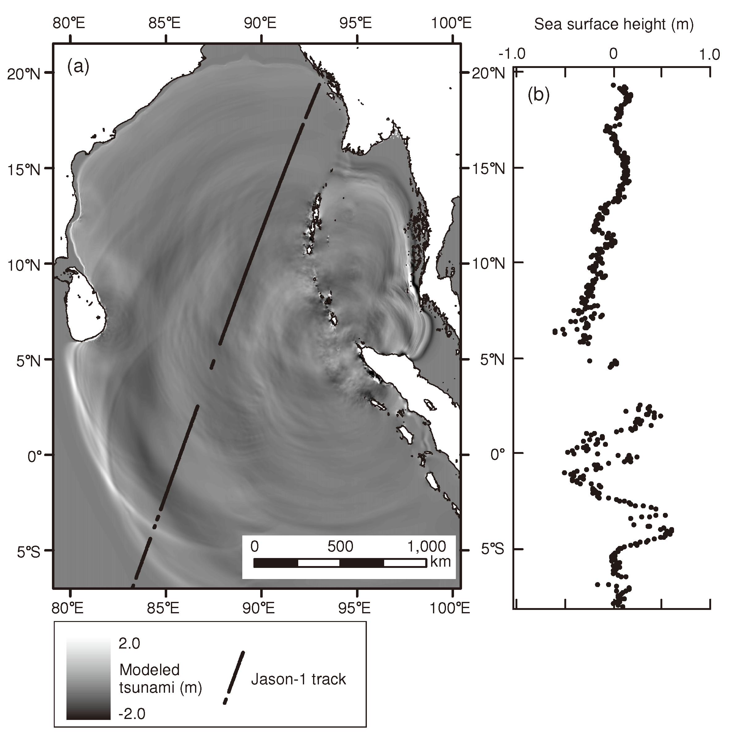
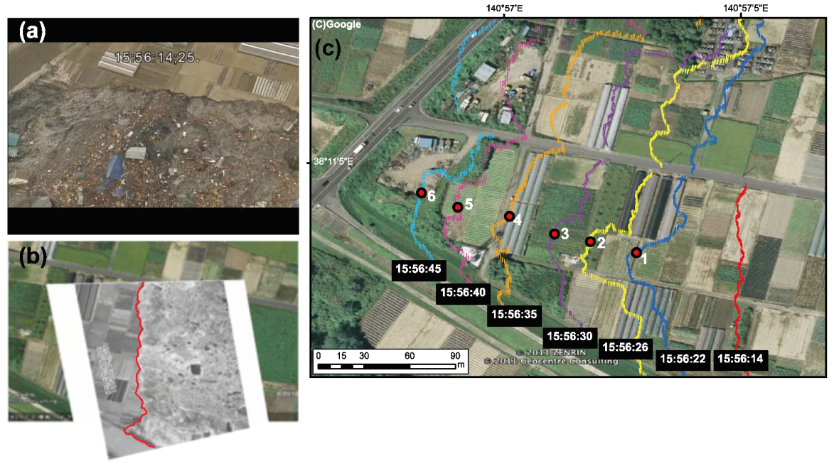
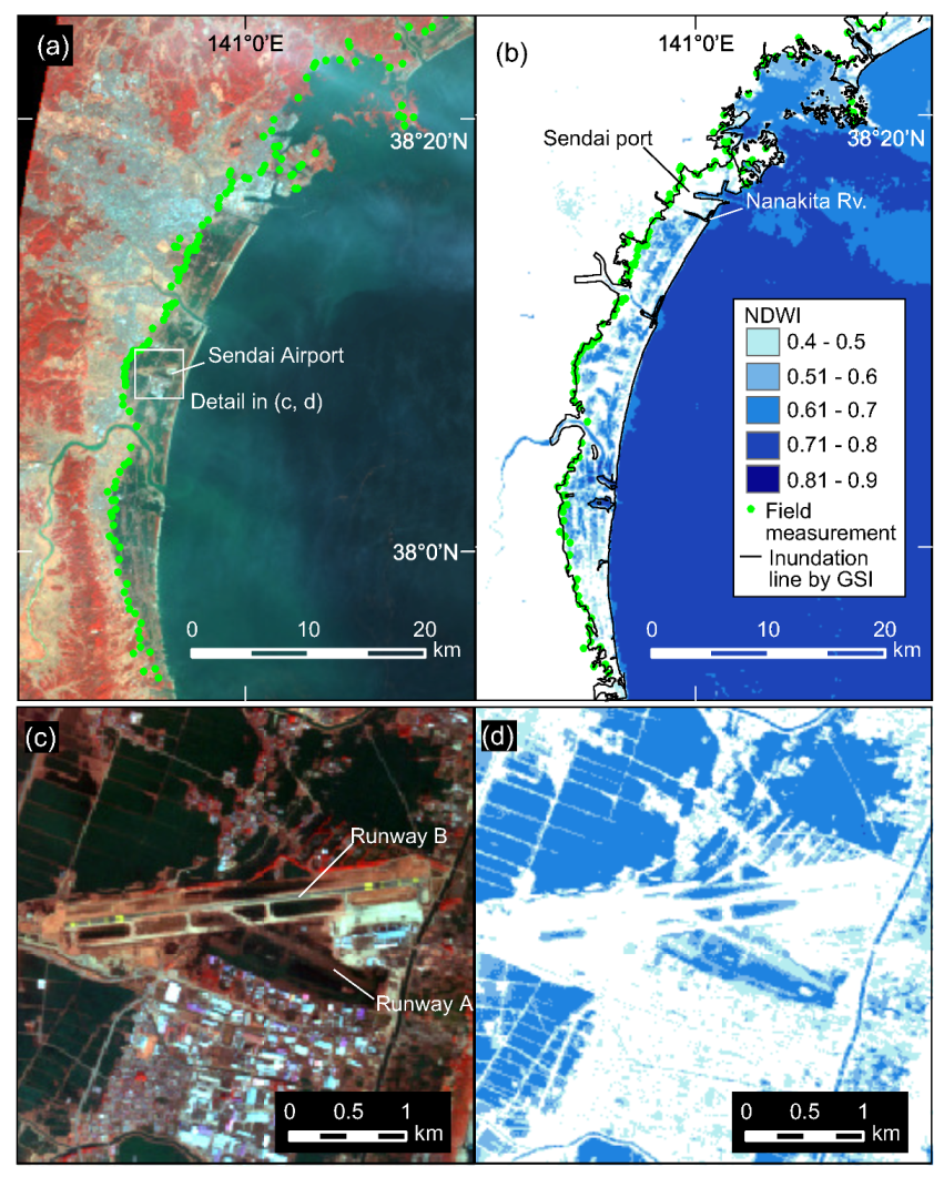
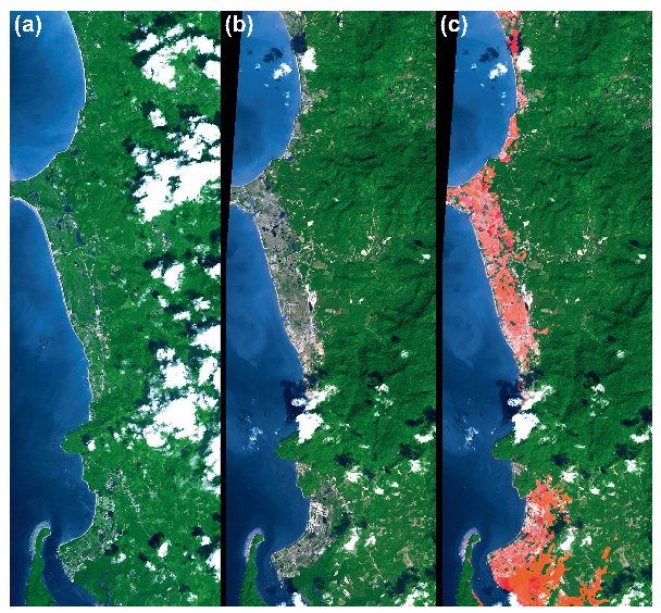
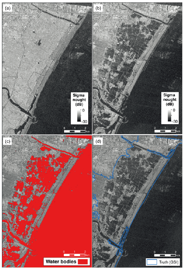
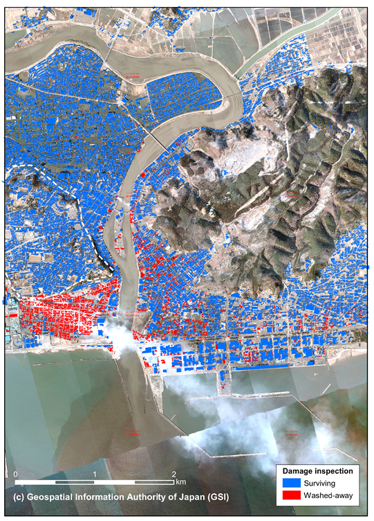
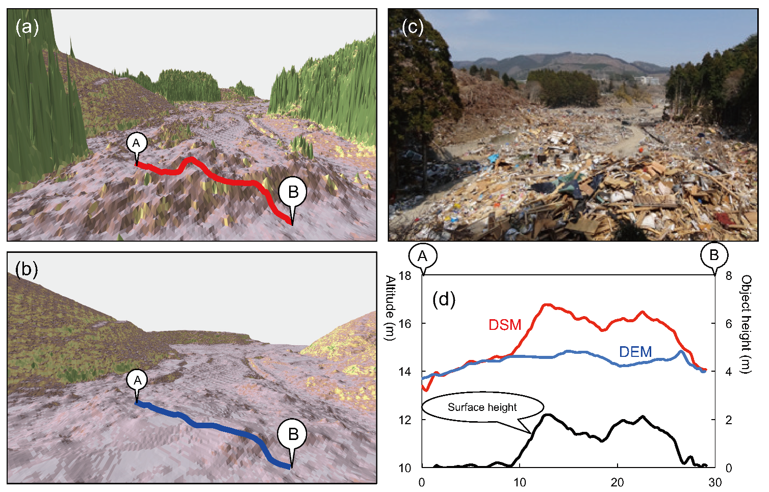
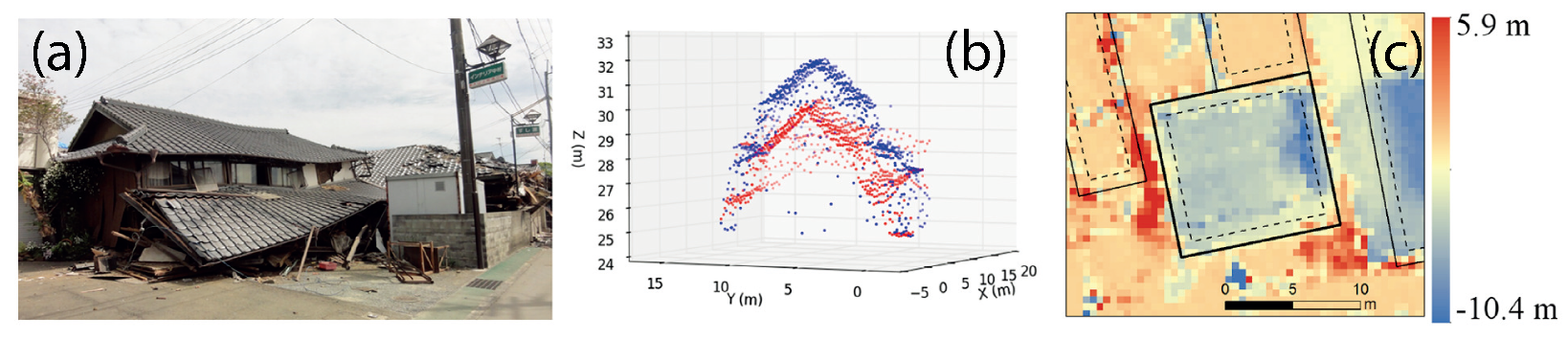
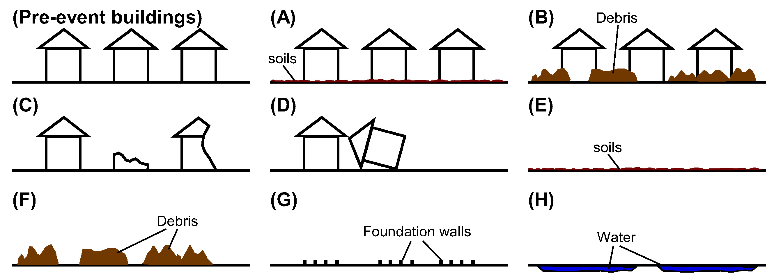
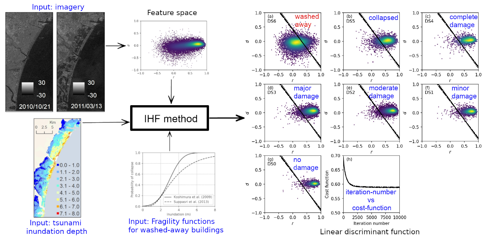
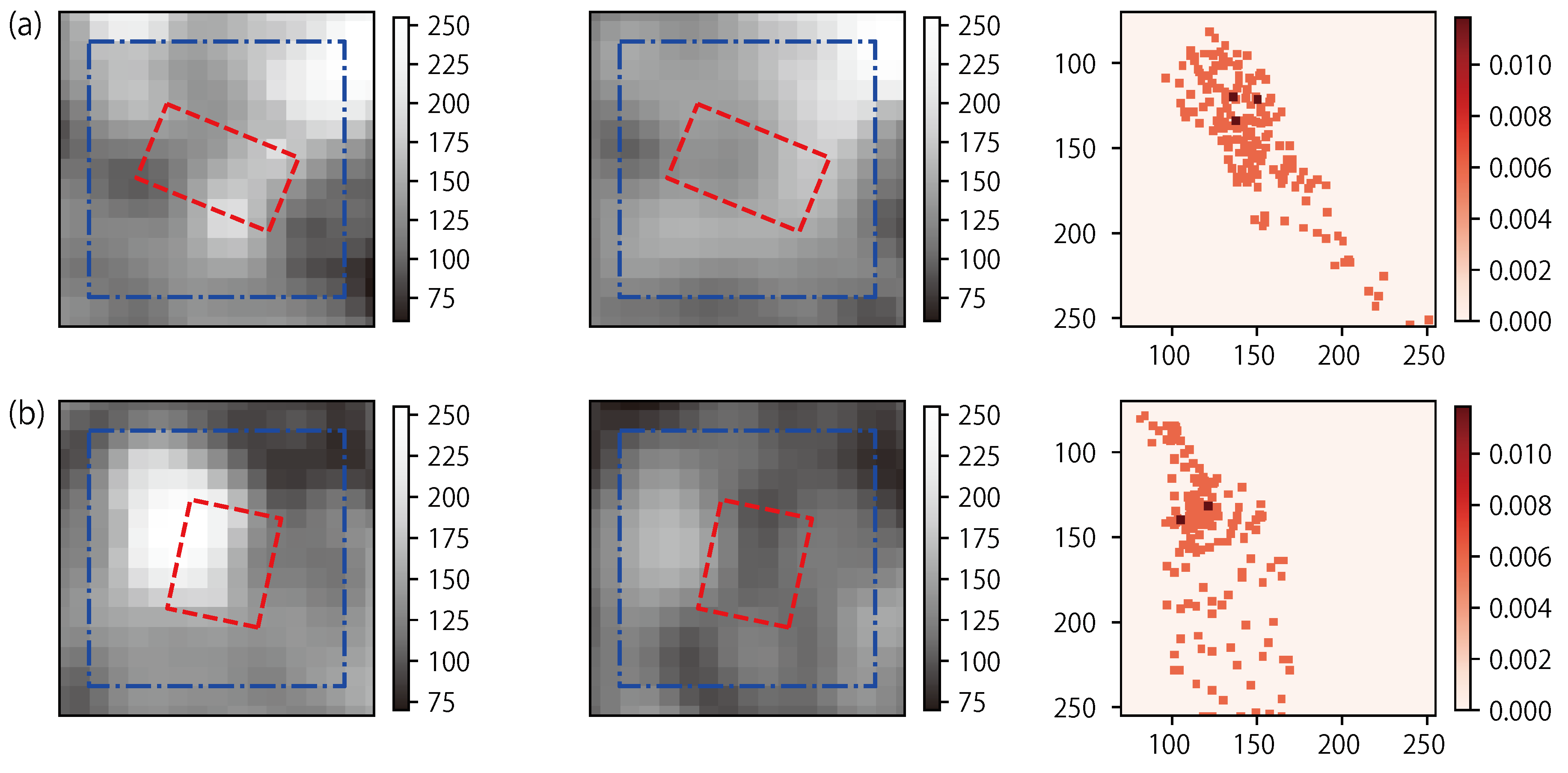
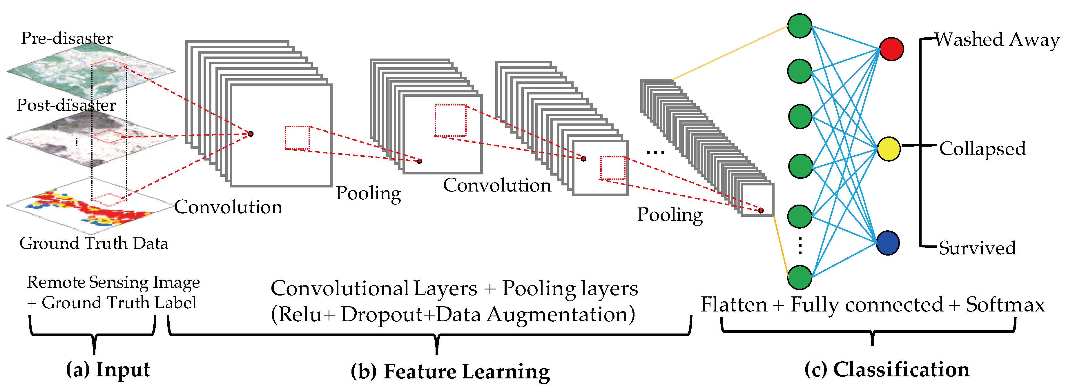
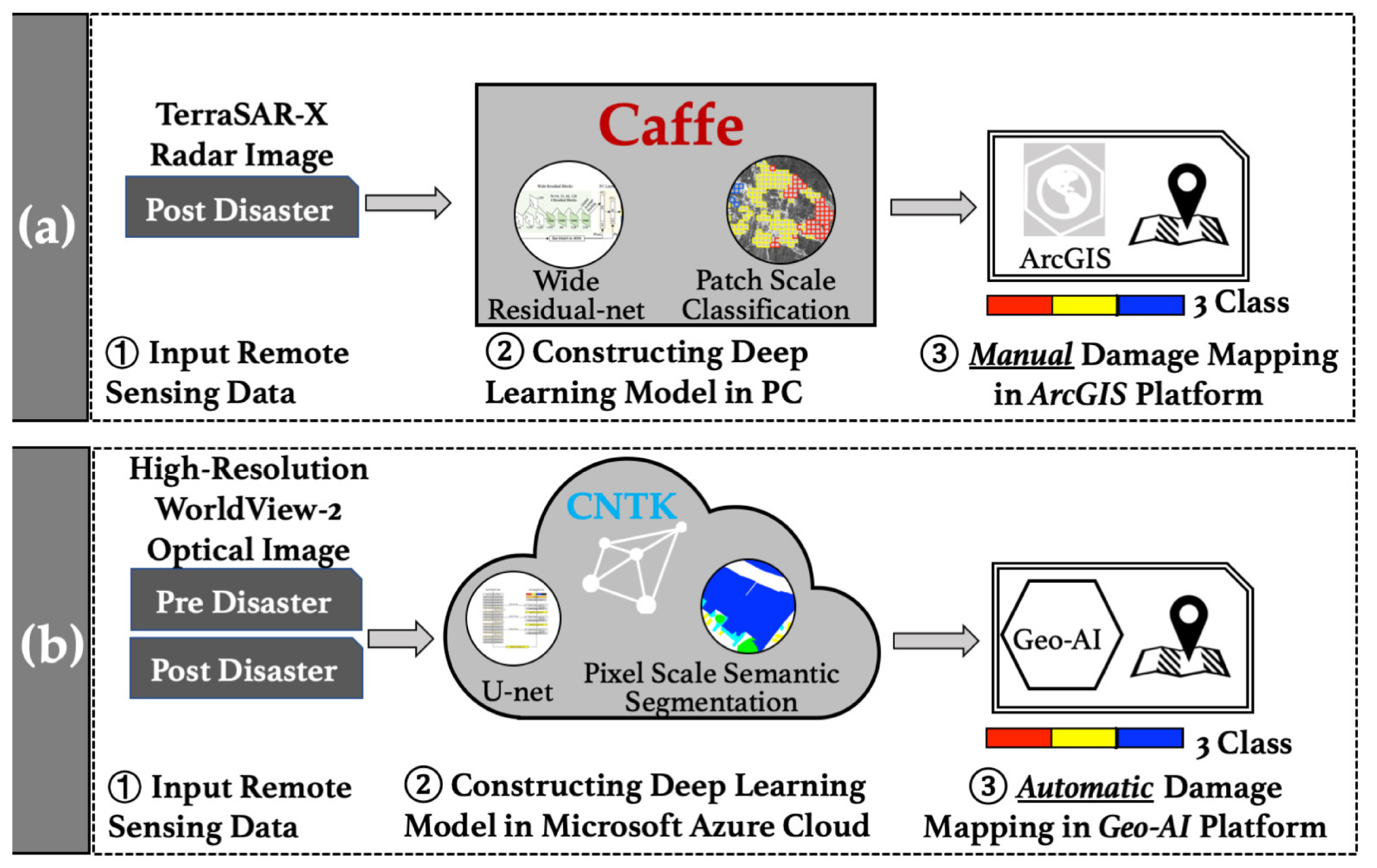
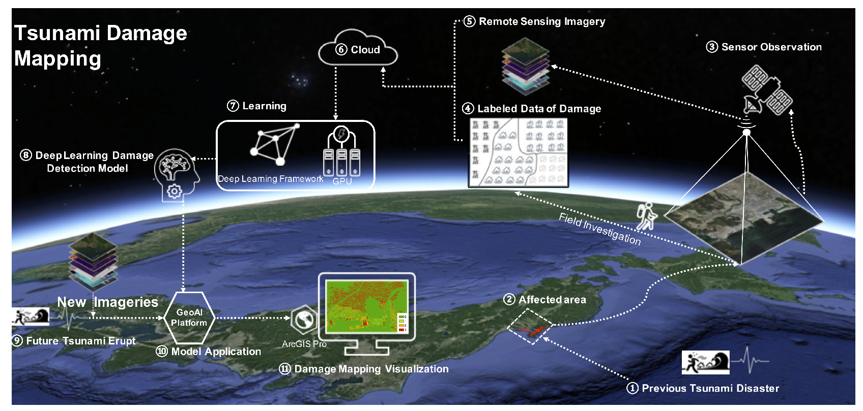
Table 1.
Tsunami features acquired with remote sensing platforms and sensors.
| Tsunami Features | Platforms | Sensors/Sensing Methods |
|---|---|---|
| Mid-ocean propagation | Satellites | Altimeter (Sea surface level) |
| Inland penetration | Aircrafts | Videos |
| Inundation zone | Satellites, Aircrafts | Optical sensors, SAR |
| Structural damage | Satellites, Aircrafts Drones | Optical sensors, SAR |
| Debris | Satellites, Aircrafts, Drones | Optical sensors, SAR, LiDAR |
| Search and rescue | Aircrafts, Drones | Optical sensors, Videos |
Table 2.
A list of tsunami disaster events and the remote sensing-based research related to it.
| Event | Reference |
|---|---|
| 2004 Indian Ocean | [9,24,29,30,31] |
| 2007 Pisco, Peru | [32,33] |
| 2009 American Samoa, US | [34,35] |
| 2010 Maule, Chile | [36] |
| 2011 Tohoku, Japan | [10,16,22,23,34,37,38,39,40,41,42,43,44,45,46,47,48,49,50,51,52,53,54] |
| 2018 Sulawesi, Indonesia | [55,56] |
Table 3.
Summary of the studies related to tsunami damage identification using machine learning algorithms. Abbreviations are as follows: 2004IO = 2004 Indian Ocean tsunami, 2011T = 2011 Tohoku tsunami, OA = overall accuracy, NA = not available.
Table 3.
Summary of the studies related to tsunami damage identification using machine learning algorithms. Abbreviations are as follows: 2004IO = 2004 Indian Ocean tsunami, 2011T = 2011 Tohoku tsunami, OA = overall accuracy, NA = not available.
| Input | Event | Degree of Automation | Metric | Accuracy | Reference |
|---|---|---|---|---|---|
| Radarsat-1 | 2004IO | automatic | OA | 0.95–0.99 | [78] |
| VNIR | 2011T | required visual inspection | NA | NA | [53] |
| ALOS-2 Polarimetric SAR | 2011T | automatic | g-mean | 0.27–0.90 | [86] |
| SAR, demand, fragility function | 2011T | automatic | F1 | 0.80–0.85 | [49] |
| TerraSAR-X, ALOS-2 | 2011T | required training data | F1 | 0.62–0.86 | [91] |
| TerraSAR-X | 2011T | required training data | F1 | 0.62–0.71 | [48] |
| TerraSAR-X | 2011T | required training data | F1 | 0.80–0.91 | [52] |
| TerraSAR-X | 2011T | required training data | OA | 0.67 | [45] |
| Planet, ALOS-2, Sentinel-1, 2 | 2018S | required training data | OA | 0.83–0.92 | [55] |
| Planet, Sentinel-2, urban footprint data | 2018S | required training data | OA | 0.85 ± 0.06 | [56] |
Table 4.
Summary of the studies related to the 2011 Tohoku tsunami damage identification using deep learning algorithms. Abbreviations for damage class are as follows: WA = Washed-away, C = Collapsed, S = Surviving.
Table 4.
Summary of the studies related to the 2011 Tohoku tsunami damage identification using deep learning algorithms. Abbreviations for damage class are as follows: WA = Washed-away, C = Collapsed, S = Surviving.
| Network Structure | Input Data | Accuracy | Damage Class | Reference |
|---|---|---|---|---|
| AlexNet and VGG | Aerial Photo | 0.94–0.96 | WA, S | [54] |
| Wide residual networks [89] | TerraSAR-X (SAR) | 0.75 | WA, C, S | [102] |
| U-net | WorldView-2 (Optical) | 0.71 | WA, C, S | [50] |
© 2020 by the authors. Licensee MDPI, Basel, Switzerland. This article is an open access article distributed under the terms and conditions of the Creative Commons Attribution (CC BY) license (http://creativecommons.org/licenses/by/4.0/).
Share and Cite
MDPI and ACS Style
Koshimura, S.; Moya, L.; Mas, E.; Bai, Y. Tsunami Damage Detection with Remote Sensing: A Review. Geosciences 2020, 10, 177. https://doi.org/10.3390/geosciences10050177
AMA Style
Koshimura S, Moya L, Mas E, Bai Y. Tsunami Damage Detection with Remote Sensing: A Review. Geosciences. 2020; 10(5):177. https://doi.org/10.3390/geosciences10050177
Chicago/Turabian StyleKoshimura, Shunichi, Luis Moya, Erick Mas, and Yanbing Bai. 2020. "Tsunami Damage Detection with Remote Sensing: A Review" Geosciences 10, no. 5: 177. https://doi.org/10.3390/geosciences10050177
Note that from the first issue of 2016, this journal uses article numbers instead of page numbers. See further details here.