


Multistability and Phase Synchronization of Rulkov Neurons Coupled with a Locally Active Discrete Memristor


1
School of Automation and Electronic Information, Xiangtan University, Xiangtan 411105, China
2
School of Engineering and Technology, University of Hertfordshire, Hatfield AL10 9AB, UK
3
College of Information Science and Engineering, Hunan University, Changsha 410082, China
*
Author to whom correspondence should be addressed.
Fractal Fract. 2023, 7(1), 82; https://doi.org/10.3390/fractalfract7010082
Submission received: 21 November 2022
/
Revised: 5 January 2023
/
Accepted: 7 January 2023
/
Published: 11 January 2023
(This article belongs to the Special Issue Recent Advances in Fractional-Order Neural Networks: Theory and Application)
Abstract
:In order to enrich the dynamic behaviors of discrete neuron models and more effectively mimic biological neural networks, this paper proposes a bistable locally active discrete memristor (LADM) model to mimic synapses. We explored the dynamic behaviors of neural networks by introducing the LADM into two identical Rulkov neurons. Based on numerical simulation, the neural network manifested multistability and new firing behaviors under different system parameters and initial values. In addition, the phase synchronization between the neurons was explored. Additionally, it is worth mentioning that the Rulkov neurons showed synchronization transition behavior; that is, anti-phase synchronization changed to in-phase synchronization with the change in the coupling strength. In particular, the anti-phase synchronization of different firing patterns in the neural network was investigated. This can characterize the different firing behaviors of coupled homogeneous neurons in the different functional areas of the brain, which is helpful to understand the formation of functional areas. This paper has a potential research value and lays the foundation for biological neuron experiments and neuron-based engineering applications.
1. Introduction
The brain is regarded as a complex neural network composed of many neurons. Information transmission [1,2,3] and conscious perception [4] are closely related to the dynamical behaviors of biological neural networks. At the same time, synchronization plays a role in some pathologies in neuroscience, such as epilepsy. Experiments [5,6] showed that the nervous system exhibited high synchronization during seizures. In order to better understand the structure of the brain, researchers have studied a large number of dynamic characteristics of neural networks [7,8,9,10,11,12]. However, continuous neuron models have the characteristics of high dimension and multiscale, which are not conducive to the study of complex and large-scale neural networks. In recent years, discrete neuron models have drawn more attention due to their simple form and flexible calculation. Extensive studies [13,14,15,16,17,18] proved that discrete neuron models, especially the Rulkov neuron, could more effectively mimic the real behaviors of biological neurons. On this foundation, Cao et al. [19,20,21,22,23] disclosed two identical Rulkov neurons coupled with chemical and electrical synapses, respectively, and reported the influence of the coupling strength on synchronization in detail. By constructing a small-world network made up of Rulkov neurons, Ferrari et al. [24] proposed the idea of using delayed feedback to suppress synchronization. Rakshit S et al. [25] revealed several types of firing patterns and synchronous behavior of Rulkov neurons under the joint effect of internal connections and a chemical synapse.
In 1971, Chua first put forward the concept of a memristor as a device to describe the relationship between the charge and the flux [26]. Since HP Laboratory developed the entity of memristor in 2008 [27], continuous memristors have been widely used in neural networks [28,29,30,31,32,33,34] and neural morphological circuits [35,36,37,38,39]. Ding et al. [40] studied the hidden coexisting firing patterns of two heterogeneous fractional-order HR neurons coupled with a memristor and applied them to image encryption. However, the synchronization between the neurons was not analyzed. Because of the properties of memorability, nonvolatility, nanoscale, and local activity, memristors are regarded as the best choice to mimic synapses, which have been proved in continuous neuron models. Additionally, phenomena such as coexisting firing patterns [41,42,43,44] and synchronization [45,46,47] have been found. It was found in [48] that anti-phase synchronization helps to distinguish the different functional areas of the brain. However, the anti-phase synchronization of different firing patterns was not found. Recently, researchers have shifted their focus to discrete memristors. Introducing discrete memristors to different maps, it was found that discrete memristive chaotic systems have the advantages of high complexity [49,50,51], coexisting attractors [52,53,54], and offset boosting [55]. Furthermore, Peng et al. [56] also studied parameter identification for discrete memristive chaotic maps. In addition, it was found in [57] that the integer-order discrete memristor has an ideal memory effect, whereas the fractional-order discrete memristor does not.
As far as we know, there is very little discussion about discrete memristors in the field of neural networks, and currently, it basically stays at the single-neuron coupling stage. For example, it was revealed in [58,59,60] that the introduction of discrete memristors could enrich the firing patterns of neurons, and phenomena such as hyperchaotic firing and regime transition were surveyed. Lu et al. [61] studied the dynamic characteristics of Rulkov neurons under electromagnetic induction by introducing a discrete memristor and found that the dynamic behaviors of fractional-order systems are more complex than that of integer-order systems. However, compared with integer-order systems, the calculation cost of fractional-order systems is higher. Xu et al. [62] discovered coexisting firing behaviors by introducing a memristor to a single continuous nonautonomous Rulkov neuron. However, the firing pattern of this system was of a relatively single type. Li et al. [63] reported hidden attractors and coexisting firing patterns in a discrete memristive synapse-coupled single HR neuron model. It can be seen that it is very meaningful to introduce discrete memristors into discrete neuron models.
Inspired by the above literature, we investigate the firing behaviors and phase synchronization of two Rulkov neurons coupled with the LADM in this paper. The main contributions are summarized as follows:
- (1)
- Compared with the original neurons, the Rulkov neurons coupled with the LADM produce many novel firing patterns. Meanwhile, we show the coexisting firing behaviors of the neural network;
- (2)
- The synchronization transition behavior is explored;
- (3)
- The neural network exhibits the anti-phase synchronization of different firing patterns of homogeneous neurons, which has not been found in the previous literature.
The remaining structure of this paper is as follows: Section 2 shows the new bistable LADM model, and its characteristics of nonvolatility, bistability, and local activity are verified through numerical simulation. In Section 3, the Rulkov neuron model coupled with LADM is established. Then, we discuss the influence of the LADM on the firing behavior of discrete neurons in Section 4. The synchronization behaviors between the neurons are reported in Section 5, and finally, the conclusions are given in Section 6.
2. Bistable LADM Model
2.1. Pinched Hysteresis Loops and Bistability
In this paper, we propose a new LADM, specifically described as
In Equation (1), i(n) and v(n) represent the output current and input voltage of the LADM, W(ϕ) is the memductance, and β, γ, δ are memristive parameters. In this paper, we let β = 0.1, γ = −0.1, and δ = 11.
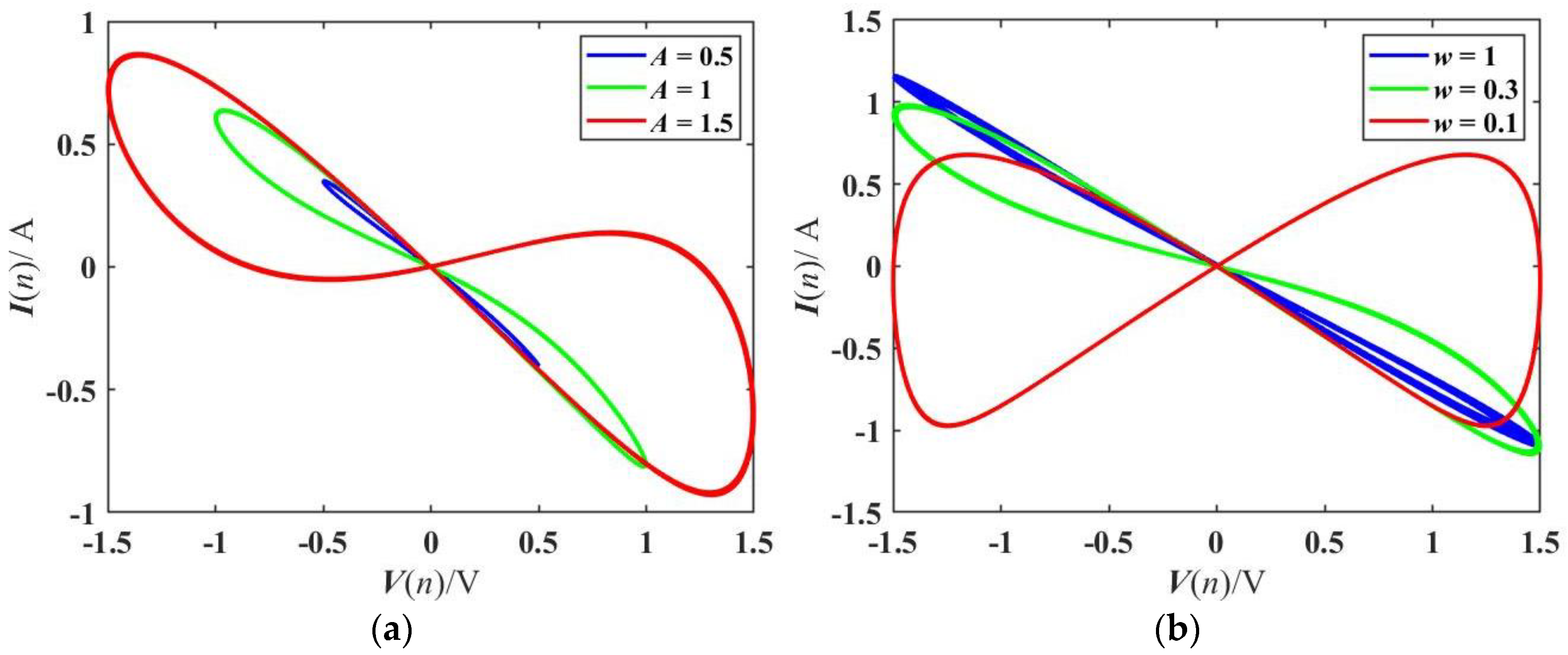
A sinusoidal voltage signal v(n) = Asin(wT(n)) is added, and the volt-ampere characteristic curves of the LADM are shown in Figure 1. Changing the amplitude, it can be seen from Figure 1a that the pinched hysteresis loops through the origin present an oblique “8” shape, and the area of the loops gradually becomes larger as the amplitude increases. The corresponding pinched hysteresis loops can be observed in Figure 1b as the frequency varies from 0 to 1. When the frequency is small, the pinched hysteresis loop is located in all quadrants. When the frequency increases, the pinched hysteresis loop area decreases and is gradually limited to the second and fourth quadrants. Finally, it is a negative single-valued function, namely a negative resistance. Thus, the LADM meets the definition of a memristor [64].
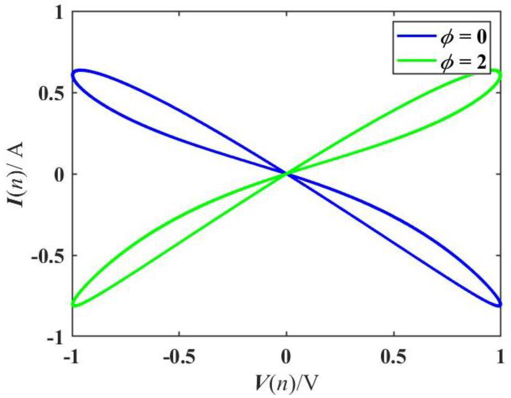
A multistable memristor refers to a memristor with multiple coexisting stable pinched hysteresis loops under different initial values [65]. As shown in Figure 2, with frequency w = 0.2 Hz and amplitude A = 1 V, when the two internal initial states are set as ϕ(0) = 0 and ϕ(0) = 2, respectively, there are two different pinched hysteresis loops on the V–I phase plane, which means that the LADM is bistable.
2.2. Nonvolatility and Local Activity
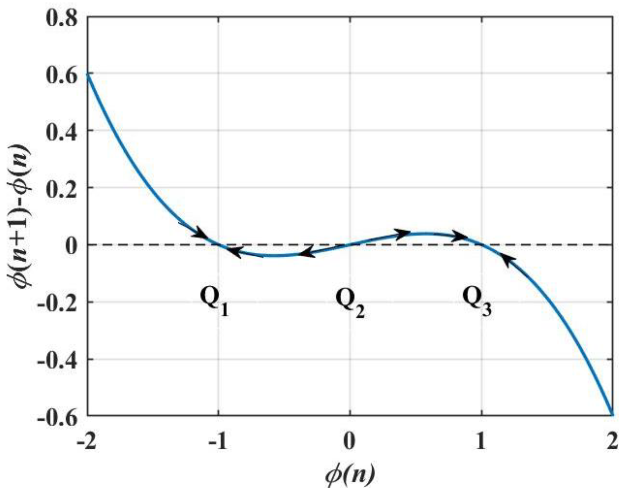
The nonvolatile property of the memristor allows the memristor to remain up-to-date when the power is off, which can be characterized by the power-off plot (POP) [66], i.e., the existence of two or more negative slopes intersecting the ϕ-axis. Letting v(n) = 0, the equilibrium equation can be obtained as follows:
The dynamic curve of Equation (2) is drawn in Figure 3. According to the direction of the arrows shown in Figure 3, we can judge what state the internal state variable will eventually stabilize in different situations. It shows that the intersection points of the curve and ϕ-axis are Q1 (−1, 0), Q2 (0, 0), and Q3 (1, 0), respectively. Q1 and Q3 are the two intersection points with negative slopes. Therefore, the nonvolatile memristor has two stable states under different initial states, that is to say,
According to the above analysis, it can be concluded that the memristor is nonvolatile.
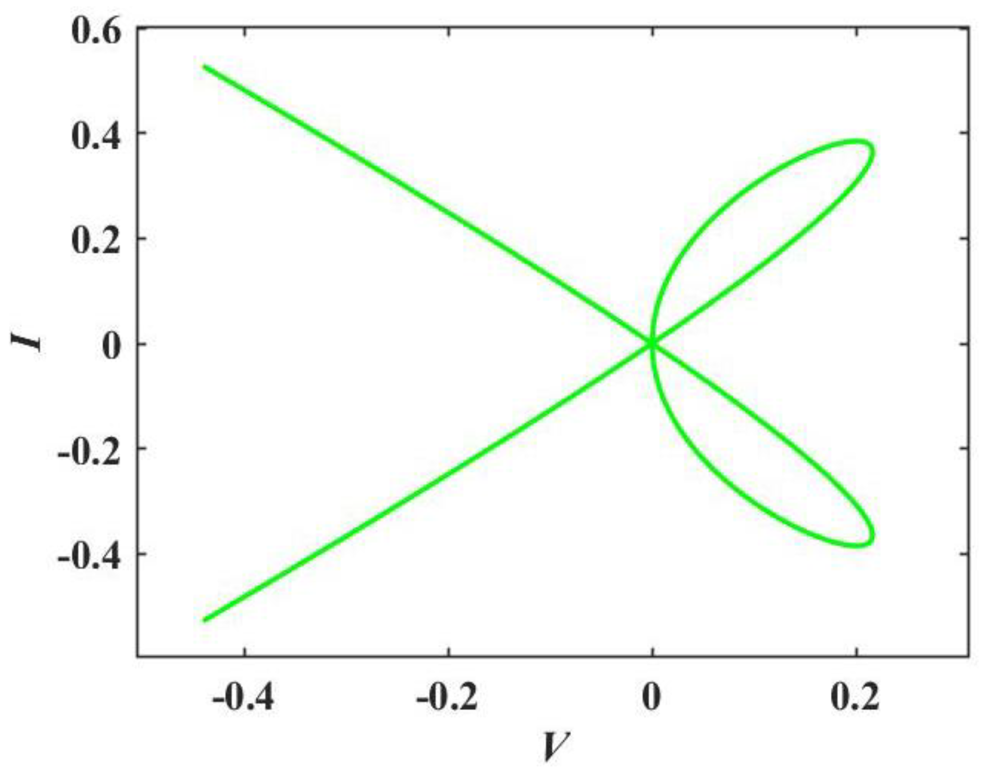
Local activity is the root of complexity [67]. The locally active nature of the memristor can be judged by the DC V–I diagram, i.e., the existence of at least one negative slope curve of the diagram [64]. For a better illustration, let ϕ(n + 1) − ϕ(n) = 0, which gives the equilibrium equation
In Equation (4), V is the DC voltage, I is the DC current, and Φ implies a variable equilibrium state of the equation and satisfies ϕ(n + 1) − ϕ(n) = 0, ϕ(n) = Φ. Taking the range of Φ as [−2, 2], the curve of the V–I plane is drawn in Figure 4, and it is clear that the memristor has two locally active regions. Then, the LADM has the characteristic of local activity.
3. The Neural Network Model and Equilibrium Point Analysis
The Rulkov neuron has the following main firing patterns: period-1 bursting firing, triangular bursting firing, square-wave bursting firing, etc. By coupling two Rulkov neurons with the proposed LADM, we can obtain a new LADM-based integer-order Rulkov neural network (IORNN) model as
where x1 and x2 denote the membrane potentials of neurons; y1 and y2 are the neuronal recovery variables; (x1(n) − x2(n)) means the membrane potential difference between two Rulkov neurons; αi (i = 1, 2), αi, and σ are parameters controlling the firing patterns of neurons, 0 < μ ≪ 1; and k represents the coupling strength. What needs to be noted is that the control parameters of the new neural network are fixed with μ = 0.001 and σ = −1 in this paper [68].
It is known that the equilibrium points for calculating Equation (5) are E1 (σ, σ − α1/(1 + σ2), σ, α2/(1 + σ2), 1), E2 (σ, σ − α1/(1 + σ2), σ, α2/(1 + σ2), −1), and E3 (σ, σ − α1/(1 + σ2), σ, α2/(1 + σ2), 0). For E3, the Jacobi matrix is calculated as
The eigenvalues can be obtained from , where is an identity matrix. For the convenience of calculation, we assume that α1 = α2.
It is obvious that there is a constant λ = 1.1 > 1, so E3 is always unstable. In the following numerical simulation, it can be inferred that unstable points will lead to chaos. Similarly, for E1 and E2, it can be calculated that the eigenvalues are the same, both of which are (0.8, 1, −0.5α, 1, −0.5α). Additionally, it is valid when the control parameter α is positive for the neural network. Therefore, the equilibrium points E1 and E2 are stable.
Discrete fractional calculus is suggested to describe neural networks with memory effects [69,70]. In order to present the fractional-order model, some definitions and lemmas are given below.
Definition 1.
Following [61], for a given fractional-order q > 0, , when x(t) is defined in , its Caputo difference is defined by
where Γ(·) is the gamma function,,= {t0, t0 + 1, t0 + 2, · · ·}, m = [q], and ρ(s) denotes the next point in the time scale after s, namely ρ(s) = s + 1 for. Obviously, when q = 1, the fractional difference becomes.
Theorem 1.
Following [61], for the Caputo-like fractional-order system,
The definition can continue to be equivalent to the equation
Furthermore, let s + q = j; then, the equation can be changed to
where x(t) is the system variable, and g(·) is the system equation.
Based on the Caputo fractional-order difference operator and Equation (5), we can obtain a new LADM-based fractional-order Rulkov neural network (FORNN) model as
where x1(0) and x2(0) denote the initial membrane potentials of neurons, y1(0) and y2(0) are the initial neuronal recovery variables, and q is the fractional order. Other parameters are the same as those in Equation (5).
4. Multistability and Novel Firing Patterns
Some simulation results are presented in this section. These results indicate that the introduction of the LADM improves the complexity of neurons, and the firing states of the neural network can be selected by adjusting the initial values or the coupling strength k, which has a potential application value in engineering applications.
4.1. Transition of Firing Patterns
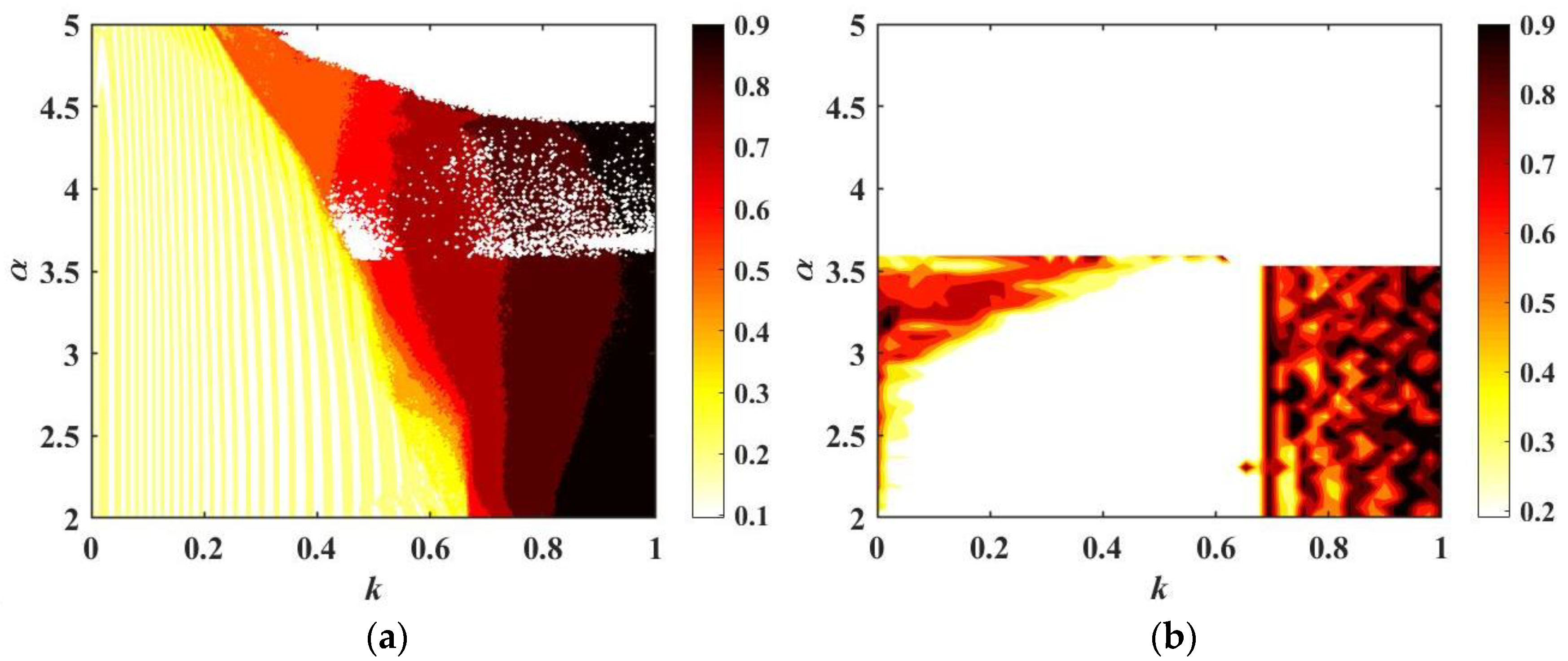
According to [25], it is assumed that the two neurons have the same firing patterns before coupling, which means α = α1 = α2. As the control variable α of a neuron is set in the range of [2, 5], and the coupling strength k is varied from 0 to 1, the spectral entropy complexity [71] of the IORNN and FORNN are shown in Figure 5. Different colors represent different degrees of complexity, and the darker the color, the more complex it will be. Brown and black imply chaotic or hyperchaotic firing patterns, and yellow indicates periodic firing behaviors. The diversity of colors indicates that neurons have rich firing behaviors, and the transition of firing patterns can be expressed by the variation in the colors with the change in the coupling strength. It is obvious that the types of firing patterns of the FORNN at q = 0.6 are less than those of the IORNN. Here, a few examples are presented to illustrate this point.
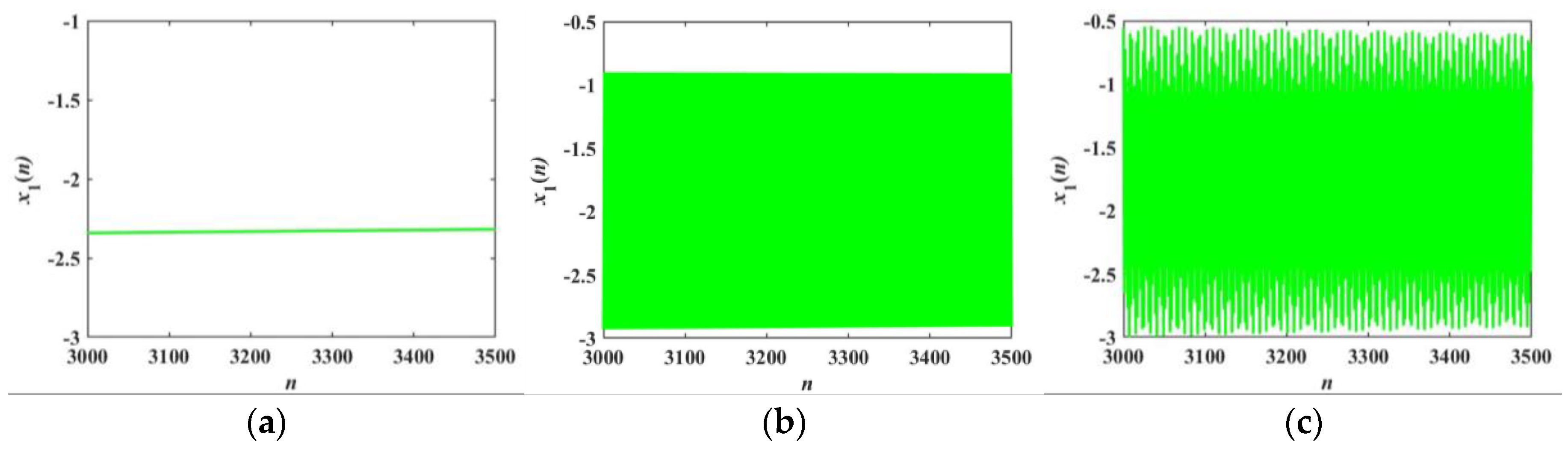
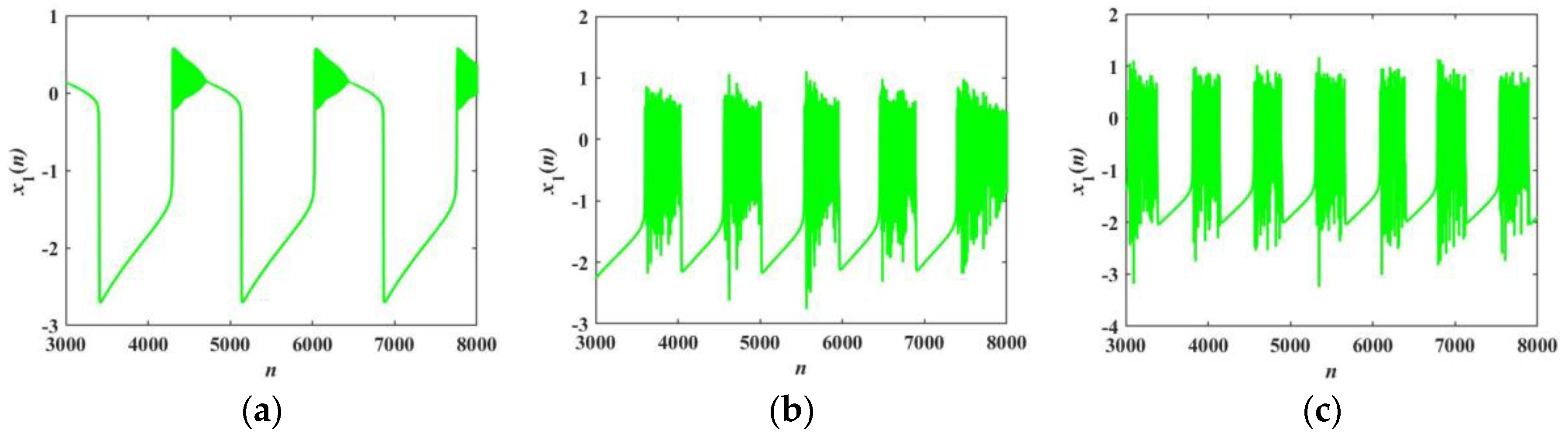
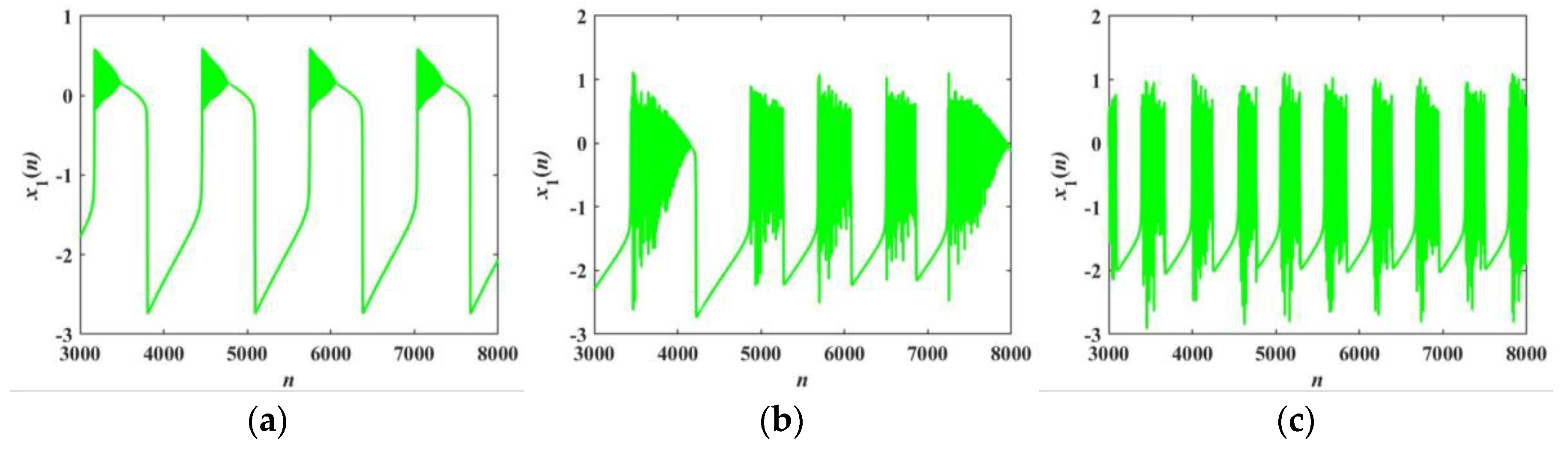
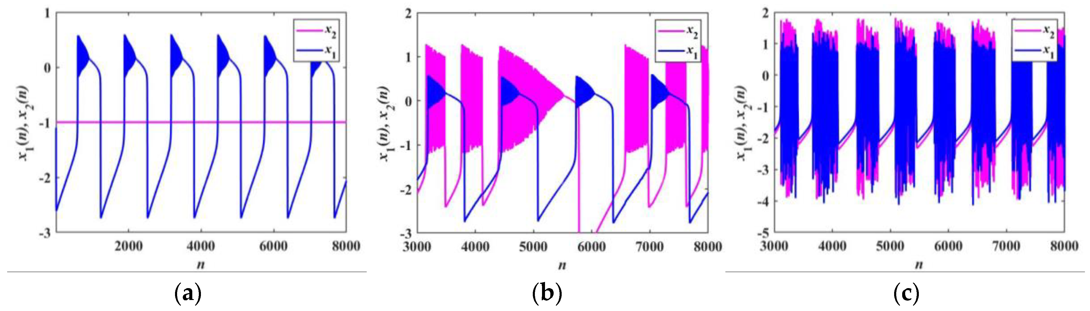
For α = α1 = α2 = 3, the time sequences of the membrane potential x1 under different coupling strengths are depicted in Figure 6, Figure 7 and Figure 8. The firing patterns of the FORNN are shown in Figure 6 and Figure 7, while the firing patterns of the IORNN are presented in Figure 8. When the fractional order q = 0.6, and the coupling strength k varies from 0 to 1, a transition occurs from a silent state to silent firing and periodic spike firing. When the fractional order is 0.95, it can be seen that the firing patterns of the FORNN are basically the same as that of the IORNN. The periodic triangular bursting firing pattern is drawn in Figure 8a. However, in Figure 8b, the neurons exhibit a mixed firing pattern with chaotic triangular bursting firing and square-wave bursting firing. When k = 0.8, the neurons exhibit chaotic square-wave bursting firing, as presented in Figure 8c. In addition, the transition process corresponds to the SE complexity in Figure 5.
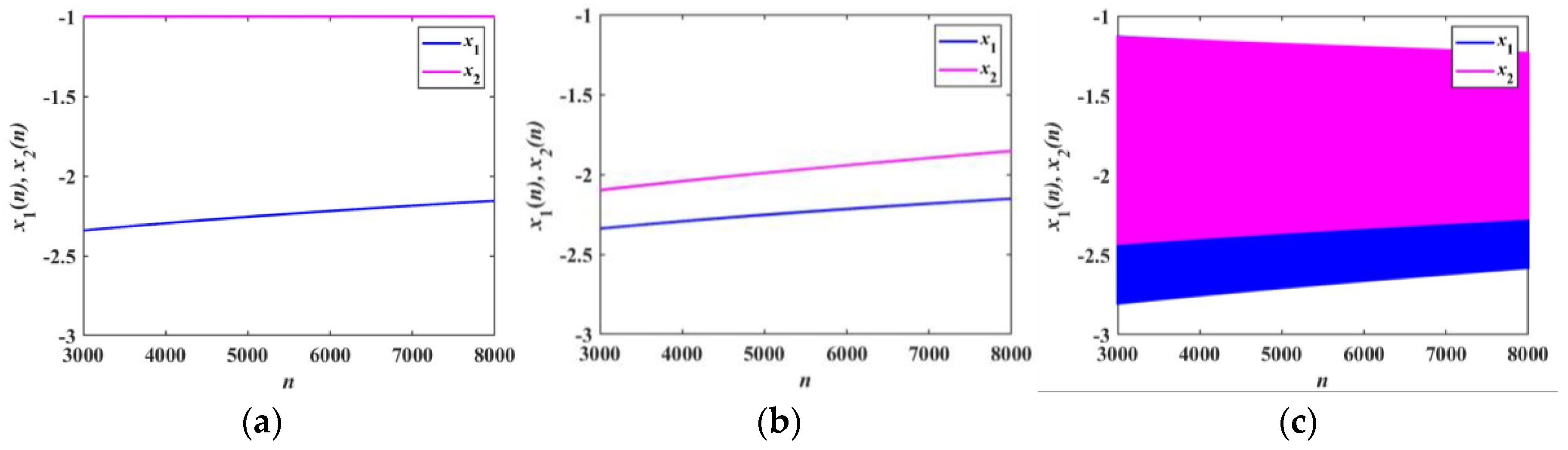
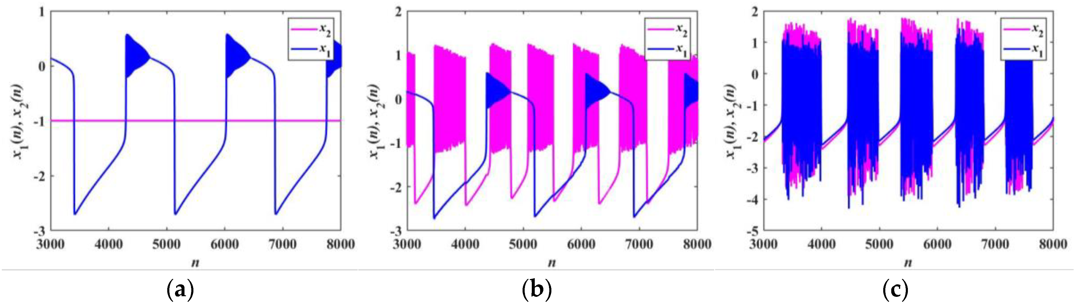
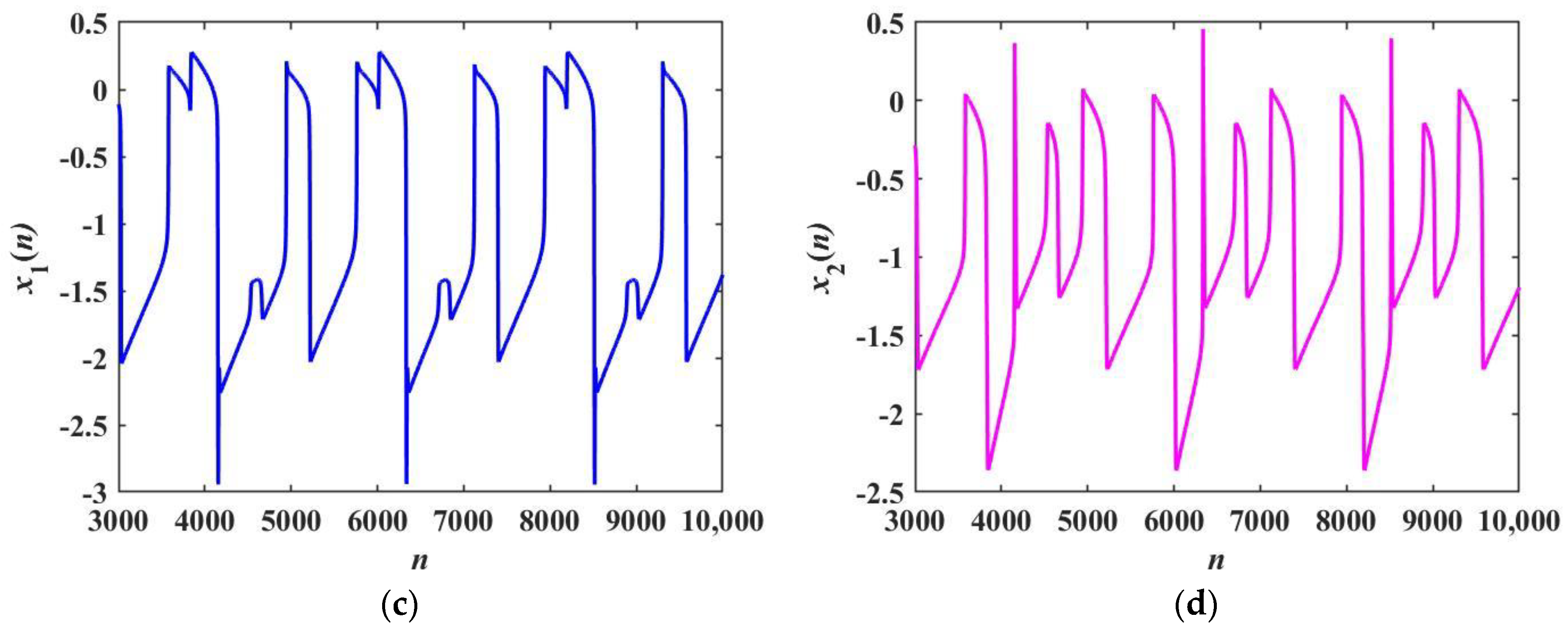
In Figure 9, Figure 10 and Figure 11, the blue dots and lines indicate the membrane potential x1, while the magenta dots and lines indicate the membrane potential x2. Figure 9 and Figure 10 show the transition process of the firing patterns of the FORNN with α1 = 3 and α2 = 4. With q = 0.6, k = 0, and k = 0.01, as plotted in Figure 9a,b, the membrane potentials x1 and x2 are in a silent state. When k = 0.8, the firing patterns of the neurons are periodic firing, as presented in Figure 9c. Similarly, when q = 0.95, the firing patterns of the FORNN are basically the same as that of the IORNN shown in Figure 10 and Figure 11. Figure 11 shows the transition process of the firing patterns of the IORNN with α1 = 3 and α2 = 4. As shown in Figure 11a, the membrane potential x2 is in a silent state, while the membrane potential x1 is in a triangular bursting firing state at k = 0. With a slight increase in the coupling strength, the membrane potential x2 shown in Figure 11b starts to excite as a mixed firing pattern, which indicates that a synapse acts as an intermediary to successfully transmit information between neurons. In Figure 11c, the two Rulkov neurons reach synchronization at k = 0.8. It is clear that the coupling strength plays a decisive role in regulating the firing states of neurons, which also indicates that synaptic modulation plays an important role in the synchronization process.
It is found that the firing patterns of the LADM-based FORNN are more complex than that of the LADM-based IORNN, but the dynamic behaviors of the IORNN are more convenient to characterize the information transmission process between biological neurons with lower computation costs. Therefore, we will specify the dynamics of the IORNN model in the next section.
4.2. Novel Firing Patterns
Due to the nonvolatile and bistable advantages of the proposed LADM, the bidirectional memristive synapse-coupled neural network leads to novel firing patterns as well as mixed firing patterns, enriching the dynamical behaviors of neurons.
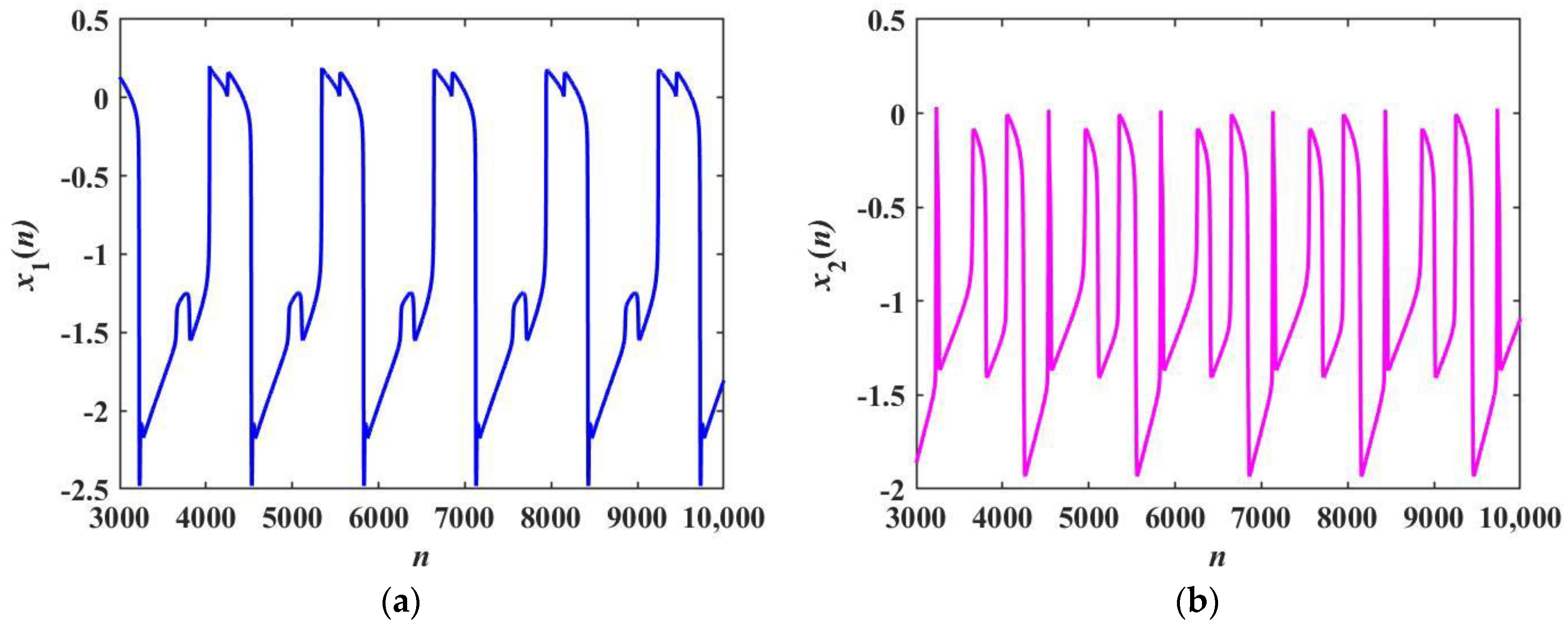
Figure 12 depicts the time sequences of the two membrane potentials x1 and x2 with different coupling strengths, respectively, and blue represents the membrane potential x1, while magenta represents the membrane potential x2. When α1 = 2.5, α2 = 2, and k = 0.1, a new periodic bursting firing pattern appears in Figure 12a, and its topological structure is different from the original Rulkov neuron. With the increase in the coupling strength to 0.2, a crossed firing pattern with different topologies of the bursting firing behavior is shown in Figure 12c. In Figure 12b,d, the membrane potential x2 shows a mixed firing behavior of spike firing and bursting firing. With the increase in the coupling strength, the frequency of the spike firing pattern decreases. It is obvious that the introduction of the LADM enriches the firing patterns of neurons.
With different control variables, the time series of the neuronal membrane potentials x1 and x2 are depicted in Figure 13. Along with the change in the coupling strength, the membrane potential x1 not only produces novel triangular firing behavior but also generates a mixed firing behavior of triangular bursting firing with different topologies, as shown in Figure 13a–c. More interestingly, Figure 13d–f indicate that the membrane potential x2 has a mixed firing pattern with spike firing, period-1 bursting firing, and triangular bursting firing. The frequency of the triangular bursting firing increases with the increase in the coupling strength. These results lead to a similar conclusion that the introduction of the LADM makes the firing behaviors of Rulkov neurons more complicated.
4.3. Transient Chaotic Firing Behavior
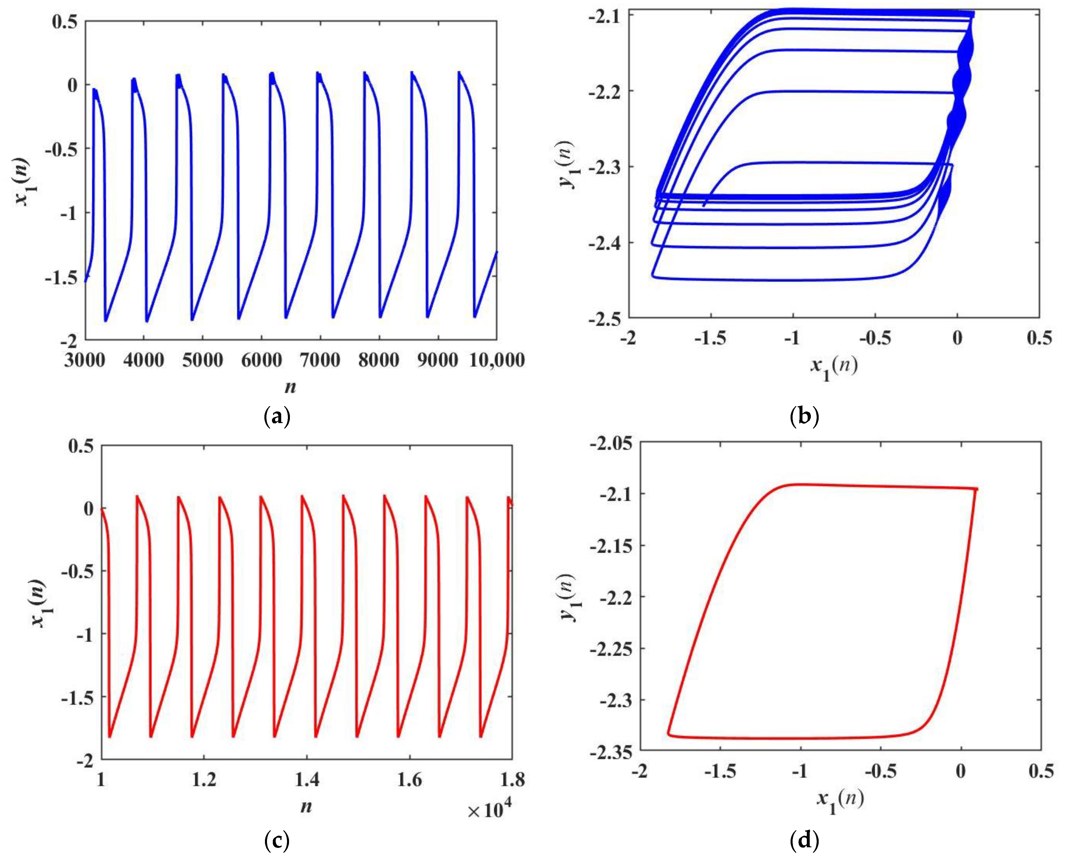
The phase diagrams and time sequences are shown in Figure 14. When α1 = α2 = 2.2, k = 0.5, and the initial values are (−1, 0.5, −1, 0, 0), the membrane potential x1 presents a transient chaotic firing pattern in the time interval n = [3000, 18,000]. The membrane potential x1 shows a chaotic triangular bursting firing pattern in the time interval n = [3000, 10,000]. It is worth noting that the neuron stabilizes into a period-1 bursting firing behavior at n = [10,000, 18,000]. Of course, the iteration times of chaos are different under different initial values.
4.4. Coexisting Firing Patterns
Coexisting behavior is a hot topic in the field of neural networks. The parameters of the neural network are relatively fixed, and the coexisting firing pattern can be obtained only by changing the initial values. The corresponding parameters are assigned as follows: β = 0.1, γ = −0.1, δ = 11, μ = 0.001, σ = −1. Take α1 = α2 = α = 2.2 and α1 = α2 = α= 2.5 as examples, respectively, to reveal two different coexisting firing patterns.
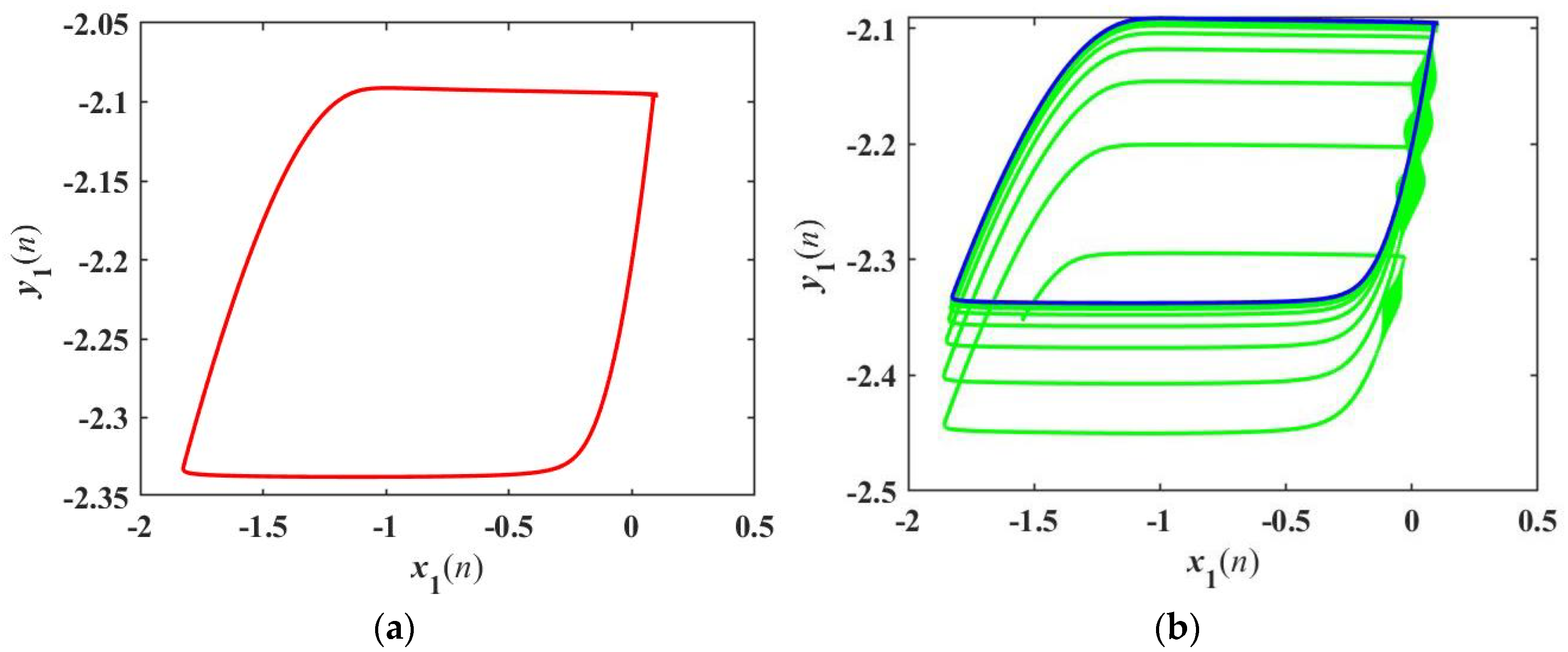
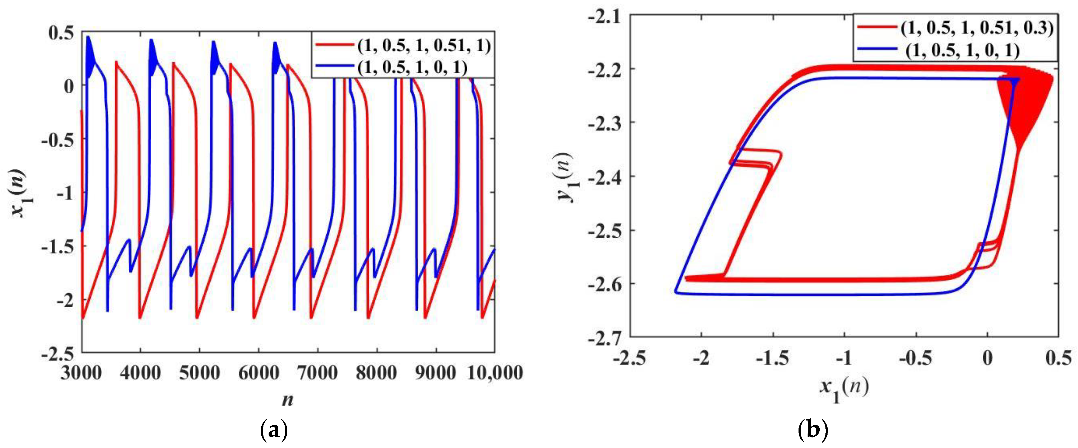
When α = 2.2, and the coupling strength k is set to 0.5, the neuron exhibits the coexisting pattern of periodic and transient chaotic firing. The phase diagrams of the membrane potential x1 under two sets of initial values (x1(0), y1(0), x2(0), y2(0), ϕ(0)) = (−1.1, −3, −1, −3, 0.8) and (−1, 0.5, −1, 0, 0) are drawn in Figure 15. The membrane potential x1, presenting a periodic firing pattern, is shown in Figure 15a. In Figure 15b, the membrane potential x1 presents a transient chaotic firing pattern, and the blue track represents periodic firing, while the green track represents chaotic firing. When α = 2.5, and the coupling strength k is set to 0.1, there is the coexisting behavior of period-1 bursting firing and triangular bursting firing in Rulkov neurons. Figure 16 shows the time series and phase diagrams with different initial values, in which red and blue correspond to the initial values of (1, 0.5, 1, 0.51, 0.3) and (1, 0.5, 1, 0, 1), respectively. It can be seen that when the initial values are chosen as (1, 0.5, 1, 0, 1), the neuron exhibits period-1 bursting firing. When the initial values are changed to (1, 0.5, 1, 0.51, 0.3), the firing pattern switches to triangular bursting firing. It is clear that the multiple firing behaviors of the neural network are very sensitive to the initial values.
5. Phase Synchronization and Synchronization Transition
Each time the neuron begins to burst, the neuronal recovery variable y reaches its maximum value. For a better analysis of phase synchronization, the phase of the recovery variable y is discussed here, giving the definition of phase θ [24]
where nk is the time of the appearance of the kth bursting.
The phase difference can be expressed as
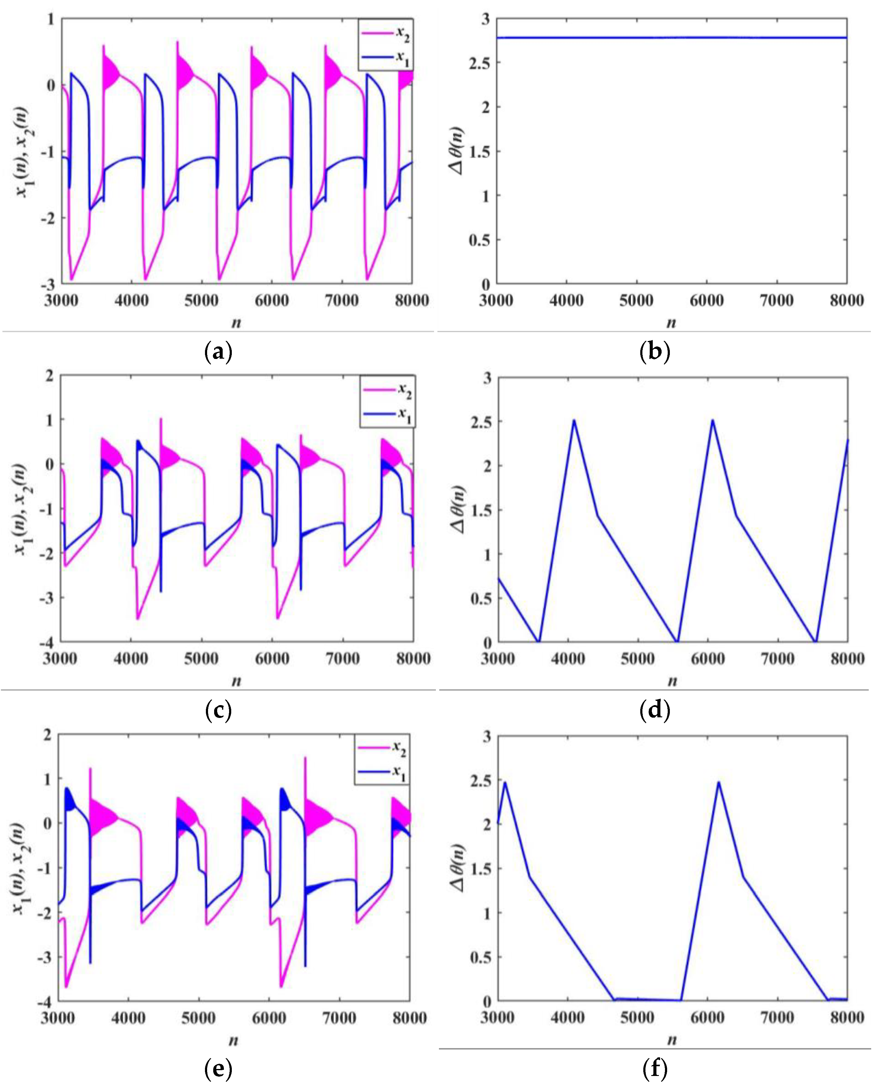
When α1 = 2 and α2 = 3, with the coupling strength k increasing from 0.1 to 0.5, the phenomenon of synchronization transition occurs, which is different from all the previous synchronization transitions. Figure 17a,c,e,g show firing patterns of two neurons and Figure 17b,d,f,h present phase difference between two neurons at k = 0.1, 0.25, 0.3, and 0.5 respectively. According to the time sequences shown in Figure 17a, it can be realized that the two neurons exhibit anti-phase synchronization at k = 0.1, and the firing patterns of the two Rulkov neurons are period-1 bursting firing and triangular bursting firing, respectively. The phase difference is maintained at a constant value in Figure 17b, which reflects the anti-phase synchronization behavior. When the coupling strength increases to 0.25, the firing patterns of the Rulkov neurons are mixed firing patterns, as presented in Figure 17c. As shown in Figure 17d, the phase difference is similar to a period function and fluctuates within the interval of [0, 3], which indicates that the Rulkov neurons are partially synchronized. Comparing Figure 17f with Figure 17d, it is obvious that the overall trend of the phase difference is similar, but it has a short stay at [4800, 5600]. When k = 0.5, the firing patterns of the two Rulkov neurons are triangular bursting firing, as presented in Figure 17g. Furthermore, it can be observed from Figure 17h that the phase difference between the two neurons remains constant, demonstrating the phenomenon of synchronization. Through the whole process, it is found that the firing patterns of the two Rulkov neurons change.
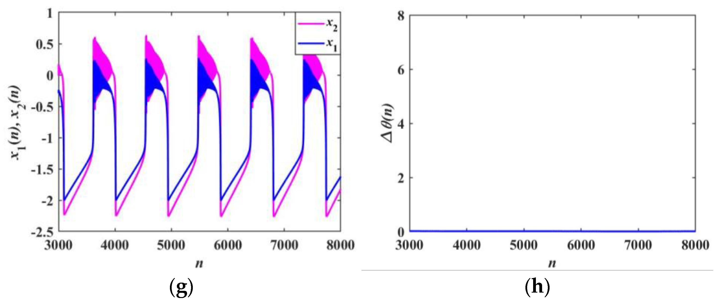
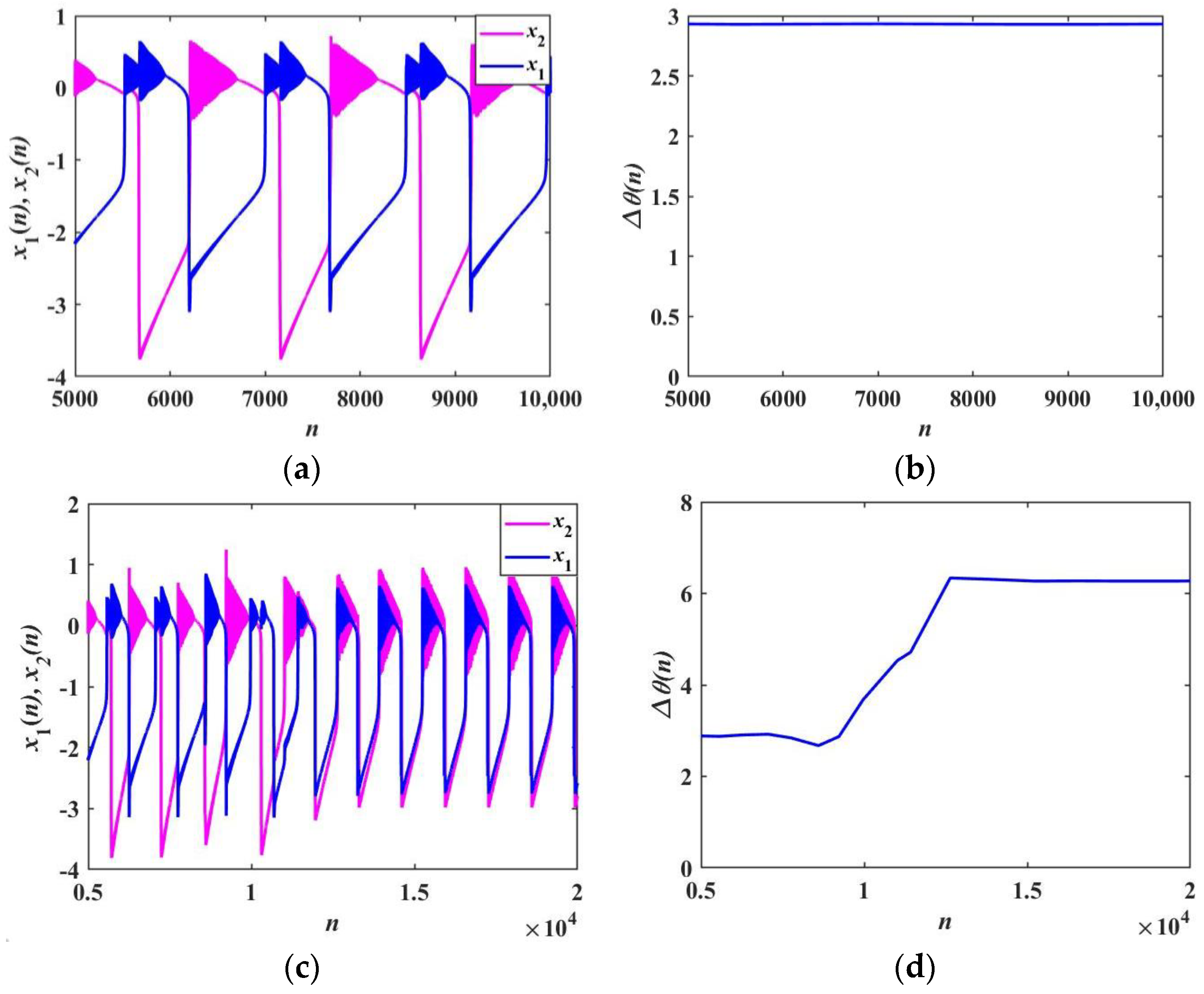
In addition, with α1 = 3 and α2 = 3.5, the synchronization transition behavior is depicted in Figure 18. When k increases from 0.1 to 0.15, the transition from anti-phase synchronization to in-phase synchronization takes place. Figure 18a,c,e show firing patterns of two neurons and Figure 18b,d,f present phase difference between two neurons with k = 0.1, 0.108, and 0.15 respectively. When the coupled strength k = 0.1, the two Rulkov neurons exhibit anti-phase synchronization with different triangular bursting firing patterns, as presented in Figure 18a,b. Figure 18c presents the intermediate transition process. Under different iteration times, the neurons present different synchronization behaviors. It can also be characterized by the phase difference shown in Figure 18d. When the coupled strength k = 0.15, the two neurons are exactly synchronized, as shown in Figure 18e,f. In the whole process, it is clear that the two Rulkov neurons do not produce new firing patterns as the coupling strength increases.
6. Conclusions
In this paper, a simple neural network was proposed, in which an LADM was used to mimic the synapse connecting two Rulkov neurons. Because of its bistable, nonlinear, and biomimetic characteristics, the LADM enriched the dynamic behaviors of the neural network. Through the numerical simulation of the IORNN and FORNN models, the transition of different firing patterns was explored. Furthermore, in the IORNN model, several novel firing patterns, including a bursting firing pattern with new topologies as well as mixed firing behaviors, were discovered. The firing behaviors of the neural network had high sensitivity to initial values, resulting in the coexisting behaviors of periodic and transient chaotic firing patterns, as well as period-1 bursting firing and triangular bursting firing patterns. In addition, the phase synchronization and synchronization transition were discussed in detail. When the neurons were weakly coupled, they were anti-phase synchronized. However, they were in-phase synchronized as the coupling strength increased. It is worth noting that we observed the anti-phase synchronization of coupled homogeneous neurons with different firing patterns, which is instructive for the analysis and understanding of neuronal activity in the different functional areas of the brain and the pathological research of some mental diseases. Our next work should be to analyze the mechanism of the dynamic behavior shown in this paper and to conduct more research on fractional-order neural network models.
Author Contributions
Conceptualization, M.M. and Y.L.; methodology, M.M. and Y.L.; validation, Y.L.; formal analysis, Z.L.; investigation, Y.L.; resources, M.M. and Z.L.; data curation, Z.L.; writing—original draft preparation, Y.L., M.M. and Y.S.; writing—review and editing, M.M. and Y.L.; visualization, C.W. and Y.S.; supervision, M.M. and Z.L.; project administration, Z.L.; funding acquisition, M.M., Z.L. and C.W. All authors have read and agreed to the published version of the manuscript.
Funding
This work was supported by the Natural Science Foundation of Hunan Province under Grant No. 2022JJ30572 and No. 2022JJ30160 and No. 2021JJ30671 and the Scientific Research Program through the Hunan Provincial Education Department under Grant No. 20C1772 and the National Natural Science Foundations of China under Grant No. 62171401.
Data Availability Statement
The datasets generated during and/or analyzed during the current study are available from the corresponding author upon reasonable request.
Conflicts of Interest
The authors declare no conflict of interest.
References
- Gomez-Gardenes, J.; Zamora-Lopez, G.; Moreno, Y.; Arenas, A. From Modular to Centralized Organization of Synchronization in Functional Areas of the Cat Cerebral Cortex. PLoS ONE 2010, 5, e12313. [Google Scholar] [CrossRef] [Green Version]
- Baker, S.N.; Spinks, R.; Jackson, A.; Lemon, R.N. Synchronization in monkey motor cortex during a precision grip task. I. Task-dependent modulation in single-unit synchrony. J. Neurophysiol. 2001, 85, 869–885. [Google Scholar] [CrossRef] [PubMed] [Green Version]
- Melloni, L.; Molina, C.; Pena, M.; Torres, D.; Singer, W.; Rodriguez, E. Synchronization of neural activity across cortical areas correlates with conscious perception. J. Neurosci. Off. J. Soc. Neurosci. 2007, 27, 2858–2865. [Google Scholar] [CrossRef] [PubMed] [Green Version]
- Mitchell, D.G.; Greening, S.G. Conscious perception of emotional stimuli: Brain mechanisms. Neuroscientist 2012, 18, 386–398. [Google Scholar] [CrossRef] [PubMed]
- Jiruska, P.; Csicsvari, J.; Powell, A.D.; Fox, J.E.; Chang, W.-C.; Vreugdenhil, M.; Li, X.; Palus, M.; Bujan, A.F.; Dearden, R.W.; et al. High-Frequency Network Activity, Global Increase in Neuronal Activity, and Synchrony Expansion Precede Epileptic Seizures In Vitro. J. Neurosci. 2010, 30, 5690–5701. [Google Scholar] [CrossRef] [Green Version]
- Stamoulis, C.; Gruber, L.J.; Chang, B.S. Network dynamics of the epileptic brain at rest. In Proceedings of the 2010 Annual International Conference of the IEEE Engineering in Medicine and Biology, Buenos Aires, Argentina, 31 August–4 September 2010; Volume 2010, pp. 150–153. [Google Scholar] [CrossRef] [Green Version]
- Li, Y.; Xiao, L.; Wei, Z.; Zhang, W. Zero-Hopf bifurcation analysis in an inertial two-neural system with delayed Crespi function. Eur. Phys. J. -Spec. Top. 2020, 229, 953–962. [Google Scholar] [CrossRef]
- Njitacke, Z.T.; Doubla, I.S.; Kengne, J.; Cheukem, A. Coexistence of firing patterns and its control in two neurons coupled through an asymmetric electrical synapse. Chaos 2020, 30, 023101. [Google Scholar] [CrossRef]
- Jin, J.; Zhu, J.; Zhao, L.; Chen, L.; Chen, L.; Gong, J. A Robust Predefined-Time Convergence Zeroing Neural Network for Dynamic Matrix Inversion. IEEE Trans. Cybern. 2022, 1–14. [Google Scholar] [CrossRef]
- Wan, Q.; Yan, Z.; Li, F.; Chen, S.; Liu, J. Complex dynamics in a Hopfield neural network under electromagnetic induction and electromagnetic radiation. Chaos 2022, 32, 073107. [Google Scholar] [CrossRef]
- Ma, J.; Tang, J. A review for dynamics in neuron and neuronal network. Nonlinear Dyn. 2017, 89, 1569–1578. [Google Scholar] [CrossRef]
- Yao, Z.; Sun, K.; He, S. Firing patterns in a fractional-order FithzHugh–Nagumo neuron model. Nonlinear Dyn. 2022, 110, 1807–1822. [Google Scholar] [CrossRef]
- Izhikevich, E.M. Simple model of spiking neurons. IEEE Trans. Neural Netw. 2003, 14, 1569–1572. [Google Scholar] [CrossRef] [Green Version]
- Rulkov, N.F.; Timofeev, I.; Bazhenov, M. Oscillations in large-scale cortical networks: Map-based model. J. Comput. Neurosci. 2004, 17, 203–223. [Google Scholar] [CrossRef]
- Tanaka, G.; Ibarz, B.; Sanjuan, M.A.F.; Aihara, K. Synchronization and propagation of bursts in networks of coupled map neurons. Chaos 2006, 16, 013113. [Google Scholar] [CrossRef] [PubMed]
- Cao, H.; Ibarz, B. Hybrid discrete-time neural networks. Philos. Trans. R. Soc. A-Math. Phys. Eng. Sci. 2010, 368, 5071–5086. [Google Scholar] [CrossRef]
- He, S.; Rajagopal, K.; Karthikeyan, A.; Srinivasan, A. A discrete Huber-Braun neuron model: From nodal properties to network performance. Cogn. Neurodynamics 2022, 1–10. [Google Scholar] [CrossRef]
- Lu, Y.; Wang, C.; Deng, Q. Rulkov neural network coupled with discrete memristors. Netw.-Comput. Neural Syst. 2022, 33, 214–232. [Google Scholar] [CrossRef] [PubMed]
- Wang, C.; Cao, H. Stability and chaos of Rulkov map-based neuron network with electrical synapse. Commun. Nonlinear Sci. Numer. Simul. 2015, 20, 536–545. [Google Scholar] [CrossRef]
- Hu, D.; Cao, H. Stability and synchronization of coupled Rulkov map-based neurons with chemical synapses. Commun. Nonlinear Sci. Numer. Simul. 2016, 35, 105–122. [Google Scholar] [CrossRef]
- Sun, H.; Cao, H. Complete synchronization of coupled Rulkov neuron networks. Nonlinear Dyn. 2016, 84, 2423–2434. [Google Scholar] [CrossRef]
- Sun, H.; Cao, H. Synchronization of two identical and non-identical Rulkov models. Commun. Nonlinear Sci. Numer. Simul. 2016, 40, 15–27. [Google Scholar] [CrossRef]
- Ge, P.; Cao, H. Synchronization of Rulkov neuron networks coupled by excitatory and inhibitory chemical synapses. Chaos 2019, 29, 023129. [Google Scholar] [CrossRef] [PubMed]
- Ferrari, F.A.S.; Viana, R.L.; Reis, A.S.; Iarosz, K.C.; Caldas, I.L.; Batista, A.M. A network of networks model to study phase synchronization using structural connection matrix of human brain. Phys. A-Stat. Mech. Its Appl. 2018, 496, 162–170. [Google Scholar] [CrossRef]
- Rakshit, S.; Ray, A.; Bera, B.K.; Ghosh, D. Synchronization and firing patterns of coupled Rulkov neuronal map. Nonlinear Dyn. 2018, 94, 785–805. [Google Scholar] [CrossRef]
- Chua, L. Memristor-the missing circuit element. IEEE Trans. Circuit Theory 1971, 18, 507–519. [Google Scholar] [CrossRef]
- Strukov, D.B.; Snider, G.S.; Stewart, D.R.; Williams, R.S. The missing memristor found. Nature 2008, 453, 80–83. [Google Scholar] [CrossRef]
- Wan, Q.; Yan, Z.; Li, F.; Liu, J.; Chen, S. Multistable dynamics in a Hopfield neural network under electromagnetic radiation and dual bias currents. Nonlinear Dyn. 2022, 109, 2085–2101. [Google Scholar] [CrossRef]
- Xu, Q.; Ju, Z.; Ding, S.; Feng, C.; Chen, M.; Bao, B. Electromagnetic induction effects on electrical activity within a memristive Wilson neuron model. Cogn. Neurodynamics 2022, 16, 1221–1231. [Google Scholar] [CrossRef] [PubMed]
- Lin, H.; Wang, C.; Cui, L.; Sun, Y.; Xu, C.; Yu, F. Brain-Like Initial-Boosted Hyperchaos and Application in Biomedical Image Encryption. IEEE Trans. Ind. Inform. 2022, 18, 8839–8850. [Google Scholar] [CrossRef]
- Wen, Z.; Wang, C.; Deng, Q.; Lin, H. Regulating memristive neuronal dynamical properties via excitatory or inhibitory magnetic field coupling. Nonlinear Dyn. 2022, 110, 3823–3835. [Google Scholar] [CrossRef]
- Yu, F.; Shen, H.; Yu, Q.; Kong, X.; Sharma, P.K.; Cai, S. Privacy Protection of Medical Data Based on Multiscroll Memristive Hopfield Neural Network. IEEE Trans. Netw. Sci. Eng. 2022, 1–14. [Google Scholar] [CrossRef]
- Ma, T.; Mou, J.; Yan, H.; Cao, Y. A new class of Hopfield neural network with double memristive synapses and its DSP implementation. Eur. Phys. J. Plus 2022, 137, 1135. [Google Scholar] [CrossRef]
- Chen, C.; Min, F.; Zhang, Y.; Bao, B. Memristive electromagnetic induction effects on Hopfield neural network. Nonlinear Dyn. 2021, 106, 2559–2576. [Google Scholar] [CrossRef]
- Du, S.; Deng, Q.; Hong, Q.; Li, J.; Liu, H.; Wang, C. A memristor-based circuit design and implementation for blocking on Pavlov associative memory. Neural Comput. Appl. 2022, 34, 14745–14761. [Google Scholar] [CrossRef]
- Yu, F.; Kong, X.; Mokbel, A.A.M.; Yao, W.; Cai, S. Complex Dynamics, Hardware Implementation and Image Encryption Application of Multiscroll Memeristive Hopfield Neural Network With a Novel Local Active Memeristor. IEEE Trans. Circuits Syst. II Express Briefs 2022, 70, 326–330. [Google Scholar] [CrossRef]
- Li, Z.; Yi, Z. A memristor-based associative memory circuit considering synaptic crosstalk. Electron. Lett. 2022, 58, 539–541. [Google Scholar] [CrossRef]
- Liang, Y.; Zhu, Q.; Wang, G.; Nath, S.K.; Iu, H.H.-C.; Nandi, S.K.; Elliman, R.G. Universal Dynamics Analysis of Locally-Active Memristors and Its Applications. IEEE Trans. Circuits Syst. I Regul. Pap. 2021, 69, 1278–1290. [Google Scholar] [CrossRef]
- Zhou, L.; You, Z.; Liang, X.; Li, X. A Memristor-Based Colpitts Oscillator Circuit. Mathematics 2022, 10, 4820. [Google Scholar] [CrossRef]
- Ding, D.; Xiao, H.; Yang, Z.; Luo, H.; Hu, Y.; Liu, Y.; Wang, M. Fractional-Order Heterogeneous Neuron Network With Hr Neuron and Fhn Neuron Based on Coupled Locally-Active Memristors: Super Coexisting Firing Behaviors, Bursting Behaviors and its Application. Bursting Behav. Its Appl. 2022. [Google Scholar] [CrossRef]
- Bao, B.; Yang, Q.; Zhu, D.; Zhang, Y.; Xu, Q.; Chen, M. Initial-induced coexisting and synchronous firing activities in memristor synapse-coupled Morris-Lecar bi-neuron network. Nonlinear Dyn. 2020, 99, 2339–2354. [Google Scholar] [CrossRef]
- Li, Z.; Zhou, H.; Wang, M.; Ma, M. Coexisting firing patterns and phase synchronization in locally active memristor coupled neurons with HR and FN models. Nonlinear Dyn. 2021, 104, 1455–1473. [Google Scholar] [CrossRef]
- Lin, H.; Wang, C.; Xu, C.; Zhang, X.; Iu, H.H. A memristive synapse control method to generate diversified multi-structure chaotic attractors. IEEE Trans. Comput. -Aided Des. Integr. Circuits Syst. 2022. [Google Scholar] [CrossRef]
- Shen, H.; Yu, F.; Wang, C.; Sun, J.; Cai, S. Firing mechanism based on single memristive neuron and double memristive coupled neurons. Nonlinear Dyn. 2022, 110, 3807–3822. [Google Scholar] [CrossRef]
- Zhang, J.; Liao, X. Synchronization and chaos in coupled memristor-based FitzHugh-Nagumo circuits with memristor synapse. AEU-Int. J. Electron. Commun. 2017, 75, 82–90. [Google Scholar] [CrossRef]
- Bao, H.; Zhang, Y.; Liu, W.; Bao, B. Memristor synapse-coupled memristive neuron network: Synchronization transition and occurrence of chimera. Nonlinear Dyn. 2020, 100, 937–950. [Google Scholar] [CrossRef]
- Wang, Y.; Min, F.; Cheng, Y.; Dou, Y. Dynamical analysis in dual-memristor-based FitzHugh-Nagumo circuit and its coupling finite-time synchronization. Eur. Phys. J. -Spec. Top. 2021, 230, 1751–1762. [Google Scholar] [CrossRef]
- Li, D.; Zhou, C. Organization of anti-phase synchronization pattern in neural networks: What are the key factors? Front. Syst. Neurosci. 2011, 5, 100. [Google Scholar] [CrossRef] [PubMed] [Green Version]
- Huang, L.; Liu, J.; Xiang, J.; Zhang, Z. Design and analysis of a three-dimensional discrete memristive chaotic map with infinitely wide parameter range. Phys. Scr. 2022, 97, 065210. [Google Scholar] [CrossRef]
- Lai, Q.; Lai, C. Design and Implementation of a New Hyperchaotic Memristive Map. IEEE Trans. Circuits Syst. II-Express Briefs 2022, 69, 2331–2335. [Google Scholar] [CrossRef]
- Yuan, F.; Xing, G.; Deng, Y. Flexible cascade and parallel operations of discrete memristor. Chaos Solitons Fractals 2023, 166, 112888. [Google Scholar] [CrossRef]
- Li, H.; Li, C.; Du, J. Discretized locally active memristor and application in logarithmic map. Nonlinear Dyn. 2022, 1–21. [Google Scholar] [CrossRef]
- Liang, Z.; He, S.; Wang, H.; Sun, K. A novel discrete memristive chaotic map. Eur. Phys. J. Plus 2022, 137, 309. [Google Scholar] [CrossRef]
- Ma, M.; Yang, Y.; Qiu, Z.; Peng, Y.; Sun, Y.; Li, Z.; Wang, M. A locally active discrete memristor model and its application in a hyperchaotic map. Nonlinear Dyn. 2022, 107, 2935–2949. [Google Scholar] [CrossRef]
- Wang, M.; An, M.; Zhang, X.; Iu, H.H.-C. Two-variable boosting bifurcation in a hyperchaotic map and its hardware implementation. Nonlinear Dyn. 2022, 111, 1871–1889. [Google Scholar] [CrossRef]
- Peng, Y.; He, S.; Sun, K. Parameter identification for discrete memristive chaotic map using adaptive differential evolution algorithm. Nonlinear Dyn. 2022, 107, 1263–1275. [Google Scholar] [CrossRef]
- He, S.; Zhan, D.; Wang, H.; Sun, K.; Peng, Y. Discrete Memristor and Discrete Memristive Systems. Entropy 2022, 24, 786. [Google Scholar] [CrossRef] [PubMed]
- Lai, Q.; Lai, C.; Zhang, H.; Li, C. Hidden coexisting hyperchaos of new memristive neuron model and its application in image encryption. Chaos Solitons Fractals 2022, 158, 112017. [Google Scholar] [CrossRef]
- Bao, H.; Hua, Z.; Liu, W.; Bao, B. Discrete memristive neuron model and its interspike interval-encoded application in image encryption. Sci. China-Technol. Sci. 2021, 64, 2281–2291. [Google Scholar] [CrossRef]
- Ma, M.; Xiong, K.; Li, Z.; Sun, Y. Dynamic Behavior Analysis and Synchronization of Memristor-Coupled Heterogeneous Discrete Neural Networks. Mathematics 2023, 11, 375. [Google Scholar] [CrossRef]
- Lu, Y.-M.; Wang, C.-H.; Deng, Q.-L.; Xu, C. The dynamics of a memristor-based Rulkov neuron with fractional-order difference. Chin. Phys. B 2022, 31, 060502. [Google Scholar] [CrossRef]
- Xu, Q.; Liu, T.; Feng, C.-T.; Bao, H.; Wu, H.-G.; Bao, B.-C. Continuous non-autonomous memristive Rulkov model with extreme multistability. Chin. Phys. B 2021, 30, 128702. [Google Scholar] [CrossRef]
- Li, C.; Yang, Y.; Yang, X.; Lu, Y. Application of discrete memristors in logistic map and Hindmarsh-Rose neuron. Eur. Phys. J. -Spec. Top. 2022, 231, 3209–3224. [Google Scholar] [CrossRef]
- Adhikari, S.P.; Sah, M.P.; Kim, H.; Chua, L.O. Three Fingerprints of Memristor. IEEE Trans. Circuits Syst. I-Regul. Pap. 2013, 60, 3008–3021. [Google Scholar] [CrossRef]
- Lin, H.; Wang, C.; Hong, Q.; Sun, Y. A Multi-Stable Memristor and its Application in a Neural Network. IEEE Trans. Circuits Syst. II-Express Briefs 2020, 67, 3472–3476. [Google Scholar] [CrossRef]
- Chua, L. Everything You Wish to Know About Memristors But Are Afraid to Ask. Radioengineering 2015, 24, 319–368. [Google Scholar] [CrossRef]
- Chua, L.O. Local activity is the origin of complexity. Int. J. Bifurc. Chaos 2005, 15, 3435–3456. [Google Scholar] [CrossRef] [Green Version]
- Rulkov, N.F. Regularization of synchronized chaotic bursts. Phys. Rev. Lett. 2001, 86, 183. [Google Scholar] [CrossRef] [Green Version]
- Wu, A.; Zeng, Z. Global Mittag-Leffler Stabilization of Fractional-Order Memristive Neural Networks. IEEE Trans. Neural Netw. Learn. Syst. 2017, 28, 206–217. [Google Scholar] [CrossRef]
- Huang, L.-L.; Park, J.H.; Wu, G.-C.; Mo, Z.-W. Variable-order fractional discrete-time recurrent neural networks. J. Comput. Appl. Math. 2020, 370, 112633. [Google Scholar] [CrossRef]
- He, S.; Sun, K.; Wang, H. Complexity Analysis and DSP Implementation of the Fractional-Order Lorenz Hyperchaotic System. Entropy 2015, 17, 8299–8311. [Google Scholar] [CrossRef]
Figure 1.
Pinched hysteresis loops of the LADM model with ϕ(0) = 0: (a) ω = 0.1 Hz; (b) A = 1.5 V.

Figure 2.
Pinched hysteresis loops of the LADM model with ϕ(0) = 0 and ϕ(0) = 2, respectively.

Figure 3.
Power-off plot (POP) with three equilibrium points.

Figure 4.
DC V–I diagram of the bistable LADM.

Figure 5.
SE complexity with variable paraments α and k: (a) IORNN; (b) FORNN with q = 0.6.

Figure 6.
Transition of firing patterns of the FORNN with q = 0.6 and α = 3: (a) k = 0.1; (b) k = 0.8; (c) k = 0.9.
Figure 6.
Transition of firing patterns of the FORNN with q = 0.6 and α = 3: (a) k = 0.1; (b) k = 0.8; (c) k = 0.9.

Figure 7.
Transition of firing patterns of the FORNN with q = 0.95 and α = 3: (a) k = 0.1; (b) k = 0.8; (c) k = 0.9.
Figure 7.
Transition of firing patterns of the FORNN with q = 0.95 and α = 3: (a) k = 0.1; (b) k = 0.8; (c) k = 0.9.

Figure 8.
Transition of firing patterns of the IORNN with α = 3: (a) k = 0.1; (b) k = 0.8; (c) k = 0.9.
Figure 8.
Transition of firing patterns of the IORNN with α = 3: (a) k = 0.1; (b) k = 0.8; (c) k = 0.9.

Figure 9.
Transition of firing patterns of the FORNN with q = 0.6 and α1 = 3, α2 = 4: (a) k = 0; (b) k = 0. 01; (c) k = 0.8.
Figure 9.
Transition of firing patterns of the FORNN with q = 0.6 and α1 = 3, α2 = 4: (a) k = 0; (b) k = 0. 01; (c) k = 0.8.

Figure 10.
Transition of firing patterns of the FORNN with q = 0.95 and α1 = 3, α2 = 4: (a) k = 0; (b) k = 0. 01; (c) k = 0.8.
Figure 10.
Transition of firing patterns of the FORNN with q = 0.95 and α1 = 3, α2 = 4: (a) k = 0; (b) k = 0. 01; (c) k = 0.8.

Figure 11.
Transition of firing patterns of the IORNN with α1 = 3, α2 = 4 (a) k = 0; (b) k = 0.01; (c) k = 0.8.
Figure 11.
Transition of firing patterns of the IORNN with α1 = 3, α2 = 4 (a) k = 0; (b) k = 0.01; (c) k = 0.8.

Figure 12.
Firing patterns with α1 = 2.5 and α2 = 2: (a,c) the time sequences of x1 with k = 0.1 and 0.2, respectively; (b,d) the time sequences of x2 with k = 0.1 and 0.2, respectively.
Figure 12.
Firing patterns with α1 = 2.5 and α2 = 2: (a,c) the time sequences of x1 with k = 0.1 and 0.2, respectively; (b,d) the time sequences of x2 with k = 0.1 and 0.2, respectively.


Figure 13.
Firing patterns with α1 = 3 and α2 = 2: (a–c) the time sequences of x1 with k = 0.2, 0.3, and 0.4; (d–f) the time sequences of x2 with k = 0.2, 0.3, and 0.4.
Figure 13.
Firing patterns with α1 = 3 and α2 = 2: (a–c) the time sequences of x1 with k = 0.2, 0.3, and 0.4; (d–f) the time sequences of x2 with k = 0.2, 0.3, and 0.4.

Figure 14.
Time series and phase diagrams for different iteration times: (a) time series of x1 with n = [3000, 10,000]; (b) attractor with n = [3000, 10,000]; (c) time series of x1 with n = [10,000, 18,000]; (d) attractor with n = [10,000, 18,000].
Figure 14.
Time series and phase diagrams for different iteration times: (a) time series of x1 with n = [3000, 10,000]; (b) attractor with n = [3000, 10,000]; (c) time series of x1 with n = [10,000, 18,000]; (d) attractor with n = [10,000, 18,000].

Figure 15.
Coexisting firing pattern: (a) periodic firing pattern with initial values (−1.1, −3, −1, −3, 0.8); (b) transient chaotic firing pattern with initial values (−1, 0.5, −1, 0, 0).
Figure 15.
Coexisting firing pattern: (a) periodic firing pattern with initial values (−1.1, −3, −1, −3, 0.8); (b) transient chaotic firing pattern with initial values (−1, 0.5, −1, 0, 0).

Figure 16.
Coexisting firing pattern with α = 2.5: (a) time series with two different initial values of (1, 0.5, 1, 0.51, 0.3) and (1, 0.5, 1, 0, 1); (b) coexisting attractors with two different initial values of (1, 0.5, 1, 0.51, 0.3) and (1, 0.5, 1, 0, 1).
Figure 16.
Coexisting firing pattern with α = 2.5: (a) time series with two different initial values of (1, 0.5, 1, 0.51, 0.3) and (1, 0.5, 1, 0, 1); (b) coexisting attractors with two different initial values of (1, 0.5, 1, 0.51, 0.3) and (1, 0.5, 1, 0, 1).

Figure 17.
Firing patterns and phase difference with α1 = 2 and α2 = 3: (a,b) k = 0.1; (c,d) k = 0.25; (e,f) k = 0.3; (g,h) k = 0.5.
Figure 17.
Firing patterns and phase difference with α1 = 2 and α2 = 3: (a,b) k = 0.1; (c,d) k = 0.25; (e,f) k = 0.3; (g,h) k = 0.5.


Figure 18.
Firing patterns and phase difference with α1 = 3 and α2 = 3.5: (a,b) k = 0.1; (c,d) k = 0.108; (e,f) k = 0.15.
Figure 18.
Firing patterns and phase difference with α1 = 3 and α2 = 3.5: (a,b) k = 0.1; (c,d) k = 0.108; (e,f) k = 0.15.


Disclaimer/Publisher’s Note: The statements, opinions and data contained in all publications are solely those of the individual author(s) and contributor(s) and not of MDPI and/or the editor(s). MDPI and/or the editor(s) disclaim responsibility for any injury to people or property resulting from any ideas, methods, instructions or products referred to in the content. |
© 2023 by the authors. Licensee MDPI, Basel, Switzerland. This article is an open access article distributed under the terms and conditions of the Creative Commons Attribution (CC BY) license (https://creativecommons.org/licenses/by/4.0/).
Share and Cite
MDPI and ACS Style
Ma, M.; Lu, Y.; Li, Z.; Sun, Y.; Wang, C. Multistability and Phase Synchronization of Rulkov Neurons Coupled with a Locally Active Discrete Memristor. Fractal Fract. 2023, 7, 82. https://doi.org/10.3390/fractalfract7010082
AMA Style
Ma M, Lu Y, Li Z, Sun Y, Wang C. Multistability and Phase Synchronization of Rulkov Neurons Coupled with a Locally Active Discrete Memristor. Fractal and Fractional. 2023; 7(1):82. https://doi.org/10.3390/fractalfract7010082
Chicago/Turabian StyleMa, Minglin, Yaping Lu, Zhijun Li, Yichuang Sun, and Chunhua Wang. 2023. "Multistability and Phase Synchronization of Rulkov Neurons Coupled with a Locally Active Discrete Memristor" Fractal and Fractional 7, no. 1: 82. https://doi.org/10.3390/fractalfract7010082